A spatio-temporal model for extreme precipitation simulated by a climate model.

Transcription

1 A spatio-temporal model for extreme precipitation simulated by a climate model. Jonathan Jalbert Joint work with Anne-Catherine Favre, Claude Bélisle and Jean-François Angers STATMOS Workshop: Climate and Weather Extremes October 25 th, 2016 Pennsylvania State University, USA.

2 Introduction Jalbert et al. A spatio-temporal model for extreme precipitation simulated by a climate model 2016/10/25 2 / 30

3 Goal With climate, in situ experimentations are impossible. Climate models are therefore the only tools for providing quantitative predictions of the coming climate. The goal of the talk is to present a spatio-temporal statistical model especially suited for extreme precipitation simulated by a climate model. More specifically, the statistical model takes into account non-stationarity in transient time series; large spatial simulation domain; spatial dependence among grid points. Jalbert et al. A spatio-temporal model for extreme precipitation simulated by a climate model 2016/10/25 3 / 30

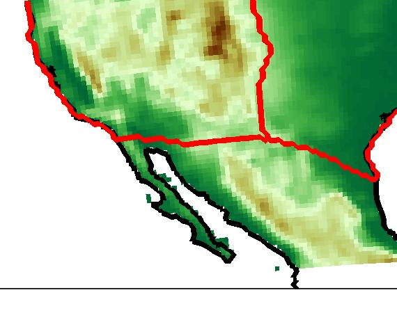
4 Data The dataset consists in the daily precipitation outputs from a run of the Canadian Regional Climate Model (CRCM). The data were simulated and provided by 12,570 land grid points; Daily precipitation series for the period [1961, 2100] at every grid point. Let Y ikl be the precipitation depth (mm) of day l of year k at grid point i, where 1 i 12, 570; 1 k 140; 1 l 365. Simulation domain Jalbert et al. A spatio-temporal model for extreme precipitation simulated by a climate model 2016/10/25 4 / 30

5 Non-Stationarity Jalbert et al. A spatio-temporal model for extreme precipitation simulated by a climate model 2016/10/25 5 / 30

6 Non-stationarity in the maxima series Let M ik be the annual maximum of year k at grid point i: M ik = max 1 l 365 Y ikl. Let M i be the annual maxima series at grid point i: M i = (M ik : 1 k 140). For 2/3 of the grid points, the series of maxima M i exhibits temporal non-stationarity (the grid points in red in the following figure). Jalbert et al. A spatio-temporal model for extreme precipitation simulated by a climate model 2016/10/25 6 / 30

7 Non-stationarity in the maxima series Let M ik be the annual maximum of year k at grid point i: M ik = max 1 l 365 Y ikl. Let M i be the annual maxima series at grid point i: M i = (M ik : 1 k 140). For 2/3 of the grid points, the series of maxima M i exhibits temporal non-stationarity (the grid points in red in the following figure). Pointwise Mann-Kendall stationarity test (α = 5%) Jalbert et al. A spatio-temporal model for extreme precipitation simulated by a climate model 2016/10/25 6 / 30

8 Maxima series - Montreal Maximum (mm) Year Jalbert et al. A spatio-temporal model for extreme precipitation simulated by a climate model 2016/10/25 7 / 30

9 Introduction Non-Stationarity Spatial modeling Results Conclusion Daily series - Montreal 100 Precipitation (mm) Year Jalbert et al. A spatio-temporal model for extreme precipitation simulated by a climate model 2016/10/25 8 / 30

10 Introduction Non-Stationarity Spatial modeling Results Conclusion Exceedances - Montreal 100 Precipitation (mm) Year Jalbert et al. A spatio-temporal model for extreme precipitation simulated by a climate model 2016/10/25 9 / 30

11 Preprocessing approach Suppose that there exist sequences of constants ν ik and τ ik such that ( M ik = M ) ik ν ik : 1 k 140 ; (1) τ ik can be assumed identically distributed along index k for each grid point i. Therefore, the distribution of a given transformed maximum can be approximated by M ik L GEV (µ i, σ i, ξ i ). (2) The trend in the tail should be isolated from the trend in the bulk of the distribution. Jalbert et al. A spatio-temporal model for extreme precipitation simulated by a climate model 2016/10/25 10 / 30

12 Preprocessing approach Suppose that there exist sequences of constants ν ik and τ ik such that ( M ik = M ) ik ν ik : 1 k 140 ; (1) τ ik can be assumed identically distributed along index k for each grid point i. Therefore, the distribution of a given transformed maximum can be approximated by M ik L GEV (µ i, σ i, ξ i ). (2) The trend in the tail should be isolated from the trend in the bulk of the distribution. Jalbert et al. A spatio-temporal model for extreme precipitation simulated by a climate model 2016/10/25 10 / 30

13 Introduction Non-Stationarity Spatial modeling Results Conclusion Preprocessing approach Let Zik be the vector of precipitation exceedences over the threshold ui of year k at grid point i: 100 and let Precipitation (mm) 80 Zik = (Yikl : Yikl > ui, 1 l 140) ; νik = E(Zik ) and τik2 = Var (Zik ) Year The threshold has to be chosen in order that the transformation: Mik0 = Mik νik ; τik (3) removes the trend in the maxima series Mi0. Its definition does not rely on asymptotic convergence requirements as in the Peaks-Over-Threshold model. Jalbert et al. A spatio-temporal model for extreme precipitation simulated by a climate model 2016/10/25 11 / 30

14 Introduction Non-Stationarity Spatial modeling Results Conclusion Preprocessing approach Let Zik be the vector of precipitation exceedences over the threshold ui of year k at grid point i: 100 and let Precipitation (mm) 80 Zik = (Yikl : Yikl > ui, 1 l 140) ; νik = E(Zik ) and τik2 = Var (Zik ) Year The threshold has to be chosen in order that the transformation: Mik0 = Mik νik ; τik (3) removes the trend in the maxima series Mi0. Its definition does not rely on asymptotic convergence requirements as in the Peaks-Over-Threshold model. Jalbert et al. A spatio-temporal model for extreme precipitation simulated by a climate model 2016/10/25 11 / 30

15 Preprocessed maxima series - Montreal Maximum (mm) p < Standardized Maximum Year Jalbert et al. A spatio-temporal model for extreme precipitation simulated by a climate model 2016/10/25 12 / 30

16 Preprocessed maxima series - Montreal Maximum (mm) Standardized Maximum Year Jalbert et al. A spatio-temporal model for extreme precipitation simulated by a climate model 2016/10/25 12 / 30

17 Preprocessed maxima series - Montreal 1 20 p =0.22 Maximum (mm) Standardized Maximum Year Jalbert et al. A spatio-temporal model for extreme precipitation simulated by a climate model 2016/10/25 12 / 30

18 Threshold choice We chose the 80th empirical quantiles at each grid point as the thresholds. Then, the stationarity hypothesis of the preprocessed maxima series was rejected for only 1.5% of the grid points (the grid points in red in the following figure). Pointwise Mann-Kendall stationarity test (α = 5%) for the preprocessed maxima series Jalbert et al. A spatio-temporal model for extreme precipitation simulated by a climate model 2016/10/25 13 / 30

19 Preprocessing approach Benefits of the proposed preprocessing approach are: if there exist constants a ik > 0 and b ik such that M ik b ik a ik L GEV (0, 1, ξi ); then there exists constants a ik > 0 and b ik such that M ik b ik a ik L GEV (0, 1, ξ i ). The model for the untransformed maxima is tractable: M ik L GEV (τik µ i + ν ik, τ ik σ i, ξ i ). (4) Jalbert et al. A spatio-temporal model for extreme precipitation simulated by a climate model 2016/10/25 14 / 30

20 Preprocessing approach Benefits of the proposed preprocessing approach are: if there exist constants a ik > 0 and b ik such that M ik b ik a ik L GEV (0, 1, ξi ); then there exists constants a ik > 0 and b ik such that M ik b ik a ik L GEV (0, 1, ξ i ). The model for the untransformed maxima is tractable: M ik L GEV (τik µ i + ν ik, τ ik σ i, ξ i ). (4) Jalbert et al. A spatio-temporal model for extreme precipitation simulated by a climate model 2016/10/25 14 / 30

21 Spatial modeling Jalbert et al. A spatio-temporal model for extreme precipitation simulated by a climate model 2016/10/25 15 / 30

22 Spatial dependence structure Following the idea of Cooley & Sain (2010) and Reich & Shaby (2012), the spatial dependence is taken into account by modeling spatial variation in the GEV parameters mainly for two reasons: such a latent variable approach is very flexible; the local properties of extremal distributions (such as return levels) are well reproduced (Davison et al., 2012; Sebille et al., 2016). However such an approach can neither model nor predict an event occurring simultaneously at several grid points. Jalbert et al. A spatio-temporal model for extreme precipitation simulated by a climate model 2016/10/25 16 / 30

23 Spatial latent model Local estimates of the GEV location parameter. Local parameter estimates could definitely benefit from neighboring site values. Jalbert et al. A spatio-temporal model for extreme precipitation simulated by a climate model 2016/10/25 17 / 30

24 Spatial latent model Local estimates of the GEV scale parameter. Local parameter estimates could definitely benefit from neighboring site values. Jalbert et al. A spatio-temporal model for extreme precipitation simulated by a climate model 2016/10/25 17 / 30

25 Spatial latent model Local estimates of the GEV shape parameter. Local parameter estimates could definitely benefit from neighboring site values. Jalbert et al. A spatio-temporal model for extreme precipitation simulated by a climate model 2016/10/25 17 / 30

26 Spatial latent model Because the random variables lie on a regular lattice, Gaussian Markov random fields are well appropriate. Such a field inherits the Markov property. For the GEV location parameter, we have: µ i f [µi µ i =µ i ](µ i ) = f [µi µ δi =µ δi ](µ i ); where δ i is the set of neighbors of grid point i. The precision matrix Q of the joint distribution of µ is sparse because of the important following simplification: µ i µ j µ i, j q ij = 0; (5) where q ij is the element (i, j) of the precision matrix Q. Jalbert et al. A spatio-temporal model for extreme precipitation simulated by a climate model 2016/10/25 18 / 30

27 Spatial latent model Because the random variables lie on a regular lattice, Gaussian Markov random fields are well appropriate. Such a field inherits the Markov property. For the GEV location parameter, we have: µ i f [µi µ i =µ i ](µ i ) = f [µi µ δi =µ δi ](µ i ); where δ i is the set of neighbors of grid point i. The precision matrix Q of the joint distribution of µ is sparse because of the important following simplification: µ i µ j µ i, j q ij = 0; (5) where q ij is the element (i, j) of the precision matrix Q. Jalbert et al. A spatio-temporal model for extreme precipitation simulated by a climate model 2016/10/25 18 / 30

28 Intrinsic Gaussian Markov random fields A Gaussian Markov Random field is a multivariate normal vector µ = (µ i, i = 1,..., n) where the precision matrix Q fulfills the following property: q ij = 0 if µ i µ j µ i, j. The marginal pairwise correlation that can be modeled by Gaussian Markov random fields is limited to 0.8 (Besag & Kooperberg, 1995). An option is to use intrinsic Gaussian Markov random fields, where the precision matrix is not of full rank. The rank deficiency controls the smoothness of the field. First-order igmrfs better capture small-scale variations whereas second-order igmrfs better model large-scale ones. Jalbert et al. A spatio-temporal model for extreme precipitation simulated by a climate model 2016/10/25 19 / 30

29 Intrinsic Gaussian Markov random fields The most popular igmrfs are defined with a scaled precision matrix: Q = κw ; where 0 < κ < is a precision parameter that controls the smoothness of the field and W is a structure matrix known from the grid. Let k be the rank deficiency of the precision matrix Q. The improper joint distribution is proportional to { f µ (µ) κ n k 2 exp κ } 2 µ W µ. Under the Bayesian paradigm, igmrfs generally yield proper posterior distributions when used as prior. Jalbert et al. A spatio-temporal model for extreme precipitation simulated by a climate model 2016/10/25 20 / 30

30 First-order intrinsic Gaussian Markov random fields Let n i = Card(δ i ), be the number of neighbors of grid point i. 1 1 f [µi µ δi =µ δi ](µ i ) = N µ i µ j, ; n i κn i j δ i µ i where κ > 0 is the precision parameter. This model approximates a two-dimensional Brownian motion. Jalbert et al. A spatio-temporal model for extreme precipitation simulated by a climate model 2016/10/25 21 / 30

31 First-order intrinsic Gaussian Markov random fields Let n i = Card(δ i ), be the number of neighbors of grid point i. 1 1 f [µi µ δi =µ δi ](µ i ) = N µ i µ j, ; n i κn i j δ i µ i where κ > 0 is the precision parameter. This model approximates a two-dimensional Brownian motion. Jalbert et al. A spatio-temporal model for extreme precipitation simulated by a climate model 2016/10/25 21 / 30

32 Second-order intrinsic Gaussian Markov random fields E(X i X i = x i ) = Prec(X i X i = x i ) = 20κ. This model is an approximation to the thin plate spline, the two-dimensional extension of cubic splines. µ i Jalbert et al. A spatio-temporal model for extreme precipitation simulated by a climate model 2016/10/25 22 / 30

33 Second-order intrinsic Gaussian Markov random fields E(X i X i = x i ) = Prec(X i X i = x i ) = 20κ. -1/20 This model is an approximation to the thin plate spline, the two-dimensional extension of cubic splines. -2/20 8/20-2/20-1/20 8/20 µ i 8/20-1/20-2/20 8/20-2/20-1/20 Jalbert et al. A spatio-temporal model for extreme precipitation simulated by a climate model 2016/10/25 22 / 30

34 Complete spatial model The model is therefore: f [M ik (µi,φi,ξi )] (m ik ) L GEV {m ik µ i, exp (φ i ), ξ i } ; f (µ,φ,ξ) (µ, φ, ξ) { (κ µ κ φ κ ξ ) n k 2 exp κ µ 2 µ W µ κ φ 2 φ W φ κ } ξ 2 ξ W ξ ; Three independent intrinsic Gaussian Markov random fields for the GEV parameter prior. Vague gamma hyperpriors for the precision parameters. Also, igmrfs are semi-informative: marginally non-informative, for example E(µ i ) is undefined and Var(µ i ) = ; spatially informative. Jalbert et al. A spatio-temporal model for extreme precipitation simulated by a climate model 2016/10/25 23 / 30

35 Complete spatial model The model is therefore: f [M ik (µi,φi,ξi )] (m ik ) L GEV {m ik µ i, exp (φ i ), ξ i } ; f (µ,φ,ξ) (µ, φ, ξ) { (κ µ κ φ κ ξ ) n k 2 exp κ µ 2 µ W µ κ φ 2 φ W φ κ } ξ 2 ξ W ξ ; Three independent intrinsic Gaussian Markov random fields for the GEV parameter prior. Vague gamma hyperpriors for the precision parameters. Also, igmrfs are semi-informative: marginally non-informative, for example E(µ i ) is undefined and Var(µ i ) = ; spatially informative. Jalbert et al. A spatio-temporal model for extreme precipitation simulated by a climate model 2016/10/25 23 / 30

36 Results Jalbert et al. A spatio-temporal model for extreme precipitation simulated by a climate model 2016/10/25 24 / 30

37 Homogeneous regions Jalbert et al. A spatio-temporal model for extreme precipitation simulated by a climate model 2016/10/25 25 / 30

38 Chosen model Spatial estimates of the GEV location parameter. According to the deviance information criterion, the model with the second-order igmrf prior is better. Jalbert et al. A spatio-temporal model for extreme precipitation simulated by a climate model 2016/10/25 26 / 30

39 Chosen model Spatial estimates of the GEV scale parameter. According to the deviance information criterion, the model with the second-order igmrf prior is better. Jalbert et al. A spatio-temporal model for extreme precipitation simulated by a climate model 2016/10/25 26 / 30

40 Chosen model Spatial estimates of the GEV shape parameter. According to the deviance information criterion, the model with the second-order igmrf prior is better. Jalbert et al. A spatio-temporal model for extreme precipitation simulated by a climate model 2016/10/25 26 / 30

41 Model fit κ ξ κ σ κ µ Iteration Jalbert et al. A spatio-temporal model for extreme precipitation simulated by a climate model 2016/10/25 27 / 30

42 Application - Projected return level Estimated quantiles (mm) Observed annual precipitation maxima [1943, 1994] at Montreal Trudeau airport year return level (mm) Projected 20-year return level at Montreal Trudeau airport Spatial model Marginal model Empirical quantiles (mm) year Jalbert et al. A spatio-temporal model for extreme precipitation simulated by a climate model 2016/10/25 28 / 30

43 Conclusion Jalbert et al. A spatio-temporal model for extreme precipitation simulated by a climate model 2016/10/25 29 / 30

44 Conclusion The statistical model developed was well suited for climate model outputs, specifically for: transient time series; data that lie on a regular grid but could also be adapted to irregular locations (Lindgren et al., 2011, Paciorek, 2013). The model s simplicity, intuitive interpretation and uncertainty description along with its fast adjustment make it very appealing. Nevertheless, the model could be enhanced by integrating several climate simulations for a better description of future climate uncertainty; We are also investigating the application of max-stable hierarchical models (Shaby & Reich, 2012). Jalbert et al. A spatio-temporal model for extreme precipitation simulated by a climate model 2016/10/25 30 / 30

45 Conclusion The statistical model developed was well suited for climate model outputs, specifically for: transient time series; data that lie on a regular grid but could also be adapted to irregular locations (Lindgren et al., 2011, Paciorek, 2013). The model s simplicity, intuitive interpretation and uncertainty description along with its fast adjustment make it very appealing. Nevertheless, the model could be enhanced by integrating several climate simulations for a better description of future climate uncertainty; We are also investigating the application of max-stable hierarchical models (Shaby & Reich, 2012). Jalbert et al. A spatio-temporal model for extreme precipitation simulated by a climate model 2016/10/25 30 / 30

46 Appendix Appendix Jalbert et al. A spatio-temporal model for extreme precipitation simulated by a climate model 2016/10/25 31 / 30

47 Appendix Gaussian Markov random fields For a stationary field in space, the conditional distributions have to take the following form: f [µi µ δi =µ δi ](µ i ) = N µ i η i + ρ (µ j η j ), ζ 2 ; (6) j δ i where 0 ρ 1 and ζ 2 > 0. It can be shown that marginal bivariate correlation coefficients between neighbors are necessarily less than 0.8: (Besag & Kooperberg, 1995) Cor(µ i, µ j ) 0.8, for j δ i. (7) The spatial correlation that can be modeled is therefore limited. Jalbert et al. A spatio-temporal model for extreme precipitation simulated by a climate model 2016/10/25 32 / 30

48 Appendix Model fit A chain of length 6000 was generated where the first 1000 iterations were discarded as the burn-in period. It took less than 40 minutes of computation time on a 2.53 GHz processor. algorithms for sparse matrix; parallel MCMC. Jalbert et al. A spatio-temporal model for extreme precipitation simulated by a climate model 2016/10/25 33 / 30

49 Appendix Modeling the dependence between the GEV paremeters We could consider a multivariate intrinsic Gaussian Markov random field as follows: f (µ,φ,ξ) (µ, φ, ξ) Γ ( exp µ, φ, ξ ) Γ µ φ, ξ Under a separability assumption, Benerjee et al. (2004) proposed to model the precision matrix Γ as follows: κ µ γ µφ γ µξ Γ = γ µφ κ φ γ φξ W, γ µξ γ φξ κ ξ To ensure parameter identifiability, Cooley & Sain (2010) and Economou et al. (2014) fixed the precision of the Gaussian Markov fields modeling the spatial dependence between each GEV parameters. Jalbert et al. A spatio-temporal model for extreme precipitation simulated by a climate model 2016/10/25 34 / 30

50 Appendix Application - Postprocessing Postprocessing of the annual maxima series at the grid point containing Montreal Trudeau airport Simulated Postprocessed Annual maxima (mm) Year Jalbert et al. A spatio-temporal model for extreme precipitation simulated by a climate model 2016/10/25 35 / 30