FINAL REPORT. Tessellation, Fairing, Shape Design, and Trimming Techniques for Subdivision Surface based Modeling

Transcription

1 FINAL REPORT Tessellation, Fairing, Shape Design, and Trimming Techniques for Subdivision Surface based Modeling (DMS ) PI: Fuhua (Frank) Cheng Department of Computer Science College of Engineering University of Kentucky Tel: (859) cheng/ 10/10/2008

2 Report Summary This final report summarizes the work we did for the grant DMI Subdivision surfaces are capable of modeling and representing complex shape of arbitrary topology. However, methods on how to build the control mesh of a complex surface have not been studied much. Currently, most meshes of complicated objects come from triangulation and simplification of raster scanned data points, like the Stanford 3D Scanning Repository. This approach is costly and leads to very dense meshes. In this project, we develop necessary mathematical theories and geometric algorithms to support subdivision surface based modeling. First, an explicit parametrization method is presented for exact evaluation of Catmull-Clark subdivision surfaces. Based on our parametrization techniques, four modeling techniques have been developed for constructing the control mesh of a given object with arbitrary topology. The first technique is adaptive tessellation. By performing recursive adaptive subdivision of an initial mesh, we can get the control mesh of a given object with the same geometric appearance and properties but with much less nodes in the control mesh of the object. This work needs the capability of estimating the subdivision depth of the given object within a given error tolerance before hand. The subdivision depth computation technique is presented in this report. The second technique is automatic fairing. The idea is to identify regions of an object with extra-ordinary curvature values and replace those regions with surfaces of smaller curvature values. A local parametrization based curvature computation technique for triangular meshes has been developed. The new technique allows curvature to be computed in any direction for any point of the given mesh and guarantees higher accuracy of the computed results because our technique is based on a precise representation of the object obtained by an interpolation process. Consequence, the new technique promises better fairing results. The third technique is interpolation based shape design. By sampling some representative points from a given object model, a control mesh can be constructed and its subdivision surface interpolates all the sampled representative points and meanwhile is very close to the

3 given data model. Interpolation is a simple way to build models, but the fairness of the interpolating surface is a big concern in previous methods. By using similarity based interpolation, we can obtain better modeling result with less undesired artifacts and undulations. The result can also be filtered by our automatic fairing process to ensure smoothness of the interpolating surface. The fourth technique is trimming, i.e., to construct the control mesh of the final object in a design process through Boolean operations such union, difference and/or intersection. Boolean operations are a natural way of constructing complex solid objects out of simpler primitives. Up to this point, accurate Boolean operations over subdivision surfaces are not available in the literature yet. We developed a robust and error controllable Boolean operation method which is based on voxelization of subdivision surfaces. Different from previous voxelization based Boolean operation methods, our method results in a continuous geometric representation, i.e., a polygonal mesh of the resulting Boolean operations, which can be regarded as a one-piece representation of the final object. Because the resulting polygonal mesh is very dense, error controllable simplification of the control meshes is needed. This can be achieved through our adaptive tessellation technique discussed above. The adaptive tessellation technique can significantly reduce the complexity of a polygonal mesh and meanwhile have accurate error estimation. A system that performs subdivision surface based modeling is implemented and quite a few examples have been tested. All the examples show that our modeling techniques can obtain very good subdivision based representation results. Even though in some cases our methods are based on Catmull-Clark subdivision scheme only, they can be adapted to other subdivision schemes easily with just minor modifications. Overall, we consider this grant a big success. In addition to reaching all our research goals, we have also produced a PhD (Dr. Shuhua Lai, graduated in August, 2006, currently an Assistant Professor at the Virginia State University), an MS (Mr. Gang Chen, graduated in December 2006, currently working in L.A., California), 17 journal papers and 3 conference

4 papers. Another MS (Mr. Conglin Huang) will be produced at the end of this year (2008) and another PhD (Mr. Fengtao Fan) will be be produced at the end of next year (2009). The remaining part of the report is arranged as follows. In Chapter 1, we present a parametrization technique for Catmull-Clark subdivision surfaces. Our tessellation techniques for subdivision surfaces are shown in Chapter 2. Our curvature computation method for automatic fairing is shown in Chapter 3. Our subdivision depth computation techniques and voxelization techniques are shown in Chapters 4 and 5, respectively. Our interpolation based shape design techniques are shown in Chapter 6. Our trimming techniques for subdivision surfaces and their applications are shown in Chapter 7. Finally in Chapter 8, we present the structure of a subdivision surface based modeling system.

5 Table of Contents 1 Subdivision Surface Parametrization and Evaluation Previous Work New Parametrization Technique Applications Fast, Exact and Explicit Rendering Generating Special Features Texture Mapping Surface Trimming Adaptive Rendering Interpolation Boolean Operations Tessellation of Subdivision Surfaces Previous Work New Technique Inscribed Approximation Adaptive Inscribed Approximation Crack Elimination Degree of Flatness Algorithms of Adaptive Tessellation Global Index ID Adaptive Marking Adaptive Rendering a Single Patch Implementation and Test Results Automatic Fairing : Curvature Computation Previous Work Main Idea Local Interpolation Local Blending Curvature Computation Test Results Subdivision Depth Estimation Subdivision Depth Computation for Extra-Ordinary Patches Distance Evaluation

6 4.1.2 Subdivision Depth Computation New Subdivision Depth Computation Technique for Extra-Ordinary Patches Matrix based Rate of Convergence Distance Evaluation Subdivision Depth Computation Examples Voxelization of Free-form Solids Previous Voxelization Techniques Voxelization based on Recursive Subdivision Separability, Accuracy and Minimality Volume Flooding with Dynamic Programming Seed Selection D Flooding using Dynamic Programming Applications Visualization of Complex Scenes Integral Properties Measurement Performing Boolean and CSG Operations Shape Design: Interpolation based Previous Work Similarity based Interpolation Mathematical Setup Interpolation Requirements Similarity Constraints Global Linear System Additional Interpolation Requirements Interpolation of Normal Vectors Handling Open Meshes Test Results Trimming of Subdivision Surfaces and Applications Related Work Performing Boolean Operations on Free-Form Solids Boolean Operations based on Recursive Subdivision & Voxelization Crack Prevention Local Voxelization Error Control Test Results Subdivision Surface based Modeling 78 Bibliography 78

7 Chapter 1 Subdivision Surface Parametrization and Evaluation In this chapter, a new parametrization technique and its applications for general Catmull- Clark subdivision surfaces [70] are presented. Our new technique [70] extends J. Stam s work [29] by redefining all the eigen basis functions in the parametric representation for general Catmull-Clark subdivision surfaces and giving each of them an explicit form. The entire eigen structure of the subdivision matrix and its inverse are computed exactly and explicitly with no need to precompute anything. Therefore, the new representation can be used not only for evaluation purpose, but for analysis purpose as well. The new approach is based on an Ω-partition [29] of the parameter space and a detoured subdivision path. This results in a block diagonal matrix with constant size diagonal blocks (7 7) for the corresponding subdivision process. Consequently, eigen decomposition of the matrix is always possible and is simpler and more efficient. Furthermore, since the number of eigen basis functions required in the new approach is only one half of the previous approach [29], the new parametrization is also more efficient for evaluation purpose. This is demonstrated by several applications of the new techniques in texture mapping, special feature generation, surface trimming, boolean operations and adaptive rendering. The organization of this chapter is arranged as follows. Section 1 shows an intuitive but expensive approach in parameterizing an extra-ordinary Catmull-Clark patch. Section 2 shows our more efficient approach in parameterizing a Catmull-Clark patch using an ex- 1

8 tended subdivision path. Section 3 shows application examples of the new scheme in texture mapping, special feature generation, surface trimming, adaptive rendering, mesh interpolation and boolean operations. 1.1 Previous Work An algorithm for the evaluation of a subdivision surface at an arbitrary point was first proposed by J. Stam in 1998 for Catmull-Clark subdivision surfaces [29] and then in 1999 for Loop subdivision surfaces [30]. Stam s approach shows that an extra-ordinary surface patch and its derivatives can be represented as a linear combination of the control points with weights defined by a set of 2n + 8 eigenbasis functions where n is the valence of the extra-ordinary patch. The representation satisfies simple scaling relations and can be easily evaluated in constant time. However, even though analytical expressions for the eigenbasis functions have been derived, some of them are too complicated to be reported in the paper [29]. Besides, some of the eigenbasis functions are redundant. We will show in this chapter that only n + 6 eigenbasis functions are actually needed and, consequently, the evaluation process can be made more efficient. J. Stam s approach [29] is mainly developed for evaluation purpose. As we shall present, our parametrization results [70] can be used not only for evaluation, but for analysis purpose as well. Warrent and Weimer presented a method in [34] for computing all eigenvalues and eigenvectors of the subdivision matrix by writing the subdivision matrix for the 2-ring in block circulant form. Ball and Storry [8] also used the similar approach to compute the eigen structure of the subdivision matrix. However, as far as we know, the inverse of the matrix of the eigenvectors has never been computed explicitly, and the overall explicit eigen structure has never been integrated into the parametrization formula. In this paper, based on the eigen analysis results of [8], an explicit and exact evaluation formula is derived. Zorin extended the work of J. Stam by considering subdivision rules for piecewise smooth surfaces with parameter-controlled boundaries [32]. The main contribution of their work is the usage of a different set of basis vectors for the evaluation process which, unlike eigen-

9 vectors, depend continuously on the coefficients of the subdivision rules. The advantage of this algorithm is that it is possible to define evaluation for parametric families of rules without considering excessive number of special cases, while improving numerical stability of calculation. In addition to Stam s approach, two different parameterizations of Catmull-Clark subdivision surfaces have been proposed by Boier-Martin and Zorin [11]. The motivation of their work is to provide parametrization techniques that are differentiable everywhere. Although all the natural parameterizations of subdivision surfaces are not C 1 around extraordinary vertices of valence higher than four[11], the resulting surfaces are still C 2 almost everywhere. Moreover, despite of the fact that the partial derivatives diverge around an extraordinary vertex, in this paper, we will show that an standardized normal vector can be calculated explicitly everywhere. As we know, precisely calculated normal vector is indispensable for surface shading purposes. Exact evaluation of piecewise smooth Catmull-Clark surfaces near sharp and semi-sharp features is considered in [28]. Constant-time performance is achieved by employing Jordan decomposition of the subdivision matrix. In this paper we will show that special features can be generated using ordinary Catmull-Clark rules with constant-time evaluation performance as well. 1.2 New Parametrization Technique The regular bicubic B-spline patches {S m,b }, m 1, b = 1, 2, 3, induce a partition on the unit square [0, 1] [0, 1]. The partition is defined by : {Ω m,b }, m 1, b = 1, 2, 3, with Ω m,1 = [ 1 2 m, 1 2 m 1 ] [0, 1 2 m ], Ω m,2 = [ 1 2 m, 1 2 m 1 ] [ 1 2 m, 1 2 m 1 ], Ω m,3 = [0, 1 2 m ] [ 1 2 m, 1 2 m 1 ] (see Figure 1.1 for an illustration of the partition [29]). For any (u, v) [0, 1] [0, 1] but (u, v) (0, 0), there is an Ω m,b that contains (u, v). To find the value of S at (u, v), first map Ω m,b to the unit square. If (u, v) is mapped to (ū, v) by this mapping, then compute

10 v Ω 13 Ω 12 Ω 23 Ω 22 Ω 33 Ω Ω Ω 21 Ω 11 Figure 1.1: Ω-partition of the unit square [29]. u the value of S m,b at (ū, v). The value of S at (0, 0) is the limit of the extra-ordinary vertices. For convenience of subsequent reference, the above partition will be called an Ω-partition of the unit square. In the above process, m and b can be computed as follows: b(u, v) = m(u, v) = min{ log1 2 u, log1v }, 2 1, if 2 m u 1 and 2 m v < 1 2, if 2 m u 1 and 2 m v 1 3, if 2 m u < 1 and 2 m v 1. The mapping from Ω m,b to the unit square is defined as: (u, v) (ū, v) = (φ(u), φ(v)), where φ(t) = { 2 m t, if 2 m t 1 2 m t 1, if 2 m t > 1. (1.1) Since each S m,b is a standard B-spline surface, it can be expressed as S(u, v) = W T (ū, v)mg m,b where G m,b is the control point vector of S m,b, W(u, v) is a vector containing the 16 power basis functions: W T (u, v) = [1, u, v, u 2, uv, v 2, u 3, u 2 v, uv 2, v 3, u 3 v, u 2 v 2, uv 3, u 3 v 2, u 2 v 3, u 3 v 3 ],

11 and M is the B-spline coefficient matrix. An important observation is, W T (ū, v) can be expressed as the product of W T (u, v) and two matrices: where K is a diagonal matrix W T (ū, v) = W T (u, v)k m D b, K = Diag(1, 2, 2, 4, 4, 4, 8, 8, 8, 8, 16,16, 16, 32,32, 64) and D b is an upper triangular matrix depending on b only. D b can be obtained by replacing ū, v in W(ū, v) with φ(u), φ(v) defined in Eq. (1.1). Therefore, we have S(u, v) = W T (u, v)k m D b MG m,b. Through a picking process, we would have S(u, v) = W T (u, v)k m D b MP b ĀA m 1 G. (1.2) This is a parametrization of an extra-ordinary patch. However, this is a costly process to use because it involves m 1 multiplications of the (2n + 8) (2n + 8) matrix A. In the next section, we will present an efficient approach to calculate G m,b for any b and m. We next show that instead of using the direct path from G to G m 1 to compute G m 1 = A m 1 G in the above equation, one should use the indirect, longer path (G g g m 1 G m 1 ) in Figure 1.2 to do the job. The reason for doing so is: the corresponding matrix T is a block diagonal matrix with each diagonal block of dimension 7 7 only. Therefore, the process of computing their eigen decompositions is not only always possible, but also much simpler and more efficient. This apporach leads to the following equation: S(u, v) = W T K m D b MP b ĀH 1 1 H 1 2 H 1 3 Tm 1 H 3 H 2 H 1 G (1.3) For a given (u, v), every matrix in (1.3) is known to us if valance n is known. Hence it can be used to exactly and explicitly evaluate the position of S(u, v). Details of this new approach and definitions of related mappings can be found in [70].

12 _ G _ G _ G _ G G _ A A _ A G 1 1 G H 1 H 2 H3 G^ g^ H 1 H 2 H H 1 H 2 H3 G^ g^ H 1 H 2 H H 1 H 2 H3 G^ g^ H 1 H 2 H m _ A _ A A A A G A m 1 H 1 H 2 H3 G^ g^ m 1 m 1 H 1 H 2 H g g T Figure 1.2: The extended subdivision diagram. g g T T T m 1 T Equation (1.3) provides a formal parametrization of an extra-ordinary patch. This parametrization, however, is still costly to evaluate because it involves m 1 multiplications of the matrix T. The evaluation process can be considerably simplified if T is decomposed as T = X 1 ΛX, where Λ is a diagonal matrix of eigenvalues of T and X is an invertible matrix whose columns are the corresponding eigenvectors. Therefore, the evaluation of T m 1 becomes the evaluation of X 1 Λ m 1 X only. By doing so, S(u, v) can be expressed as: S(u, v) = W T K m Z b Λ m 1 ZG (1.4) where Z = XH 3 H 2 H 1 and Z b = D b MP b ĀZ 1. For any given n, these matrices are known explicitly. There are totally n + 6 different eigenvalues in Λ. These different eigenvalues of T can be found in [70]. Eq. (1.4) can be used for both extra-ordinary and regular patches because the derivation of Eq. (1.4) did not use the assumption that n 4. S(u, v) defined in Eq. (1.4) can be

13 written as a linear combination of these different eigenvalues in Λ to the (m 1)st power: n+5 S(u, v) = W T K m j=0 λ m 1 j (Z b Θ j Z)G, where Θ j is a 7n 7n matrix with all the entries being zero except the ones corresponding to λ j in matrix Λ. Those entries of Θ j are 1. Let M b,j = Z b Θ j Z. We get n+5 S(u, v) = W T K m j=0 λ m 1 j M b,j G. (1.5) The exact expressions of M b,j are not shown here because of a patent case restriction. Eq. (1.5) is the most important result of this report [67, 68, 69, 70, 71, 72, 73, 74, 76]. This equation can be used to evaluate a CCSS patch at any point (including (0, 0)), and it can also be used to compute the derivative of a CCSS patch at any point (including (0, 0) as well). The patch can be regular or extra-ordinary. 1.3 Applications Fast, Exact and Explicit Rendering Eq. (1.5) not only gives us an explicit method to evaluate S(u, v), but also a faster and convenient way to render S(u, v). Note that M b,j depend on the valence of the extra-ordinary vertex only. They can be explicitly and analytically computed for every different valence. For a given valence, we only need to perform such calculation once, no matter how many patches in the mesh are with such a valence. Once the step sizes for u and v are given, we can calculate all Φ b (u i, v k ) beforehand and store them in a look-up table. Therefore, the evaluation of S(u, v) at each point (u i, v k ) basically is just a multiplication of Φ b (u i, v k ) and G only. All the examples shown in this chapter are rendered using this apporach. One can see that it is essentially the same as the rendering process of a regular patch. An important difference between this approach and the previous approach [29] is that nothing need to be precomputed when our method is used, while the the Stam method [29] need to precompute

14 Figure 1.3: left: Control mesh of a horse model, right: exactly evaluated Catmull-Clark subdivision surface. a huge number of eigen basis functions and stored them in a file. In addition, the previous approach [29] was developed for special α n and β n only. Therefore, it cannot handle general eigen basis functions while we can calculate all the eigen basis functions explicitly with only a small overhead. The horse shown in Fig. 1.3 (right) is rendered using this algorithm with all the positions and normals exactly computed, not approximated. Hence, the quality of the image is better than those generated through the subdivision process. Fig. 1.3 (left) is the control mesh of the shape shown in Fig. 1.3 (right) Generating Special Features Eq. (1.5) can be used to render subdivision surfaces with special features. As we know, special features can be generated by properly arranging the control mesh. For instance, tripling a line in the control mesh generates a ridge or edge-like feature; tripling a control point generates a dart-like feature. One can get subdivision surfaces with complicated features and, consequently, complicated shape through this process. However, no matter how complicated the topology of the control mesh, as long as it is a two-manifold (to satisfy the definition of a CCSS), Eq. (1.5) will always generate the correct result. An example of a CCSS with sharp edges, corners and several genera is shown in Fig The control mesh

15 (a) Mesh with tripled edges (b) Surface with special features Figure 1.4: Generating special features using Catmull Clark subdivision surfaces of the surface is shown in Fig. 1.4(a). Since the features are generated from parametrization of the control mesh directly, the result shown in Fig. 1.4(b) is better than those generated by Boolean operations Texture Mapping Precise texture mapping on a CCSS is possible only if a proper parametric representation is available for each extra-ordinary patch. Without a proper parametrization,texture mapping on object of any topology is almost impossible. Now with Eq. (1.5), texture mapping is doable on any object of any genus. However, to implement texture mapping on a CCSS, one needs to divide the interior faces of the control mesh into regions such that each region is of a rectangular structure first. Such a division will be called a regular division. The division is not unique. Figure 1.5 shows a division of the interior faces of a CCSS into seven rectangular regions. Once a regular division of the interior faces of the control mesh is available, one simply performs texture mapping on each of these regions using standard approach. Examples of

16 Figure 1.5: Regular division of the control mesh of a CCSS. (a) Rock Arm (b) Leopard (c) Space Station Figure 1.6: Texture mapping on Catmull-Clark subdivision surfaces texture mapping on three subdivision surface represented objects: a rocker arm, a space station and a leopard are shown in Fig. 1.6(a), 1.6(b), and 1.6(c), respectively. The regular division usually is not unique. Different divisions of the interior faces of the control mesh would lead to different texture outputs Surface Trimming Surface trimming is another important application used in computer graphics and CAD/CAM. The trimming loops are defined in the parameter space of the surface and iso-parametric lines in the parameter space are clipped against the trimming loops to have the trimmed regions

17 removed. Hence, a global or local parametrization is necessary for precise and efficient rendering of a trimmed CCSS. In Fig , trimmed CCSSs surface are shown. In Fig. 1.7(a), the trimmed regions are defined by the logo of the 2006 International CAD Conference, and in Fig. 1.7(b), the trimmed regions are defined by the boundaries of the word SIGGRAPH. (a) (b) Figure 1.7: Surface trimming on Catmull-Clark subdivision surfaces The CCSS surface has four extra-ordinary vertices in the trimmed region, but partitioning of the control mesh is not required here because the surface is rendered on the basis of individual patches Adaptive Rendering Adaptive rendering is a technique for fast rendering of complicated objects. The rendering process of a patch depends on its flatness. A flat patch will not be tessellated as densely as other patches. Adaptive rendering is not a problem with (1.5) because Eq. (1.5) is capable of generating any point of the surface required in the tessellation process. One thing we must keep in mind is that, in order to avoid crack, we must generate the same number of points on the shared boundary of adjacent faces. But we can generate any number of points, even zero, inside a patch. An example of adaptive rendering is shown in Fig Fig. 1.8(c) is the given ventilation control component model which is represented by a single CCSS.

18 Its control mesh is shown in Fig. 1.8(a). The adaptive tessellation of the model is shown in Fig. 1.8(b). The flatness of patches is determined by the maximum norm of the second order forward differences of its control points. More details about the adaptive tessellation technique is presented in Chapter 6. (a) Given Mesh (b) Adaptive Tessellation (c) Limit Surface Figure 1.8: Adaptive tessellation of Catmull-Clark subdivision surfaces Interpolation Performing exact interpolation on meshes with arbitrary topology has been done by many people [36, 37, 35, 18, 38]. Given an control mesh the goal is to produce a smooth and visually pleasing surface whose shape matches the original data points or given normals in the given mesh exactly. Usually many constrains on the interpolatory surface need to be considered when optimization is used. For example, in [18], some energy fairing constrains are taken into account in building a global system. Because there was not an available explicit parametrization, the fairing process appeared to be very complicated in [18]. However, with our explicit parametrization and evaluation, all kinds of constrains can be integrated into the global system. For example, Fig. 1.9(b) is the interpolating result of the mesh given in Fig. 1.9(a) using the first, second and third derivatives as the constrains. More details about the interpolating meshes of arbitrary topology are presented in Chapter 3.

19 (a) Given Mesh (b) Interpolation Figure 1.9: Interpolation using Catmull-Clark subdivision surfaces Boolean Operations In solid modelling, an object is formed by performing Boolean operations on simpler objects or primitives. A CSG tree is used in recording the construction history of the object and is also used in the ray-casting process of the object. Surface-surface intersection (including the in-on-out test) and ray-surface intersection are the core operations in performing the Boolean operations and the ray-casting process. Each operation requires a parametrization of the surface to do the work. This is especially important for the in-on-out test. None of these is a problem with Eq. (1.5). Examples of performing Boolean operations on two and three cows are presented in Figure 1.10(a) and 1.10(b), respectively. A difference operation is first performed to remove some portions from each of these cows and a union operation is then performed to join them together. Performing Boolean operations on subdivision surfaces has been studied by Biermann, Kristjansson, and Zorin [10]. The emphasis of their work is different though - they focus on construction of the approximating multiresolution surface for the result, instead of precise computation of the surface-surface intersection curves. More details about performing Boolean operations on surfaces with arbitrary topology are

20 presented in Chapter 5. (a) (b) Figure 1.10: Performing Boolean operations on Catmull-Clark subdivision surfaces

21 Chapter 2 Tessellation of Subdivision Surfaces Catmull-Clark subdivision scheme provides a powerful method for building smooth and complex surfaces. But the number of faces in the uniformly refined meshes increases exponentially with respect to subdivision depth. Adaptive tessellation reduces the number of faces needed to yield a smooth approximation to the limit surface and, consequently, makes the rendering process more efficient. In this chapter, we present a new adaptive tessellation method for general Catmull- Clark subdivision surfaces. The new adaptive tessellation method can be used to precisely measure error caused by polygonal approximation. For example the error control in our Boolean operation process presented in Chapter 5 employs this method. The new adaptive tessellation method also can be used for significantly reducing face number of dense meshes with accurate error estimation. As a result our one-piece representation obtained from either interpolation (See Chapter 2) or performing Boolean operations (See Chapter 5), can be substantially simplified using the new adaptive tessellation method. Different from previous control mesh refinement based approaches, which generate approximate meshes that usually do not interpolate the limit surface, the new method is based on direct evaluation of the limit surface to generate an inscribed polyhedron of the limit surface. With explicit evaluation of general Catmull-Clark subdivision surfaces becoming available, the new adaptive tessellation method can precisely measure error for every point of the limit surface. Hence, it has complete control of the accuracy of the tessellation result. 15

22 Cracks are avoided by using a recursive color marking process to ensure that adjacent patches or subpatches use the same limit surface points in the construction of the shared boundary. The new method performs limit surface evaluation only at points that are needed for the final rendering process. Therefore it is very fast and memory efficient. The new method is presented for the general Catmull-Clark subdivision scheme. But it can be used for any subdivision scheme that has an explicit evaluation method for its limit surface. The structure of this chapter is arranged as follows. A brief review of previous works related to this one is given in Section 1. A description of the basic idea of our adaptive tessellation technique is given in Section 2. The issue of crack elimination is discussed in Section 3. Two settings of patch flatness are discussed in Section 4. Algorithms of our technique are presented in Section 5. Test results are shown in Section Previous Work A number of adaptive tessellation methods for subdivision surfaces have been proposed [52, 42, 43, 134, 47, 48]. Most of them are mesh refinement based, i.e., approximating the limit surface by adaptively refining the control mesh. This approach requires the assignment of a subdivision depth to each region of the surface first. In [52], a subdivision depth is calculated for each patch of the given Catmull-Clark surface with respect to a given error tolerance ǫ. In [42], a subdivision depth is estimated for each vertex of the given Catmull-Clark surface by considering factors such as curvature, visibility, membership to the silhouette, and projected size of the patch. The approach used in [52] is error controllable. An error controllable approach for Loop surface is proposed in [134], which calculates a subdivision depth for each patch of a Loop surface by estimating the distance between two bounding linear functions for each component of the 3D representation. Several other adaptive tessellation schemes have been presented as well [48, 47, 43]. In [43], two methods of adaptive tessellation for triangular meshes are proposed. The adaptive tessellation process for each patch is based on angles between its normal and normals of

23 adjacent faces. A set of new error metrics tailored to the particular needs of surfaces with sharp creases is introduced in [47]. In addition to various adaptive tessellation schemes, there are also applications of these techniques. D. Rose et al. used adaptive tessellation method to render terrain [50] and K. Müller et al. combined ray tracing with adaptive subdivision surfaces to generate some realistic scenes [46]. Adaptive tessellation is such an important technique that an API has been designed for its general usage [49]. Actually hardware implementation of this technique has been reported recently as well [45]. A problem with the mesh-refinement-based, adaptive tessellation techniques is the so called gap-prevention requirement. Because the number of new vertices generated on each boundary of the control mesh depends on the subdivision depth, gaps (or, cracks) could occur between the control meshes of adjacent patches if these patches are assigned different subdivision depths. Hence, each mesh-refinement-based adaptive tessellation method needs some special mechanism to eliminate gaps. This is usually done by performing additional subdivision or splitting steps on the patch with lower subdivision depth. As a result, many unnecessary polygons are generated in the tessellation process. In this paper, we will adaptively tessellate a subdivision surface by taking points from the limit surface to form an inscribed polyhedron of the limit surface, instead of refining the control mesh. Our method simplifies the process of gap detecting and elimination. It does not need to perform extra or unnecessary evaluations either. 2.2 New Technique Inscribed Approximation One way to approximate a curve (surface) is to use its control polygon (mesh) as the approximating polyline (polyhedron). For instance, in Figure 2.1(a), at the top are a cubic Bézier curve and its control polygon. For a better approximation, we can refine the control polygon using midpoint subdivision. The solid polyline at the bottom of Fig. 2.1(a) is the

24 (a) Circumscribed (b) Inscribed Figure 2.1: Inscribed and Circumscribed Approximation. approximating control polygon after one refinement. This method relies on performing iterative refinement of the control polygon or control mesh to approximate the limit curve or surface. Because this method approximates the limit shape from control polygon or control mesh outside the limit shape, we call this method circumscribed approximation. Another possible method is inscribed approximation. Instead of approximating the limit curve (surface) by performing subdivision on its control polygon (mesh), one can approximate the limit curve (surface) by inscribed polygons (polyhedra) whose vertices are taken from the limit curve (surface) directly. The easiest approach to get vertices of the inscribed polygons (polyhedra) is to perform uniform midpoint subdivision on the parameter space and use the evaluated vertices of the resulting subsegments (subpatches) as vertices of the inscribed polylines (polyhedra). For instance, in Figure 2.1(b), at the top are a cubic Bézier curve and its approximating polygon with vertices evaluated at parameter points 0, 1/2 and 1. Similarly, the solid polygon at the bottom of Figure 2.1(b) is an approximating polygon with vertices evaluated at five parameter points. Because inscribed approximation uses points directly located on the limit curve or surface, in most cases, it has faster convergent rate than the circumscribed approximation. As one can see clearly from Fig. 2.1 that the inscribed polygon at the bottom of Fig. 2.1(b) is closer to the limit curve than the circumscribed polygon shown at the bottom of Fig. 2.1(a) even though the inscribed polygon actually has less segments than the circumscribed polygon. Inscribed approximation requires explicit evaluation of a CCSS Patch. Several approaches

25 [29, 30, 32, 70] have been presented for exact evaluation of an extraordinary patch at any parameter point (u, v). In our implementation, we follow the parametrization technique presented in [70], because this method is numerically stable, employs less eigen basis functions, and can be used for the evaluation of 3D position and normal vector of any point in the limit surface exactly and explicitly. Some most related results of [70] are presented in Chapter 2. However, the problem with both Inscribed or circumscribed approximation approaches is that, with uniform subdivision, no matter it is performed on the control mesh or the parameter space, one would get unnecessarily small and dense polygons for surface patches that are already flat enough and, consequently, slow down the rendering process. To speed up the rendering process, a flat surface patch should not be tessellated as densely as a surface patch with big curvature. The adaptive tessellation process of a surface patch should be performed based on the flatness of the patch. This leads to our adaptive inscribed approximation Adaptive Inscribed Approximation For a patch of S(u, v) defined on u 1 u u 2 and v 1 v v 2, we try to approximate it with the quadrilateral formed by its four vertices V 1 = S(u 1, v 1 ), V 2 = S(u 2, v 1 ), V 3 = S(u 2, v 2 ) and V 4 = S(u 1, v 2 ). If the distance (to be defined below) between the patch and its corresponding quadrilateral is small enough (to be defined below), then the patch is considered flat enough and will be (for now) replaced with the corresponding quadrilateral in the tessellation process. Otherwise, we perform a midpoint subdivision on the parameter space by setting u 12 = u 1 + u 2 2 and v 12 = v 1 + v 2 2 to get four subpatches: [u 1, u 12 ] [v 1, v 12 ], [u 12, u 2 ] [v 1, v 12 ], [u 12, u 2 ] [v 12, v 2 ], [u 1, u 12 ] [v 12, v 2 ], and repeat the flatness testing process on each of the subpatches. The process is recursively repeated until the distance between all the subpatches and their corresponding

26 (a) (b) Figure 2.2: Basic idea of the construction of an inscribed polyhedron. quadrilaterals are small enough. The vertices of the resulting subpatches are then used as vertices of the inscribed polyhedron of the limit surface. For instance, if the four rectangles in Figure 2.2(a) are the parameter spaces of four adjacent patches of S(u, v), and if the rectangles shown in Figure 2.2(b) are the parameter spaces of the resulting subpatches when the above flatness testing process stops, then the limit surface will be evaluated at the points marked with small solid circles to form vertices of the inscribed polyhedron of the limit surface. In the above flatness testing process, to measure the difference between a patch (or subpatch) and its corresponding quadrilateral, we need to parameterize the quadrilateral as well. The quadrilateral can be parameterized as follows: Q(u, v) = v 2 v v 2 v 1 ( u 2 u u 2 u 1 V 1 + u u 1 u 2 u 1 V 2 ) + v v 1 v 2 v 1 ( u 2 u u 2 u 1 V 4 + u u 1 u 2 u 1 V 3 ) (2.1) where u 1 u u 2, v 1 v v 2. The difference between the patch (or subpatch) and the corresponding quadrilateral at (u, v) is defined as d(u, v) = Q(u, v) S(u, v) 2 = (Q(u, v) S(u, v)) (Q(u, v) S(u, v)) T (2.2) where is the second norm and A T is the transpose of A. The distance between the patch (or subpatch) and the corresponding quadrilateral is the maximum of all the differences: D = max{ d(u, v) (u, v) [u 1, u 2 ] [v 1, v 2 ] }.

27 To measure the distance between a patch (or subpatch) and the corresponding quadrilateral, we only need to measure the norms of all local minima and maxima of d(u, v). Note that Q(u, v) and S(u, v) are both C 1 -continuous, and d(v 1 ), d(v 2 ), d(v 3 ) and d(v 4 ) are equal to 0. Therefore, by Mean Value Theorem, the local minima and maxima must lie either inside [u 1, u 2 ] [v 1, v 2 ] or on the four boundary curves. In other words, they must satisfy at least one of the following three conditions: d(u,v) u = 0 v = v 1 or v = v 2 u 1 u u 2 d(u,v) v = 0 u = u 1 or u = u 2 v 1 v v 2 d(u,v) u = 0 d(u,v) v = 0 (u, v) (u 1, u 2 ) (v 1, v 2 ) (2.3) For a patch (or subpatch) that is not adjacent to an extraordinary point (i.e., (u 1, v 1 ) (0, 0)), m is fixed and known (m(u, v) = min{ log1u, log1v }). Hence Eq. (2.3) can 2 2 be solved explicitly. With the valid solutions, we can find the difference for each of them using Eq. (2.2). Suppose the one with the biggest difference is (û, ˆv). Then (û, ˆv) is also the point with the biggest distance between the patch (or subpatch) and its corresponding quadrilateral. We consider the patch (or subpatch) to be flat enough if D = d ( û, ˆv) ǫ (2.4) where ǫ is a given error tolerance. In such a case, the patch (or subpatch) is replaced with the corresponding quadrilateral in the tessellation process. If a patch (or subpatch) is not flat enough yet, i.e., if Eq. (2.4) does not hold, we perform a midpoint subdivision on the patch (or subpatch) to get four new subpatches and repeat the flatness testing process for each of the new subpatches. This process is recursively repeated until all the subpatches satisfy Eq. (2.4). For a patch (or subpatch) that is adjacent to an extraordinary point (i.e. (u 1, v 1 ) = (0, 0) in Eq. (2.3)), m is not fixed and m tends to (see Figure 1.1). As a result, Eq. (2.3) can not be solved explicitly. One way to resolve this problem is to use nonlinear numerical method to solve these equations. But numerical approach cannot guarantee the error is less

28 than ǫ everywhere. For precise error control, a better choice is needed. In the following, an alternative method is given for that purpose. Eq. (??) shows that S(u, v) and Q(u, v) both converge to S(0, 0) when (u, v) (0, 0). Hence, for any given error tolerance ǫ, there exists an integer m ǫ such that if m m ǫ, then the distance between S(u, v) and S(0, 0) is smaller than ǫ/2 for any (u, v) [0, 1/2 m ] [0, 1/2 m ], and so is the distance between Q(u, v) and S(0, 0). Consequently, when (u, v) [0, 1/2 m ] [0, 1/2 m ], the distance between S(u, v) and Q(u, v) is smaller than ǫ. The value of m ǫ, in most of the cases, is a relatively small number and can be explicitly calculated. In next subsection, we will show how to calculate m ǫ. For other regions of the unit square with log 1 u 2 m < m ǫ (see Figure 1.1), eq. 2 (2.3) can be used directly to find the difference between S(u, v) and Q(u, v) for any fixed m ( log 1 u 2, m ǫ ). Therefore, by combining all these differences, we have the distance 2 between the given extra-ordinary patch (or subpatch) and the corresponding quadrilateral. If this distance is smaller than ǫ, we consider the given extra-ordinary patch (or subpatch) to be flat, and use the distance quadrilateral to replace the extra-ordinary patch (or subpatch) in the tessellation process. Otherwise, repeatedly subdivide the patch (or subpatch) and perform flatness testing on the resulting subpatches until all the subpatches satisfy Eq. (2.4). The procedure of calculating m ǫ can be found in [71]. 2.3 Crack Elimination Due to the fact that adjacent patches might be approximated by quadrilaterals corresponding to subpatches from different levels of the midpoint subdivision process, cracks could occur between adjacent patches. For instance, in Figure 2.3, the left patch A 1 A 2 A 5 A 6 is approximated by one quadrilateral but the right patch is approximated by 7 quadrilaterals. Consider the boundary shared by the left patch and the right patch. On the left side, that boundary is a line segment defined by two vertices : A 2 and A 5. But on the right side, the boundary is a polyline defined by four vertices : A 2, C 4, B 4, and A 5. They would not

29 A 6 A 5 B 3 A 4 B 4 C 3 B 5 B 2 C 4 C 5 C 2 A 1 A 2 C 1 B 1 A 3 Figure 2.3: Crack elimination. coincide unless C 4 and B 4 lie on the line segment defined by A 2 and A 5. But that usually is not the case. Hence, cracks would appear between the left patch and the right patch. Fortunately Cracks can be eliminated simply by replacing each boundary of a patch or subpatch with the one that contains all the evaluated points for that boundary. For example, in Figure 2.3, all the dashed lines should be replaced with the corresponding polylines. In particular, boundary A 2 A 5 of patch A 1 A 2 A 5 A 6 should be replaced with the polyline A 2 C 4 B 4 A 5. As a result, polygon A 1 A 2 A 5 A 6 is replaced with polygon A 1 A 2 C 4 B 4 A 5 A 6 in the tessellation process. For rendering purpose this is fine because graphics systems like OpenGL can handle polygons with non-co-planar vertices and polygons with any number of sides. However, it should be pointed out that through a simple zigzag technique, triangulation of those polygons is actually a simple and very fast process. A potential problem with this process is the new polygons generated by the crack elimination algorithm might not satisfy the flatness requirement. To ensure the flatness requirement is satisfied everywhere when the above crack elimination method is used, we need to change the test condition in Eq. (2.4) to the following one: d ( ū, v) + d ( û, ˆv) ǫ (2.5) where (û, ˆv) and (ū, v) are solutions of Eq. (2.3) and they satisfy the following conditions: Among all the solutions of Eq. (2.3) that are located on one side of Q(u, v), i.e.

30 solutions that satisfy (Q S) ((V 1 V 3 ) (V 2 V 4 )) 0, d(û, ˆv) is the biggest. If there does not exist any solution such that this condition holds, then d(û, ˆv) is set to 0; Among all the solutions of Eq. (2.3) that are located on the other side of Q(u, v), i.e. solutions that satisfy (Q S) ((V 1 V 3 ) (V 2 V 4 )) < 0, d(ū, v) is the biggest. If there does not exist any solution such this condtion holds, then d(ū, v) is set to 0. From the definition of (û, ˆv) and (ū, v), we can see that satisfying Eq. (2.5) means that the patch being tested is located between two quadrilaterals that are ǫ away. Note that all the evaluated points lie on the limit surface. Hence, for instance, in Fig. 2.3, points A 2,C 4,B 4 and A 5 of patch A 2 A 3 A 4 A 5 are also points of patch A 1 A 2 A 5 A 6. With the new test condition in Eq. (2.5), we know that a patch or subpatch is flat enough if it is located between two quadrilaterals that are ǫ away. Because boundary points A 2,C 4,B 4 and A 5 are on the limit surface, they must be located between two quadrilaterals that are ǫ away. So is the polygon A 1 A 2 C 4 B 4 A 5 A 6. Now the patch (or subpatch) and its approximating polygon are both located inside two quadrilaterals that are ǫ away. Hence the overall error between the patch (or subpatch) and its approximating polygon is guaranteed to be smaller than ǫ. In previous methods for adaptive tessellation of subdivision surfaces [52, 42, 43, 47], the most difficult part is crack prevention. Yet in our method, this part becomes the simplest part to handle and implement. The resulting surface is error controllable and guaranteed to be crack free. 2.4 Degree of Flatness Just like numerical errors have two different settings, the flatness of a patch, which can be viewed as a numerical error from the approximation point of view, has two different aspects as well, depending on if the flatness is considered in the absolute sense or relative sense.

31 The flatness of a patch is called the absolute flatness (AF) if the patch is not transformed in any way. In that case, the value of ǫ in Eq. (2.4) and (2.5) is set to whatever precision the flatness of the patch is supposed to meet. AF should be considered for operations that work on physical size of an object such as machining or prototyping. For operations that do not work on the physical size of an object, such as the rendering process, we need a flatness that does not depends on the physical size of a patch. Such a flatness must be Affine transformation invariant to be a constant for any transformed version of the patch. Such a flatness is called the relative flatness of the patch. More specifically, if Q is the corresponding quadrilateral of patch S, the relative flatness (RF) of S with respect to Q is defined as follows: RF = d max{d 1, D 2 } where d is the maximal distance from S to Q, and D 1, D 2 are lengths of the diagonal lines of Q. It is easy to see that RF defined this way is Affine transformation invariant. Note that when D 1 and D 2 are fixed, smaller RE means smaller d. Hence, RE indeed measures the flatness of a patch. The difference between RF and AF is that RF measures the flatness of a patch in a global sense while AF measures flatness of a patch in a local sense. Therefore, RF is more suitable for operations that have data sets of various sizes but with a constant size display area such as the rendering process. Using RF is also good for adaptive tessellation process because it has the advantage of keeping the number of polygons low in the tessellation process. 2.5 Algorithms of Adaptive Tessellation In this section, we show important steps of the adaptive tessellation process. Corresponding algorithms can be found in [71].

32 2.5.1 Global Index ID Currently, all the subdivision surface parametrization and evaluation techniques are patch based [29, 32, 70]. Hence, no matter which method is used in the adaptive tessellation process, a patch cannot see vertices evaluated by other patches from its own (local) structure even though the vertices are on its own boundary. For example, in Figure 2.3, vertices C 4 and B 4 are on the shared boundary of patches A 1 A 2 A 5 A 6 and A 2 A 3 A 4 A 5. But patch A 1 A 2 A 5 A 6 can not see these vertices from its own structure because these vertices are not evaluated by this patch. To make adjacent patches visible to each other and to make subsequent crack elimination work easier, one should assign a global index ID to each evaluated vertex so that all the evaluated vertices with the same 3D position have the same index ID; the index ID s are sorted in v and then in u, i.e., if (u i, v i ) (u j, v j ), then ID i ID j, unless ID i or ID j has been used in previous patch evaluation. With a global index ID, it is easy to do crack prevention even with a patch based approach. Actually, subsequent processing can all be done with a patch based approach and still performed efficiently. For example, in Figure 2.3, patch A 1 A 2 A 5 A 6 can see both C 4 and B 4 even though they are not evaluated by this patch. In the subsequent rendering process, the patch simply output all the marked vertices (to be defined below) on its boundary that it can see to form a polygon for the rendering purpose, i.e., A 1 A 2 C 4 B 4 A 5 A Adaptive Marking The purpose of adaptive marking is to mark those points in uv space where the limit surface should be evaluated. With the help of the global index ID, this step can be done on an individual patch basis. Initially, all (u, v) points are marked white. If surface evaluation should be performed at a point and the resulting vertex is needed in the tessellation process, then that point is marked in black. This process can be easily implemented as a recursive function.

33 (a) Uniform (b) Adaptive (c) Adaptive (d) Adaptive (e) Triangulated (f) Uniform (g) Adaptive (h) Adaptive (i) Adaptive (j) Adaptive Figure 2.4: Adaptive rendering on surfaces with arbitrary topology.

34 (a) Uniform (b) Adaptive (c) Adaptive (d) Adaptive (e) Adaptive (f) Triangulated (g) Uniform (h) Adaptive (i) Adaptive (j) Adaptive (k) Adaptive Figure 2.5: Adaptive rendering on surfaces with arbitrary topology (Continued).

35 2.5.3 Adaptive Rendering a Single Patch The purpose of this step is to render the limit surface with as few polygons as possible, while preventing the occurrence of any cracks. Note that the limit surface will be evaluated only at the points marked in black, and the resulting vertices are the only vertices that will be used in the rendering process. To avoid cracks, each marked points must be rendered properly. Hence special care must be taken on adjacent patches or subpatches. With the help of adaptive marking, this process can easily be implemented as a recursive function as well. 2.6 Implementation and Test Results The proposed approach has been implemented in C++ using OpenGL as the supporting graphics system on the Windows platform. Quite a few examples have been tested with the method described here. Some of the tested results are shown in Figures 2.4 and 2.5. We also summarize those tested results in Table 2.1. The column underneath A U T in Table 2.1 indicates the type of tessellation technique (Adaptive, Uniform or Triangulated after adaptive tessellation) used in the rendering process. For instance, Fig. 2.4(e) and Fig. 2.5(f) are the triangulated results of Fig. 2.4(d) and Fig. 2.5(e), respectively. The term A/U ratio means the ratio of number of polygons in an adaptively tessellated CCSS to its counter part in a uniformly tessellated CCSS with the same accuracy. The term Depth means the number of iterative uniform subdivisions that have to be performed on the control mesh of a CCSS to satisfy the error requirement. From Table 2.1 we can see that all the adaptively tessellated CCSS s have relatively low A/U ratios. This shows the proposed method can indeed significantly reduce the number of faces in the resulting mesh while satisfying the given error requirement. The Error column in Table 2.1 represents absolute error. We can easily see that, for the same model, the smaller the error, the lower the A/U ratio. For example, Fig. 2.4(b) has lower A/U ratio than Fig. 2.4(c) and Fig. 2.4(d) because the former has smaller

36 Table 2.1: Experiment data of Figs.??, 2.4 and 2.5 Figure Object A U T polygons A/U Ratio Depth Error RF Fig.?? Gargoyle U % % Fig.?? Gargoyle A % % Fig.?? Gargoyle A % % Fig.?? Gargoyle A % % Fig.?? Gargoyle T % % Fig. 2.4(a) Bunny U % % Fig. 2.4(b) Bunny A % % Fig. 2.4(c) Bunny A % % Fig. 2.4(d) Bunny A % % Fig. 2.4(e) Bunny T % % Fig. 2.4(f) Venus U % % Fig. 2.4(g) Venus A % % Fig. 2.4(h) Venus A % % Fig. 2.4(i) Venus A % % Fig. 2.4(j) Venus A % % Fig. 2.5(a) Rockerarm U % % Fig. 2.5(b) Rockerarm A % % Fig. 2.5(c) Rockerarm A % % Fig. 2.5(d) Rockerarm A % % Fig. 2.5(e) Rockerarm A % % Fig. 2.5(f) Rockerarm T % % Fig. 2.5(g) Beethoven U % % Fig. 2.5(h) Beethoven A % % Fig. 2.5(i) Beethoven A % % Fig. 2.5(j) Beethoven A % % Fig. 2.5(k) Beethoven A % % error tolerance than the last two. However, for the same model, if the difference of two error tolerances is not big enough, the resulting adaptive tessellation would have the same subdivision depth (see information on Figs. 2.4(g) and 2.4(h) or Figs. 2.5(b) and 2.5(c) in Table 2.1). As a result, the one with smaller error tolerance would have higher A/U ratio, because the corresponding uniformly subdivided meshes are the same. Another interesting fact is that Fig. 2.5(a) uses much more polygons than Fig. 2.5(b) does, while the former is less accurate than the latter. This shows the presented adaptive tessellation method is capable of providing a higher accuracy with less polygons.

37 From Table 2.1 we can easily see that for different models the absolute errors differ very much. Therefore, for different models, comparing their absolute errors might not make any practical sense because absolute error is not affine transformation invariant. In the mean while, from Table 2.1, we can see that RF is a much better and more understandable measurement for users to specify the error requirement in the adaptive tessellation process. From Table 2.1, we can also see that triangulated tessellations usually have higher A/U ratio, because triangulation increases the number of polygons by at lease 2 times. Hence triangulation will slow down the rendering process while it does not improve accuracy. From the view point of rendering, triangulation is not really necessary. But for some special applications, such as Finite Element Analysis, triangulation is indispensable. As mentioned above, performing triangulation on the resulting mesh of our adaptive tessellation process is straightforward and fast. The proposed adaptive tessellation method is good for models that have large flat or nearly flat regions in its limit surface and would save significant amount of time in the final rendering process, but may not have low A/U ratios when it is applied to surfaces with extraordinary curvature distribution or surfaces with very dense control meshes. One main disadvantage of all the current adaptive tessellation methods (including the method proposed here) is that they only eliminate polygons inside a patch. They do not take the whole surface into consideration. For instance, all the flat sides of the rocker arm model in Fig. 2.5 are already flat enough, yet a lot of polygons are still generated there.

38 Chapter 3 Automatic Fairing : Curvature Computation Curvature is a fundamental property in computer graphics because it provides information on local shape of a surface. Curvature also facilitates many surface processing tasks, such as surface segmentation, surface reconstruction and registration. Actually, since it is invariant under viewpoint and parametrization transformation, surface curvature is of importance to almost all applications that deal with surface geometry. But due to limiatation of current sampling techniques, such applications usually do not get smooth forms for the surfaces defining the model geometry. Instead they only have polyhedral approximations of the surfaces, such as triagualar or quadrangular meshes. Hence, techniques are needed to estimate local surface curvatures using discrete data. 3.1 Previous Work A large number of methods for computing surface curvatures on polygonal surfaces exists. These methods can be classified into several groups. Approaches such as [22] and [135] focus on finding good local approximation involving quadratic or cubic surfaces. Because of their approximation nature, these methods are sensitive to quantization noise. Approaches such as [136] and [137] employ discrete approximation formulas based on information of a point and its neighbors. These methods are often short in computation time, but not as accurate. Approaches such as [4] and [138] estimate the curvature by a discrete tensor. 32

39 For each point on the surface, the tensor associates each surface tangent direction with the corresponding directional curvature. Other approaches such as [139] employ a voting mechanism, an improvement version of the tensor based approaches. These methods gain in computation time at the cost of the attainable accuracy: the curvatures are smoothed out but some details are lost. In this report, a new method for estimating surface curvature based on local parametrization of a triangular mesh is presented. The idea is to interpolate the interested region of the given mesh with a C 2 -continuous, locally blended Loop subdivision surface [6] and use curvature of the locally blended Loop surface as an approximation to the curvature of the given mesh. The constructed surface faithfully reflects the shape of the interested region of the given mesh. Therefore, the computed curvature has a better approximation of the surface s curvature. No simplification of the data set is necessary. Most importantly, since the locally blended Loop surface has continuous curvature everywhere, one can compute curvature for any point of the given mesh in any direction. The construction of the locally blended Loop surface consists of two steps. First, a Loop subdivision surface that interpolate vertices of the interested region of the given mesh is constructed using a technique similar to the progressive interpolation technique for B-splines [122][1][80]. A blending technique similar to the one used for Catmull-Clark subdivision surfaces [20] is then applied to vicinities of the extra-ordinary points to ensure boundedness and continuity of curvature at the extraordinary points. Then each triangular face of the given mesh is parametrized using parametrization of the corresponding patch of the locally blended Loop surface. The remaining part of the paper is arranged as follows. In Section 2 we present the over all idea of local parametrization based curvature computation. The process of using a progressive approach to construct a Loop subdivision surface to interpolate the interested region of a given triangular mesh is presented in Section 3; a proof showing that this process is well-defined in given in the original report. The process of blending vicinities of extra-

40 ordinary points to ensure boundedness and continuity of surface curvature at those points is presented in Section 4. The curvature computation process is presented in Section 5. Implementation issues and test results are shown in Section 6. Concluding remarks are given in Section Main Idea First, we use a progressive interpolation technique [122][1][80] to find a Loop subdivision surface [6] that interpolates the interested region of the given triagular mesh. The idea is to view the given triangular mesh as the control mesh of a Loop subdivision surface, and iteratively upgrade locations of the vertices of this mesh until a new control mesh who limit surface interpolates the given mesh is obtained. The limit of the iterative interpolation process has the form of a global method. But the control points of the limit surface can be computed using a local approach. Therefore, the interpolation technique enjoys the advantages of both a local method and a global method. It does not require a data simplification process such as the one presented in [41] no matter how large the data set is. With the technique for evaluating Loop subdivision surfaces at arbitrary parameter values being available [30], we can find the parametrization of each triangular surface of the control mesh. The computation of the first and second fundamental forms are easy since the parametrization of the surfaces are known. However, a standard Loop subdivision surface is only C 1 -, not C 2 -continuous at extraordinary points. To avoid infinite curvature at the extra-ordinary points, the surface is then modified by applying a local blending technique similar to the one used for Catmull- Clark subdivision surfaces [20] to vicinities of extra-ordinary points of the given mesh. The blending process is done by blending the Loop surface with a low degree polynomial defined locally over a characteristic map of the extra-ordinary point [23]. The modified Loop surface is C 2 -continuous everywhere and, hence, has bounded and continuous curvature at the extraordinary points. This blending process does not change the value of the Loop surface at the

41 extra-ordinary points. Therefore the modified Loop surface still interpolates all the vertices of the interested region of the given mesh. Note that, with the parametrization known, we can compute not only the Gaussian and Mean curvatures at every point of the original mesh, but also curvatures in any direction at any point on the limit surface. 3.3 Local Interpolation The process of constructing an interpolating Loop subdivision surface [6] based on progressive interpolation technique [122][1][80] is described below. Given a 3D triangular mesh M = M 0. To interpolate the vertices of a region of M 0 with a Loop subdivision surface, one needs to find a control mesh M whose Loop surface passes through all the vertices of that region of M 0. Without loss of generality, we shall assume that region is M 0 itself. The job of finding the relationship between the vertices of M and the vertices of M 0 will be achieved through an iterative process, instead of a direct process. First, we consider the Loop surface S 0 of M 0. For each vertex V 0 of M 0, we compute the distance between this vertex and its limit point V 0 on S0, D 0 = V 0 V 0, and add this distance to V 0 to get a new vertex called V 1 as follows: V 1 = V 0 + D 0. The set of all the new vertices is called M 1. We then consider the Loop surface S 1 of M 1 and repeat the same process. In general, if V k is the new location of V 0 after k iterations of the above process and M k is the set of all the new V k s, then we consider the Loop surface S k of M k. We first compute the distance between V 0 and the limit point V k of V k on S k D k = V 0 V k. (3.1)

42 We then add this distance to V k to get V k+1 as follows: The set of new vertices is called M k+1. V k+1 = V k + D k. (3.2) This process generates a sequence of control meshes M k and a sequence of corresponding Loop surfaces S k. S k converges to an interpolating surface of M 0 if the distance between S k and M 0 converges to zero. Therefore the key task here is to prove that D k converges to zero when k tends to infinity. The proof can be found in the original report. Note that for each iteration in the above process, the main cost is the computation of the limit point V k of V k on S k. For a Loop surface, the limit point of a control vertex V with valence n can be calculated as follows: where and V = β n V + (1 β n )Q (3.3) 3 β n = 11 8 ( (3 + 1 cos 2π)2) 8 4 n Q = 1 n n Q i. Q i are adjacent vertices of V. This computation involves nearby vertices only. Hence the progressive interpolation process is a local method and, consequently, can handle meshes of any size. i=1 Another point that should be pointed out is, even though this is an iterative process, one does not have to repeat each step strictly. By finding out when the distance between M 0 and S k would be smaller than the given tolerance, one can go directly from M 0 to M k, skipping the testing steps in between. 3.4 Local Blending With the construction of the Loop subdivision surface in the previous section, we can define a local (u,v) parameterization for each triangular face of the given mesh [30]. In case one

43 of the vertices is an extra-ordinary point, then (0, 0) is set at the extraordinary point. The limit surface S(u, v) is C 2 -continuous for (u, v) different from (0, 0) and C 1 -continuous at (0, 0). We assume each face has at most one extra-ordinary vertex here. If this is not the case, simply perform one subdivision on the constructed Loop surface first. Then a low degree polynomial P(u, v) is calculated to approximate the original Loop limit surface S(u, v) near the extraordinary point. For simplicity, and also to avoid unexpected oscillations, quadratic polynomials are used here for P(u, v). We calculate limit points on the subdivision surface after 3 levels of recursive subdivision. Knowing the values of the limit points and the (u, v) parameter values we can calculate the coefficients of P(u, v) by a least-squares fit. Using an approach similar to the one used for Catmull-Clark subdivision surfaces [20], the modified surface S is defined as: S(u, v) = S(u, v)w(u, v) + P(u, v)(1 W(u, v)), where 0 < W(u, v) < 1, is a C 2 -continuous weight function that decays to zero at (0, 0), thereby canceling the irregularity of S(u, v). Since the modified surface S coincides with P at the origin, P(0, 0) = S(0, 0). The following formula is chosen to define W(u, v): W(u, v) = ρ 2 (3ρ 2 8ρ + 6), ρ = u 2 + v 2 /λ, ρ <= 1 λ is the sub-dominant eigenvalue of the subdivision matrix related to an extraordinary vertex of valence n. At the extraordinary point itself, the modified surface S coincides with P up to its second-order derivatives, due to the interpolation requirement S(0, 0) = P(0, 0). Thus, for evaluating S and its derivatives at the extraordinary point, we only need to evaluate the polynomial P at (0, 0).

44 3.5 Curvature Computation After applying local blending on each extraordinary point, we have the parametrization for each face that gives C 2 -continuity. Hence, we are able to compute the Gaussian and Mean curvature at all points on the original mesh: The first fundamental form: The second fundamental form: E =< X u, X u >, F =< X u, X v >, G =< X v, X v >. e =< N, X uu >, f =< N, X uv >, g =< N, X vv >. Normal of a vertex can be computed either using the standard approximation technique of averaging the normals of adjacent faces, or by acquiring the cross product of X u and X v at that vertex. It turns out that, as expected, getting the cross product of two directional derivatives based on the parametrization is much more precise. Based on the equations of Weingarten [2], we obain Gaussian curvature K and Mean curvature H as follows: K = (eg f 2 )/(EG F 2 ), H = (eg 2fF + ge)/(2(eg F 2 )), The principle curvatures k 1 and k 2 are the roots of the quadratic equation: k 2 2Hk + K = 0, that is, 3.6 Test Results k = H ± H 2 K. The local parametrization and curvature estimation process is implemented on Windows XP platform using OpenGL as the supporting graphics system. The algorithm is tested on meshes of various size. The number of faces of the meshes ranges from 400 to

45 No simplification is needed for data set with more than 10,000 vertices because the new interpolation technique can handle meshes of any size. Some of the results are presented in Table 1 and Figure 1. These results are compared with the discrete approach proposed by Cohen-Steiner and Morvan [4] which is more accurate than most discrete methods [21]. As can be seen from Table 1, the algorithm is efficient even for large meshes. This is because the convergence of local interpolation and the evaluation of Loop subdivision surfaces are both very fast. Note also that even though Cohen-Steiner and Morvan approach [4] gives good results for complicated cases, the presented new technique gives more details than Cohen-Steiner and Morvan approach in each case. Table 3.1: Local parametrization based curvature estimation: test results. Model # of vertices # of iterations Max Error Bird Dolphin Tooth Tooth Tooth

46 (a) Data set (b) Data set (c) Data set (d) Curvature:discrete (e) Curvature:discrete (f) Curvature:discrete (g) Curvature:parametrized (h) Curvature:parametrized (i) Curvature:parametrized Figure 3.1: Examples of curvature estimation based on local parametrization.

47 Chapter 4 Subdivision Depth Estimation In this chapter, we present our recent subdivision depth computation technique for Catmull- Clark subdivision surface (CCSS) patches. The new technique improves previous techniques by using a matrix representation of the second order norm in the computation process. This enables us to get a more precise estimate of the rate of convergence of the second order norm of an extra-ordinary CCSS patch and, consequently, a more precise subdivision depth for a given error tolerance. 4.1 Subdivision Depth Computation for Extra-Ordinary Patches The distance evaluation mechanism of the previous subdivision depth computation technique for extra-ordinary CCSS patches utilizes second order norm as a measurement scheme as well [15], but the pattern of second order forward differences (SOFDs) used in the distance evaluation process is different. Let V i, i = 1, 2,..., 2n + 8, be the control points of an extra-ordinary patch S(u, v) = S 0 0 (u, v), with V 1 being an extra-ordinary vertex of valence n. The control points are ordered following J. Stam s fashion [29] (Figure 4.1(a)). The control mesh of S(u, v) is denoted Π = Π 0 0. The second order norm of S, denoted M = M 0, is defined as the maximum norm of the following SOFDs. There are 2n + 10 of them. 41

48 2n n S=S n+4 (a) n+3 2n+8 2n+7 2n+6 2n+2 9 2n n+8 2n n+7 2n S0 6 S n+6 2n S S 1 2 2n+5 2n+4 2n+3 2n+2 2n+14 2n+12 2n+13 2n+11 2n+10 2n+9 (b) Figure 4.1: (a) Ordering of control points of an extra-ordinary patch. (b) Ordering of new control points (solid dots) after a Catmull-Clark subdivision. M = max{ { 2V 1 V 2i V 2((i+1)%n+1) 1 i n} { 2V 2(i%n+1) V 2i+1 V 2(i%n+1)+1 1 i n} { 2V 3 V 2 V 2n+8, 2V 4 V 1 V 2n+7, 2V 5 V 6 V 2n+6, 2V 2n+3 V 2n+2 V 2n+4, 2V 7 V 8 V 2n+5, 2V 6 V 1 V 2n+4, 2V 5 V 4 V 2n+3, 2V 2n+6 V 2n+2 V 2n+7, 2V 2n+7 V 2n+6 V 2n+8, 2V 2n+4 V 2n+3 V 2n+5 } } (4.1) By performing a subdividion step on Π, one gets 2n+17 new vertices Vi 1, i = 1,..., 2n+17 (see Figure 4.1(b)). These control points form four control point sets Π 1 0, Π 1 1, Π 1 2 and Π 1 3, representing control meshes of the subpatches S 1 0, S1 1, S1 2 and S1 3, respectively (see Figure 4.1(b)) where Π 1 0 = {Vi 1 1 i 2n + 8 }, and the other three control point sets Π 1 1, Π 1 2 and Π 1 3 are shown in Figure 4.2. S1 0 is an extra-ordinary patch but S1 1, S1 2 and S1 3 are regular patches. Therefore, second order norm similar to the one defined in (??) can be defined for S 1 1, S 1 2 and S 1 3, while a second order norm similar to (4.1) can be defined for the control mesh Π 1 1 V V V V n+8 2n+17 V V V V V n+7 2n+16 Π 1 3 V V V V V V V V V n+6 V n+5 2n+4 2n+3 2n+2 2n+15 2n+14 V V V V V n+13 2n+12 2n+11 2n+10 2n+9 Π 1 2 Figure 4.2: Control vertices of subpatches S 1 1, S 1 2 and S 1 3. of S 1 0. We use M 1 to denote the second order norm of S 1 0. This process can be iteratively

49 repeated on S 1 0, S 2 0, S 3 0,... etc Distance Evaluation To compute the distance between the extra-ordinary patch S(u, v) and the center face of its control mesh, F = {V 1,V 6,V 5,V 4 }, we need to parameterize the patch S(u, v) first. v Ω 1 3 Ω 1 2 Ω 3 3 Ω 2 3 Ω Ω Ω Ω Ω 1 1 Figure 4.3: Ω-partition of the unit square. By iteratively performing Catmull-Clark subdivision on S(u, v) = S 0 0, S1 0, S2 0,... etc, we get a sequence of regular patches { S m b }, m 1, b = 1, 2, 3, and a sequence of extra-ordinary patches { S m 0 }, m 1. The extra-ordinary patches converge to a limit point which is the value of S at (0, 0) [18]. This limit point and the regular patches { S m b }, m 1, b = 1, 2, 3, form a partition of S. If we use Ω m b to represent the region of the parameter space that corresponds to S m b then { Ω m b }, m 1, b = 1, 2, 3, form a partition of the unit square Ω = [0, 1] [0, 1] (see Figure 4.3) with Ω m 1 = [ 1 2 m, 1 2 m 1] [0, 1 2 m], Ωm 2 = [ 1 2 m, 1 2 m 1] [ 1 2 m, 1 2 m 1], Ωm 3 = [0, 1 2 m] [ 1 2 m, 1 2 m 1]. (4.2) The parametrization of S(u, v) can be found in [13]. If we use L(u, v) to represent the bilinear parametrization of the center face of S(u, v) s control mesh F = {V 1,V 6,V 5,V 4 } L(u, v) = (1 v)[(1 u)v 1 + uv 6 ] + v[(1 u)v 4 + uv 5 ], 0 u, v 1 then the maximum distance between S(u, v) and its control mesh can be written as L(u, v) S(u, v) L(u, v) L m b (u m, v m ) + L m b (u m, v m ) S(u, v) (4.3) where 0 u, v 1 and u m and v m are defined in (??). We have the following lemma on the distance between S(u, v) and its control mesh L(u, v) [15]. Lemma 1: The maximum of L(u, v) S(u, v) satisfies the following inequality L(u, v) S(u, v) u M 0, n = 3 5 M 7 0, n = 5 4n M n 2 8n+46 0, 5 < n 8 n 2 4(n 2 8n+46) M 0, n > 8 (4.4)

50 where M = M 0 is the second order norm of the extra-ordinary patch S(u, v) Subdivision Depth Computation Lemma 1 can be used to estimate the distance between a level-k control mesh and the surface patch for any k > 0. This is because the distance between a level-k control mesh and the surface patch is dominated by the distance between the level-k extra-ordinary subpatch and the corresponding control mesh which, accoriding to Lemma 1, is L k (u, v) S(u, v) M k, n = 3 18 M 25 k, 5 n 8 n 2 4(n 2 8n+46) M k, n > 8 where M k is the second order norm of S(u, v) s level-k control mesh M k. The previous subdivision depth computation technique for extra-ordinary surface patches is obtained by combining the above result with a lemma in [15]. Theorem 2: Given an extra-ordinary surface patch S(u, v) and an error tolerance ǫ, if k levels of subdivisions are iteratively performed on the control mesh of S(u, v), where M k = log w zǫ with M being the second order norm of S(u, v) defined in (4.1), w = 3, n = , n = n 2 3n 2 +8n 46, n > 5 and z = 1, n = , 5 n 8 2(n 2 8n+46) n 2, n > 8 then the distance between S(u, v) and the level-k control mesh is smaller than ǫ. 4.2 New Subdivision Depth Computation Technique for Extra-Ordinary Patches The SOFDs involved in the second order norm of an extra-ordinary CCSS patch (see eq. (4.1)) can be classified into two groups: group I and group II. Group I contains those SOFDs that involve vertices in the vicinity of the extra-ordinary vertex (see Figure 4.4(a)). These are the first 2n SOFDs in (4.1). Group II contains the remaining SOFDs, i.e., SOFDs that involve vertices in the vicinity of the other three vertices of S (see Figure 4.4(b)). These are the last 10 SOFDs in (4.1). It is easy to see that the convergence rate of the SOFDs in group II is the same as the regular case, i.e., 1/4 [14]. Therefore, to study properties of the second order norm M, it is sufficient to study norms of the SOFDs in group I. The maximum of these

51 norms will be called the second order norm of group I. We will use M = M 0 to represent group I s second order norm as well because norms of group I s SOFDs dominate norms of group II s SOFDs. For convenience of reference, in the subsequent discussion we shall simply use the term second order norm of an extra-ordinary CCSS patch to refer to the second order norm of group I of an extra-ordinary CCSS patch. 2n n S S 5 4 2n+6 2n n+5 2n+4 2n+3 2n+2 (a) (b) Figure 4.4: (a) Vicinity of the extra-ordinary point. (b) Vicinity of the other three vertices of S Matrix based Rate of Convergence The second order norm of S = S 0 0 can be put in matrix form as follows: M = AP where A is a 2n (2n + 1) matrix A = and P is a control point vector P = [V 1, V 2, V 3,..., V 2n+1 ] T. A is called the second order norm matrix for extra-ordinary CCSS patches. If i levels of Catmull-Clark subdivision are performed on the control mesh of S = S 0 0 then, following the

52 notation of Section 2, we have an extra-ordinary subpatch S i 0 whose second order norm can be expressed as: M i = AΛ i P where Λ is a subdivision matrix of dimension (2n + 1) (2n + 1). The function of Λ is to perform a subdivision step on the 2n + 1 control vertices around (and including) the extraordinary point (see Figure 4.4(a)). For example, when n = 3, Λ is of the following form: Λ = 5/12 1/6 1/36 1/6 1/36 1/6 1/36 3/8 3/8 1/16 1/16 0 1/16 1/16 1/4 1/4 1/4 1/ /8 1/16 1/16 3/8 1/16 1/16 0 1/ /4 1/4 1/4 0 3/8 1/16 0 1/16 1/16 3/8 1/16 1/4 1/ /4 1/4 We are interested in knowing the relationship between AP and AΛ i P. We need two lemmas for this relationship. The first one shows the explicit form of A + A where A + is the pseudo-inverse of A. The second one shows that A + A can act as a right identity matrix for AΛ i. Lemma 3: The product of the second order norm matrix A and its pseudo-inverse matrix A + can be expressed as follows: H, n = 2k + 1 A + A = H + E, n = 4k + 2 (4.5) H + E + W + Z, n = 4k where k is a positive integer, and H, E, W and Z are (2n + 1) (2n + 1) matrices of the.

53 following form with H being a circulant matrix: 2n 1 1 2n H 1 2n W = 2 3n , E = 1 n 2n 1 1 2n, Z = 2 3n , The proof can be found in [13]. Lemma 4: A + A is a right identity matrix of AΛ i, i.e., AΛ i A + A = AΛ i, for any i. The proof can be found in [13]. With this lemma, we have AΛ i P AP = AΛi A + AP AP AΛi A + AP AP = AΛ i A + Use r i to represent AΛ i A +. Then, for any 0 < j < i, we have the following recurrence formula for r i r i AΛ i A + = AΛ i j A + AΛ j A + AΛ i j A + AΛ j A + = r i j r j (4.6) where r 0 = 1. Hence, we have the following lemma on the convergence rate of second order norm of an extra-ordinary CCSS patch.

54 Lemma 5: The second order norm of an extra-ordinary CCSS patch satisfies the following inquality: M i r i M 0 (4.7) where r i = AΛ i A + and r i satisfies the recurrence formula (4.6). The recurrence formula (4.6) shows that r i in (4.7) can be replaced with r1 i. However, experiment data show that, while the convergence rate changes by a constant ratio in most of the cases, there is a significant difference between r 2 and r 1. The value of r 2 is smaller than r1 2 by a significant gap. Hence, if we use ri 1 for r i in (4.7), we would end up with a bigger subdivision depth for a given error tolerance. A better choice is to use r 2 to bound r i, as follows. r2, j i = 2j r i (4.8) r 1 r2, j i = 2j Distance Evaluation Following (4.3) and (??), the distance between the extra-ordinary CCSS patch S(u, v) and the center face of its control mesh L(u, v) can be expressed as L(u, v) S(u, v) m 2 k=0 Lk 0 (u k, v k ) L k+1 0 (u k+1, v k+1 ) + L m 1 0 (u m 1, v m 1 ) L m b (u m, v m ) + L m b (u m, v m ) S m b (u m, v m ) (4.9) where m and b are defined in (??) and (u i, v i ) are defined in (??). By applying Lemma 3, Lemma 4 and (??) on the first, second and third terms of the right hand side of the above inequality, respectively, we get m 2 L(u, v) S(u, v) c M k M m m 2 3 M m M 0 (c r k r m r m) k=0 where c = 1/ min{n, 8}. The last part of the above inequality follows from Lemma 4. Consequently, through a simple algebra, we have M 0 [c( 1 rj 2 1 r rj r 2 r 1 ) + r 1r j rj ], if m = 2j L(u, v) S(u, v) M 0 [c( 1 rj 2 1 r rj 2 1 r 2 r 1 ) + rj r 1r j 2], if m = 2j It can be easily proved that the maximum occurs at m =. Hence, we have the following lemma. Lemma 6: The maximum of L(u, v) S(u, v) satisfies the following inequality k=0 M r 1 L(u, v) S(u, v) min{n, 8} 1 r 2 where r i = AΛ i A + and M = M 0 is the second order norm of the extra-ordinary patch S(u, v).

55 4.3 Subdivision Depth Computation Lemma 9 can also be used to evaluate the distance between a level-i control mesh and the extra-ordinary patch S(u, v) for any i > 0. This is because the distance between a level-i control mesh and the surface patch S(u, v) is dominated by the distance between the level-i extra-ordinary subpatch and the corresponding control mesh which, accoriding to Lemma 9, is M i 1 + r 1 L i (u, v) S(u, v) min{n, 8} 1 r 2 where M i is the second order norm of S(u, v) s level-i control mesh, M i. Hence, if the right side of the above inequality is smaller than a given error tolerance ǫ, then the distance between S(u, v) and the level-i control mesh is smaller than ǫ. Consequently, we have the following subdivision depth computation theorem for extra-ordinary CCSS patches. Theorem 7: Given an extra-ordinary surface patch S(u, v) and an error tolerance ǫ, if i min{2l, 2k + 1} levels of subdivision are iteratively performed on the control mesh of S(u, v), where l = log 1 r 2 ( r 1 M 0 ), k = log 1 min{n, 8} 1 r 2 ǫ r 2 ( r r 1 M 0 min{n, 8} 1 r 2 ǫ ) with r i = AΛ i A + and M 0 being the second order norm of S(u, v), then the distance between S(u, v) and the level-i control mesh is smaller than ǫ. 4.4 Examples The new subdivision depth technique has been inplemented in C++ on the Windows platform to compare its performance with the previous approach. MatLab is used for both numerical and symbolic computation of r i in the implementation. Table 1 shows the comparison results of the previous technique, Theorem 6, with the new technique, Theorem 10. Two error tolerances 0.01 and are considered and the second order norm M 0 is assumed to be 2. For each error tolerance, we consider five different valences: 3, 5, 6, 7 and 8 for the extra-ordinary vertex. As can be seen from the table, the new technique has a 30% improvement over the previous technique in most of the cases. Hence, the new technique indeed improves the previous technique significantly. To show that the rates of convergence are indeed difference between r 1 and r 2, their values from several typical extra-ordinary CCSS patches are included in Table 2. Note that when we compare r 1 and r 2, the value of r 1 should be squared first. Table 1. Comparison between the old technique and the new technique

56 ǫ = 0.01 ǫ = N Old New Old New Technique Technique Technique Technique Table 2. Values of r 1 and r 2 for some extra-ordinary patches. N r 1 r

57 Chapter 5 Voxelization of Free-form Solids A voxelization technique has been developed for Catmull-Clark subdivision surfaces (CCSSs) [69]. This technique is needed in performing accurate trimming and Boolean operations on CCSSs [76]. The trimming and Boolean operations are needed in shape design process. The voxelization technique converts a free-form object from its continuous geometric representation into a set of voxels that best approximates the geometry of the object. Unlike traditional 3D scan-conversion based methods [87, 88, 89, 104, 90], our voxelization method is performed by recursively subdividing the 2D parameter space and sampling 3D points from selected 2D parameter space points. Because we can calculate every 3D point position explicitly and accurately [70], uniform sampling on surfaces with arbitrary topology is not a problem any more. Moreover, our discretization of 3D closed objects is guaranteed to be leak-free when a 3D flooding operation is performed. This is ensured by proving that our voxelization results satisfy the properties of separability, accuracy and minimality. In addition, a 3D volume flooding algorithm using dynamic programming techniques is developed which significantly speeds up the volume flooding process. Hence our method is suitable for visualization of complex scenes, measuring object volume, mass, surface area, determining intersection curves of multiple surfaces and performing accurate Boolean/CSG operations. These capabilities are demonstrated by test examples shown in this chapter. The structure of this chapter is as follows: In Section 1, related work is discussed. The voxelization method is presented in Section 2. Correctness of our voxelization method is proved in Section 3. In Section 4, a dynamic programming method based volume flooding algorithm is presented. Some applications of the voxelization technique are discussed and some test examples are shown in Section Previous Voxelization Techniques Voxelization techniques can be classified into two major categories. The first category consists of methods that extend the standard 2D scan-line algorithm and employ numerical considerations to guarantee that no gaps appear in the resulting discretization. As we know polygons are fundamental primitives in 3D surface graphics in that they approximate arbitrary surfaces as a mesh of polygonal patches. Hence, early work on voxelization focused on voxelizing 3D polygon meshes [87, 88, 89, 104, 90] by using 3D scan-conversion algorithm. 51

58 Although this type of methods can be extended to voxelize parametric curves, surfaces and volumes [91], it is difficult to deal with free-from surfaces of arbitrary topology. The other widely used approach for voxelizing free-form solids is to use spatial enumeration algorithms which employ point or cell classification methods in either an exhaustive fashion or by recursive subdivision [97, 98, 99, 100]. However, 3D space subdivision techniques for models decomposed into cubic subspaces are computationally expensive and thus inappropriate for medium or high resolution grids. The voxelization technique that we will be presenting uses recursive subdivision. The difference is the new method performs recursive subdivision on 2D parameter space, not on the 3D object. Hence expensive distance computation between 3D points is avoided. Like 2D pixelization, voxelization is a powerful technique for representing and modeling complex 3D objects. This is proved by many successful applications of volume graphics techniques in recently reported research work. For example, voxelization can be used for visualization of complex objects or scene [98]. It can also be used for measuring integral properties of solids, such as mass, volume and surface area [100]. Most importantly, it can be used for intersection curve calculation and performing accurate Boolean operations. For example, in [99, 101], a series of Boolean operations are performed on objects represented by a CSG tree. Voxelization is such an important technique that several hardware implementations of this technique have been reported recently [93, 94]. 5.2 Voxelization based on Recursive Subdivision Given a free-form object represented by a CCSS and a cubic frame buffer of resolution M 1 M 2 M 3, the goal is to convert the CCSS represented free-form object (i.e. continuous geometric representation) into a set of voxels that best approximates the geometry of the object. We assume each face of the control mesh is a quadrilateral and each face has at most one extra-ordinary vertex (a vertex with a valence different from 4). If this is not the case, simply perform Catmull-Clark subdivision on the control mesh of the CCSS twice. With parametrization techniques for subdivision surfaces becoming available, it is possible now to model and represent any continuous but topologically complex object with an analytical representation [29, 30, 32, 70]. Consequently, any point in the surface can be explicitly calculated. On the other hand, for any given parameter space point (u, v), a surface point S(u, v) corresponding to this parameter space point can be exactly computed as well. Therefore, voxelization does not have to be performed in the 3D object space, as the previous recursive voxelization methods did, one can do voxelization in 2D space by performing recursive subdivision and testing on the 2D parameter space. We first consider the voxelization process of a subpatch, which is a small portion of a patch. Given a subpatch of S(u, v) defined on [u 1, u 2 ] [v 1, v 2 ], we voxelize it by assuming this given subpatch is small enough (hence, flat enough) so that all the voxels generated from it are the same as the voxels generated using its four corners: V 1 = S(u 1, v 1 ), V 2 = S(u 2, v 1 ), V 3 = S(u 2, v 2 ), V 4 = S(u 1, v 2 ). (5.1) Usually this assumption does not hold. Hence a test must be performed before the patch or subpatch is voxelized. It is easy to see that if the voxels generated using its four corners

59 (a) (b) Figure 5.1: Basic idea of parameter space based recursive voxelization. are not N-adjacent (N {6, 18, 26}) to each other, then there exist holes between them. In this case, the patch or subpatch is still not small enough. To make it smaller, we perform a midpoint subdivision on the corresponding parameter space by setting to get four smaller subpatches: u 12 = u 1 + u 2 2 and v 12 = v 1 + v 2 2 S([u 1, u 12 ] [v 1, v 12 ]), S([u 12, u 2 ] [v 1, v 12 ]), S([u 12, u 2 ] [v 12, v 2 ]), S([u 1, u 12 ] [v 12, v 2 ]), and repeat the testing process on each of the subpatches. The process is recursively repeated until all the subpatches are small enough and can be voxelized using only their four corners. The vertices of the resulting subpatches after the recursive parameter space subdivision are then used as vertices for voxelization that approximates the limit surface. For example, if the four rectangles in Figure 5.1(a) are the parameter spaces of four adjacent subpatches of S(u, v), and if the rectangles shown in Figure 5.1(b) are the parameter spaces of the resulting subpatches when the above recursive testing process stops, then 3D points will be evaluated at the 2D parameter space points marked with small solid circles to form voxels that approximate the limit surface. To make things simple, we first normalize the input mesh to be of dimension [0, M 1 1] [0, M 2 1] [0, M 3 1]. Then for any 2D parameter space point (u, v) generated from the recursive testing process (See Fig. 5.1), direct and exact evaluation is performed to get its 3D surface position and normal vector at S(u, v). To get the voxelized coordinates (i, j, k) from S(u, v), simply set i = S(u, v).x + 0.5, j = S(u, v).y + 0.5, k = S(u, v).z (5.2) Once every single point marked in the recursive testing process is voxelized, the process for voxelizing the given patch is finished. The proof of the correctness of our voxelization results will be discussed in the next section.

60 Since the above process guarantees that shared boundary or vertex of patches or subpatches will be voxelized to the same voxel, we can perform voxelization of free-form objects represented by a CCSS patch by patch. One thing that should be pointed out is, to avoid stack overflow, only small subpatches should be fed to the recursive subdivision and testing process. This is especially true when a high resolution cubic frame buffer is given or some polygons are very big in the given control mesh. Generating small subpatches is not a problem for a CCSS once the parametrization techniques are available. For example, in our implementation, the size of subpatches (in the parameter space) fed to recursive testing is , i.e. each patch is divided into 8 8 subpatches before the voxelization process. In addition, feeding small size subpatches to the recursive testing process ensures the assumption of our voxelization process to be satisfied, because the smaller the parameter size of a subpatch, the flatter the subpatch. 5.3 Separability, Accuracy and Minimality Let S be a C 1 continuous surface in R 3. We denote by S the discrete representation of S. S is a set of black voxels generated by some digitalization method. There are three major requirements that S should meet in the voxelization process. First, separability [103, 104], which requires to preserve the analogy between continuous and discrete space and to guarantee that S is not penetrable since S is C 1 continuous. Second, accuracy. This requirement ensures that S is the most accurate discrete representation of S according to some appropriate error metric. Third, minimality [103, 104], which requires the voxelization should not contain voxels that, if removed, make no difference in terms of separability and accuracy. The mathematical definitions for these requirements can be found in [104], which are based on [103]. First we can see that voxelization results generated using our recursive subdivision method satisfy the requirement of minimality. The reason is that voxels are sampled directly from the object surface. The termination condition of our recursive sampling process (i.e., Line 8, 9, 10 in algorithm VoxelizeSubPatch ) and the coordinates transformation in eq. (5.2) guarantee that every point in the surface has one and only one image in the resulting voxelization. In other words, P S, Q S, such that P Q. (5.3) Note that here P is a 3D point and Q is a voxel, which is a unit cube. On the other hand, because all voxels are mapped directly from the object surface using eq. (5.2), we have Q S, P S, such that P Q. (5.4) Hence no voxel can be removed from the resulting voxelization, i.e., the property of minimality is satisfied. In addition, from eq. (5.3) and eq. (5.4) we can also conclude that the resulting binary voxelization is the most accurate one with respect to the given resolution. Hence the property of accuracy is satisfied as well. To prove that our voxelization results satisfy the separability property, we only need to show that there is no holes in the resulting voxelization. For simplicity, here we only

61 consider 6-separability, i.e., there does not exist a ray from a voxel inside the free-form solid object to the outside of the free-form solid object in x, y or z direction that can penetrate our resulting voxelization without intersecting any of the black voxels. We prove the separability property by contradiction. As we know violating separability means there exists at least a hole (voxel) Q in the resulting voxelization that is not included int S but is intersected by S and, there must also exist two 6-adjacent neighbors of Q that are not included in S either and are on opposite sides of S. Because S intersects with Q, there exist at least one point P on the surface that intersects with Q. But the image of P after voxelization is not Q because Q is a hole. However, the image of P after voxelization must exist because of the termination condition of our recursive sampling process (i.e., Line 8, 9, 10 in algorithm VoxelizeSubPatch ). Moreover, according to our voxelization method, P can only be voxelized into voxel Q because of eq. (5.2). Hence Q cannot be a hole, contradicting our assumption. Therefore, we conclude that S is 6-separating. 5.4 Volume Flooding with Dynamic Programming Seed Selection A seed must be designated before a flooding algorithm can be applied. In 2D flooding, a seed is usually given by the user interactively. However, in 3D flooding, for a closed 3D object, it is impossible for a user to designate a voxel as a seed by mouse-clicking because voxels inside a closed 3D object are invisible. Hence an automatic method is needed to select an inside voxel as a seed for volume flooding. Once we can correctly choose an inside voxel, the by applying a flooding operation, all inside voxels can be obtained. To select a voxel as a seed for volume flooding, we need to tell if a voxel is inside or outside the 3D object. This is not a trivial problem. In the past In-Out test for voxels is not efficient and not accurate [100], especially for topologically complicated 3D objects. With the availability of parametrization techniques for subdivision surfaces, we now can calculate derivatives and normals exactly and explicitly for each point located on the 3D object surface. Hence the normal for each voxel can also be exactly calculated in the voxelization process. Because the direction of a normal is perpendicular to the surface and points towards the outside of the surface, the closest voxel in its opposite direction must be located either inside or on the surface (Assume the voxelization resolution is high enough). For a given voxel (called start voxel), to choose the closest voxel in its normal s opposite direction, we just need to calculate the dot product of its normal and one of the axis vectors. These vectors are: {1, 0, 0}, { 1, 0, 0}, {0, 1, 0}, {0, 1, 0}, {0, 0, 1}, {0, 0, 1} corresponding to x, x, y, y, z and z direction, respectively. The direction with biggest dot product is chosen for finding an inside voxel. If the closest voxel in this chosen direction is also a black voxel (i.e., located on the 3D object surface), another start voxel has to be selected and the above process is repeated until an inside voxel is found. The found inside voxel can be designated as a seed for inside volume flooding. Similarly, an outside voxel can also be found for outside volume flooding. In this case, the seed voxel should not be chosen from the normal s opposite direction, but along the normal s direction. However, if the voxelization resolution is not high enough, the closest voxel in the normal s

62 A N 2 N 1 D P 2 P 1 P 3 B N 3 C Figure 5.2: A voxel with multiple pieces of object surface in it. opposite direction might be an outside voxel. For example, in Figure 5.2, ABCD denotes a voxel and part of the object surface passes through this voxel. Differently, there are two pieces of surface that are not connected but are all inside this voxel. If we choose P 1 as the start point in Figure 5.2 to find an inside voxel using the above seed selection method, an outside voxel will be wrongly chosen. Hence the above method is no longer applicable in this case. To resolve the problem in this situation, higher voxelization resolution could be used. However, no matter how high the voxelization resolution is, we still cannot guarantee cases like the one shown in Figure 5.2 will not occur. Hence other approach is needed. Fortunately, voxels that have multiple pieces of surface passing through, like the one shown in Figure 5.2, can be easily identified in the voxelization process. To identify these voxels, we need to calculate normals for each voxel. For example, in Figure 5.2, if surface point P 1 is mapped to voxel ABCD, then the normal at P 1 which is N 1, is also memorized as the normal of this voxel. Next time if another surface point, say P 2, is also mapped to voxel ABCD, then the normal at P 2 which is N 2, will be first compared with the memorized normal of voxel ABCD by calculating their dot product. If N 1 N 2 > 0, then nothing need to be done. Otherwise, say surface point P 3, which is mapped to the same voxel and its normal is N 3, if N 1 N 3 0, then this voxel is marked as a voxel that has multiple piece passing through. Once every voxel that has multiple pieces of surface passing through is marked, we can easily solve the problem simply by not choosing these marked voxels as the start voxels D Flooding using Dynamic Programming Here we only present flooding algorithms using 6-separability, but the idea can be applied to N-separability with N = 18 or 26, Although 6-separability is used in the flooding process, the voxelization itself can be N-adjacent with N = 6, 18 or 26, Once a seed is chosen, 3D flooding algorithms can be performed in order to fill all the voxels that are 6-connected with this seed voxel. The simplest flooding algorithm is recursive flooding, which recursively search adjacent voxels in 6 directions for 6-connected voxels. This method sounds ideally reasonable but does not work in real world because even for a very low resolution, it would still cause stack overflow. Another method that can be used for flooding is called linear flooding, which searches adjacent voxels that are 6-connected with the given the seed voxel, linearly from the first

63 voxel to the last voxel in the cubic frame buffer, and marks all the found voxels with gray. The search process is repeated until no more white ( 0 ) voxels is found that are 6-connected with one of the gray voxels. Linear flooding is simple and does not require extra memory in the flooding process. However, it is very slow, especially when a high resolution is used in the voxelization process. In many applications, 3D flooding operations are required to be fast with low extra memory consumption. To make a 3D flooding algorithm applicable and efficient, we can combine the recursive flooding and the linear flooding methods using the so called dynamic programming technique. Dynamic programming usually breaks a problem into subproblems, and these subproblems are solved and the solutions are memorized, in case they need to be solved again. This is the essentiality of dynamic programming. To use dynamic programming in our 3D flooding algorithm, we use a sub-routine FloodingXYZ which marks inside voxels having the same x, y or z coordinates as the given seed voxel, and all marked voxels are memorized by pushing them into a stack called GRAYSTACK. Note here the stack has a limited space, whose length is specified by the user. When the stack reaches its maximal capacity, no gray voxels can be pushed into it. Hence it guarantees limited memory consumption. The 3D flooding algorithm with dynamic programming can improve the flooding speed significantly. For ordinary resolution, say, , a flooding operation can be done almost in real time. 5.5 Applications Visualization of Complex Scenes Ray tracing is a commonly used method in the field of visualization of volume graphics. This is due to its ability to enhance spatial perception of the scene using techniques such as transparency, mirroring and shadow casting. However, there is a main disadvantage for ray tracing approach: large computational demands. Hence rending using this method is very slow. Recently, surface splatting technique for point based rendering has become popular [75, 102]. Surface splatting requires the position and normal of every point to be known, but not their connectivity. With explicit position and exact normal information for each voxel in our voxelization results, now it is much easier for us to render discrete voxels using surface splatting techniques. The rendering is fast and high quality results can be obtained. For example, Fig. 5.3(f) is the given mesh, Fig. 5.3(g) is the corresponding limit surface. After the voxelization process, Fig. 5.3(h) is generated only using basic point based rendering techniques with explicitly known normals to each voxel. While Fig. 5.3(i) is rendered using splatting based techniques. The size of cubic frame buffer used for Fig. 5.3(h) is The voxelization resolution used for Fig. 5.3(i) is Although the resolution is much lower, we can tell from Fig. 5.3, that the one using splatting techniques is smoother and closer to the corresponding object surface given in Fig. 5.3(g).

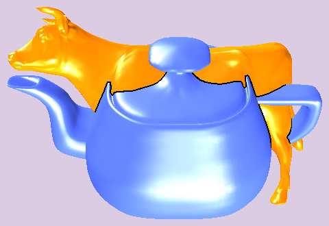
64 (a) Intersection Curve (b) Intersection Curve (c) Difference (d) Difference (e) CSG (f) Mesh (g) Surface (h) Point (i) Splat (j) Difference (k) Union (l) Difference Figure 5.3: Applications of Voxelization

65 5.5.2 Integral Properties Measurement Another application of voxelization is that it can be used to measure integral properties of solid objects such as mass, volume and surface area. Without discretization, these integral properties are very difficult to measure, especially for free-form solids with arbitrary topology. Volume can be measured simply by counting all the voxels inside or on the surface boundary because each voxel is a unit cube. With efficient flooding algorithm, voxels inside or on the boundary can be precisely counted. But the resulting measurement may not be accurate because boundary voxels do not occupy all the corresponding unit cubes. Hence for higher accuracy, higher voxelization resolution is needed. Once the volume is known, it is easy to measure the mass simply by multiplying the volume with density. Surface area can be measured similarly. But using this approach would lead to big error because we do not know how surfaces pass through their corresponding voxels. Fortunately, surface area can be measured much more precisely in the voxelization process. As we know, during the recursive voxelization process, if the recursive process stops, all the marked parameter points of a patch or subpatch (See Fig. 5.1) are points used for final voxelization. Hence all these quadrilaterals corresponding to these marked parameter points can be used for measuring surface area after these marked parameter space points are mapped to 3D space. The flatness of these quadrilaterals is required to be tested if high accuracy is needed. The definition of patch flatness and the flatness testing method can be found in [71] Performing Boolean and CSG Operations The most important application of voxelization is to perform Boolean and CSG operations on free-form objects. In solid modeling, an object is formed by performing Boolean operations on simpler objects or primitives. A CSG tree is used in recording the construction history of the object and is also used in the ray-casting process of the object. Surface-surface intersection (including the in-on-out test) and ray-surface intersection are the core operations in performing the Boolean and CSG operations. With voxelization, all of these problems become much easier set operations. For instance, Fig. 5.3(d) is generated by subtracting a cylinder from the Venus model. While Fig. 5.3(k) and Fig. 5.3(l) are the union and difference results of the cow model and the rocker arm model shown in Fig. 5.3(g). Note that all these union and difference pairs are positioned the same way when Boolean operations are performed. Fig. 5.3(j) is generated by subtracting the the heart model shown in Fig. 5.3(c), from rock arm model shown in Fig. 5.3(g). And Fig. 5.3(c) is generated by subtracting the rock arm model shown in Fig. 5.3(g) from the heart model. A mechanical part is also generated in Fig. 5.3(e) using CSG operations. Intersection curves can be similarly generated by searching for common voxels of objects. The black curve shown in Fig. 5.3(b) and Fig. 5.3(a) is the intersection curve generated from two different objects.

66 Chapter 6 Shape Design: Interpolation based In this chapter we present our interpolation based shape design technique for Catmull-Clark subdivision surfaces [67]. The new interpolation method [67] handles both open and closed meshes. Normals or derivatives specified at any vertices of the mesh (which can actually be anywhere) can also be interpolated. The construction process is based on the assumption that, in addition to interpolating the vertices of the given mesh, the interpolating surface is also similar to the limit surface of the given mesh. Therefore, construction of the interpolating surface can use information from the given mesh as well as its limit surface. This approach, called similarity based interpolation, gives us more control on the smoothness of the interpolating surface and, consequently, avoids the need of shape fairing in the construction of the interpolating surface. The computation of the interpolating surface s control mesh follows a new approach, which does not require the resulting global linear system to be solvable. An approximate solution provided by any fast iterative linear system solver is sufficient. Nevertheless, interpolation of the given mesh is guaranteed. This is an important improvement over previous methods [18] because with these features, the new method can handle meshes with large number of vertices efficiently. Although the new method is presented for CCSSs, the concept of similarity based interpolation can be used for other subdivision surfaces as well [67]. The remaining part of this chapter is organized as follows. Section 1 gives a brief review of previous interpolation methods. Our method is given in Section 2. A technique that works for open meshes is presented in Section 3. Implementation issues and test results are presented in Section Previous Work There are two major ways to interpolate a given mesh with a subdivision surface: interpolating subdivision [35, 36, 37, 57, 60] or global optimization [38, 54, 67]. In the first case, a subdivision scheme that interpolates the control vertices, such as the Butterfly scheme[37], Zorin et al s improved version [36] or Kobbelt s scheme [35], is used to generate the interpolating surface. New vertices are defined as local affine combinations of nearby vertices. This approach is simple and easy to implement. It can handle meshes with large number of vertices. However, since no vertex is ever moved once it is computed, any distortion in 60

67 the early stage of the subdivision will persist. This makes interpolating subdivision very sensitive to the irregularity in the given mesh. In addition, it is difficult for this approach to interpolate normals or derivatives. The second approach, global optimization, usually needs to build a global linear system with some constraints [59]. The solution to the global linear system is an interpolating mesh whose limit surface interpolates the control vertices in the given mesh. This approach usually requires some fairness constraints in the interpolation process, such as the energy functions presented in [54], to avoid undesired undulations. Although this approach seems more complicated, it results in a traditional subdivision surface. For example, the method in [54] results in a Catmull-Clark subdivision surface (CCSS), which is C 2 continuous almost everywhere and whose properties are well studied and understood. The problem with this approach is that a global linear system needs to be built and solved. Hence it is difficult to handle meshes with large number of control vertices. There are also subdivision techniques that produce surfaces to interpolate given curves or surfaces that near- (or quasi-)interpolate given meshes [58]. But those techniques are either of different natures or of different concerns and, hence, will not be discussed here. 6.2 Similarity based Interpolation Given a 3D mesh P with arbitrary topology, our new method [67] calculates a control mesh Q whose CCSS interpolates the vertices of P. The CCSS of Q is constructed with the additional assumption that its shape is similar to a reference surface, the limit surface of P. A shape fairing process is not required in the construction process of the interpolating surface. The computation of the control mesh Q follows a new approach which does not require the resulting global linear system to be solvable. An approximate solution provided by any fast iterative linear system solver is sufficient. Hence, handling meshes with large number of vertices is not a problem. Nevertheless, interpolation of the given mesh is guaranteed. The new method can handle both closed and open meshes. The interpolating surface can interpolate not only vertices of a given mesh, but also derivatives and normals anywhere in the parameter space of the surface Mathematical Setup Given a 3D mesh with n vertices: P = {P 1,P 2,,P n }, the goal here is to construct a control mesh Q whose CCSS interpolates P (the vertices of P, for now). The construction of Q follows the following path. First, we perform one or more levels of Catmull-Clark subdivision on P to get a finer control mesh G. G satisfies the following property: each face of G is a quadrilateral and each face of G has at most one extra-ordinary vertex. The vertices of G are divided into two groups. A vertex of G is called a Type I vertex if it corresponds to a vertex of P. Otherwise it is called a Type II vertex. Q is then defined as a control mesh with the same number of vertices and the same topology as G. We assume Q has m vertices Q = {Q 1,Q 2,,Q m }, m > n, and the first n vertices correspond to the n Type I vertices of G (and, consequently, the n vertices of P). These n vertices of Q will also be called Type I vertices and the remaining m n vertices Type II vertices. This way of setting up Q is to

68 ensure the parametric form developed for a CCSS patch [29, 70] can be used for the limit surface of Q, denoted S(Q), and we have enough degree of freedom in our subsequent work. Note that m is usually much bigger than n. The remaining job then is to determine the position of each vertex of Q. In previous methods [38, 54] the n Type I vertices of Q are set as independent variables, the m n Type II vertices are represented as linear combinations of the Type I vertices. Since m n is bigger than n, this setting leads to an over-determined system. Without any freedom in adjusting the solution of the system, one has no control on the shape of the resulting interpolating surface S(Q) even if it carries undesirable undulations. In our approach [67], instead, the m n Type II vertices are set as independent variables and the n Type I vertices are represented as linear combinations of the Type II vertices. This approach provides us with enough degrees of freedom to adjust the solution of the resulting linear system and, consequently, more control on the shape of the interpolating surface S(Q) Interpolation Requirements Recall that Type I vertices of Q are those vertices that correspond to vertices of P. Hence, each vertex of P is the limit point of a Type I vertex of Q. We assume the limit point of Q i is P i, 1 i n. Then for each Type I vertex Q i (1 i n), we have Q i = C i Q + cp i (6.1) where Q = {Q n+1,q n+2,,q m } is the vector of Type II vertices. Vector C i and constant c depend on the topology of P and the degree of vertex P i. C i and c can be easily obtained using the formula for calculating the limit point of a CCSS [29, 54, 70]. The conditions in eq. (6.1) are called interpolation requirements, because they have to be exactly satisfied. Note that the interpolation requirements in eq. (6.1) form a system of linear equations. By solving this system of linear equations, we solve the interpolation problem [38]. But in this case one tends to get undesired undulations on the resulting interpolating surface [54] Similarity Constraints Two CCSSs are said to be similar if their control meshes have the same topology and they have similar ith derivatives (1 i < ) everywhere. The first condition of this definition is a sufficient condition for the second condition to be true, because it ensures the considered CCSSs have the same parameter space. The CCSSs considered here, S(Q) and S(G), satisfy the first condition. Hence, we have the sufficient condition to make the assumption that S(Q) and S(G) are similar. In the following, we assume S(Q) and S(G) are similar in the sense of the above definition. With explicit parametrization of a CCSS available [29], it is possible for us to consider derivatives of S(Q) and S(G) at any point of their parameter space. However, to avoid costly integration of derivative expressions, we will only consider derivatives sampled at the following parameter points [65]: {(k 1 /2 i, k 2 /2 j ) 0 i, j, 0 k 1 2 i, 0 k 2 2 j } (6.2)

69 for each patch of S(Q) and S(G). In the above similarity definition, two derivatives are said to be similar if they have the same direction. In the following, we use the similarity condition to set up constraints in the construction process of S(Q). Given two surfaces, let D u and D v be the u and v derivatives of the first surface and ˆD u and ˆD v the u and v derivatives of the second surface. These derivatives are similar if the following condition holds: A different condition, shown below, is used in [38, 54]. D u ˆD u = 0 and D v ˆD v = 0 (6.3) D u ( ˆD u ˆD v ) = 0 and D v ( ˆD u ˆD v ) = 0 (6.4) These two conditions are not necessarily equivalent. Our test cases show that eq. (6.3) gives better interpolating surfaces. This is because eq. (6.4) only requires the corresponding derivatives to lie in the same tangent plane, no restrictions on their directions. As a result, using eq. (6.4) could result in unnecessary undulations. Note that eq. (6.3) requires directions of D u and D v to be the same as that of ˆD u and ˆD v, respectively. Conditions of the type shown in eq. (6.3) are called similarity constraints. These constraints do not have to be satisfied exactly, only to the extent possible. The interpolation method used in [38] considers interpolation requirements only. The method in [54] also includes fairness constraints to avoid undesired undulations and artifacts Global Linear System If the derivatives of S(Q) and S(G) are sampled at a point in eq. (6.2) then, according to eq. (6.3) and the derivative of the parametric form of a CCSS patch [29, 65], we would have (V T Q) (V T G) = 0 (6.5) where V is a constant vector of scalars whose values depend on the type of the derivative and the point where the sampling is performed. This expression actually contains 3 equations, one for each component. Replace the Type I vertices Q 1,Q 2,,Q n in the above expression with eq. (6.1) and combine all the similarity constraints, we get a system of linear equations which can be represented in matrix form as follows: D X = C where X is a vector of length 3(m n), whose entries are the x, y and z components of Q. D usually is not a square matrix. Hence we need to find an X such that (D X C) T (D X C) is minimized. This is a quadratic programming problem and can be solved using a linear least squares method. It is basically a process of finding a solution of the following linear system: A X = B (6.6) where A = D T D and B = D T C. A is a symmetric matrix. Hence only half of its elements need to be calculated and stored. Once X is known, i.e., Q is known, we can find Q 1,Q 2,,Q n using eq. (6.1).

70 The matrix D could be very big if many sample points or constrains are used. Fortunately, we do not have to calculate and store the matrix D and the vector C. Note that A and B can be written as A = D i (D i ) T and B = D i c i where (D i ) T is the ith row of D and c i is the ith entry of C. Note that the number of rows (constrains) of D can be as large as possible, but the number of its columns is fixed, 3(m n). Suppose the ith constraint (See eq. (6.5)), with Q 1,Q 2,,Q n replaced, is written in vector form as U T X = u. Then U T is the ith row of matrix D and u is the ith entry of C. Hence rows of matrix D and entries of C can be calculated independently from eq. (6.5) for each constraint of each sample point. Therefore, A and B can be accumulatively calculated, constraint by constraint. No matter how many sample points are used, and no matter how many constraints are considered for every sample point, only a fixed amount memory is required for the entire process and the size of matrix A is always the same, 3(m n) 3(m n). Note that the solution of eq. (6.6) only determines the positions of Type II vertices of Q. Type I vertices of Q are represented as linear combinations of Type II vertices in the interpolation requirements defined in eq. (6.1). Since interpolation of the vertices of P is determined by the interpolation requirements (See eq. (6.1)) only, this means as long as we can find a solution for eq. (6.6), the task of constructing an interpolating surface that interpolates the vertices of P can always be fulfilled, even if the solution is not precise. Hence, an exact solution to the linear system eq. (6.6) is not a must for our method. An approximate solution provided by a fast iterative linear system solver is sufficient. As a result, the new method can handle meshes with large number of vertices efficiently. This is an important improvement over previous methods. With the similarity assumption, the surface interpolation problem is basically a process of using an iterative method to find an approximate solution for the global linear system eq. (6.6). An initial guess for the iterative process can be obtained directly from G by scaling G properly, such that dimension of the scaled limit surface is the same as the interpolating surface. The required scaling factors s x, s y and s z for such a task can be determined by the condition that the bounding box of the scaled limit surface is the same as the bounding box of the interpolating surface. This can easily be done by comparing the maxima and minima of the vertices of the given mesh in all three directions with the maxima and minima of their corresponding limit points. The scaled mesh called Ĝ, is a good initial guess for the iterative process because Ĝ is actually very close to the control mesh of the interpolating surface we want to obtain. In our implementation, the Gauss-Seidel method is used for the iterative process. The iterative process would converge to a good approximate solution very rapidly with this initial guess. However, it should be pointed out that there is no need to carry out the iterative process to a very precise level. According to our test cases, a residual tolerance of the size ǫ = 10 6 does not produce much noticeable improvement on the quality of the interpolating surface than a residual tolerance of the size ǫ = 10 3, while the former takes much more time than the latter. Therefore a relatively large residual tolerance can be supplied to the iterative linear system solver to prevent it from running too long on the iterative process, while not improving the quality of the interpolating surface much. This is especially important for processing meshes with large number of vertices.

71 6.2.5 Additional Interpolation Requirements In addition to the interpolation requirements considered in eq. (6.1), other interpolation requirements can be included in the global linear system as well. One can also modify or remove some of the interpolation requirements in eq. (6.1). For example, if we wants the first u derivative of the interpolating surface at P i to be D u, we need to set up a condition similar to eq. (6.5) as follows: (V T Q) D u = 0 where V is a constant vector. The difference here is, this is not a similarity constraint, but an interpolation requirement. However, if we want a particular normal to be interpolated, we should set up interpolation requirements for the u derivative and the v derivative whose cross product equals this normal, instead of setting up an interpolation requirement for the normal directly, to avoid the involvement of non-linear equations in the system. Then by combining all the new interpolation requirements with the original interpolation requirements in eq. (6.1), we get all the expressions for vertices that are not considered independent variables in the linear system in eq. (6.6). Note that including a new interpolation requirement in the interpolation requirement pool requires us to change a variable vertex in eq. (6.6) to a non-variable vertex. Actually, interpolation requirements can be specified for any points of the interpolating surface, not just for vertices of P. This is possible because we have a parametric representation for each patch of a CCSS [29]. For example, if we want the position of a patch at parameter (1/2, 3/4) to be T, we can set up an interpolation requirement of the form: V T Q = T where V is a constant vector whose values depend on (1/2, 3/4). Therefore the interpolating surface can interpolate positions, derivatives and normals anywhere in the parameter space Interpolation of Normal Vectors The direction of normal vectors can be interpolated exactly by using additional interpolation requirements. The key idea is to change some similarity constrains to interpolation requirements, which means move some equations in eq. (6.5) into the linear system in eq. (6.1). Actually the direction of partial derivatives can also be interpolated by using such additional interpolation requirements. Additional interpolation requirements are conditions like eq. (6.1) that are guaranteed to be satisfied and hence, are not involved in the solving of the global linear system in eq. (6.6). However eq. (6.5) is only good for exactly interpolating partial derivatives. For exactly interpolating normal vectors, we need to interpolate the derivatives in u- and v-directions respectively to avoid the involvement of non-linear systems. For example, for a given normal vector V, whose direction is required to be interpolated at point P in the interpolating surface. Assume the derivatives at point P in the resulting interpolating surface in u- and v-directions are D 1 and D 2, respectively. Then we need to integrate the following two equations into linear system eq. (6.1): { D1 V = 0 (6.7) D 2 V = 0

72 Note that here D 1 and D 2 can be linearly represented using only the control points of the corresponding surface patch [29] and these control points are unknowns in eq. (6.1) and eq. (6.6). Because the above two equations in eq. (6.7) now are in linear system eq. (6.1), which is required to be satisfied exactly, the exact interpolation of the direction of normal vector V is guaranteed. For example, Fig. 6.1(f) is interpolated not only at vertex positions, but normal vectors at boundary vertices as well. 6.3 Handling Open Meshes (a) (b) (c) (d) (e) (f) Figure 6.1: Interpolating an open mesh: (a) given mesh; (b) limit surface of (a); (c) extended version of (a); (d) limit surface of (c); (e) interpolating surface of (a) that uses (d) as a reference surface; (f) interpolating surface of (a) with additional requirements. The interpolation process developed in the previous section can not be used for open meshes, such as the one shown in Fig. 6.1(a), directly. This is because boundary vertices of an open mesh have no corresponding limit points, nor derivatives, therefore, one can not set up interpolation requirements for these vertices, as required by the new interpolation process. One way to overcome this problem is to add an additional ring of vertices along the current boundary and connect the vertices of this ring with corresponding vertices of the current boundary to form an additional ring of faces, such as the example shown in Figure 6.1(c). The newly added vertices are called dummy vertices. We then apply the interpolation method to the extended open mesh as to a closed mesh except that there are no interpolation requirements for the dummy vertices. This technique of extending the boundary of a given mesh is similar to a technique proposed for uniform B-spline surface representation in [53]. Note that in this case, the interpolation process does not use the limit surface of the given mesh, but rather the limit surface of the extended mesh as a reference surface. Therefore, the shape of the interpolating surface depends on locations of the dummy vertices as well. Determining the location of a dummy vertex, however, is a tricky issue, and the user should not be burdened with such a tricky task. In our system, this is done by using locations of the current boundary vertices of the given mesh as the initial locations of the dummy vertices and then solving the global linear system in eq. (6.6) to determine their final locations.

73 This approach of generating dummy vertices works fine because dummy vertices only affect similarity constraints. Figure 6.1(e) is a surface that interpolates the mesh given in Fig. 6.1(a) and uses 6.1(d) as a reference surface. The above setting of the dummy vertices usually is not enough to create an interpolating surface with the desired boundary shape. Additional requirements (not constraints) are needed in the interpolation process. As explained in Section 6.2.5, a platform that allows us to define additional requirements can be created by treating the dummy vertices as non-variables in eq. (6.6). We can then specify new derivative conditions or normal conditions to be satisfied at the original boundary vertices. With the additional interpolation requirements, a designer has more control on the shape of the interpolating surface in areas along the boundary and, consequently, can generate an interpolating surface with the desired boundary shape. For example, Figure 6.1(f) is an interpolating surface of the mesh given in Figure 6.1(a), but generated with additional interpolation requirements. The interpolating surface obviously looks more like a real glass now. 6.4 Test Results The proposed approach has been implemented in C++ using OpenGL as the supporting graphics system on the Windows platform. Quite a few examples have been tested with the method described here. All the examples have extra-ordinary vertices. Some of the tested results are shown in Figures 6.1 and 6.2. Due to limited space, limit surface of the mesh shown in Figure 6.2(d) which is very simple are not shown here. For all other cases, the limit surfaces of the given meshes and the interpolating surfaces are both shown so that one can tell if these surfaces are indeed similar to each other in the least squares sense. In our implementation, only one subdivision is performed on the given mesh for each example and the first, second and third derivatives in u and v directions are used to construct interpolation constraints and build the global linear system. These derivatives are sampled at points with parameters ( k 1, k 2 i 2), i, j = 0, 1 or, and 0 k 2 j 1 2 i, 0 k 2 2 j, for each patch. That is, 9 points are sampled for each patch, which is good enough for most cases. For bigger patches one can use more sample points because patches do not have to be sampled uniformly. The mesh shown in Figure 6.2(f) is an example of an open mesh with disconnected boundaries. Figure 6.2(h) is the interpolating surface without using additional interpolation requirements in the construction process. As can be seen from Figure 6.2, all the resulting interpolating surface are very smooth and visually pleasing, except the interpolating surface shown in Figure 6.2(n). The surface has some undulations around the neck, but we do not think they are caused completely by our method. We believe this is more of a problem with the general interpolation concept. Note that the input mesh, Figure 6.2(l), has some abrupt changes of vertex positions and twists in the neck area. This is also reflected by some visible undulations in the neck area of the limit surface, Figure 6.2(m), even though they are not as clear as in the interpolating surface. An approximation curve/surface, like a spline curve, can be regarded as a low pass filter [36], which makes the given control polygon or mesh smoother. An interpolation curve/surface, on the other hand, can be regarded as a high pass filter, which magnifies

74 (a) Given (b) Limit (c) Interpolating (d) Given Mesh (e) Interpolating (f) Given Mesh (g) Limit Surface (h) Interpolating Surface (i) Given Mesh (j) Limit Surface (k) Interpolating (l) Given Mesh (m) Limit Surface (n) Interpolating Figure 6.2: Interpolating meshes with arbitrary topology.

75 undulations or twists in the input mesh. Since a limit surface is an approximation surface, it reduces the impact of abrupt vertex location changes and twists in the input mesh while the interpolating surface enhances it. This is why the undulations are more obvious in Figure 6.2(n) than in Figure 6.2(m). The new interpolation method can handle meshes with large number of vertices in a matter of seconds on an ordinary PC (3.2GHz CPU, 512MB of RAM). For example, the meshes shown in Figures 6.2(l), 6.2(a) and?? have 1022, 354 and 272 vertices, respectively. It takes 51, 14 and 3 seconds, respectively, to interpolate these meshes. For smaller meshes, like Figures 6.1(a), 6.2(i), 6.2(d) and 6.2(f), the interpolation process is done almost in real time. Hence our interpolation method is suitable for interactive shape design, where simple shapes with small or medium-sized control vertex sets are constructed using design or interpolation methods, and then combined using CSG trees to form complex objects.

76 Chapter 7 Trimming of Subdivision Surfaces and Applications In this chapter a trimming technique and its application on error controllable Boolean operations on free-form solids represented by Catmull- Clark subdivision surfaces (CCSSs) [76] are presented. The given objects are voxelized [69] using the voxelization method presented in chapter 4 first. However, different from previous voxelization based approaches, the final results of the Boolean operations in our method are represented with a continuous geometric representation, that is, our results after Boolean operations are one-piece representations of solid objects. They are represented with topologically correct mesh structure [76]. This is achieved by doing the Boolean operations in the parameter spaces of the solids, instead of the object space. The 2D parameter space is recursively subdivided until a keepor-discard decision can be made for each resulting subpatch using results of the voxelization process. This approach allows us to easily compute a parametric approximation of the intersection curve and, consequently, build a continuous geometric representation for the Boolean operation result. To make the Boolean operation result more accurate, a secondary local voxelization can be performed for intersecting subpatches. Because the voxelization process itself is very fast and robust, the overall process is fast and robust too. Most importantly, error of Boolean operation result can be estimated, hence error control is possible. In addition, our method can handle any cases of Boolean operations as long as the given solids are represented by CCSSs. Therefore there are no special or degenerated cases to take care of. Although the new method is presented for CCSSs, the concept actually works for any subdivision scheme whose limit surfaces can be parameterized. The remaining part of the chapter is arranged as follows. In section 1, a brief review of previous works related to this one is given. The process of performing Boolean operations on solids represented by CCSSs is discussed in Section 2. Local voxelization technique is presented in Section 3. Error control is given in Section 4. Implementation issues and test cases are shown in Section 5. 70

77 7.1 Related Work Performing Boolean operations is a classic problem in geometric modeling. Many approaches have been reported in the literature, such as [10, 76, 105, 111, 115, 117, 118, 119], to name a few. Currently most solid modelers can support Boolean operations on solids composed of polyhedral models or quadric surfaces (like spheres, cylinders etc.). Over the last few years, modeling using free-form surfaces has become indispensable throughout the commercial CAD/CAM industry. However, the major bottleneck is in performing robust, efficient and accurate Boolean operations on free-form objects. The topology of a surface patch become quite complicated when a number of Boolean operations are performed and finding a convenient representation for these topologies has been a major challenge. As a result, some solid modelers [105] use polyhedral approximation to these surfaces and apply Boolean operations on these approximate polyhedral objects. Although this approaches seem simple, there are always some special cases or degenerated cases [107] that are difficult to take care of. Some modelers use point (or surfel) based approaches [119] to perform Boolean operations and quite good results are obtained. However, error control is difficult in such approaches. Zorin etc. proposed a method [10] to perform approximate Boolean operations on free-form solids represented by subdivision surfaces. The main contribution of their method is the algorithms that are able to generate a control mesh for a multiresolution surface approximating the Boolean results. Most of the recent work in the literature on Boolean operations of curved models are focused on computing the surface intersection [106, 108, 110, 112, 114, 116]. However, the algebraic degree of the resulting curve can typically be very high (up to 324 for a pair of bicubic Bézier surfaces) [105] and the genus is also non-zero. Hence it is very difficult to represent the intersection curve analytically and the current methods are aimed at computing approximations to the intersection curve. 7.2 Performing Boolean Operations on Free-Form Solids Because we perform Boolean Operations on Free-Form Solids by voxelizing these solids, Boolean operations performed on three or more objects can be regarded as a series of Boolean operations performed on two objects. Therefore, here we only need to consider Boolean operations performed on two free-form solids A and B. As a result, only two cubic frame buffers are needed in the whole process, one for each object. The results of Boolean operations can share a cubic frame buffer with any of them. Once voxelization is done (See chapter 4), a volume flooding (see chapter 4) must be performed to mark the voxels located inside a given solid. After all these steps, there are three types of voxels in each cubic frame buffer: (1) inside voxels, (2) boundary voxels and (3) outside voxels. Several possible Boolean operations may be specified by the users. However, the essential process is almost the same. Here we illustrate the process by assuming the given Boolean operation is to find the intersection of two solid objects. With voxelization, it is actually quite simple to get the resulting voxels for a Boolean operation. For example, the voxels left after an intersection operation are those located inside or on the boundary of both objects. The difficult part is how to represent the resulting part

78 A 1 A2 I 1 A4 A5 A3 A6 A7 B1 B2 B4 B0 I 2 A0 I 3 B3 B7 B8 B5 B6 B (a) (b) Figure 7.1: Performing Boolean operations on 2D parameter space. properly and accurately. Traditionally the results of Boolean operations are represented just with voxels. The main disadvantage of this method is the results cannot be scaled seamlessly because of the nature of discretization. In the following, we present an approach that represents the final result with a continuous geometric representation Boolean Operations based on Recursive Subdivision & Voxelization For a subpatch of S(u, v) of solid A defined on [u 1, u 2 ] [v 1, v 2 ], we voxelize it one more time using the method discussed in Chapter 4. However, this time we do not write the voxels into A s cubic frame buffer, but look up the voxel values in both solid A and solid B s cubic frame buffers. Recall that we are performing an intersection operation of A and B. If all the voxel values of the whole subpatch in both cubic frame buffer are not outside, then this is a subpatch to keep. Subpatches of this type are called K-subpatches (subpatches to be kept). If the voxel values of this subpatch are all outside in both A and B s cubic frame buffer, then this is a subpatch to discard. Subpatches of this type are called D-subpatches (subpatches to be discarded). Otherwise, i.e., if some of the voxel values are inside, boundary and some of the voxel values are outside, then this is a patch with some part to keep and some part to discard. Subpatches whose voxel values contain all of inside, boundary and outside are called I-subpatches (intersecting subpatches). For example, the rectangles shown in Fig. 7.1 (a) are the parameter spaces of the resulting subpatches when the recursive voxelization process stops and the dashed polyline is part of the intersection curve of the two given solids in this patch s 2D parameter space. We can see that subpatch A 1 A 2 A 4 A 3 in Fig. 7.1 (a) is an I-subpatch. Note here all the marked (dark circles) adjacent points, when evaluated and voxelized, will be mapped to either the same voxel or adjacent voxels (see Chapter 4). For example, there does not exist any voxel between voxels corresponding to parameter points A 1 and A 3. Therefore, even though the intersection curve does not pass through A 1 or A 3, the voxel corresponding to the intersection point I 1 will fall into the closest voxel corresponding to parameter point A 1 or A 3. In this case, it falls into the voxel corresponding to A 1

79 An intersecting voxel is a voxel whose voxel value is boundary in both cubic frame buffers. Hence it is very easy to find all the intersecting voxels, which compose the intersection curve (but at this moment we do not know how to connect these intersecting voxels yet and will be explained shortly). For example, in Fig. 7.1(a), parameter points A 1 and B 7 are intersecting voxels. Once all the intersecting voxels are identified, a continuous geometric representation for the Boolean operation result can be generated as follows. K-subpatches and D-subpatches are easy to handle. They are either kept (for K-subpatches) or discarded (for D-subpatches) totally. For example, in Fig. 7.1(b), A 4 A 5 A 7 A 6 is a K- subpatch, hence A 4 A 5 A 7 A 6 will be output wholly in the tessellation or rendering process. For an I-subpatch, one can determine which part of the subpatch to keep by traversing all the marked points attached to this subpatch. For example, for the subpatch B 0 B 1 B 2 B 3 B 7 in Fig. 7.1(a), after a traverse of the marked vertices, it is easy to see that the part to keep is the triangle B 2 B 3 B 7. Hence B 2 B 3 B 7 will be used in the tessellation and rendering process and other region of the subpatch B 0 B 1 B 2 B 3 B 7 in Fig. 7.1(a) will be discarded. Note here the intersection point I 2, after voxelization, maps to the voxel B 7. In Fig. 7.1(b) the shaded part is the result after performing the Boolean operation in the 2D parameter space. Once we have the result of the Boolean operation in 2D parameter space, the 3D result can be easily obtained by directly evaluating and tessellating these shaded polygons. Note here we obtain not only the polygons, but also their connectivity. Hence a mesh structure can be achieved in the above process. It is the mesh structure that we can consider as a one-piece representation of the results of Boolean operations. In this stage, we have a continuous geometric representation (the mesh) as well as a discrete voxel based representation (the cubic frame buffer) for our resulting shape of Boolean operations. Because now we have both representations, a connected intersection curve can be easily constructed as well by picking boundary voxels (from the discrete voxel based representation) and traversing the mesh structure (information of the continuous geometric representation). For example, in Figure 7.1, the intersection curve (inside this patch) is A 1 A 4 A 6 B 2 B 7 B 8. The above voxelization process and Boolean operations guarantee that shared boundary or vertex of patches or subpatches will be chopped, kept or discarded in exactly the same way no matter on which patch the operation is performed. Therefore, in our approach, Boolean operations of free-form objects represented by CCSSs can be performed on the basis of individual patches Crack Prevention Due to the fact that adjacent patches might be tessellated by quadrilaterals corresponding to subpatches from different levels of the midpoint subdivision process mentioned in the above section, cracks could occur between adjacent patches or subpatches. For instance, in Figure 2.3, the left patch A 1 A 2 A 5 A 6 is approximated by one quadrilateral but the right patch is approximated by 7 quadrilaterals. Consider the boundary shared by the left patch and the right patch. On the left side, that boundary is a line segment defined by two vertices : A 2 and A 5. But on the right side, the boundary is a polyline defined by four vertices : A 2, C 4, B 4, and A 5. They would not coincide unless C 4 and B 4 lie on the line segment defined by A 2 and A 5. But that usually is not the case. Hence, cracks would appear between the left patch and the right patch.

80 Fortunately Cracks can be eliminated simply by replacing each boundary of a patch or subpatch with the one that contains all the evaluated points for that boundary. For example, in Figure 2.3, all the dotted lines should be replaced with the corresponding polylines. In particular, boundary A 2 A 5 of patch A 1 A 2 A 5 A 6 should be replaced with the polyline A 2 C 4 B 4 A 5. As a result, polygon A 1 A 2 A 5 A 6 is replaced with polygon A 1 A 2 C 4 B 4 A 5 A 6 in the tessellation process. For rendering purpose this is fine because graphics systems like OpenGL can handle polygons with non-co-planar vertices and polygons with any number of sides. However, it should be pointed out that through a simple zigzag technique, triangulation of those polygons is actually a simple and very fast process. More details about the crack prevention problem are presented in Chapter 6. Cracks could also occur if solids A and B are not connected properly in the intersecting area. For example in Fig. 7.1 (a), intersection point I 1 after evaluation and voxelization falls to voxel corresponding to 2D parameter point A 1 of solid A. If I 1 falls to voxel corresponding to 2D parameter point Ā1 of solid B, then after evaluation, S A (A 1 ) might not equal S B (Ā1) exactly. Hence crack occurs. To eliminate this kind of cracks, we cannot use the exact 3D positions evaluated from 2D parameter points for intersection point. Instead we use the center of the corresponding voxel as the intersection point. In this way, solids A and B will have exactly the same intersection positions and intersection curve as well. As a result, solids A and B can be connected seamlessly. Note that for K-subpatches, their vertices will be evaluated directly from parameter points. Only intersection points of partially kept I-subpatches are approximated by the centers of their corresponding voxels. 7.3 Local Voxelization The voxelization process presented in the above section is called a global voxelization, because it is performed for the entire object space. After all the Boolean operations are performed, a fine scale voxelization, called a local voxelization, will also be performed. The goal of the local voxelization is to improve the accuracy of the I-subpatches. For example, in Fig. 7.1(a), A 1 A 2 A 4 is used to approximate the area of the I-subpatch A 1 A 2 A 4 A 3 that should be kept. The accuracy of this approximation depends on the resolution of the global cubic frame buffer, which is always not high enough because of limited memory resource. However, we can do a secondary voxelization, which has lower resolution, but is only applied to a very small portion of the object space. As a result high accuracy still can be achieved at intersecting area. The process and the approach used for a local voxelization are the same as a global voxelization. The only difference is that they are applied to different size of the object space. In order to perform local voxelization, information about which subpatches of solid A intersecting with which subpatches of solid B must be known first. This information is very difficult to obtain in previous voxelization based methods. Fortunately, in our method, it can be readily obtained when performing the Boolean operations, as mentioned in Section If we mark these intersecting subpatches of solids A and B during the keep-or-discard test process, we would know exactly which subpatches of solid A intersect which subpatches of solid B. Once all intersecting subpatches are known, local voxelization can be directly performed for each pair of intersecting subpatches. For example, suppose subpatch p 1 of

81 object A intersects subpatches q 1 and q 2 of object B, then a local voxelization is performed on these 3 subpatches only. Their intersection curve is used to replace the intersection curve obtained using the global voxelization process. The local voxelization process is applied to every pair of intersecting subpatches of solids A and B. Consequently, more accurate intersection curve could be computed. For instance, in Fig. 7.1(a), the intersection curve A 4 A 1 will be replaced with V 1 V 2 V k, k = 10, if V i, i = 1 10 are the new intersecting voxels in the corresponding local cubic frame buffers and polygon A 1 A 2 A 4 V 1 V 2 V k will be used in the tessellation and rendering process. Similar to global voxelization, only two local cubic frame buffers are needed for local voxelization. The local cubic frame buffers can be reused for each new pair of intersecting subpatches. Hence local voxelization does not require a lot of memory. 7.4 Error Control Given an ǫ, the purpose of error control is to make sure the error of the resulting solid after performing Boolean operations using our method is less than ǫ to the one hundred percent accurate result. There are two kinds of error that might occur when our method is applied to perform Boolean operations among closed free-form solids represented by Catmull-Clark subdivision surfaces. They are discussed as follows. The first one possible inaccuracy possibly occurring using our method is the approximation of resulting solids with polygonal meshes. Because all obtained resulting solids are approximated with polygonal meshes, even although the approximating meshes are dense and are very close to the true surface, error inevitably occurs. However, the error caused by approximation of polygonal meshes can be accurately measured [68, 76]. Hence error control for this type of error is possible. The measurement of this kind of error is discussed in Chapter 6. Another source that could introduce error in the result of the Boolean operations is the voxelization process. Both the global and the local voxelization can cause inaccuracy. The kind of error caused by voxelization is easy to estimate if the resolutions of cubic frame buffers are known. For example, if the cubic frame buffer resolution is R 1 R 2 R 3 and the object space is of size X 1 X 2 X 3, then we can see that each voxel is of size X 1 R 1 X 2 R 2 X 2 R 3. It is easy to see the maximal error of voxelization is half the size of a voxel. If we perform local voxelization for every pair of intersecting subpatches, then global voxelization will not cause any error. Here we can also see why local voxelization can improve the accuracy dramatically. In local voxelization, because the size of the subpatches being voxelized are very small, even with a low resolution, the voxel size is still very small. Therefore the overall error caused by polygonalization and voxelization is the sum of the errors caused by each of them. To make error of the final Boolean operation results less than the given ǫ everywhere, the test condition in eq. (2.5) has to be changed to the following form: { d ( ū, v) + d ( û, ˆv) ǫ/2 (7.1) size of each voxel ǫ where (û, ˆv) and (ū, v) is defined the same way as in eq. (2.5). The first equation in eq. (7.1) ensures the patch (or subpatch) and its approximating polygon are both located inside

82 two quadrilaterals that are ǫ/2 away. The second equation in eq. (7.1) ensures the error caused by voxelization is not bigger than ǫ/2. Hence the total error in the whole process is guaranteed to be less than ǫ. 7.5 Test Results The proposed approach has been implemented in C++ using OpenGL as the supporting graphics system on the Windows platform. Quite a few examples have been tested with the method described here. All the examples have extra-ordinary vertices. Some of the tested results are shown in Figures 7.2. The resolution of global voxelization is for all the test examples, and the error for all of them is set to The size of each example is normalized to [0, 1] before voxelization and Boolean operations are performed. Resolutions of the local voxelization process depend on error tolerance and the given meshes. Hence resolution of local voxelization is different for each of the examples shown in Figures 7.2. For example, resolution of local voxelization used for Figures 7.2(k) and 7.2(l) is 8 8 8, while for Figures 7.2(g), 7.2(h), 7.2(i) and 7.2(j) the resolution used for local voxelization is Although resolutions used for local voxelization are different, the overall error is the same in the final results. From eq. (7.1) we can see this difference is because intersecting subpatches in Figures 7.2(g), 7.2(h), 7.2(i) and 7.2(j) have bigger size than Figures 7.2(k) and 7.2(l). In Figure 7.2, all the Difference and Intersection operations are performed on solids positioned exactly the same as in the Union operation so that we can easily tell if results of the Boolean operations are correct within the given error tolerance. For example, Figures 7.2(j) and 7.2(g) are results of Difference operation and Union operation, respectively, on solids placed in the same positions. Similarly, Figures 7.2(i) corresponds to 7.2(h), 7.2(b) corresponds to 7.2(a), 7.2(d) corresponds to 7.2(c), 7.2(f) corresponds to 7.2(e) and 7.2(l) corresponds to 7.2(k).

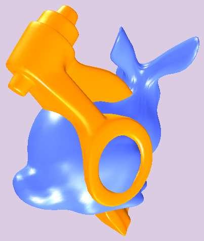
83 (a) Union (b) Difference (c) Union (d) Difference (e) Union (f) Difference (g) Union (h) Union (i) Intersection (j) Difference (k) Union (l) Difference Figure 7.2: Boolean Operations Performed on Solids Represented by CCSSs.

84 Chapter 8 Subdivision Surface based Modeling A system that performs subdivision surface based modeling using techniques that we have developed so far has been implemented. Quite a few examples have been tested. The examples show that our approaches can obtain very good subdivision based representation results. The structure of the system is shown in Figure 8.2. A snapshot of the system is shown in Figure 8.3. One advantage of subdivision surface based modeling is that one can use just one surface to represent object of any shape and any topology. A comparison of subdivision surface based representation and multi-piece representation is given in Figure 8.1. Figure 8.1(a) is the control mesh of the representation surface shown in Figure 8.1(b) and Figure 8.1(c) is the mesh of the multi-piece representation surface shown in Figure 8.1(d), where different colors denoting different parts. We can see from Figure 8.1, with subdivision surface based representation, the number of component in the representation is only one. 78

85 (a) One-piece mesh (b) One-piece surface (c) Multi-piece mesh (d) Multi-piece surface Figure 8.1: Subdivision surface based one-piece and multi-piece Representations.

86 Basic Primitives Conversion Subdivision Meshes Refinement or Direct Evaluation Voxels Voxelization Subdivision Surfaces In-Out Test Boolean Results with a Continuous Geometric Representation Joining Any Surface Sampling Dense One-Piece Representation Interpolation Irregular Meshes Adaptive Tessellation Multiresolution Analysis Sparse One-Piece Tessellation with Error Control Sparse One-Piece Representation with Error Control Figure 8.2: Structure of the subdivision surface based modeling System

87 Figure 8.3: A snapshot of the subdivision surface based modeling system.