DEPARTMENT INFORMATION ENGINEERING AND COMPUTER SCIENCE MASTER DEGREE IN TELECOMMUNICATIONS ENGINEERING THESIS. Title of the thesis

Transcription

1 DEPARTMENT INFORMATION ENGINEERING AND COMPUTER SCIENCE MASTER DEGREE IN TELECOMMUNICATIONS ENGINEERING THESIS Title of the thesis MULTI-LABEL REMOTE SENSING IMAGE RETRIEVAL BASED ON DEEP FEATURES Thesis Advisors: Dr. Begüm Demir Dr. Xavier Giró i Nieto Student: Michele Compri ACADEMIC YEAR

2 1

3 Acknowledgements In the first place,i would like to express my gratitude and appreciation to my project supervisor Professor Begum Demir and Xavi Giró for their support and persistent guidance during this thesis. I would especially to thank Albert Gil, Josep Pujal and Massimo Santoni for their help with technical problems during these last months. I also want to thank my colleagues in the X-Theses at UPC for their suggestions and help in the development of this thesis. 2

4 CONTENTS 1. Introduction 5 2. Deep Learning Historical Context Introduction to Neural Networks Convolutional Neural Networks Deep features for multi-label remote sensing image retrieval Introduction Adopted deep CNN Fine-tuning of pretrained CNN on ImageNet Multi-label remote sensing image retrieval Datasets Description and Design of Experiments Datasets Description Experimental Setup 50 3

5 5. Experimental Results Results obtained when fine-tuning is applied to single-labeled images Results obtained when fine-tuning is applied to multi-labeled images Conclusion and Discussion 62 Bibliography 65 4

6 CHAPTER 1 Introduction During the last decade, the advances of Remote Sensing (RS) technology has increased the quantity of Earth Observation (EO) data. Accordingly, huge amount of RS images have been acquired, leading to massive EO data archives from which mining and retrieving useful information are challenging. Conventional RS image retrieval systems often rely on keywords/tags in terms of sensor type, geographical location and data acquisition time of images stored in the archives. The performance of tag matching based retrieval method highly depends on the availability and the quality of manual tags[29]. Accordingly, content-based image retrieval (CBIR) has attracted increasing 5

7 attentions in the RS community particularly for its potential practical applications to RS image management. This will become particularly important in the near future when the number of acquired images will increase. Usually, a CBIR system consists of two main stages: i) a feature extraction stage, which aims to describe and characterize a set of images, and ii) a retrieval part that find correlation among images and retrieves the most similar with respect to query image. The image contents from large RS data archives depends on the performance of the feature extraction techniques in describing and representing the images. In the RS literature, several generic features have been proposed for retrieval problem, such as: intensity features [1]; color features [2][3]; shape feature: [4]-[6]. In the RS CBIR systems each RS image contained in an archive is categorized under a single label associated to a land-cover class. However, this assumption does not fit well with the complexity of RS images, where an image might have multiple land-cover classes (primitive classes) and thus can be associated to different semantic meanings simultaneously. In this thesis unlike the existing CBIR systems, multi-label learning for method has been developed for annotation and retrieval RS images from an archive ( see Chapter 4 for more details regarding the archive ). Deep learning(dl) has attracted great attention in RS for image classification problems [11][12], whereas according to our knowledge this thesis is the first work that investigates different deep learning architectures in the framework of multi-label image retrieval problems in RS. To this end, three different DL architectures are considered: 1) VGG16 [7]; 2) InceptionV3[8]; and 3)ResNet50 [9]. The first architecture taken into account is VGG16 [7], a CNN characterized by 16 layers, which are represented by stack of convolutional layers, where filter with small receptive field are used to capture information. Some of convolutional layers are followed by max pooling layer, which 6

8 aims to down sample the image, reduce its dimensionality. At top of architecture, there are three fully connected layers, which receive and combine information comes from last pooling layer to predict the output. For more details, readers are related to read [7]. To increase the performance, another deep convolutional neural network, more deeper than VGG16, has been considered. Inception V3 [8], an improved version of GoogleNet [10], contains more layers to increase the depth of model inception module, which reduces computational and memory cost with a high performance. Due to its success, ResNet50 [9], is also analyzed in this thesis. That network is mainly Inspired by VGG nets, but is also more deeper than previous Inception V3 network and use a special module, called residual model that increases performance with less parameters. For more details regarding the inception module, readers are suggested to see Chapter 3. Analyzing the performance, ResNet50 overcome the performance obtained with VGG16, hence with Inception V3, achieving best results as shown in Chapter 5. The fine-tuning approach is being considered to adapt benchmark archive images to pretrained architectures on ImageNet dataset for RS image retrieval problem. The benifits of using this way due to the fact that earlier layers contain more generic features useful to different tasks, while high level layers are more specific to the classes contained in the dataset. For that reason, last layers of the architecture are properly fine-tuned to adapt benchmark archive. To this purpose, proposed method are organized in three main stages: i) single-label and multi-label fine-tuning model; ii) features extraction; iii) image retrieval. Experiments carried out on a benchmark archive of aerial images show that the considered deep architectures provide high retrieval accuracy in terms of both single label and multi-label settings. In addition, comparison with performance obtained by neglecting fine-tuning models emphasizes the benefits of using fine-tuning approach. 7

9 The remaining part of the thesis is structured as follows: Chapter 2 is devoted to give an overview about deep learning concept, starting from historical facts, whereas is explored the milestones stages of deep learning is explored, starting from perceptron, passing through multi layer perceptron, up to convolutional neural networks. Chapter 3 is related to the core of this thesis, which describes step by step the procedure followed to achieve the results, from fine-tuning the module to image retrieval. Chapter 4 is devoted to describe archive content and experimental set-up, while experimental results are shown in Chapter 5. Last chapter is devoted to conclude, where the thesis results are resumed and analysed. 8

10 CHAPTER 2 Deep Learning Deep Learning(DL) is a branch of machine learning related to algorithms inspired by the biological brain system called artificial neural networks. Its success is due to the fact that it is able to learn automatically data efficiently, as opposed to most traditional machine learning algorithms, such as Support Vector Machine ( SVM), which require intense time and effort on the part of data scientists. Specially during last years DL has made a big impact on computer vision tasks, overall for pattern recognition, such as image classification and object recognition. Advances in hardware have made it possible to tackle problems with deep neural networks in a reasonable amount of time and amount of available labeled data have lead deep learning is demonstrated its efficiently. Its ability to self-thought data lies in the change that, iteration by iteration, DL optimizes parameters that it needed to reach the scope. Thus, it can learn complex, 9

11 hierarchical and also different data, even if original domain of dataset is different, as this thesis proposed 2.1 Historical Context In 1958, the psychologist Frank Rosenblatt proposed one of the first artificial neural networks, called perceptron, which combines linear weighted inputs to resolve binary classification problem.the earliest deep-learning-like algorithm was trained by Alexey Grigorevich Ivakhnenko in 1965, where layer did not depend on previous one and to propagate information was used statistical method to obtain best features and forward them through the network. The concept of backpropagation of error evolved in 1970s thanks to Linnainmaa in his master thesis that included FORTRAN code for backpropagation but did not include its application to neural networks. Rumelhart, Hinton, and Williams proofed in 1985 that backpropagation in neural networks could yield interesting distributed representations because algorithm is able to automatically learn the parameters of the network. Few years later, in 1989, Yann LeCun shows the first practical demonstration of backpropagation at Bell Labs, using convolutional neural network (CNN) together with backpropagation to classify a handwritten digits (MNIST) problem. Despite the progress, neural networks were not taken into account given the computational time problem, due to poor computational power, and the quantity of data needed to training stage, researcher started focusing on other machine learning methods, such as Support Vector Machines (SVM). Significant evolutionary step for Deep Learning took place in 1999, when computers started becoming faster at processing data and GPUs (graphics processing units) were developed. Faster processing, GPUs processing pictures, increased computational speeds by 1000 times over a span of 10 years. 10

12 One of turning point of DL happens in 2006 when Geoffrey Hilton et al [22]A fast learning algorithm for deep belief nets to demonstrate empirically that initializing the weights of this network using unsupervised models could produces much better results than the same network initialized with random weights. From this moment, the researcher community started to pay more attention on DL. The only part that missed to proof the efficiency of DL was data quantity. In 2007, Fei-Fei Li started to collect images from Internet to compose ImageNet,dataset of 14 million labeled images using for machine learning research, overall to train and test neural networks. Few years later, in 2012, Alex Krizhevsky, Ilya Sutskever, and Geoffrey Hinton with Deep Convolutional Neural Network won ILSVRC (ImageNet Large-Scale Visual Recognition Challenge), reached the best error rate of the competition. This success showed the power of these models dealing with images when they can be trained efficiently using graphics processing units (GPUs) with tons of labeled data. 11

13 2.2 Introduction to Neural Network Perceptron Neural Networks (NNs), also knows as Artificial Neural Networks(ANNs), are inspired by biological neural networks. The human brain is composed by large number of Figure 2.1: Representation of a biological neuron. dendrites detect signal that Cell Body process and Axon send to other neuron[23] neurons, 100 billion units called neurons, which each one is composed by a cell body that catch information from dentries and communicate with other cells of other neurons through axos. 12

14 The basic unit of ANNs, neuron, is represented by using a model called perceptron developed by Rosenblatt in It performs linear combination of the incoming inputs, which has associated weight that measure the importance with respect other inputs. Then, the process continued through an activation function to obtain the output. Figure 2.2: Graphical representation of perceptron. Perceptron, which is shows in the Figure 2.2 above, takes set of inputs, where xn belongs to R, which have associated a set of weights, where wn belongs to R. The core of the neuron is split into two parts: first one devoted to sum the contribution comes from each weighted input plus bias ( ) ; instead of the other one, called activation function(af), is devoted to thresholding the result comes from the sum. In this case, as figure 2.2 suggest, AF is a step function that produces binary output. Perceptron is limited due to some factors. First of all, output returns 0 or 1, so it can be apply only to binary classification problem.then, in addition, the complexity of system allow only to solve very simple problem.to exceed the limitation of the binary output, it was introduced another popular activation function, Sigmoid. That function allows to resolve regression problem, instead of just a classification problem. The output returns real value, between 0 and 1, instead of 0 or 1. 13

15 More generally, activation function takes as input a number and apply certain mathematical function on it. The success of sigmoid have drives people to investigate around find out other activation functions to increase the performance of network. Some of them, including sigmoid, are shows below. Sigmoid : Non-linear function which well approximate neuron activation. It takes real input number and return real number between 0 and 1, to see if the neuron is fire or not Figure 2.3: Sigmoid function Hyperbolic Tangent : Non-linear function that takes real input number and return output between range [-1, 1] 14

16 Figure 2.4: Hyperbolic tangent function ReLU(Rectified Linear Unit) : function that squashes depending if input value is negative or positive. In first case the output result 0, instead of second case, the output is equal to the input. Figure 2.5: ReLU function 15

17 2.2.2 Neural Network and Backpropagation algorithm Considering that instead of building a simple neuron,perceptron, with one neuron and one activation function, build a network with many neurons can be built, where the output of a neuron could be connected to the input of another one and the last one is connected with an activation function. In this way a neural network is created. Surely, the architecture of network can have different number of neurons, number of layers and also number of outputs. Figure 2.6: Graphical representation of Multi Layer Perceptron (MLP) 16

18 The Figure 2.6 shows a simple feedforward neural network, where the blue circle represent the input of the network and orange circles denoted neurons into the network. Furthermore the circles containing +1 denoted bias term. As figure suggests, neurons are grouped on columns without being connected one to each other. This form of grouped neuron is called layer. Each layer can have variable number of neurons, but must have at least one. Layers between input layer and output layer are called hidden layers, because its value is not observable during training phase. Given a set weights values and bias terms, the scope of the network is takes the best possible decision at output. Particularly, the output of each neuron,denoted as, is computed as follows: and the final decision is computed take into account the final output of penultimate layer: 17

19 This phase is called forward propagation, where parameters are fixed and the output is computed as show above. So, now the performance of the network can be evaluated computing the error between target and the output of the network, the training sample related to weight by using squared error function. The overall cost related to all M training samples is given by the normalized sum of each single error, as follow : To achieve good performance of the neural network the error has to be minimized, to reduce the gap between target and predicted output. To reach this result the weights and bias have to been tuned correctly. An efficient way, widely known in literature, is using the gradient of cost function to have information related to the direction in which we have to optimize. Considering weight, its update value is obtained as: 18

20 where represent the partial derivation of cost function and represent the learning rate. It indicates how quickly weights are updated considering partial derivative. Learning rate could be constant or could change in each iteration, following, for example in this thesis, a decrease exponential curve. A more detailed description of learning rate will be discuss in the next section. To increase the computational efficiency of the method, the gradient is computed as average gradient of n samples. They are called mini-batches in case we are using stochastic gradient descent (SGD), where standard number of mini-batches are 32. The computation of the gradient is computationally very expensive. For that reason Rumelhart et al.[25] introduce a powerful and fast algorithm called Backpropagation able to back propagate error through the network, starting from the output layer. For more details and exhaustive explanation of the algorithms, the readers are invited to consult [25]. 19

21 2.3 Convolutional Neural Networks Convolutional neural networks (CNNs) belong to Neural networks (NNs) family, that is previously described. A peculiar of these NNs is the convolutional operation applied Figure 2.7: General representation of Convolutional Neural Network (CNN) [26] to input data, which have demonstrate very good performance for many computer vision tasks, overall for image recognition and classification. As we already know, a neural network receives an input and process it through hidden layers to obtain desired output. Each neuron is connected to all neurons of previous and next block, but does not share any information with neurons that belongs to its same layer. The final layer collect all information that have been forward propagate through the network by other layers and take the final decision. To better understand the transition from NNs to CNNs we have to take into account images as inputs. An image is a representation of visual information made up by pixels,where each one contains a number related to the color intensity. A standard color model is RGB ( Red-Green-Blue), which combining these three primary colors to produce a real images. We can image them as three 2D stacked matrix,one over each other 20

22 Figure 2.8: Graphical representation of stacked RGB image So, taking into account these information, we know that an image has a size of 3*N*N ( 3 channels, N wide, N high), means that number of parameters for a single neuron of NNs. Suppose it N = 64, are 3x64x64 = weights, that are still manageable. The problem occurs when we have a lot of neurons, because the number of parameters increase very quickly, reaching the overfitting problem. In CNNs, architecture is suitable to manage images, because layers are arranged data in 3D (height,width,depth) instead of 2D (height,width). CNNs Take a 3D input volume and returns a 3D output. A peculiarity of CNNs is also its architecture, in which it is organized by stacking three main layers that make three different functions : Convolutional layer, Pooling layer and Fully-connected layer. 21

23 2.3.1 Convolutional Layer The convolutional layer(cl) is the main block of the architecture, in which the heavy operations of the network occurs. The first CL receives input image [height,width,depth ] and applies a series of convolutional filters to it. Each filter has small size, but at same time, works to full depth dimension of the image, processing dimension by dimension. For example, if input image is RGB, the filter is applyed to each of 3 component. The output of each filter is composed by 2D activation map, which contains the value obtained from convolution between filter and image at any position of it. Then, if we suppose that for first CL there are N filters, we will have N activation maps that produce the output of the block. To better understand, let us assume that the size of input image is 64x64x3 and each neuron has size of 5x5, so each neuron will have size of 5x5x3 = 75 weights, +1 for bias. The output size depends on 3 hyperparameters of the filter: depth, stride and zero-padding. The first parameter is not to be confused with depth of image. Depth of architecture is related to the number of concatenated filter containing in a layer, as Figure 2.10 shows. Each of neuron is looking for something different in the input image, like a color or corner edge, in order to be activated. We will take into account only the activate neurons. The second parameter, stride, is related to filter shift over entire image during convolutional step. For example, if stride = 1, means that filter, after applied at a position, is moving just of a pixel to be applied again. The follow image, show an example with stride = 2. 22

24 Figure 2.9: Visual representation of filter with stride = 2 The third and last hyperparameter, zero-padding, allows to add zeros at input image in order to control the output size, in order to preserve spatial size of the input. A operational computed by a filter could be described as follow Figure 2.10: Visual representation of convolutional filter with depth = 5 On left side there is the input volume composed by three 2D matrix stacked one on each other. On right side there is the convolutional layer, where each filter, of size 2*2( receptive field), is represented by a yellow or purple neuron and depth columns of layer is equal to 5. The output is obtained only from neurons that are activated. 23

25 2.3.2 Pooling Layer Pooling operation is used in convolutional neural network to reduce number of parameters, hence it decreases computation in the network. Pooling is a downsampling operation where a filter is apply to whole image to reduce its dimension along height and width, without modifying depth component. Given a filter, usually of size 2x2, the operations applied to replace the 4 numbers with just one could be : max pooling, average pooling or L-2 normalization pooling. The most common is max pooling, where filter takes the highest value among 4 values. A general and a max pooling examples are shown below. Figure 2.11: (a) show visual representation of pooling operation and show numerical representation of max pooling operation[26] 24

26 2.3.3 Fully-connected Layer The last step of CNNs is to combine high-level features, which comes from convolutional and pooling layers in order to classify images or, more in general, learn non-linear relations among features. The layer that perform this combination is called fully-connected layer. As the name suggested, all neurons of that layer are connected to all neurons of previous one to collect all information and send them to another fully connected layer or produce output values. The most common use of FC layer is to image classification task, where the number of neuron correspond to number of classes that we want to classify. The example of Figure 2.12 shows part of CNN, where there are a convolutional or pooling layer and three FC layers. The last one is composed only by four layer, that represent the output of each class. In this case, each neuron is associated a sigmoid function, that returns probability associated for each specific class. Figure 2.12: Visual representation of last part of a CNN. Last fully-connected layer represent the output of CNN.[26] 25

27 CHAPTER 3 Deep Features For Multi-Label Remote Sensing Image Retrieval 3.1 Introduction This chapter is devoted to describe contributions in this thesis, where the aim is to evaluate CBIR for remote sensing images by using deep features. First part of this chapter is focused on CNNs, by describing their architectures and peculiarities. First illustrated CNN is AlexNet[3], which is not taken into account for this thesis, but it is mentioned because the other architectures have been inspired. The chapter continues with introduction and explanation of the fine-tuning strategy, starting from its definition to its application on single-label and multi-label classification. In addition a description of CNN training phase is added to give more clear and logical motivation of fine-tuning. Last part regarding the purpose of this thesis, remote sensing image retrieval. 26

28 In this section the strategy to obtain similarity among images is analyzed by explaining how features vectors are related among them and how images are ranked. 3.2 Adopted Deep CNNs This section describes CNNs in chronological order, from AlexNet [11] which presented in 2012 to ResNet-50, which has taken part of literature from Each of them is described by analyzing the architecture and its peculiarities (i.e. each component or structure that made it famous). As already mentioned in the introduction, AlexNet [11] is described because it has inspired the CNN developed after it, which are adopted in my work. In addition, a demo of these three architecture is available online. [15] AlexNet The first CNN that became famous was AlexNet [11], which won the 2012 ILSVRC[15] (ImageNet Large-Scale Visual Recognition Challenge), a prestigious challenge in Machine Learning field. It was the first architecture that proof the power of CNN in context of pattern recognition, become state-of-art not only in image classification but also object detection, object recognition,human pose estimation and so on. 27

29 Figure 3.1: AlexNet trained on ImageNet[11] The architecture is made up of 5 convolutional layers, max pooling layers, dropout layers and 3 fully connected layers. In addition with classical layers, here there are dropout layer, which is regularization technique to reduce overfitting, a way to perform model average in neural network. For more detailed information related to Dropout, readers are invited to read[13]. Figure 3.3 shown two parallel flows, one up and the other down. The reason is due to the fact that the process to train ImageNet dataset was computational high, thus they have decided to split training phase onto 2 GPUs. Still considering the image, input image is processed first through convolutional layer, then a max pooling layer, thus into Dropout layer and at end trough FC layer, where ReLU was used for first time. That activation function was introduced to decrease training time with respect to use tanh activation function VGG-16 VGG-16 [13] is a specific architecture of VGG networks, where the number of weights layers are 16. It perform almost the same perform of VGG-19[13], which won ILSVRC[12]

30 VGG has increase number of layer, from 8 weight layers to 16, and introduced a better hierarchical representation of visual data by using smaller filter size than AlexNet, in fact filter size in first convolutional layer are 3x3 and 11x11, respectively. In addition stride and padding are equal to 1 and are the same for all convolutional layers. This setting of parameters has exceed the performance of the state of the art lead to perform great results during ILSVRC 2014 challenge. Figure 3.2: VGG-16 trained on ImageNet[14] As figure 3.2 shown, architecture is organized in 5 blocks, in which first four blocks contain max pooling layer and convolutional layers, followed by ReLU function. An interesting characteristic of VGG-16 is that the depth of volume increases due to the 29

31 increasing number of filter in each layer, resulting in a double number of filter after each max pooling. Last part of architectures, which are highlighted with light-blue color in Figure 3.4, contain flatten vector of 4096 elements that are successively connected to FC layer having 1000 elements and softmax activation function. These number of neurons correspond to total ImageNet classes Inception V3 Inception V3 [16] is a revision of GoogleNet [7], also called Inception V1,which has contributed reducing 12 times the number of parameters with respect to state-of-the-art, thanks to the concept of inception module. Figure 3.3: Inception module of GoogleNet [7] Inception module applies different convolution and max pooling to same input, at same time, in order to have multi-level features and combines them at the end of the 30

32 module. To compute them GoogleNet uses three different filter of size 1x1, 3x3 and 5x5. Furthermore, filters blocks colored as yellow were introduced to reduce dimensionality. The researcher noticed that there was a problem of internal covariance shift, which means that when data flows through the network, weights and parameters change data values, those could result too big or too small. To overcome this problem Sergey et al.[17] introduce Batch normalization, which normalize data after each batch. This new version of GoogleNet is called Inception V2. To scaling-up the network, the team of Sergey, factorize 5x5 convolutional layer into two consecutive 3x3 convolutional layer, created a new version of the network called Inception V3. its inception module can be represented as follows : (a) (b) Figure 3.4: (a)inception module of Inception V3 and (b)two concatenate filters 3x3 As Figure 3.6 well represent, the differences with respect Inception module of Googlenet, is the replacement of filter 5x5 with two filters of size 3x3. The reason stem 31

33 from the fact that by reducing the computational cost consequently we reduce the number of parameters, having a fast training. In addition we can factorize again the filter from nxn into nx1 and 1xn Figure 3.5: (a)inception module of Inception V3 and (b)two concatenate filters 1x3 and 3x1(b) Figure 3.6: Architecture of Inception V3 [18] 32

34 As figure 3.4 shows, the architecture is composed by 11 inception modules, where 7 of them are already described above. For more detailed information related to other parts of architecture, the readers are invited to see [10] ResNet-50 Microsoft ResNet [19] is a very deep CNN, with 152 layers. It has become popular since 2015, when it won both ILSVRC[15] and COCO[14] challenges in five main tasks, becoming the new state-of-art. As name suggests, version of ResNet-50 contains 50 layers. Its use in this works, instead of other deeper versions of ResNet, is justify in the next chapter. For this section I just show a reduce architecture to explain the main concepts of this network, without shows the ResNet-50 architecture due to its huge number of layers. For more detailed about it, the readers are refered to link mentioned in first paragraph of section 3.2. To make the network deeper an intuitive idea could be simply stack layers. Unfortunately, this solution lead to reach higher training error with respect to state-of-art. A properly way to stack layers improving the performance is perform an identical mapping to output of next layer, as it shown in following figure : 33

35 Figure 3.7: Residual block [19] Suppose the input, desired underlying mapping and the residual mapping. Then last term is obtained in the following way : To obtain the desired mapping we have to just add,which perform identical mapping. So, instead of adding a different layer we replicate the previous one in order to be sure to achieve same input value. The connection between input and output is called shortcut connection [13]. The advantages, further to obtain is that none parameters are adds and the complexity does not increase. When layer size changed a zero padding is adding in order to avoid that number of parameters increased.the most popular ResNet version contains 152 layers, a huge architecture that it is omitted in this explanation for graphical dimensionality problem. 34

36 Figure 3.8: ResNet baseline architecture [19] 35

37 Figure 3.9 summarize what is explain above, where ResNet-34 was the first version of actual architecture. In the middle there is just a stack layers architecture, which performing worst result with respect to state of art. On right side there is the same architecture but with residual module added. 3.3 Fine-tuning of Pretrained CNNs on ImageNet Nowadays, most of researcher do not train whole CNN starting with random weights initialization because it requires a lot of time, which depends on computer resources, and huge amount of data, which is not always available. Generally, it is common to take a pretrained CNN on large dataset ( usually on Imagenet [12] ) in order to have already weights initialized. Before entering into detail with fine-tuning method, it is appropriate give an overview about training phase. First of all, we have to choose an architecture to train the data, which have to be splitted into two dataset : one for training phase and one for test phase. The first one in turn could be splitted into training dataset to tune properly the weights and bias, and validation set, which is useful to qualitatively evaluate the performance of the network. Furthermore, to train properly a network we need a huge amount of data, which quantity depends on number of classes that we want classify and their content complexity. For example black vs white classification images requires less data than classifying different kind of flowers. Thus, given a image training dataset at input of CNN, each image is processed through all layers and classified. Once classified, the output back forward the error through network in order to update the weights, as explained in Chapter 2, with respect to images just processed. Thus, after have choose the architecture and initialize the 36

38 weights, we can therefore proceed to fine-tune weights with respect to our data, which can be applied by using different strategies. The first one consists of removing the last fully-connected layer and substitute with another one( refers to figure 3.1), with number of neurons are related to number of classes or objects that we want to classify. Next step is to train only this FC layer with our data, extracting features ( size of them depends on architecture) from last layer before classify images. Another strategy consists not only to replace a classifier, but also fine-tune the weights in the previous layers. In this way we freeze the weights, so they do not change, all weights excepts which are contained in layers that we fine-tuned, as shown in Figure 3.2. It can be possible fine-tune whole network, but it increase the risk of overfitting. Thus it has to find a tradeoff between fine-tuning and our amount of data. Figure 3.9[21]: Visual Representation of fine-tuning CNN where classifier are substituted 37

39 Figure 3.10: Visual Representation of fine-tuning CNN where classifier are substituted Fine tuning is applied to last layers due to the fact that earlier layers contains more generic features (e.g.:edge,simple color, curves), which are useful for many tasks. The choice of this strategy compared to a random weights initialization is due to the fact that gradient descent algorithm starting point tends to be much closer to optimum point, thus large number of iterations and overfitting by using small dataset are avoided. Figure 3.1 and Figure 3.2 shows above, represent the two different fine-tuning strategies, where, in the first one, only classificator is replaced and trained, and in the other one where, instead of just to replaced and trained a classificator, the weights of one or more layers are freezed. 38

40 3.3.1 Fine-tuning with single-label images Let M full-color Remote Sensing (RS) images with 3 color components, RGB. Define a set of M images, where in turn is splitted into two dataset: that represent training dataset and the other one represents test dataset. In this case each image is associated to a single label class, belong to. The details related to single label class are reported in chapter 4. To better understand the section, it is organized in two areas: The first one called preprocessing, which describes all operation applied to images before to fine-tune the model and the other one, called fine-tuning deep neural network, which aims to explain how models are fine-tuned. Preprocessing phase Before training the model, it is fundamental to apply preprocessing techniques in order to avoid distortion information. Thus it allows a correct and easier evaluation of data through the network. First of all, each image is converted into a vector and resize from its original dimension in order to have equal size of all images. Furthermore, zero mean value and variance normalization are applied to each image. Mean values of each image is subtracted to center, from geometrical point of view, the cloud of data along origin of dimensions. 39

41 The second preprocess technique, variance normalization, is employed to have same distribution of data along every dimensions, so to allow that data are better comparable. Figure 3.4: mean subtraction and normalization data Figure 3.4 shown above represent the case in which : On left the original distribution of the data, in the middle the distribution with zero mean subtraction and on right side, the normalization distribution along every axis. fine-tuning deep neural network Once data is ready to be processed, the next step is to upload the labels, which are later associated to each image, and to convert them into array before to fine-tune the network. First of all, we have to i) choose an architecture among [13][16][19], ii) upload its original weights, which are obtained from ImageNet[15] dataset. Then, we can proceed to fine-tune weights of our model. The choice of how many layers should be freezed is relative to the quantity of available data, which means that if we have huge training dataset we can fine-tune more layers with respect to have small one. 40

42 The training dataset is not so rich to fine-tune many layers. In addition, the number of freeze layers depends also on kind of architectures. First step to fine-tune an architecture is replaced classifier part with new one. In our case, in order to compare the results, same classifier is applied to each of them, which is formed by global average pooling, followed by batch normalization layer and fully-connected layer with 21 outputs and sigmoid as activation function. Hence, the classifier, which is initialized with random weights, has to be trained with our data. So, all layers of architecture have to be freezed. After completing this step, we drive to fine-tune weights in some layers of last blocks of the model, in according to their architecture. Following the order of section 3.2, VGG-16 is composed by 5 blocks, where from last one weights are freezes and model fine-tuned. Following figure 3.5 and 3.6 highlight the part of the network which are fine-tuned. Notice that in these images the sequence after highlighted part does not have to be considered, because correspond to old classifier. Figure 3.5: Green circle highlighted layers fine-tuned of VGG-16 41

43 For the second architecture, Inception V3, the weights are freezed from 9th block over 11, where each block is composed by combination of convolutional layers, batch normalization layers and merge layers, Figure 3.6: Green circle highlighted layers fine-tuned of Inception V3 The last architecture, ResNet50, contains 16 blocks, where each one composed by convolutional layer, batch normalization and ReLU. The output of each block is merged with the input of itself. To fine-tune this architecture first 14 blocks are freezed and only the weights of last two blocks are trained. As already motivated above, the architecture of ResNet 50 is very huge to show, for that reason it is omitted.a very good visual representation of the block is shown in [15]. 42

44 3.3.2 Fine-tuning with multi-label images Let us define as multi-label set, where each label correspond to a relevant characteristic presented in the images. The process to fine-tune pretrained model is the same one explained above, so image are normalized and then use to fine-tune the model. The difference with respect to previous case are labels, in fact in this section each image is associated to a vector of multi-labels. In addition, since that number of multi-label are different to number of single label classes, the classificator is changed to fill up this diversity. The reason of this strategy is due to the fact that to evaluate the performance will be used multi-label associated to each of test image, which belong to test dataset. Multi-label contains more information than single label class, because they are related to content present in each image, instead of just the class which image belongs. 3.4 Multi-label remote sensing image retrieval This section explain how most similar images are retrieval giving at input a query one. First of all, instead of fine-tune the model, features are simply extracted from the original model to have a baseline. 43

45 features extraction without fine-tuning In this case input test images are kept as input and processed through the network until reach last layer before classifier, where it is correspond to average pooling layer. Proceeding step by step, images are converted to vector and normalized as explained in preprocessing phase of Section After that, the features are extracted from average pooling layer, which can have different dimension in according to different architecture [13][16][19]. Once features are obtained, they have to be normalized in order to prevent overfitting, (thus to make better prediction). In details, a common method widely know, which is L2 normalization, is used where Once features are normalized, they are ready to be compared. In literature, many metrics have been developed to compute distance between two vectors. The most common one is cosine similarity, which as name suggest, use the property of cosine to find relation among vectors, so it not only takes into account magnitude, but also direction. 44

46 Figure 3.7: Cosine similarity with relative formula For example suppose that building compare 10 times in a image and 1 in another one; the magnitude related this label will be high for the first one and low for the second one, but the angle will be small. Feature vectors related to each test image are now comparable among them. Thus, for each query, images are sorted in decreasing way, from most similar to less like image. In this subsection the process to extract and compare features is the same of previous one. The difference with respect to extraction without fine-tuning, are the weights, which are fine-tuned. 45

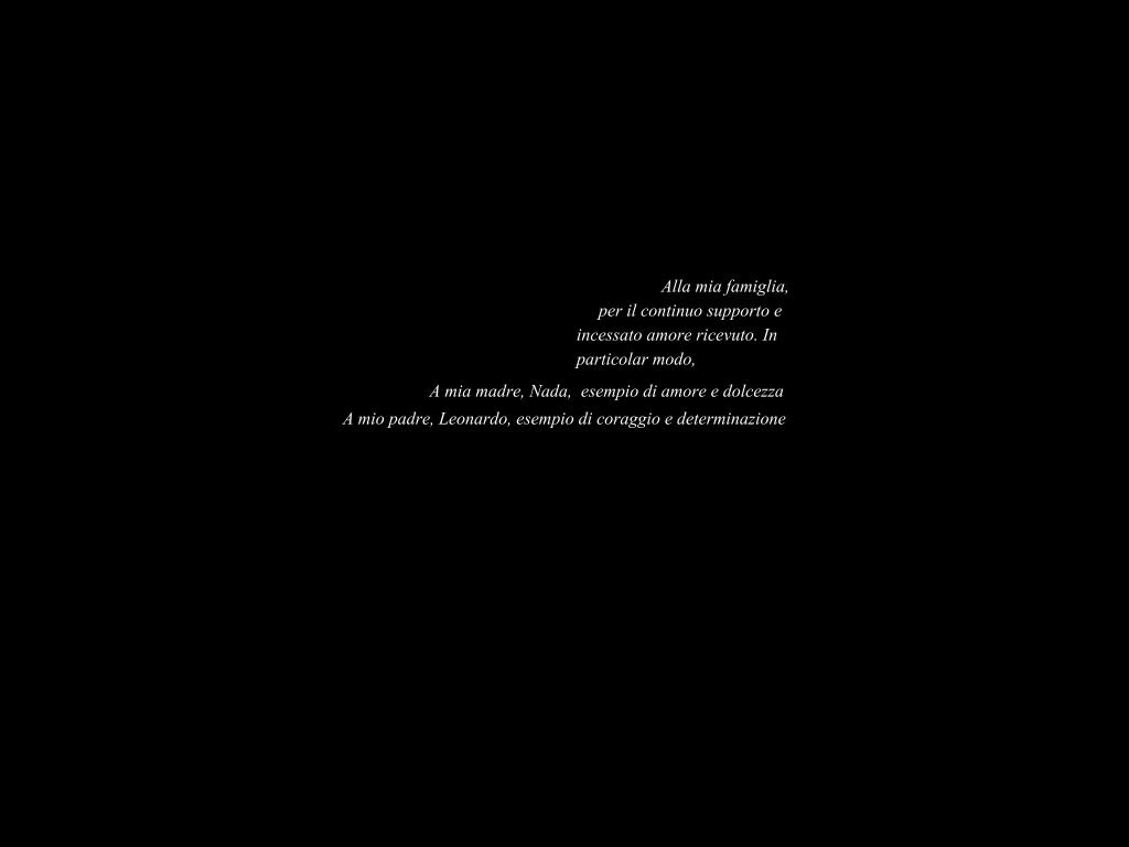
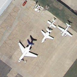
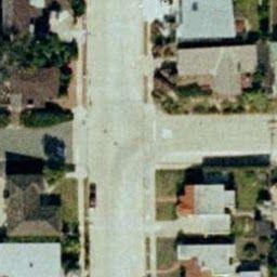
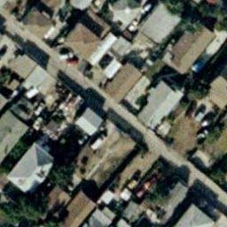
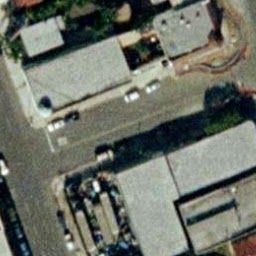
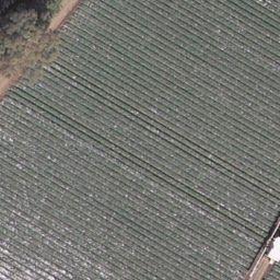
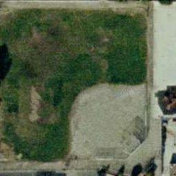
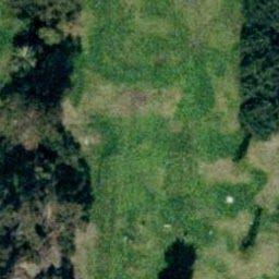
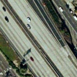
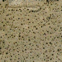
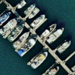
47 CHAPTER 4 Dataset Description and Design of Experiments 4.1 Dataset Description To evaluate performance of retrieval system, experiments have been conducted on UC Merced Land Use dataset that is free available in[28]. This archive contains 2100, where each of them has: i) single label; ii) primitive class labels. The images grouped in the following 21 high level classes: agricultural, airplane, baseball diamond, beach, buildings, chaparral, dense residential, forest, freeway, golf course, harbor, intersection, medium residential, mobile home park, overpass, parking lot, river, runway, sparse residential, storage tanks and tennis court. for each image are associated two or more multi-labels, which are : airplane, asphalt, buildings, bush, cars, court, dock, field, grass, road, runway, sand, sea, ship, soil, tanks, trees, water. Follows Figure 4.1 shows an example related to each category while Table I shows the relation between single label and multi-labels. 46

48 47

49 Figure 4.1: First images of each classes presented in UC Merced Land Use dataset. (1) agricultural (2) airplane (3) baseballdiamond (4) beach (5) buildings (6)chaparral (7) denseresidental (8) forest (9) freeway (10) golfcourse (11) harbor(12) intersection (13) mediumresidential (14) mobilehomepark (15) overpass (16) parkinglot (17) river (18) runaway (19) sparseresidental (20) storagetanks (21) tenniscourt 48

50 TABLE I : Single Label Classes and Multi Label present in each of them Category names Agricultural Airplane Baseball Diamond Beach Buildings Chaparral Dense Residential Forest Freeway Golf Course Harbor Intersection Medium Residential Mobile Home Park Overpass Parking Lot River Runway Sparse Residential Storage Tanks Tennis Court Associated Multi-Labels Field, Trees Airplane, Cars, Grass, Pavement, Buildings Grass, Trees, Buildings, Bare-soil, Pavement Sea, Sand, Trees, Grass, Pavement, Cars Buildings, Cars, Pavement, Trees, Grass, Bare-soil Bare-soil, Chaparral Buildings, Bare-soil, Trees, Cars, Grass Trees, Grass, Buildings, Pavement, Cars, Grass, Trees, Bare-soil, Chaparral Trees, Bare-soil, Pavement, Grass, Sand Ship, Dock, Water, Grass, Buildings Trees, Pavement, Bare-soil, Cars, Buildings, Grass Buildings, Trees, Grass, Cars, Bare-soil, Pavement Mobile-home, Cars, Trees, Bare-soil, Pavement, Grass Pavement, Cars, Bare-soil, Grass, Trees Pavement, Buildings, Cars, Bare-soil, Grass, Trees Water, Trees, Bare-soil, Buildings, Grass, Send Pavement, Sand, Grass, Bare-soil Buildings, Grass, Bare-soil, Trees, Cars, Field, Pavement, Chaparral Tanks, Bare-soil, Trees, Grass, Buildings, Sand, Cars, Pavement Court, Grass, Trees, Road, Buildings, Cars, Pavement, Bare-soil 49

51 4.2 Experimental Setup The framework chosen for this work was TensorFlow[19], that is a deep learning library written in python and developed by Google. Since that TensorFlow was recently provided online, and compatibility problem have been occurs that drive me to change framework. Thus, for this thesis I used a widely known deep learning framework, Keras[20]. It is capable running to both TensorFlow or Theano, but for technical reasons, mentioned above, the back end system used is Theano. The performance of the models are evaluated by using Matlab since that metrics provided( see Chapter 5) are developed on it. Furthermore, the tools is suitable to visualize and manage numerical information. To achieve results obtained, different parameters of the model are set properly. Their name and relative values are shown in Table II. TABLE II : Parameters setting Parameters Values Training/Test Images 1680/420 Learning Rate Initial/Final 0.001/0.01 Weights Decay Initial/Final 0/ Optimizer Initial/Final SGD/Adam 50

52 TABLE III : Baseline experiment without fine-tuning Architecture Layers Fine-tuned Total Layers( without classificator) VGG Inception V ResNet In Table III number of layers that are selected with respect to Keras documentation. They could be: input, padding, pooling, activation, merge, batch normalization or branch. For more detailed information, readers are invited to see[20]. In testing phase, after images are classified, we proceed to save, for each image, its relative feature vector obtained from output. Its dimension depends if the experiment is done on single-label classification, where the output vector has size 21, or multi-label classification, where output vector has size 17. It is worth nothing that another solution previously adapted. In this solution the features was extracted from last pooling layer, but as results proof in Chapter 5, performance are better when we take features vector from the output. 51

53 CHAPTER 5 Experimental Results This section is devoted to show performance obtained applying deep learning on UC Merced Land Use dataset. Experiments was done considering two different classification strategy: i) one in which each image is associated to a single label and; ii) other one where for each image are associated multi-labels. Furthermore, experiments without fine-tuning are shown, to emphasize the advantage of using fine-tuning on pretrained deep CNNs.To evaluate the performance we used three metrics: Accuracy, Precision and Recall. 52

54 5.1 Results obtained when fine-tuning is applied to single-labeled images This scenario show that the results obtained by classifying training images with single-label class and retrieving the 20 most similar test images labeled using multi-label information. This kind of method takes the advantage to classify images with respect to their classes, described in chapter 4.The performance of proposed methods are compared with: i) multi-label remote sensing image retrieval without fine-tuning the network and ii) multi-label remote sensing image retrieval by fine-tuning the network when multi-label information is associated to images In this first part of the experiments, neglected fine-tuning architecture is considered in order to have a baseline result. Then, that architecture will be compare with fine-tuning one to evaluate the benefits obtained fine-tuning approach. Different architectures are used to retrieve images. In this case features are extracted from the last pooling of the architecture, before applied retrieval. TABLE 5.1 : Multi Label Retrieval without fine-tune the models Architectures Accuracy Precision Recall VGG % 69.40% 69.95% Inception V % 63.08% 62.64% ResNet % 76.27% 78.06% 53

55 Table 5.1 shows the results obtained when 3 architectures are considered. from the results it can be possible see that Inception V3 leads to worst performance over all the metrics, whereas the best results is obtained by the ResNet50. TABLE 5.2 : Multi Label Retrieval based on single label class classification Architecture Accuracy Precision Recall VGG % 82.16% 82.25% Inception-V % 77.89% 77.79% ResNet % 82.33% Table 5.2 shows the results related to fine-tuning the models and training. The network that achieves best results under first two metrics, accuracy and precision, is ResNet50; however for Recall metric the best one is VGG-16. In this case we notice that performance achieves better results if the features are extracted at output layer instead of pooling one, which has a size that is 150 times larger than output size. In this case VGG-16 achieve almost same performance of ResNet50, prooving that for some applications, it could reach similar results with respect to ResNet50. Making a comparison between two tables, it is easy to notice that each fine-tuned architecture outperforms the same architecture without applying fine-tuning. In addition, the network that obtains worst results in Table 5.2 is in any case better than best results present in Table 5.1. This observation highlights the advantage of features extracted by using fine-tuning model or by neglecting it. 54

56 5.2 Results obtained when fine-tuning is applied to multi-labeled images This scenario shows the results obtained by classifying training images with multi-label class and retrieval most 20 most similar test images labeled using multi-label information. The stages used to achieve results are the same involved in fine-tuning with single-label. In this case we repeated the experiments, but instead of using single labeled images with single label, have used training images with multi-labels Also in this case, features are extracted from output layer. TABLE 5.3 : Multi Label Retrieval based on training images with multi-labels Architecture Accuracy Precision Recall VGG % 80.54% 81.61% Inception-V % 76.69% 77.53% ResNet % 82.18% 83.05% Fine-tuning the architectures and training images with multi label associating conducted to achieve best results in accuracy and recall metrics. In Table 5.3 it is easy to notice that still ResNet50 achieves best results, exceeding also the results achieved by architectures in Table 5.2 and Table 5.1. The advantages of using fine-tuning and multi-label information with respect to not using fine-tuning technique are shown in following table 55

57 TABLE 5.4: Fine-tuning vs no fine-tuning by considering training images with single-label and multi-label cases. Architecture Labeling Accuracy Precision Recall ResNet50 Single-Label % +6.06% % ResNet50 Multi-Label % +5.91% +4.99% Table 5.4 shows the percentual difference of results obtained in the both cases of fine-tuning model respect to the case when fine-tuning is not applied. The values shows that training images with multi-label leads to achieve highest incrementation in terms of accuracy and recall, while for precision the highest incrementation is reached by training images with single-label. For each query image are retrieved 20 most similar images, which are contained in a set of 420 test images. Some example of retrieval results obtained by using ResNet50 that is fine-tuned with multi-label information are shown below. In particular, considering same query image at input,visual results of the three different architecture are below displayed. 56

58 (a) (b) (c) Figure 5.1: Airplane image retrieval: (a) query image, retrieved images when(b) VGG16, (c) (d) Inception V3, (d) ResNet50 are considered. 57

59 (a) (b) (c) Figure 5.2: Intersection image retrieval: (a) query image, retrieved images when(b) VGG16, (c) (d) Inception V3, (d) ResNet50 are considered 58

60 (a) (b) (c) (d) Figure 5.3: River image retrieval: (a) query image, retrieved images when(b) VGG16, (c) Inception V3, (d) ResNet50 are considered. 59

61 (a) (b) (c) Figure 5.4: Runway image retrieval: (a) query image, retrieved images when(b) VGG16, (c) (d) Inception V3, (d) ResNet50 are considered. 60