A Two-Level Generative Model for Cloth Representation and Shape from Shading
|
|
|
- Hugo Marshall
- 5 years ago
- Views:
Transcription
1 A Two-Level Generative Model for Cloth Representation and Shape from Shading Feng Han and Song-Chun Zhu Departments of Computer Science and Statistics University of California, Los Angeles Los Angeles, CA Abstract In this paper we present a two-level generative model for representing the images and surface depth maps of drapery and clothes. The upper level consists of a number of folds which will generate the high contrast (ridge) areas with a dictionary of shading primitives (for 2D images) and fold primitives (for 3D depth maps). These primitives are represented in parametric forms and are learned in a supervised learning phase using 3D surfaces of clothes acquired through photometric stereo. The lower level consists of the remaining flat areas which fill between the folds with a smoothness prior (Markov random field). We show that the classical ill-posed problem shape from shading (SFS) can be much improved by this two-level model for its reduced dimensionality and incorporation of middle-level visual knowledge, i.e. the dictionary of primitives. Given an input image, we first infer the folds and compute a sketch graph using a sketch pursuit algorithm as in the primal sketch [10], [11]. The 3D folds are estimated by parameter fitting using the fold dictionary and they form the skeleton of the drapery/cloth surfaces. Then the lower level is computed by conventional SFS method using the fold areas as boundary conditions. The two levels interact at the final stage by optimizing a joint Bayesian posterior probability on the depth map. We show a number of experiments which demonstrate more robust results in comparison with state-of-the-art work. In a broader scope, our representation can be viewed as a two-level inhomogeneous MRF model which is applicable to general shape-from-x problems. Our study is an attempt to revisit Marr s idea [23] of computing the 2 1 2D sketch from primal sketch. In a companion paper [2], we study shape from stereo based on a similar two-level generative sketch representation. This is a preprint of the Statistics Department June, This version was submitted to IEEE Trans. on PAMI in A short version appeared in the IEEE Conf. on Computer Vision and Pattern Recognition, San Diego, June 2005.
2 2 I. Introduction and motivation In this paper we present a two-level generative model for studying two classical computer vision problems: (i) shape from shading (SFS), and (ii) drapery and cloth representation. Our study has three objectives. The first is to obtain a parsimonious representation for drapery and clothes. We adopt a notion created long ago by artists [25] who paint drapery and clothes by sparse sketches and a few categories of fold primitives. These folds, in general, correspond to the ridges in the computer vision literature [14], [19], [12], [13], and they form a sketch graph as the skeleton of the drapery/clothes. The remaining areas are flat with almost no perceivable structures and therefore can be filled-in between the folds with conventional SFS method. Thus our two-level model consists of an upper level sketch graph for the folds and a lower level for the flat pixels. Without the upper level, this model reduces to the conventional SFS representation, i.e. Markov random field on pixels. Our second goal is to learn a dictionary of 3D fold primitives for surface depth maps. Each fold primitive is an elongated segment of the fold with parametric attributes for its geometric shape and surface profile (cross section) perpendicular to its axis. We learn these primitives using a number of 3D cloth/drapery surfaces acquired through photometric stereo technique. The 3D fold primitives derive a dictionary of 2D shading primitives with lighting and albedo attributes. Each shading primitive will be a rectangular image patch with relatively high shading contrast. These primitives are inferred from a single input image through parameter fitting. Our third goal is to overcome the traditional ill-posed problems associated with shape-from-shading using the lower dimensional representation and prior knowledge learned about the folds. We demonstrate robust reconstruction results (in Figures 11 and 12) in comparison with state-of-the-art SFS methods [20], [33] (in Figure 13).
3 3 training images photometric stereo learning dictionary of 3D fold primitives I fd fold part folds reconstruction and fitting S fd fold surfaces I input image sketch pursuit G sketch graph adjust fill-in S cloth surface I nfd non-fold part shape-from-shading generic prior S nfd non-fold surface Fig. 1. The dataflow of our method for computing the 3D surface S of drapery/cloth from a single image I using the two-layer generative model. See text for interpretation. Our model is inspired by the success of a recent primal sketch model [10], [11] which represents generic images with structural and textural parts. The structural part corresponds to edges and boundaries with an attribute sketch graph which generates images with image primitives, and the textural part is modeled by a Markov random field using the structural part as boundary conditions. The two-level generative model in this paper is intended to improve the one level smoothness priors (Markov random fields) used widely in regularizing the shape-from-x tasks [15]. Thus our study is aimed at re-visiting a research line advocated by Marr [23] for computing the 2 1 D sketches (surface depth maps) from a primal sketch (a 2 symbolic token image representation with primitives). In a companion paper [2], a similar two-level generative model is studied for shape-from-stereo with a different dictionary of primitives. In the following of this section, we briefly introduce the generative model, and compare it with previous work in the literature. A. Overview of the two-layer generative model The dataflow of our method is illustrated in Fig. 1 and a running example is shown in Fig. 2. The problem is formulated in a Bayesian framework, and we adopt a stepwise
4 4 greedy algorithm by minimizing various energy terms sequentially. Given an input image I on a lattice Λ, we first compute a sketch graph G for the folds by a greedy sketch pursuit algorithm. Fig. 2.(b) is an exemplary graph G. The graph G has attributes for the shading and fold primitives. G decomposes the image domain into two disjoint parts: the fold part I fd for pixels along the sketch and non-fold part I nfd for the remaining flat areas. Fig. 3 illustrates the two level decomposition. We estimate the 3D surface Ŝfd for the fold part by fitting the 3D fold primitives in a fold dictionary fd. Fig.2.(c) shows an example of S fd. This will yield gradient maps (p fd, q fd ) for the fold surface. Then we compute the gradient maps (p nfd, q nfd ) for the non-fold part by the traditional shape-from-shading method on the lower level pixels, using gradient maps in the fold area as boundary conditions. Then we compute the joint surface S = (S fd, S nfd ) from the gradient maps (p, q) of both fold part and non-fold part. Therefore the computation of the upper level fold surfaces S fd and the lower level flat surface S nfd is coupled. Intuitively, the folds provide the global skeleton and therefore boundary conditions for non-fold areas, and the non-fold areas propagate information to infer the relative depth of the folds and to achieve a seamless surface S. The two-level generative model reduces to the traditional smoothness MRF model when the graph G is null. The fold dictionary is learned in an off-line training phase using a number of 3D drapery/clothes surfaces acquired by photometric stereo (see Fig.5). We manually sketch the various types of folds on the 3D surfaces (see Fig.6). These fold primitives are defined in parametric form. These 3D fold primitives derive a dictionary of 2D shading primitives [12] for cloth images (see Fig.7) under different illumination directions. There are three basic assumptions in the SFS literature: (i) object surfaces having con-
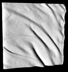
 The drapery surface after filling in the non-fold part. It is viewed at a slightly different angle and lighting direction.")

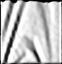
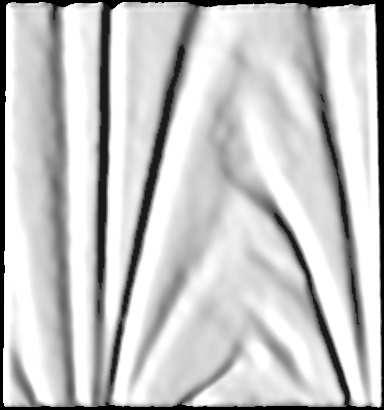
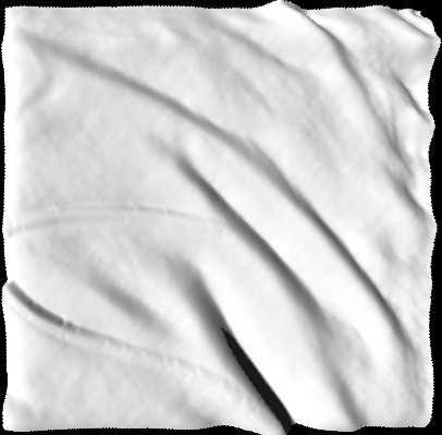
5 5 (a) I (b) G Fig. 2. (c) S fd (d) S (a). A drapery image under approximately parallel light. (b). The sketch graph for the computed folds. (c). The reconstructed surface for the folds. (d) The drapery surface after filling in the non-fold part. It is viewed at a slightly different angle and lighting direction. stant albedo with Lambertian reflectance, (ii) single light source far from the scene, and (iii) orthographic camera projection. These assumptions are approximately observed in the drapery/clothes images in our study due to the uniform color and small relative surface depth compared with distance to the camera, except that some valleys between two deep folds have inter-reflectance and shadows. For such dark areas, we do not apply the SFS equation, but interpolate them by surface smoothness prior between the 3D folds. B. Previous work in shape from shading and cloth representation Shape from shading is a classical ill-posed vision problem studied in Horn s seminar work [15], [16], [18]. Most algorithms in the literature impose smoothness priors for regularization. The state of the art algorithms are given in Zheng and Chellappa [33] and others [20],
6 6 [21], [28], [31], and a survey is given in [32]. These prior models are Markov random field on pixels, which, in our opinion, are rather weak for reconstructing surfaces, and therefore more knowledge about the objects in the scene need to be incorporated for robust computation. This motivates our two-level generative model with dictionary of fold primitives. Our attempt of learning fold primitives is related to two recent work. The first is the socalled shape-from-recognition by Nandy and Ben-Arie [24] and Atick et al [1]. [1] built a probabilistic 3D model for the whole human face in an off-line learning phase, while [24] divided human face into generic parts like nose, lips and eyes and built the 3D prior models of these parts. These models are much better informed than the smoothness priors in SFS and enable them to infer 3D face surface from a single image by fitting a small number of parameters. Their work demonstrates that one can solve SFS better when high level knowledge about the object class is available. The second example is the learning of textons including lightons in Zhu et al [36]. This work learns generic dictionary of surface patches under varying illuminations. In comparison, our fold primitives are focused on drapery and clothes images, and we believe the same method can be extended to other object classes. The two-level model is also closely related to the primal sketch representation in Guo et al [10], [11]. Drapery/cloth representation is also an interesting problem studied in both vision and graphics, as clothes are complex visual patterns with flexible shapes and shading variations. In the graphics literature, clothes are always represented by meshes with a huge number of polygons in geometric based, physical based, and particle based cloth modeling and simulation techniques [17], [4]. Such representation is infeasible for vision purposes. In contrast, artists have long noticed that realistic drapery/clothes can be painted by a few
7 7 types of folds [25]. In the vision literature, methods for detecting folds have been studied in Huggins et al [19] and Haddon and Forsyth [12], [13], mostly using discriminative method. Besides computing the 3D surfaces, the fold representation is also useful for some applications, such as, non-photorealistic human portrait and cartoon sketch, clothed human understanding and tracking. C. Paper Organization The rest of the paper is organized as follows. Section II briefly reviews the formulation of shape from shading and photometric stereo. Section III presents the two-level representation for both 2D cloth images and 3D cloth surfaces. Section IV and Section V discuss the learning and inference algorithms for cloth sketching and reconstruction. Section VI shows the experiments with comparison results. Section VII concludes the paper with a discussion of limitation and future work. II. Problem formulation of shape from shading and photometric stereo This section discusses the formulation of two problems which will be used as components in our generative models and algorithms. (i) Shape from shading for the non-fold part. (ii) Photometric stereo used in constructing 3D cloth surface for learning the fold primitive dictionary. A. Formulation of shape from shading Considering a surface observed under orthographic projection, we define the coordinate system so that its x and y axes span the image plane Λ and z axis coincides with the optical
8 8 axis of the camera. Thus the surface S is expressed as a depth map, S(x, y) = z(x, y), (x, y) Λ. (1) Following the notation of Horn [15], we denote the surface gradients at (x, y) by (p, q) with p(x, y) = S(x, y), q(x, y) = x S(x, y). (2) y The unit normal of the surface is, p n = ( p2 + q 2 + 1, q p2 + q 2 + 1, 1 p2 + q ) (3) For Lambertian surface with constant composite albedo (including strength of illumination and reflectivity of the surface) η, we obtain a reflectance map R under parallel light L = (l 1, l 2, l 3 ), R = η < n, L >= η pl 1 ql 2 + l 3 p2 + q (4) Eqn. 4 is the basic image irradiance equation in SFS. R can be written as either a function R = R(p, q, η, L) or an image R = R(x, y). The light source L is a unit vector, which can be equally represented by the lighting angle (γ, τ) for the slant and tilt. So (l 1, l 2, l 3 ) = (cos τ cos γ, cos τ sin γ, sin τ). In the literature, the composite albedo η and light direction (γ, τ) are three global variables that can be inferred quite reliably without computing (p, q, S). There are two statistical approaches for estimating η and (γ, τ) by Lee and Rosenfeld [21] and Zheng and Chellapa [33]. In this paper, we adopt the method in [33]. The computation of (p, q, S) are based on the computation of η and (γ, τ) in the rest of the paper. Since there are infinite number of surfaces that can produce the same intensity image I, some additional constraints are needed to regularize the problem in the form of energy
9 9 functions. In the literature, one may impose the smoothness energy on the surface S, or alternatively one may put the smoothness energy plus an integrability energy on the gradients (p, q) and derive S from (p, q). The latter is more convenient for computation, and is adopted in this paper. The following is an energy on (p, q) in [8] modified by smoothness weights in [30], E 1 (p, q) = λ int (x,y) Λ (p y q x ) 2 + λ smo (x,y) Λ (w 1 p 2 x + w 2 p 2 y + w 2 q 2 x + w 3 q 2 y). (5) The first term is an integrability term, the second term is an inhomogeneous smoothness term, and λ int and λ smo are parameters balancing the two parts 1. w 1, w 2, and w 3 are the weights used in [30], which are chosen to be inversely proportional to the intensity gradient along the x, diagonal, and y directions respectively. To compute these weights, one normalizes the image intensity to [0, 1], and calculates w 1 (x, y) = (1 I x (x, y) ) 2, w 2 (x, y) = (1 2 2 I x(x, y) + I y (x, y) ) 2, and w 3 (x, y) = (1 I y (x, y) ) 2. The deterministic relation in eqns.(2) is relaxed to a soft energy between S and (p, q), E 2 (S p, q) = (x,y) Λ (S x p) 2 + (S y q) 2. (6) The residue between a radiance image R and input image I is assumed to be Gaussian noise. For shadowed areas (deep and narrow valleys between folds), the image intensities (lower than a threshold δ) no longer follow the Lambertian assumption, and thus they do not contribute to the data energy term below. We denote the shadow pixels by Λ o = {(x, y) : I(x, y) δ}. The third energy term is, E 3 (I p, q, η, L) = (x,y) Λ\Λ o (I(x, y) R(x, y))2 2σ 2. (7) 1 As a side note, the smoothness energy function together with the parameters could be learned from data using a minimax entropy principle as it was done in [35].
10 10 R is a function of p, q, η, L. In summary, the following are the common energy terms for shape-from-shading which will be used in the non-fold area in this paper, E nfd (S, p, q I) = E 1 (p, q) + E 2 (S p, q) + E 3 (I p, q, η, L). (8) As we stated before, the composite albedo η and lighting direction (γ, τ) are estimated in an initial stage. In a Bayesian formulation, energy minimization is equivalent to maximizing a posteriori probability, (S, p, q) = arg max p(i p, q, η, L)p(S p, q)p(p, q). (9) The three probabilities are exponential models with energies E 3 (I p, q, η, L), E 2 (S p, q), and E 1 (p, q) respectively. In general, S, p, q are all unknowns and have to be inferred simultaneously in iterations together with the global variables η and (γ, τ). In practice, people often compute them sequentially for computational efficiency. First we compute the gradient map (p, q) by minimizing E 1 + E 3, and the we construct the surface map S by minimizing E 2. A well-known phenomenon in SFS is the in-out ambiguity [26] that people may experience when we view the shading images. For the drapery image in Fig. 2.(a), our preception may flip between convex and concave for some parts. Such ambiguity could be resolved by the shadows in the deep valley. B. Formulation of photometric stereo For a static surface S and fixed camera, one may obtain multiple images I i under varying lighting directions L i for i = 1, 2,..., m. Then we can acquire the 3D surface S from these
11 11 images. This is the standard photometric stereo technique [27]. We shall use photometric stereo to obtain surface depth for supervised learning of the fold primitives in later section. We write each reflectance image R i in a Λ 1 column vector and n a Λ 3 matrix, then we have a group of linear equations (R 1, R 2,..., R m ) =< ηn, (L 1, L 2,..., L m ) >. (10) One can solve n by minimizing the sum of squared errors n = m (I i (x, y) R i (x, y)) 2. (11) i=1 (x,y) This is solved by singular value decomposition (SVD). For surface with constant reflectance η, it is well known that the SVD solution will have an in-out ambiguity. The in-out ambiguity can be resolved by the observation of shadows. III. Drapery/cloth representation by a two-layer generative model In this section, we introduce the folds, the two-level generative model for both the 2D cloth images and the 3D cloth surfaces, then we formulate the SFS problem in Bayesian framework with this two-level generative model. A. The sketch graph for fold representation The sketch graph G in Fig. 1 is an attribute graph consisting of a number of folds f i, i = 1, 2,..., N fd. Each fold f i is a smooth curve which is divided into a chain of fold primitives. Fig. 3 shows an example of the folds (in curves) and fold primitives (in deformed rectangles). We pool all the fold primitives of G in a set V. V = {π i = (l i, θ geo i, θ pht i, θ prf i, Λ i ) : i = 1, 2,..., N prm }. (12)
12 12 Each fold primitive π i V covers a rectangle domain Λ i Λ. It is usually 15-pixel long and 9-pixel wide and has the following attributes to specify the 3D surface and image intensity within its domain Λ i. 1. A label l i indexing the three types of 3D fold primitive in the dictionary fd (to be introduced next section). 2. The geometric transformation θ geo i including the center location x i, y i, depth z i, tilt ψ i, slant φ i, scale (size) σ i, and deformation (shape) vector δ i. The latter stretches the rectangle to fit seamlessly with adjacent primitives. 3. The photometric attributes θ pht i including the light source (l 1i, l 2i, l 3i ), and surface albedo η i. Here we assume all the fold primitives share the same light source and surface albedo. But this assumption could be relaxed in case of multiple light sources in future study. 4. The surface (depth) of each primitive is represented by the profile (cross-section) perpendicular to the principal axis of the rectangle of the primitive, and therefore is specified by parameters θ prf i. As the surface profile is represented by PCA introduced later, θ prf i a few coefficients for the PCA. 5. The image domain Λ i which is controlled fully by the geometric transforms θ geo i. includes B. Two-layer generative model As Fig. 3.(b) shows, the graph G divides the image lattice into two disjoint parts the fold and non-fold areas, Λ = Λ fd Λ nfd, Λ fd Λ nfd =. (13) Thus both the image and the surface are divided into two parts, I = (I fd, I nfd ), S = (S fd, S nfd ). (14)

13 13 (a) (b) Fig. 3. (a) The graph G with rectangular fold primitives, and (b) the partition of the image domain Λ in the two-level representation of an image shown in second column of Fig. 11 (a). In general, I fd captures the most information and I nfd has only secondary information and can be approximately reconstructed from I fd. Fig. 4 is an example illustrating this observation. Fig. 4.(a) is an image of clothes, (b) is the sketch graph G, and (c) is the reconstructed I fd using shading primitives in sd (to be introduced soon) with attributes in G, and (d) is the reconstructed image after filling-in the non-fold part by simple heat diffusion. The heat diffusion has fixed boundary condition I fd and therefore it does not converge to uniform image. I(x,y,t) t = α( 2 I x I 2 y ), (x, y) Λ nfd, I(x, y, t) = I fd (x, y), (x, y) Λ fd, t 0. (15) As we know, the heat diffusion is a variational equation minimizing a smoothness energy (prior). Thus filling-in the non-fold part with the probabilistic models (formulated in eqn.(9)) should achieve similar visual effects. In the literature, it has long been observed, since Marr s primal sketch concept [23] that edge map plus gradients at edges (sketches here) contains almost sufficient image information
input cloth image. (b) The sketch graph G.")

![A more rigorous mathematical model for integrating the structural (sketch) with textures is referred to the recent primal sketch representation in [10], [11].](/docs-images/86/93796500/images/14-2.jpg "The fold area Λ fd is further decomposed into a number of primitive domains Λ fd = Nprm i=1 Λ i.")
14 14 (a) Input (b)folds graph G (c)i fd (d) Filling result Fig. 4. Fill-in the non-fold part by smooth interpolation through diffusion. This figure demonstrates the observation that the folds contains most information about the image. (a)input cloth image. (b) The sketch graph G. (c) The fold part I fd reconstructed from the shading primitives with G. (d) Reconstructed cloth image by filling in I nfd by heat diffusion equation with I fd being the fixed boundary condition. [9] and this has been used in inpainting methods [6]. A more rigorous mathematical model for integrating the structural (sketch) with textures is referred to the recent primal sketch representation in [10], [11]. The fold area Λ fd is further decomposed into a number of primitive domains Λ fd = Nprm i=1 Λ i. (16) Within each primitive domain Λ i, the surface is generated by the attributes on geometric transforms θ geo and profile parameters θ prf, S i (x, y) = B li (x, y; θ prf i, θ geo i ), (x, y) Λ i, (17) where B li fd is a 3D fold primitive in the dictionary fd (next section) indexed by the type l i. S i yields the gradients (p, q) and generates the radiance image using the photometric attributes θ pht i = (η i, l 1i, l 2i, l 3i ), pl 1i ql 2i + l 3i R i (x, y) = η i p2 + q 2 + 1, (x, y) Λ i. (18)
15 15 In fact, we can rewrite the radiance image in terms of the shading primitive, R i (x, y) = b li (x, y; θ prf i, θ geo i, θ pht i ), (x, y) Λ i, (19) with b li sd being a 2D image base in the shading primitive dictionary sd (next section). The overall radiance image for the fold part is the mosaic of these radiance patches. In short, we have a generative model for R fd on Λ fd with the dictionary being parameters of the generative model. R fd = R(G; ); = ( fd, sd ). (20) Since each domain Λ i often covers over 100 pixels, the above model has much lower dimensions than the pixel-based representation in conventional SFS methods. The generative relation is summarized in the following, G S fd (p fd, q fd ) R fd I fd. Therefore we can write the energy function for the fold part in the following, E fd (G I fd ) = E 4 (I fd G) + E 5 (G). (21) E 4 is a likelihood term, where Θ i = (θ prf i, θ geo i E 4 (I fd G) = N prm i=1 (I(x, y) b li (x, y; Θi))2, (22) 2σ 2 (x,y) Λ i, θ pht i ). E 5 is a prior term on the graph G. As G consists of a number of N fd folds (smooth curves f 1,...f Nfd ), E fd (G) penalizes the complexity K and each fold f i is a Markov chain model whose energy is learned in a supervised way (next section). E 5 (G) = λ 0 K + K E 0 (f i ). (23) i=1
16 16 We denote by E 0 (f i ) the coding length of each fold (see eqn.(28)). So far, we have a generative model for the fold surface S fd and radiance image R fd on Λ fd. The remaining non-fold part has flat surface S nfd and nearly constant radiance R nfd. One could use the traditional shape-from-shading method for the non-fold part conditioning on the fold part. Therefore we have the following objective function, E SFS2 (G, S, p, q I) = E fd (G I fd ) + E nfd (S, p nfd, q nfd I nfd, p fd, q fd ) (24) The second energy is rewritten from eqn. (8). In summary, the overall problem is formulated as, (G, S, p, q) = arg min E SFS2 (G, S, p, q I). (25) In the computational algorithm, we solve the variables in a stepwise manner. We first compute G by minimizing E fd (G I fd ) = E 5 + E 4. Then with G we can derive the gradients (p fd, q fd ) for the fold part, which will be used as boundary conditions in computing the gradients (p nfd, q nfd ) at the non-fold part through minimizing E 1 + E 3. Finally we infer the joint surface S from (p, q) over Λ by minimizing E 2. In the next section, we shall learn the 3D fold primitive dictionary fd, the shading primitive dictionary sd, and the Markov chain energy E fd (G) for the smoothness of folds. IV. Learning the fold primitives and shape This section discusses the supervised learning of the 3D fold primitive dictionary fd and its derived 2D shading primitive dictionary sd, and the Markov chain energy for the fold shape. They are part of the two-level generative model.
 are three of the twenty images for two drapery/cloth surfaces.")


 are three of the twenty images and (d) is the reconstructed surface.")


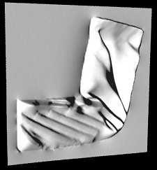
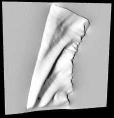
17 17 (a) (b) (c) (d) Fig. 5. (a-c) are three of the twenty images for two drapery/cloth surfaces. (d) is the reconstructed 3D surfaces using photometric stereo. A. Learning 3D fold primitives We use the photometric stereo algorithm [27] to acquire some 3D drapery/cloth surfaces for training. For each of drapery/cloth surface, we take about 20 images under different lighting conditions (nearly parallel light) with a fixed camera. Two examples are shown in Fig. 5 where (a-c) are three of the twenty images and (d) is the reconstructed surface. As we discussed in Section II, the photometric stereo has an in-out ambiguity for uniform reflectance surfaces. Such ambiguity can be resolved with shadow and object boundary information. For example, our perception may flip between concave and convex surfaces for the drapery (Fig.5.(a) and (b) top row). We build an interface program to manually extract fold patches on the 3D surfaces. We draw the fold curves on the ridge (not valleys) and define the width of the fold (or scale) by rectangles whose principal axes are aligned with the ridges (See Fig. 3.(a)). We extract the surface profile at the cross-section perpendicular to the ridge (axis) within the rectangles.

18 18 Examples of surface profile at cross-sections Fig. 6. Three types of fold profiles defined are shown at the top which correspond to the solid, dashed, and dotted lines respectively. The right side shows some typical examples of the surface profile at the cross-sections perpendicular to the folds. We define three types of folds according to their surface profiles as Fig.6 shows. The first type (in solid curves) is the full fold a ridge in frontal view. The other two types (in dashed and dotted curves) are half folds which are either a ridge in side views or the two boundaries of a broad ridge in frontal view. We show the folds on an image not the 3D surface for better view. By analogy to edge detection, the full folds are like bars and half folds are like step edges. The top row in Fig. 6 shows the surface profiles of the three types of folds. These profiles are the cross-section of the surface (from photometric stereo) perpendicular to the folds (one may call them curves, sketches, or strokes) and the right hand panel shows some examples. Note that we only represent the ridges not the valleys for two reasons. (i) The valleys can be constructed from the ridges through surface smoothness assumption. (ii) The valleys often have heavy inter-reflectance and shadows. Their radiances are less regular than the
19 19 ridges in terms of parametric modeling. We tried to introduce a fourth primitive for the shadowed deep valleys, but practically we find that such deep valleys can be reconstructed from two nearby folds. We use principal component analysis (PCA) to represent the surface profiles. Given a number of cross-section profiles for each types of folds, we warp and interpolate to align them to have the same vector length. Then we compute the mean and a small number (3 5) of eigen-vectors of the profiles. So the cross-section profile is represented by a few PCA coefficients denoted by θ prf. Along the fold axis, the surface is assumed to be the same (a sweep function) except that slight smoothness adjustments are needed to fit two adjacent primitives together. Therefore, we have a dictionary of 3D fold primitives. fd = {B l (x, y : θ prf, θ geo ) : θ prf Ω l, θ geo Ω geo, l = 1, 2, 3.}. (26) Each fold primitive B is a 3D surface patch specified by the surface variables θ prf and variables θ geo for geometric transforms and deformations. In fd, Ω l denotes the space of the surface profiles for each type l, and Ω geo denotes the space of geometric transforms. A 2D shading primitive dictionary sd is derived from fd by adding the illumination variables θ pht Ω pht. sd = {b l (x, y : θ prf, θ geo, θ pht ) : θ prf Ω l, θ geo Ω geo, θ pht Ω pht, l = 1, 2, 3.}. (27) Each shading primitive b l is an image patch generated from a surface patch B l under lighting condition θ pht. The shading primitives are similar to the lightons studied in [36]. As we discussed in Section (III), G is an attribute graph and each vertex is a 3D fold primitive that has all the attributes l, θ prf, θ pht, θ geo.

, we model each fold as a third-order Markov chain (trigram).")
 j=3 The conditional probability ensures smooth changes of the following attributes of adjacent primitives. 1.")
20 20 three viewing directions four lighting trajectories Fig. 7. The rendering results for the learned mean fold shape under different viewing directions and lighting conditions. B. Learning shape prior for folds The graph G consists of a number of folds {f i : i = 1, 2,..., N fd } with each fold f i being a smooth attribute curve. Suppose a fold f has N f primitives f = (π 1, π 2,..., π Nf ), we model each fold as a third-order Markov chain (trigram). N f p(f) = p(π 1, π 2 ) p(π j π j 1, π j 2 ). (28) j=3 The conditional probability ensures smooth changes of the following attributes of adjacent primitives. 1. The orientation (tilt ψ and slant φ) in 3D space. 2. The primitives scale (width) σ. 3. The surface profile on θ prf. These probabilities are assumed to be Gaussians whose mean and covariance matrices are learned from the manually drawn folds. Then we can transform the probability p(f) into
21 21 energy functions E 0 in eqn. (23). We do not model the spatial arrangements of the folds, for it leads to a three-level model as Section VII discusses (see Fig. 14). V. Inference Algorithm for the folds and surface The overall computing algorithm has been shown in Fig. 1. In this section, we discuss the algorithm in details. The algorithm proceeds in two phases. In phase I, we run a greedy sketch pursuit algorithm to find all folds in the sketch graph G from the input image. At each step, the algorithm selects one shading primitive from sd by either creating a new fold or growing an existing fold so as to achieve the maximum reduction of the energy function following the formulation of the previous section. The energy function favors a primitive which has good fit to the dictionary and is aligned well with an existing primitive. This procedure is similar to the matching pursuit algorithm [22] in signal decomposition with wavelet dictionary, as well as the sketch pursuit in the primal sketch work [10], [11]. To expedite the pursuit procedure, we use a discriminative method [12] to detect the fold candidates in a bottom-up step. These fold candidates are proposed to the sketch pursuit algorithm which sorts the candidate primitives according to some weights and selects the primitives sequentially using a top-down generative model. This is much more effective than simply trying all shading primitives at all locations, scales and orientations in the dictionary fd. Therefore the algorithm bears resemblance to the datadriven Markov chain Monte Carlo methods [34], [29] except that our method is a greedy one for simplicity of the fold shape. In phase I, we also compute the 3D folds and surface S fd by fitting the shading primitives to the 3D fold dictionary with the estimated composite albedo η and lighting direction (τ, γ).
 for the non-fold areas using the existing SFS method and recover the surface S nfd with the fold surface S fd as boundary condition in a precess of")


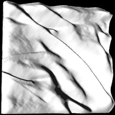
22 22 (a) (b) (c) Fig. 8. (a) Input image. (b) Ridge detection result. (c) Proposed positions of folds. In phase II, we compute the gradient map (p, q) for the non-fold areas using the existing SFS method and recover the surface S nfd with the fold surface S fd as boundary condition in a precess of minimizing a joint energy function. A. Bottom-up detection of fold candidates by discriminative methods An important feature for detecting folds is the intensity profile for the cross sections of the folds. It is ineffective to examine all possible cross sections at all possible locations, orientations, and scales. Therefore we adopt the idea of detection by a cascade of features in the recent pattern recognition literature and thus detect the fold candidates in two steps as Fig. 8 shows. In the first step, we run a ridge detection method [14] to locate the possible locations of the ridges and estimate their local orientations. A similar method was also used in [19]. Fig. 8.(b) is an example of the ridge detection results. Then the intensity profiles at the strong ridge locations are extracted perpendicular to the ridge direction. In the second step, we train a support vector machine [12] for binary classification fold vs non-fold by supervised learning using the images we collected in the photometric
23 23 stereo stage. Then we test the intensity profiles at various scales (widths) for the locations and orientations extracted in the ridge detection step. Fig. 8.(c) shows an example of the detected folds in the bottom-up step. As we can see in Fig. 8.(c) that the bottom-up methods detect the salient locations which will largely narrow the top-down search scope. There are two problems with the bottom-up detection: (i) disconnected segments which have to be removed or connected, and (ii) redundant points along the folds which have to be suppressed. At each detected fold position, we do parameter fitting using the fold dictionary and get one candidate fold primitive. We denote the set of all obtained candidate fold primitives as Φ = {(π o i, ω i ) : i = 1, 2,..., N can }. (29) Each π o i is a candidate fold primitive having its own label, geometric transformation and surface profile. The associated ω i is a weight for measuring the prominence of the fold candidate which will be computed from the Bayesian probability formulation as discussed next. B. Computing folds by sketch pursuit with the generative model Our goal in this section is to infer the folds in the sketch graph G following the generative model in Section (III). To simplify the computation, we make two assumptions which will be released in the next step. (i) We assume the non-fold area is a flat surface S nfd and thus has a constant radiance image R nfd = Rnfd o. S nfd will be inferred in the next subsection, (ii) We assume the fold surface S fd is deterministically decided by the attribute graph G, and S fd will be adjusted in the next subsection to achieve global consistence.
24 24 Therefore, the Bayesian formulation in eqn.(25) is simplified as G = arg max p(i G)p(G) = arg min L(I G) + L(G) (30) L(G) and L(I G) are the energy for the prior terms and likelihood respectively defined in Section (III). Here we use the notation L to replace E due to the new composition of energy terms. L(G) = λ o K + L(I G) = N prm i=1 K E o (f i ) i=1 (I(x, y) b li (x, y; Θ i))2 (I(x, y) Ro nfd (x, y))2. 2σ 2 2σ 2 (x,y) Λ i \Λ o I(x,y) Λ nfd \Λ o We initialize G = with the number of folds and primitives being zero (K = N prm = 0) and Λ nfd = Λ. Then the algorithm computes G sequentially by adding one primitive in the candidate set π + Φ at a time. π + may be a seed for starting a new fold or it may grow an existing fold f i. Therefore we have G + = G {π + }. The primitive π + is selected from the candidate set Φ so that it has the maximum weight, π + = arg max π Φ {ω(π) = L(I G) L(I G +) + L(G) L(G + )} (31) The image likelihood term favors a primitive that has a better fit to a domain Λ i against a constant image R o nfd as the background (null hypothesis). The prior term favors a primitive that has a good fit in position, scale, and orientation to existing fold according to the fold prior in eqn (28). The seed primitive that starts a new fold will receive an extra penalty λ o in the prior term. The weight ω(π) for each π Φ is initialized by the difference of the likelihood term plus a prior penalty for π being a seed for new fold. That is, ω(π i ) = λ o + (x,y) Λ i \Λ o { (I(x, y) Ro nfd (x, y))2 2σ 2 (I(x, y) b l i (x, y; Θ i )) 2 2σ 2 }. (32)

 only sums over Λ i \ Λ +.")

25 25 (a) iteration 53 (b) iteration 106 (c) iteration 159 (d) iteration 212 (e) iteration 265 (f) iteration 317 Fig. 9. The state of sketch graph G at iteration 53, 106, 159, 212, 265, 317 on the cloth image shown in Figure 8. Each time after a new primitive π + (with domain Λ + ) is added, the weights of other primitive candidates π i Φ will remain unchanged unless in the following two cases. Case I: π i overlaps with π +. As the pixels in Λ i Λ + has been explained by π +, then for π i the likelihood term in eqn. (32) only sums over Λ i \ Λ +. Therefore the weight ω(π i ) usually is reduced after adding π + to G. Case II: A few neighboring candidate primitives which fit well with π + and can be considered the next growing spot from π +. For such neighbors π i, the prior term penalty λ o is then replaced by the less costly smoothness energy in the Markov chain model E o (f) in eqn. (28). Therefore the weight ω(π i ) is increased after adding π + to G The candidates with changed weights are sorted according to the updated weights, and
26 26 8 x Primitive Weight Iteration Fig. 10. The plot of the weight ω(π + ) (vertical axis) for the newly added primitive π + at each iteration (horizontal axis). the procedure stops when the heaviest candidate has weight less than a threshold ω(π + ) δ o (δ o = 0 in our experiment). Figure 9 shows an experiment for the sketch pursuit procedure at 53, 106, 159, 212, 265, and 317 iterations respectively. The plot of the weight ω(π + ) at each iteration is shown in Figure 10. To summarize, we have the following algorithm for pursuing the sketch graph G. The algorithm for sketch pursuit process 1. Bottom-up phase I: ridge detection for fold location and orientation. 2. Bottom-up phase II: SVM classification of fold primitives to obtain a candidate set Φ. 3. Initialize G, Λ nfd = Λ, and R nfd = Rnfd o. 4. Add a new primitive to G. G G {π + } with highest weight ω(π + ) = arg max{ω(π) : π Φ}. 5. Update the weights ω(π) for the neighboring primitives π Φ of π Re-sort the candidate primitives according to their weights in decreasing order. 7. Repeat 4-6 until ω(π + ) δ o.
27 27 After computing G, we obtain the fold primitives from the shading primitives by fitting the radiance equation with the estimated composite albedo η and lighting direction (γ, τ). Therefore we obtain an estimate for the fold surface Ŝfd. One problem with the estimated depth map Ŝfd is that the depth of each primitive is estimated locally in the domain Λ i. Thus it has one degree of freedom for its absolute depth. As a result, the relative depth between any two folds f i, f j are undecided. The relative depth must be decided together with the non-fold areas in solving the whole surface. C. Infer the non-fold surface and refine the fold surface Given the estimated fold surface Ŝfd, we estimate the gradient map (p fd, q fd ) on Λ fd which is not affected by the undecided depth constant at each fold primitive. In the next step, we infer the gradient maps (p nfd, q nfd ) for the non-fold surface Λ nfd using (p fd, q fd ) on Λ fd as boundary condition. Thus we rewrite the energy in eqn.5 in the following, E 1 (p nfd, q nfd p fd, q fd ) = λ int (p y q x ) 2 +λ smo (w 1 p 2 x+w 2 p 2 y+w 2 qx+w 2 3 qy). 2 (33) (x,y) Λ nfd (x,y) Λ nfd We take a gradient method in [8] for minimizing the energy with respect to (p nfd, q nfd ). At each iteration, we compute the gradient E 1 (p nfd, q nfd ) and choose a discrete stepsize d so that the energy is minimized along the gradient direction. The procedure stops until the decrease of energy is less than a threshold proportion to the number of Λ nfd. Now we have the gradient map (p, q) for the whole image domain Λ, and we compute the surface S = (S fd, S nfd ) by minimizing the following energy term rewritten from eqn.6, E 2 (S p, q) = (S x p) 2 + (S y q) 2. (34) (x,y) Λ We solve the above minimization problem using the just discussed gradient method in [8]. This will be our final result for the surface.
28 28 To conclude this section, we list the steps of the overall algorithm. The algorithm seeks for greedy steps for estimating the variables η, (γ, τ), G, S fd, (p nfd, q nfd ), S nfd sequentially by minimizing some energy terms. The overall algorithm for SFS with the two-level generative model 1. Estimate the global variables: the composite albedo η and lighting direction (γ, τ). 2. Compute the sketch graph G by the fold pursuit process. 3. Initialize the fold surface Ŝfd by fitting the radiance equations. 4. Compute the gradient map (p fd, q fd ) for the fold part. 5. Compute the gradient map (p nfd, q nfd ) for the non-fold part conditioned on (p fd, q fd ). 6. Estimate the cloth surface S = (S fd, S nfd ) jointly from (p, q). It is valuable in theory to estimate the variable in iterations for more accurate result which maximizes the Bayesian posterior probability jointly. For example, adjusting the estimation of η, γ, τ or G after computing S. In practice, we find these greedy steps often obtain satisfactory results, and therefore do not pursue the maximization of the joint posterior probability. VI. Experiments We test our whole algorithm on a number of images. Figure 11 shows the results for three images of drapery hung on wall and a cloth image (last column) on some people. Figure 12 shows four cloth images on people. The lighting direction and surface albedos for all the testing cloth are estimated by the method in [33]. In the experimental results, the first row are input images, the second row are the sketches of folds in the input images and their domain, the third row are the syntheses for I fd based on the generative sketch model for the fold areas, the fourth row are the 3D reconstruction
 (c)")
 Fig.")


.")


29 29 (a) (b) (c) (d) (e) (f) Fig. 11. (a). Input cloth image. (b). 2d folds and their image domains. (c). Synthesis for 2D fold sketches I fd. (d). 3D reconstruction S fd for fold areas. (e-f). Final reconstructed surface S in novel views.
 (c)")
 Fig.")


.")


30 30 (a) (b) (c) (d) (e) (f) Fig. 12. (a). Input cloth image. (b). 2d folds and their image domains. (c). Synthesis for 2D fold sketches I fd. (d). 3D reconstruction S fd for fold areas. (e-f). Final reconstructed surface S in novel views.
. Cloth reconstruction results by approach in (Lee and Kou, 1993).")


31 31 (a) (b) (c) Fig. 13. (a). Input cloth images. (b). Cloth reconstruction results by approach in (Zheng and Chellappa, 1991). (c). Cloth reconstruction results by approach in (Lee and Kou, 1993). results S fd for the fold areas, while fifth and sixth rows are the final reconstruction results of the whole cloth surface S shown in two novel views. In these results, the folds in row (d) have captured most of the perceptually salient information in the input images, and they can reconstruct the surface without too much skewing effects. It makes sense to compute them before the non-fold part. We observe that the SFS for the non-fold parts indeed provides useful information for the 3D positions of the folds. For comparison with the state-of-art-art SFS algorithms, we run two minimization approaches on the same testing images above, as the minimization approaches are more robust and accurate even though much slower than other approaches. The first approach is from [33], while the second one is from [20]. The results for these two approaches are shown in second and third rows respectively in Figure 13. The main problems with these methods
32 32 are: (i) the global surface shape could be skewed (see row (c)) due to the accumulated effect of computing S from the gradient map (p, q) through integration over pixels; and (ii) the relative depth of the folds are not computed reliably. This latter problem is overcome in our method due to the use of fold dictionary. VII. Discussion and future Work The two-level generative model is an attempt to incorporate visual knowledge representation for solving the traditional ill-posed vision problems. The current representation is still limited and shall be extended in the following directions. 1. One may infer a third level generative representation that will explain the spatial relation of the folds. As Fig. 14 shows, the folds are not independently distributed, but are radiated from some hidden structures which artists called hubs [25]. These hubs are shown in dashed ellipses for protruding parts or grip points such as the shoulder, or curves for boundaries such as a waist belt. A fold must start or end with one of these hubs. Physically, these hubs are the stretching points or lines that create the cloth folds. 2. We should learn a richer set of surface and shading primitives for more object classes. One extreme will be the human face model in shape-from-recognition [1], [24], and the other related work is the study of textons and lightons in [36]. With a richer dictionary, we expect that SFS could work for various locations in an image with different types of object primitives even without assuming global parallel lighting conditions. Acknowledgements This work was supported in part by National Science Foundation grants IIS and IIS We thank Jinhui Li for collecting some of the drapery and cloth images used
 and (d) are the folds with additional dashed ellipses and lines which represent a third hidden level for stress areas and boundaries that cause the folds for the image in (a) and (c).")
![They are the sources and sinks for the folds. This calls for a three-level generative model. in photometric stereo and shading, and thank Dr. Yingnian Wu for stimulating discussions. References [1] J.](/docs-images/86/93796500/images/33-1.jpg "J. Atick, P.A. Griffin and A.N. Redlich Statistical Approach to Shape from Shading: Reconstruction of 3-Dimensional Face Surfaces from Single 2-Dimensional Images, Neural Computation, vol. 8, no.")
33 33 (a) (b) (c) (d) Fig. 14. (a) and (c) are respectively a drapery and a cloth image image. (b) and (d) are the folds with additional dashed ellipses and lines which represent a third hidden level for stress areas and boundaries that cause the folds for the image in (a) and (c). They are the sources and sinks for the folds. This calls for a three-level generative model. in photometric stereo and shading, and thank Dr. Yingnian Wu for stimulating discussions. References [1] J.J. Atick, P.A. Griffin and A.N. Redlich Statistical Approach to Shape from Shading: Reconstruction of 3-Dimensional Face Surfaces from Single 2-Dimensional Images, Neural Computation, vol. 8, no. 6, pp , August [2] A.B. Barbu and S.C. Zhu, Incorporating Visual Knowledge Representation in Stereo Reconstruction, Submitted to ICCV, [3] P.N. Belhumeur and D. Kriegman, What Is the Set of Images of an Object Under All Possible Illumination Conditions?, Int l J. Computer Vision, vol. 28, no. 33, pp , [4] K. Bhat, C. D. Twigg, J. K. Hodgins, P.K. Khosla, Z. Popvic, and S.M. Seitz, Estimating Cloth Simulation Parameters from Video, Proc. Symposium on Computer Animation, pp , [5] V. Blanz and T. Vetter, A Morphable Model for the Synthesis of 3D Faces, Computer Graphics Proceedings SIGGRAPH, pp , [6] T. Chan and J. Shen, Local inpainting model and TV inpainting, SIAM J. of Applied Math., 62:3, , [7] C. Cortes and V. Vapnik, Support Vector Networks, Machine Learning, vol. 20, no. 3, pp ,
34 [8] A. Crouzil, X. Descombes and J.-D Durou, A Multiresolution Approach for Shape From Shading Coupling Deterministic and Stochastic Optimization, IEEE Trans. Pattern Analysis and Machine Intelligence, vol. 25, no. 11, pp , Nov [9] J. H. Elder, Are edges incomplete?, Int l, J. of Computer Vision, 34(2/3), , [10] C.E. Guo, S.C. Zhu and Y.N. Wu, Towards a Mathematical Theory of Primal Sketch and Sketchability, Proc. Int l Conf. Computer Vision, pp , [11] C.E. Guo, S.C. Zhu and Y.N. Wu, Primal Sketch: Integrating Texture and Structure, Preprint No. 416, Department of Statistics, UCLA, [12] J. Haddon and D. Forsyth, Shading Primitives: Finding Folds and Shallow Grooves, Proc. Int l Conf. on Computer Vision, pp , [13] J. Haddon and D. Forsyth, Shape Representations From Shading Primitives, Proc. European Conf. on Computer Vision, pp , [14] R. Haralick Ridges and Valleys on Digital Images, Computer Vision, Graphics, and Image Processing, vol. 22, no. 10, pp , Apr [15] B.K.P. Horn and M.J. Brooks Shape from Shading, MIT Press, [16] B.K.P. Horn, Height and Gradient From Shading, Int l J. Computer Vision, vol. 5, no. 1, pp , [17] D.H. House and D.E. Breen, Cloth Modeling and Animation, A.K. Peters, Ltd., [18] K. Ikeuchi, and B.K.P. Horn, Numerical Shape From Shading and Occluding Boundaries, Artificial Intelligence, vol. 17, pp , [19] P.S. Huggins, H.F. Chen, P.N. Belhumeur, and S.W. Zucker, Finding Folds: On the Appearance and Identification of Occlusion, Proc. IEEE Conf. Computer Vision and Pattern Recognition, pp , [20] K.M. Lee and C.C.J. Kuo, Shape from Shading with a Linear Triangular Element Surface Model, IEEE Trans. Pattern Analysis and Machine Intelligence, vol. 15, no. 8, pp , August [21] C.H. Lee and A. Rosenfeld, Improved methods of estimating shape from shading using the light source coordinate system, Shape from Shading, MIT Press, pp , 1989.
A Survey of Light Source Detection Methods
 A Survey of Light Source Detection Methods Nathan Funk University of Alberta Mini-Project for CMPUT 603 November 30, 2003 Abstract This paper provides an overview of the most prominent techniques for light
Bottom-Up/Top-Down Image Parsing with Attribute Grammar
 1 Bottom-Up/Top-Down Image Parsing with Attribute Grammar Feng Han and Song-Chun Zhu Departments of Computer Science and Statistics University of California, Los Angeles, Los Angeles, CA 90095 {hanf, sczhu}@stat.ucla.edu.
Comment on Numerical shape from shading and occluding boundaries
 Artificial Intelligence 59 (1993) 89-94 Elsevier 89 ARTINT 1001 Comment on Numerical shape from shading and occluding boundaries K. Ikeuchi School of Compurer Science. Carnegie Mellon dniversity. Pirrsburgh.
CHAPTER 6 PERCEPTUAL ORGANIZATION BASED ON TEMPORAL DYNAMICS
 CHAPTER 6 PERCEPTUAL ORGANIZATION BASED ON TEMPORAL DYNAMICS This chapter presents a computational model for perceptual organization. A figure-ground segregation network is proposed based on a novel boundary
Illumination-Robust Face Recognition based on Gabor Feature Face Intrinsic Identity PCA Model
 Illumination-Robust Face Recognition based on Gabor Feature Face Intrinsic Identity PCA Model TAE IN SEOL*, SUN-TAE CHUNG*, SUNHO KI**, SEONGWON CHO**, YUN-KWANG HONG*** *School of Electronic Engineering
Face Re-Lighting from a Single Image under Harsh Lighting Conditions
 Face Re-Lighting from a Single Image under Harsh Lighting Conditions Yang Wang 1, Zicheng Liu 2, Gang Hua 3, Zhen Wen 4, Zhengyou Zhang 2, Dimitris Samaras 5 1 The Robotics Institute, Carnegie Mellon University,
Visual Learning with Explicit and Implicit Manifolds
 Visual Learning with Explicit and Implicit Manifolds --- A Mathematical Model of, Texton, and Primal Sketch Song-Chun Zhu Departments of Statistics and Computer Science University of California, Los Angeles
Bottom-up/Top-Down Image Parsing by Attribute Graph Grammar
 Bottom-up/Top-Down Image Parsing by ttribute Graph Grammar Feng Han and Song-Chun Zhu Departments of Computer Science and Statistics University of California, Los ngeles Los ngeles, C 90095 hanf@cs.ucla.edu,
COMP 558 lecture 16 Nov. 8, 2010
 Shading The term shading typically refers to variations in irradiance along a smooth Lambertian surface. Recall that if a surface point is illuminated by parallel light source from direction l, then the
Reconstruction of Discrete Surfaces from Shading Images by Propagation of Geometric Features
 Reconstruction of Discrete Surfaces from Shading Images by Propagation of Geometric Features Achille Braquelaire and Bertrand Kerautret LaBRI, Laboratoire Bordelais de Recherche en Informatique UMR 58,
Re-rendering from a Dense/Sparse Set of Images
 Re-rendering from a Dense/Sparse Set of Images Ko Nishino Institute of Industrial Science The Univ. of Tokyo (Japan Science and Technology) kon@cvl.iis.u-tokyo.ac.jp Virtual/Augmented/Mixed Reality Three
Face Tracking. Synonyms. Definition. Main Body Text. Amit K. Roy-Chowdhury and Yilei Xu. Facial Motion Estimation
 Face Tracking Amit K. Roy-Chowdhury and Yilei Xu Department of Electrical Engineering, University of California, Riverside, CA 92521, USA {amitrc,yxu}@ee.ucr.edu Synonyms Facial Motion Estimation Definition
Object Recognition Using Pictorial Structures. Daniel Huttenlocher Computer Science Department. In This Talk. Object recognition in computer vision
 Object Recognition Using Pictorial Structures Daniel Huttenlocher Computer Science Department Joint work with Pedro Felzenszwalb, MIT AI Lab In This Talk Object recognition in computer vision Brief definition
Shweta Gandhi, Dr.D.M.Yadav JSPM S Bhivarabai sawant Institute of technology & research Electronics and telecom.dept, Wagholi, Pune
 Face sketch photo synthesis Shweta Gandhi, Dr.D.M.Yadav JSPM S Bhivarabai sawant Institute of technology & research Electronics and telecom.dept, Wagholi, Pune Abstract Face sketch to photo synthesis has
Photometric Stereo. Lighting and Photometric Stereo. Computer Vision I. Last lecture in a nutshell BRDF. CSE252A Lecture 7
 Lighting and Photometric Stereo Photometric Stereo HW will be on web later today CSE5A Lecture 7 Radiometry of thin lenses δa Last lecture in a nutshell δa δa'cosα δacos β δω = = ( z' / cosα ) ( z / cosα
What is Computer Vision?
 Perceptual Grouping in Computer Vision Gérard Medioni University of Southern California What is Computer Vision? Computer Vision Attempt to emulate Human Visual System Perceive visual stimuli with cameras
MULTIRESOLUTION SHAPE FROM SHADING*
 MULTIRESOLUTION SHAPE FROM SHADING* Gad Ron Shmuel Peleg Dept. of Computer Science The Hebrew University of Jerusalem 91904 Jerusalem, Israel Abstract Multiresolution approaches are often used in computer
Bottom-up/Top-Down Image Parsing by Attribute Graph Grammar
 Bottom-up/Top-Down Image Parsing by ttribute Graph Grammar Paper No.: 1238 bstract In this paper, we present an attribute graph grammar for image parsing on scenes with man-made objects, such as buildings,
Video Alignment. Literature Survey. Spring 2005 Prof. Brian Evans Multidimensional Digital Signal Processing Project The University of Texas at Austin
 Literature Survey Spring 2005 Prof. Brian Evans Multidimensional Digital Signal Processing Project The University of Texas at Austin Omer Shakil Abstract This literature survey compares various methods
Robotics Programming Laboratory
 Chair of Software Engineering Robotics Programming Laboratory Bertrand Meyer Jiwon Shin Lecture 8: Robot Perception Perception http://pascallin.ecs.soton.ac.uk/challenges/voc/databases.html#caltech car
A Shape from Shading Approach for the Reconstruction of Polyhedral Objects using Genetic Algorithm
 A Shape from Shading Approach for the Reconstruction of Polyhedral Objects using Genetic Algorithm MANOJ KUMAR RAMA BHARGAVA R. BALASUBRAMANIAN Indian Institute of Technology Roorkee, Roorkee P.O. Box
Segmentation and Tracking of Partial Planar Templates
 Segmentation and Tracking of Partial Planar Templates Abdelsalam Masoud William Hoff Colorado School of Mines Colorado School of Mines Golden, CO 800 Golden, CO 800 amasoud@mines.edu whoff@mines.edu Abstract
Optimal Grouping of Line Segments into Convex Sets 1
 Optimal Grouping of Line Segments into Convex Sets 1 B. Parvin and S. Viswanathan Imaging and Distributed Computing Group Information and Computing Sciences Division Lawrence Berkeley National Laboratory,
Probabilistic Facial Feature Extraction Using Joint Distribution of Location and Texture Information
 Probabilistic Facial Feature Extraction Using Joint Distribution of Location and Texture Information Mustafa Berkay Yilmaz, Hakan Erdogan, Mustafa Unel Sabanci University, Faculty of Engineering and Natural
General Principles of 3D Image Analysis
 General Principles of 3D Image Analysis high-level interpretations objects scene elements Extraction of 3D information from an image (sequence) is important for - vision in general (= scene reconstruction)
Primal Sketch: Integrating Texture and Structure
 Primal Sketch: Integrating Texture and Structure Cheng-en Guo, Song-Chun Zhu, and Ying Nian Wu Departments of Statistics and Computer Science University of California, Los Angeles Los Angeles, CA 90095
A Hierarchical Compositional System for Rapid Object Detection
 A Hierarchical Compositional System for Rapid Object Detection Long Zhu and Alan Yuille Department of Statistics University of California at Los Angeles Los Angeles, CA 90095 {lzhu,yuille}@stat.ucla.edu
Computational Photography and Video: Intrinsic Images. Prof. Marc Pollefeys Dr. Gabriel Brostow
 Computational Photography and Video: Intrinsic Images Prof. Marc Pollefeys Dr. Gabriel Brostow Last Week Schedule Computational Photography and Video Exercises 18 Feb Introduction to Computational Photography
Face Recognition At-a-Distance Based on Sparse-Stereo Reconstruction
 Face Recognition At-a-Distance Based on Sparse-Stereo Reconstruction Ham Rara, Shireen Elhabian, Asem Ali University of Louisville Louisville, KY {hmrara01,syelha01,amali003}@louisville.edu Mike Miller,
Chapter 7. Conclusions and Future Work
 Chapter 7 Conclusions and Future Work In this dissertation, we have presented a new way of analyzing a basic building block in computer graphics rendering algorithms the computational interaction between
Structured Light II. Thanks to Ronen Gvili, Szymon Rusinkiewicz and Maks Ovsjanikov
 Structured Light II Johannes Köhler Johannes.koehler@dfki.de Thanks to Ronen Gvili, Szymon Rusinkiewicz and Maks Ovsjanikov Introduction Previous lecture: Structured Light I Active Scanning Camera/emitter
Correcting User Guided Image Segmentation
 Correcting User Guided Image Segmentation Garrett Bernstein (gsb29) Karen Ho (ksh33) Advanced Machine Learning: CS 6780 Abstract We tackle the problem of segmenting an image into planes given user input.
Estimating Human Pose in Images. Navraj Singh December 11, 2009
 Estimating Human Pose in Images Navraj Singh December 11, 2009 Introduction This project attempts to improve the performance of an existing method of estimating the pose of humans in still images. Tasks
Statistical image models
 Chapter 4 Statistical image models 4. Introduction 4.. Visual worlds Figure 4. shows images that belong to different visual worlds. The first world (fig. 4..a) is the world of white noise. It is the world
Photometric stereo. Recovering the surface f(x,y) Three Source Photometric stereo: Step1. Reflectance Map of Lambertian Surface
 Three Source Photometric stereo: Step1. Reflectance Map of Lambertian Surface") Photometric stereo Illumination Cones and Uncalibrated Photometric Stereo Single viewpoint, multiple images under different lighting. 1. Arbitrary known BRDF, known lighting 2. Lambertian BRDF, known lighting
Photometric stereo Illumination Cones and Uncalibrated Photometric Stereo Single viewpoint, multiple images under different lighting. 1. Arbitrary known BRDF, known lighting 2. Lambertian BRDF, known lighting
A Generative Model of Human Hair for Hair Sketching
 A Generative Model of Human Hair for Hair Sketching Hong Chen and Song Chun Zhu Departments of Statistics and Computer Science University of California, Los Angeles {hchen,sczhu}@stat.ucla.edu Abstract
Lambertian model of reflectance I: shape from shading and photometric stereo. Ronen Basri Weizmann Institute of Science
 Lambertian model of reflectance I: shape from shading and photometric stereo Ronen Basri Weizmann Institute of Science Variations due to lighting (and pose) Relief Dumitru Verdianu Flying Pregnant Woman
Edge and local feature detection - 2. Importance of edge detection in computer vision
 Edge and local feature detection Gradient based edge detection Edge detection by function fitting Second derivative edge detectors Edge linking and the construction of the chain graph Edge and local feature
Last week. Multi-Frame Structure from Motion: Multi-View Stereo. Unknown camera viewpoints
 Last week Multi-Frame Structure from Motion: Multi-View Stereo Unknown camera viewpoints Last week PCA Today Recognition Today Recognition Recognition problems What is it? Object detection Who is it? Recognizing
Human Upper Body Pose Estimation in Static Images
 1. Research Team Human Upper Body Pose Estimation in Static Images Project Leader: Graduate Students: Prof. Isaac Cohen, Computer Science Mun Wai Lee 2. Statement of Project Goals This goal of this project
Applying Synthetic Images to Learning Grasping Orientation from Single Monocular Images
 Applying Synthetic Images to Learning Grasping Orientation from Single Monocular Images 1 Introduction - Steve Chuang and Eric Shan - Determining object orientation in images is a well-established topic
Image Segmentation Using Iterated Graph Cuts Based on Multi-scale Smoothing
 Image Segmentation Using Iterated Graph Cuts Based on Multi-scale Smoothing Tomoyuki Nagahashi 1, Hironobu Fujiyoshi 1, and Takeo Kanade 2 1 Dept. of Computer Science, Chubu University. Matsumoto 1200,
COMPUTER AND ROBOT VISION
 VOLUME COMPUTER AND ROBOT VISION Robert M. Haralick University of Washington Linda G. Shapiro University of Washington T V ADDISON-WESLEY PUBLISHING COMPANY Reading, Massachusetts Menlo Park, California
Image Processing 1 (IP1) Bildverarbeitung 1
 Bildverarbeitung 1") MIN-Fakultät Fachbereich Informatik Arbeitsbereich SAV/BV (KOGS) Image Processing 1 (IP1) Bildverarbeitung 1 Lecture 20: Shape from Shading Winter Semester 2015/16 Slides: Prof. Bernd Neumann Slightly
MIN-Fakultät Fachbereich Informatik Arbeitsbereich SAV/BV (KOGS) Image Processing 1 (IP1) Bildverarbeitung 1 Lecture 20: Shape from Shading Winter Semester 2015/16 Slides: Prof. Bernd Neumann Slightly
Learning to Perceive Transparency from the Statistics of Natural Scenes
 Learning to Perceive Transparency from the Statistics of Natural Scenes Anat Levin Assaf Zomet Yair Weiss School of Computer Science and Engineering The Hebrew University of Jerusalem 9194 Jerusalem, Israel
Other approaches to obtaining 3D structure
 Other approaches to obtaining 3D structure Active stereo with structured light Project structured light patterns onto the object simplifies the correspondence problem Allows us to use only one camera camera
3D Active Appearance Model for Aligning Faces in 2D Images
 3D Active Appearance Model for Aligning Faces in 2D Images Chun-Wei Chen and Chieh-Chih Wang Abstract Perceiving human faces is one of the most important functions for human robot interaction. The active
Mesh segmentation. Florent Lafarge Inria Sophia Antipolis - Mediterranee
 Mesh segmentation Florent Lafarge Inria Sophia Antipolis - Mediterranee Outline What is mesh segmentation? M = {V,E,F} is a mesh S is either V, E or F (usually F) A Segmentation is a set of sub-meshes
Self Lane Assignment Using Smart Mobile Camera For Intelligent GPS Navigation and Traffic Interpretation
 For Intelligent GPS Navigation and Traffic Interpretation Tianshi Gao Stanford University tianshig@stanford.edu 1. Introduction Imagine that you are driving on the highway at 70 mph and trying to figure
Pattern Recognition. Kjell Elenius. Speech, Music and Hearing KTH. March 29, 2007 Speech recognition
 Pattern Recognition Kjell Elenius Speech, Music and Hearing KTH March 29, 2007 Speech recognition 2007 1 Ch 4. Pattern Recognition 1(3) Bayes Decision Theory Minimum-Error-Rate Decision Rules Discriminant
Motion Estimation. There are three main types (or applications) of motion estimation:
 of motion estimation:") Members: D91922016 朱威達 R93922010 林聖凱 R93922044 謝俊瑋 Motion Estimation There are three main types (or applications) of motion estimation: Parametric motion (image alignment) The main idea of parametric motion
Members: D91922016 朱威達 R93922010 林聖凱 R93922044 謝俊瑋 Motion Estimation There are three main types (or applications) of motion estimation: Parametric motion (image alignment) The main idea of parametric motion
Convexization in Markov Chain Monte Carlo
 in Markov Chain Monte Carlo 1 IBM T. J. Watson Yorktown Heights, NY 2 Department of Aerospace Engineering Technion, Israel August 23, 2011 Problem Statement MCMC processes in general are governed by non
Factorization Method Using Interpolated Feature Tracking via Projective Geometry
 Factorization Method Using Interpolated Feature Tracking via Projective Geometry Hideo Saito, Shigeharu Kamijima Department of Information and Computer Science, Keio University Yokohama-City, 223-8522,
Texture Modeling using MRF and Parameters Estimation
 Texture Modeling using MRF and Parameters Estimation Ms. H. P. Lone 1, Prof. G. R. Gidveer 2 1 Postgraduate Student E & TC Department MGM J.N.E.C,Aurangabad 2 Professor E & TC Department MGM J.N.E.C,Aurangabad
EE795: Computer Vision and Intelligent Systems
 EE795: Computer Vision and Intelligent Systems Spring 2012 TTh 17:30-18:45 FDH 204 Lecture 14 130307 http://www.ee.unlv.edu/~b1morris/ecg795/ 2 Outline Review Stereo Dense Motion Estimation Translational
Epitomic Analysis of Human Motion
 Epitomic Analysis of Human Motion Wooyoung Kim James M. Rehg Department of Computer Science Georgia Institute of Technology Atlanta, GA 30332 {wooyoung, rehg}@cc.gatech.edu Abstract Epitomic analysis is
Improving Latent Fingerprint Matching Performance by Orientation Field Estimation using Localized Dictionaries
 Available Online at www.ijcsmc.com International Journal of Computer Science and Mobile Computing A Monthly Journal of Computer Science and Information Technology IJCSMC, Vol. 3, Issue. 11, November 2014,
Robust Model-Free Tracking of Non-Rigid Shape. Abstract
 Robust Model-Free Tracking of Non-Rigid Shape Lorenzo Torresani Stanford University ltorresa@cs.stanford.edu Christoph Bregler New York University chris.bregler@nyu.edu New York University CS TR2003-840
Three-Dimensional Computer Vision
 \bshiaki Shirai Three-Dimensional Computer Vision With 313 Figures ' Springer-Verlag Berlin Heidelberg New York London Paris Tokyo Table of Contents 1 Introduction 1 1.1 Three-Dimensional Computer Vision
CHAPTER 9. Classification Scheme Using Modified Photometric. Stereo and 2D Spectra Comparison
 CHAPTER 9 Classification Scheme Using Modified Photometric Stereo and 2D Spectra Comparison 9.1. Introduction In Chapter 8, even we combine more feature spaces and more feature generators, we note that
3D Motion Analysis Based on 2D Point Displacements
 3D Motion Analysis Based on 2D Point Displacements 2D displacements of points observed on an unknown moving rigid body may provide information about - the 3D structure of the points - the 3D motion parameters
Motion Tracking and Event Understanding in Video Sequences
 Motion Tracking and Event Understanding in Video Sequences Isaac Cohen Elaine Kang, Jinman Kang Institute for Robotics and Intelligent Systems University of Southern California Los Angeles, CA Objectives!
Random projection for non-gaussian mixture models
 Random projection for non-gaussian mixture models Győző Gidófalvi Department of Computer Science and Engineering University of California, San Diego La Jolla, CA 92037 gyozo@cs.ucsd.edu Abstract Recently,
Visual Recognition: Image Formation
 Visual Recognition: Image Formation Raquel Urtasun TTI Chicago Jan 5, 2012 Raquel Urtasun (TTI-C) Visual Recognition Jan 5, 2012 1 / 61 Today s lecture... Fundamentals of image formation You should know
2D to pseudo-3d conversion of "head and shoulder" images using feature based parametric disparity maps
 University of Wollongong Research Online Faculty of Informatics - Papers (Archive) Faculty of Engineering and Information Sciences 2001 2D to pseudo-3d conversion of "head and shoulder" images using feature
Lecture 16: Computer Vision
 CS4442/9542b: Artificial Intelligence II Prof. Olga Veksler Lecture 16: Computer Vision Motion Slides are from Steve Seitz (UW), David Jacobs (UMD) Outline Motion Estimation Motion Field Optical Flow Field
Massachusetts Institute of Technology. Department of Computer Science and Electrical Engineering /6.866 Machine Vision Quiz I
 Massachusetts Institute of Technology Department of Computer Science and Electrical Engineering 6.801/6.866 Machine Vision Quiz I Handed out: 2004 Oct. 21st Due on: 2003 Oct. 28th Problem 1: Uniform reflecting
CS 664 Segmentation. Daniel Huttenlocher
 CS 664 Segmentation Daniel Huttenlocher Grouping Perceptual Organization Structural relationships between tokens Parallelism, symmetry, alignment Similarity of token properties Often strong psychophysical
An Efficient Model Selection for Gaussian Mixture Model in a Bayesian Framework
 IEEE SIGNAL PROCESSING LETTERS, VOL. XX, NO. XX, XXX 23 An Efficient Model Selection for Gaussian Mixture Model in a Bayesian Framework Ji Won Yoon arxiv:37.99v [cs.lg] 3 Jul 23 Abstract In order to cluster
EXAM SOLUTIONS. Image Processing and Computer Vision Course 2D1421 Monday, 13 th of March 2006,
 School of Computer Science and Communication, KTH Danica Kragic EXAM SOLUTIONS Image Processing and Computer Vision Course 2D1421 Monday, 13 th of March 2006, 14.00 19.00 Grade table 0-25 U 26-35 3 36-45
Photometric Stereo. Photometric Stereo. Shading reveals 3-D surface geometry BRDF. HW3 is assigned. An example of photometric stereo
 Photometric Stereo Photometric Stereo HW3 is assigned Introduction to Computer Vision CSE5 Lecture 6 Shading reveals 3-D surface geometry Shape-from-shading: Use just one image to recover shape. Requires
Optimal Segmentation and Understanding of Motion Capture Data
 Optimal Segmentation and Understanding of Motion Capture Data Xiang Huang, M.A.Sc Candidate Department of Electrical and Computer Engineering McMaster University Supervisor: Dr. Xiaolin Wu 7 Apr, 2005
Integrating Shape from Shading and Shape from Stereo for Variable Reflectance Surface Reconstruction from SEM Images
 Integrating Shape from Shading and Shape from Stereo for Variable Reflectance Surface Reconstruction from SEM Images Reinhard Danzl 1 and Stefan Scherer 2 1 Institute for Computer Graphics and Vision,
Simultaneous surface texture classification and illumination tilt angle prediction
 Simultaneous surface texture classification and illumination tilt angle prediction X. Lladó, A. Oliver, M. Petrou, J. Freixenet, and J. Martí Computer Vision and Robotics Group - IIiA. University of Girona
3D Computer Vision. Structured Light II. Prof. Didier Stricker. Kaiserlautern University.
 3D Computer Vision Structured Light II Prof. Didier Stricker Kaiserlautern University http://ags.cs.uni-kl.de/ DFKI Deutsches Forschungszentrum für Künstliche Intelligenz http://av.dfki.de 1 Introduction
Particle Filtering. CS6240 Multimedia Analysis. Leow Wee Kheng. Department of Computer Science School of Computing National University of Singapore
 Particle Filtering CS6240 Multimedia Analysis Leow Wee Kheng Department of Computer Science School of Computing National University of Singapore (CS6240) Particle Filtering 1 / 28 Introduction Introduction
Iterative MAP and ML Estimations for Image Segmentation
 Iterative MAP and ML Estimations for Image Segmentation Shifeng Chen 1, Liangliang Cao 2, Jianzhuang Liu 1, and Xiaoou Tang 1,3 1 Dept. of IE, The Chinese University of Hong Kong {sfchen5, jzliu}@ie.cuhk.edu.hk
Announcements. Recognition I. Gradient Space (p,q) What is the reflectance map?
 What is the reflectance map?") Announcements I HW 3 due 12 noon, tomorrow. HW 4 to be posted soon recognition Lecture plan recognition for next two lectures, then video and motion. Introduction to Computer Vision CSE 152 Lecture 17
Announcements I HW 3 due 12 noon, tomorrow. HW 4 to be posted soon recognition Lecture plan recognition for next two lectures, then video and motion. Introduction to Computer Vision CSE 152 Lecture 17
Recovering 3D Facial Shape via Coupled 2D/3D Space Learning
 Recovering 3D Facial hape via Coupled 2D/3D pace Learning Annan Li 1,2, higuang han 1, ilin Chen 1, iujuan Chai 3, and Wen Gao 4,1 1 Key Lab of Intelligent Information Processing of CA, Institute of Computing
Radiance. Pixels measure radiance. This pixel Measures radiance along this ray
 Photometric stereo Radiance Pixels measure radiance This pixel Measures radiance along this ray Where do the rays come from? Rays from the light source reflect off a surface and reach camera Reflection:
9 length of contour = no. of horizontal and vertical components + ( 2 no. of diagonal components) diameter of boundary B
 diameter of boundary B") 8. Boundary Descriptor 8.. Some Simple Descriptors length of contour : simplest descriptor - chain-coded curve 9 length of contour no. of horiontal and vertical components ( no. of diagonal components
8. Boundary Descriptor 8.. Some Simple Descriptors length of contour : simplest descriptor - chain-coded curve 9 length of contour no. of horiontal and vertical components ( no. of diagonal components
Learning based face hallucination techniques: A survey
 Vol. 3 (2014-15) pp. 37-45. : A survey Premitha Premnath K Department of Computer Science & Engineering Vidya Academy of Science & Technology Thrissur - 680501, Kerala, India (email: premithakpnath@gmail.com)
Face Recognition Using Vector Quantization Histogram and Support Vector Machine Classifier Rong-sheng LI, Fei-fei LEE *, Yan YAN and Qiu CHEN
 2016 International Conference on Artificial Intelligence: Techniques and Applications (AITA 2016) ISBN: 978-1-60595-389-2 Face Recognition Using Vector Quantization Histogram and Support Vector Machine
Expanding gait identification methods from straight to curved trajectories
 Expanding gait identification methods from straight to curved trajectories Yumi Iwashita, Ryo Kurazume Kyushu University 744 Motooka Nishi-ku Fukuoka, Japan yumi@ieee.org Abstract Conventional methods
Feature Tracking and Optical Flow
 Feature Tracking and Optical Flow Prof. D. Stricker Doz. G. Bleser Many slides adapted from James Hays, Derek Hoeim, Lana Lazebnik, Silvio Saverse, who 1 in turn adapted slides from Steve Seitz, Rick Szeliski,
Last update: May 4, Vision. CMSC 421: Chapter 24. CMSC 421: Chapter 24 1
 Last update: May 4, 200 Vision CMSC 42: Chapter 24 CMSC 42: Chapter 24 Outline Perception generally Image formation Early vision 2D D Object recognition CMSC 42: Chapter 24 2 Perception generally Stimulus
Chapter 3 Image Registration. Chapter 3 Image Registration
 Chapter 3 Image Registration Distributed Algorithms for Introduction (1) Definition: Image Registration Input: 2 images of the same scene but taken from different perspectives Goal: Identify transformation
Bayesian Reconstruction of 3D Shapes and Scenes From A Single Image
 Bayesian Reconstruction of 3D Shapes and Scenes From A Single Image Feng Han and Song-Chun Zhu University of California, Los Angeles Departments of Computer Science and Statistics hanf@cs.ucla.edu, sczhu@stat.ucla.edu
Subpixel Corner Detection Using Spatial Moment 1)
") Vol.31, No.5 ACTA AUTOMATICA SINICA September, 25 Subpixel Corner Detection Using Spatial Moment 1) WANG She-Yang SONG Shen-Min QIANG Wen-Yi CHEN Xing-Lin (Department of Control Engineering, Harbin Institute
Vol.31, No.5 ACTA AUTOMATICA SINICA September, 25 Subpixel Corner Detection Using Spatial Moment 1) WANG She-Yang SONG Shen-Min QIANG Wen-Yi CHEN Xing-Lin (Department of Control Engineering, Harbin Institute
CS 4495 Computer Vision Motion and Optic Flow
 CS 4495 Computer Vision Aaron Bobick School of Interactive Computing Administrivia PS4 is out, due Sunday Oct 27 th. All relevant lectures posted Details about Problem Set: You may *not* use built in Harris
Photometric Stereo.
 Photometric Stereo Photometric Stereo v.s.. Structure from Shading [1] Photometric stereo is a technique in computer vision for estimating the surface normals of objects by observing that object under
An Approach for Reduction of Rain Streaks from a Single Image
 An Approach for Reduction of Rain Streaks from a Single Image Vijayakumar Majjagi 1, Netravati U M 2 1 4 th Semester, M. Tech, Digital Electronics, Department of Electronics and Communication G M Institute
A Simple Vision System
 Chapter 1 A Simple Vision System 1.1 Introduction In 1966, Seymour Papert wrote a proposal for building a vision system as a summer project [4]. The abstract of the proposal starts stating a simple goal:
CS 534: Computer Vision Segmentation and Perceptual Grouping
 CS 534: Computer Vision Segmentation and Perceptual Grouping Ahmed Elgammal Dept of Computer Science CS 534 Segmentation - 1 Outlines Mid-level vision What is segmentation Perceptual Grouping Segmentation
Specular Reflection Separation using Dark Channel Prior
 2013 IEEE Conference on Computer Vision and Pattern Recognition Specular Reflection Separation using Dark Channel Prior Hyeongwoo Kim KAIST hyeongwoo.kim@kaist.ac.kr Hailin Jin Adobe Research hljin@adobe.com
Hybrid Textons: Modeling Surfaces with Reflectance and Geometry
 Hybrid Textons: Modeling Surfaces with Reflectance and Geometry Jing Wang and Kristin J. Dana Electrical and Computer Engineering Department Rutgers University Piscataway, NJ, USA {jingwang,kdana}@caip.rutgers.edu
Probabilistic Tracking and Reconstruction of 3D Human Motion in Monocular Video Sequences
 Probabilistic Tracking and Reconstruction of 3D Human Motion in Monocular Video Sequences Presentation of the thesis work of: Hedvig Sidenbladh, KTH Thesis opponent: Prof. Bill Freeman, MIT Thesis supervisors
Robust Face Recognition via Sparse Representation
 Robust Face Recognition via Sparse Representation Panqu Wang Department of Electrical and Computer Engineering University of California, San Diego La Jolla, CA 92092 pawang@ucsd.edu Can Xu Department of
Computer Vision I - Filtering and Feature detection
 Computer Vision I - Filtering and Feature detection Carsten Rother 30/10/2015 Computer Vision I: Basics of Image Processing Roadmap: Basics of Digital Image Processing Computer Vision I: Basics of Image
A Machine learning approach for Shape From Shading
 2nd International Conference on Signal, Image, Vision and their Applications (SIVA13) November 18-20, 2013 - Guelma, Algeria. A Machine learning approach for Shape From Shading Lyes ABADA Laboratory of