Statistical image models

Transcription

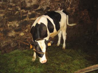
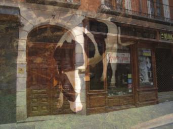
1 Chapter 4 Statistical image models 4. Introduction 4.. Visual worlds Figure 4. shows images that belong to different visual worlds. The first world (fig. 4..a) is the world of white noise. It is the world that you get to see when you watch an old TV. Images in this world can be easily described by specifying the algorithm used to generate them: create and array of n m color pixels and assign to each color component of each pixel a random number drawn from a uniform distribution between 0 and 55. In this world, all the images that belong to this world are very different in terms of the exact RGB values that make every pixel. But all the images look the same to the human visual system. The second world (fig. 4..b) is the world of random Gabor patches. It is a visual world that one gets to see when reading papers on visual psychophysics. Again, an algorithm provides the perfect description for this world: select at random N locations in the image and place at each location,a Gabor patch with a random orientation. These images look a lot more interesting to the human eye even though they contain a lot less detail than images from the first world. The third world (fig. 4..c) is the world of Mondrian paintings. This world is more visually appealing. It contains structures that the eye loves. To the point that some people have made a lot of money by generating samples from this visual world. In its most simplistic form, the images that belong to this set can be described as a random set of squares with random sizes and locations. The squares are drawn in a random order, generating a random pattern of occlusions among them. The fourth visual world (fig. 4..d) is the world of outer space images. This visual world, despite that it appears as being relatively simple, at least visually, it is not. However giving an exact algorithm to produce images from this set is quite challenging, but doable. One good approximation is to generate images by randomly placing a small number of small dots on a black background. A better algorithm will requite modeling star dynamics, gravity, etc. The fifth visual world (fig. 4..e) is the world of clouds. This visual world is visually simple, but it is hard to put into words a description of how images of this set should be generated. One can describe the images as images of clouds but that description will be hardly useful. The sixth world (fig. 4..f) is the world of line drawings of real scenes. The images in this set contain a sparse set of thin dark lines on a white background. Going beyond that description is hard. One could also add that the lines are organized to depict real world places and that they seem to correspond to important boundaries of objects in the world. But that definition is not a good procedural description, and it also feels incomplete (some of the lines do not necessarily correspond to object boundaries).

2 a) b) c) d) e) f) g) h) Figure 4.: Different visual worlds, some real, some synthetic. a) white noise, b) stars, c) gabor patches, d) mondrian, e) clouds, f) line drawings, g) CGI, e) a real street. All these worlds have different visual properties. Even there is something that makes CGI images distinct from pictures of true scenes. The seventh world (fig. 4..g) is the world of realistic scenes rendered with cheap computer graphics. Because the images are generated with computer graphics, there is a procedure that one can follow to generate them. But the procedure lacks the simplicity of the previous visual worlds. The images in this set contain the complexity of real pictures. But there is something missing, something that makes that image to look like what it really is: a cheap CGI. The eight world (fig. 4..h) is the set of typical images that one can take by taking pictures of the real world. Explaining what makes images in this set different to all other images is not an easy task. One important observation is that we can clearly differentiate images as belonging to any of these 8 worlds, even if those visual worlds look like nothing we normally when walking around... In this lecture we will talk, in some way or another, about all these visual worlds. The goal of this lecture is to present a set of models that can be used to describe images with different properties. We will describe models that can be used to capture what makes special each visual world. Even if the models we will discuss will not be as accurate as the models for the visual worlds a-c, we will show that the models can be descriptive enough to be useful in a number of applications. These models can be used to separate images into different causes, to do image denoising, superresolution, Separating images into components One of the reasons why it is interesting to understand the properties of different sets of images is because many perceptual tasks can be formulated as separating an input image into a collection of images, each one describing a different image property. Figure 4. shows four examples on input images and their decomposition. The first example shows a normal photograph corrupted by noise. Our visual system is able to notice that this image is not normal and that it is corrupted by noise. We do not perceive this scene as being composed by objects covered with a strange form of paint. We see that there is noise and it is not

3 = + = - = * = + Figure 4.: The goal is to separate each image into several images.

4 Figure 4.3: Telling noise from texture. Which one is which? supposed to be there, it is not part of the real scene. What we will like is to be able to remove the noise from the image automatically. This is equivalent to be able to separate the image into two components, one looking like a clean uncorrupted picture of a street and the second image containing only noise. How do we tell noise from texture? Figure 4.3 shows two scenes one contains noise, and the other objects textured with noise. Can you tell which one is which? Where is the noise? in the image or in the world? Image noise does not follow the objects, does not deform with the 3D surfaces, it does not change frequency with distance,... If the noise was really in the world, stationary noise will require a special noise distribution that conspires with the observer view point to appear stationary. The second example shows a blurry image. This image can be decomposed into a full resolution image from which we remove the high spatial frequencies from it. Again, we do not perceive the blurry image as a normal picture of a scene composed by objects with fuzzy boundaries. The third example shows an image mixes with a ramp (which could model illumination effects), and the fourth image is the sum of two normal images (additive transparency). Again, we have a very vivid impression of transparency. Separating an image into different causes it is an important vision task. It is important to note that the separation into these components does not rely on our ability to recognize objects and scenes (at least not totally). It seems to rely on more basic mechanisms. It is easy to see that this task can not be solved without making some assumptions. The problem we are trying to solve is like trying to find a and b given the next equation: 4 = a b (4.) In the rest of the lecture we will see models of images that will provide the tools needed to separate images into components, without recognition. 4. A sequence of statistical models of images There is a significant interest in building image models that can represent whatever makes special real photographs relative to, let s say, images that just contain noise. One way of building an image model

5 is by having some procedural description, for instance a list of objects with locations, poses and styles and a rendering engine, just like one would do when writing a program to generate CGI. One issue with this way of modeling images is that it will be hard to use it, and will require having an exhaustive list of all the things that we can find in the world. We will see later in the class that the apparent explosion in complexity should not stop us. However there is another way of building image models. In the rest of this lecture we will study a very different approach that consists in building statistical models of images that try to capture the properties of small image neighborhoods. Statistical models are very successful in other disciplines such as natural language modeling. Here we will review models of images of increasing complexity starting with the simplest possible neighborhood: the pixel. 4.. Histograms The simplest image model will consist in assuming that all pixels are independent and their intensity value is drawn from some distribution. We can write this as: p(i) = x,y p(i(x, y)) (4.) We will see the interest of writing models in this form. One way of getting a sense of how accurate is a statistical image model is to sample from this model and check the types of images that it produces. This will require knowing the distribution p(i(x, y)) (we will assume this function is the same in all image locations). What we can do is to take one image from one of the visual worlds that we described in the introduction, we can then estimate the function p(i(x, y)) as the histogram of the image. We can then sample new images from eq. 4.. Figure 4.4 shows two pairs of images with matched intensity histograms. We can see that this simplistic model is somewhat appropriate for pictures of stars (although star images can have a lot more structure), but it miserably fails in reproducing anything with any similarity to a street picture. Let s be honest, as a generative model of images, this model is very poor. However, this does not mean that image histograms are not important. Figure 4.5 shows examples of spheres that are reflecting some complex ambient illumination. The two spheres on the left are the two original images. The ones on the left are generated by modifying the image histograms to match the histogram of the opposite image. The figure shows that by simply changing the image histogram we can transform how we perceive the material of each sphere: from shiny to mate. Manipulating image histograms is a very useful operation. Given two images I and I with histograms h and h, we look for a pixelwise transformation f(x) so that the histogram of the transformed image, f(i ), matches the histogram of I. There are many ways in which histograms can be transformed. One natural choice is a transformation that preserves the ordering of pixels intensities. 4.. Dead leaves model In the quest to find what makes photographs of everyday scenes special, the next simplest image structure is a set of two pixels. Things get a lot more interesting now. One interesting observation is that if one plots the value of the intensity of one pixel as a function of the intensity value of the pixel nearby, The scatterplot produced by many pixel pairs (fig. 4.6) is concentrated on the identity line. As we look at the correlation between pixels that are farther away, the correlation value slowly decays. The correlation between two pixels is: C( x, y) = ρ [I(x + x, y + y), I(x, y)] (4.3)

6 x x x 0 4 x Figure 4.4: Examples of images and white noise with matched histograms. Only the image with stars has some visual similarity with pictures of stars. Figure 4.5: This is an example that illustrates the perceptual importance of simple histogram manipulations. Note how by simply modifying the image histograms, the sphere seems to be made by a different type of material. Image from Dror, Fleming, Adelson.

7 Figure 4.6: Scatter plots of pairs of pixels intensities as a function of distance, and cross-correlation function for vertical and horizontal displacements. The behavior of this correlation function when computed on natural images is very different from the one we would observe if the correlation was computed over noise images. There has been a large number of efforts trying to model what is the minimal set of assumptions that one needs to make in order to reproduce the observed behavior. The dead leaves model is a simplified image formation model that tries to approximate some of the properties observed for natural images. This model was introduced in the 60 s by Matheron (67) and popularized by Ruderman (97). This model consist in assuming that an image can be modeled as a set of disks (dead leaves) that fall on a flat surface generating a random superposition (e.g., fig. 4..c). This model is very simple and does not produce realistic images, but it is similar to the image model assumed to explain the distribution of albedos in natural images. This model is used by the Retinex algorithm to separate and image into two components: illumination and albedo variations. We will see this later. The particular form of the correlation function for natural images is made more explicit when studied on the Fourier domain. One remarkable property of most natural images is that if you take the D Fourier transform of an image, and look at the form of the magnitude seems to follow a form: Ĩ(v) v α (4.4) where v denotes spatial frequency, Ĩ is the Fourier transform of the image I, and α. And this is true for all orientations (you can think of this as taking the fourier transform and looking at the profile of a slice that passes by the origin) The gaussian model We want to write a statistical image model that takes into account the correlation statistics of natural images (see Simoncelli 005 for a review). If the only constraint we have is the correlation function among image pixels, then, among all the possible distributions the one that has the maximum entropy (maximum entropy principle) is the Gaussian distribution: ( p(i) exp ) IT C I (4.5) where C is the covariance matrix of all the image pixels. Note that now this model does not assume independency across pixels any more. This model takes into account that intensity values for different

8 Figure 4.7: Randomizing the phase of picture of clouds. Left) clouds, Center) magnitude of its Fourier transform, Right) image obtained by randomizing the phase. pixels are correlated as discussed in the previous sections. This model is related also to studies that use principal component analysis to study what are the typical components of natural images. For stationary signals, the matrix C has a circulant structure (assuming a tiling of the image) and can be diagonalized using the Fourier transform. The eigenvalues of the diagonal matrix correspond to the power (squared magnitude) of the frequency components of the Fourier transform. This is, the matrix C can be written as C =EDE T, where E is the matrix that contains the Fourier basis (as seen in the previous lecture) and the diagonal matrix D is composed by the values v α for all the frequencies v. Assumptions The gaussian model is the result of making a number of assumptions about images: Stationarity Scale invariance Sampling images Once a distribution is defined, we can use it to sample new images. First we need to specify the parameters of the distribution. In this case, we need to specify the matrix C. We can estimate this as the average covariance matrix of a set of images. Figure 4.7 shows an example of an image of clouds and the magnitude of its Fourier transform. A sample of the distribution can be obtained by filtering white gaussian noise using the image magnitude as a filter. Image denoising and Wiener filter As an example of how to use image priors for vision tasks, we will study how to do image denoising using the prior on the structure of the correlation of natural images. In this problem, we observe a noisy image I n corrupted with white gaussian noise: I n (x, y) = I(x, y) + n(x, y) (4.6) and the goal is to recover the uncorrupted image I(x, y). The noise n(x, y) is white gaussian noise with variance σ n.

9 The denoising problem can be formulated as finding I that maximizes the maximum a posteriory (MAP estimate): max p(i I n ) (4.7) I In these equations we write the image as a column vector I. This posterior density can be written as: where the likelihood function is: max I p(i I n ) = max p(i n I)p(I) (4.8) I p(i n I) exp( I n I /σ n) (4.9) and the prior: ( p(i) exp ) IT C I (4.0) The solution to this problem can be obtained in closed form: I = C ( C + σ ni ) In (4.) This is just a linear operation. It can also be written in the Fourier domain as: Ĩ(v) = A/ v α A/ v α + σn Ĩ n (v) (4.) Image deblurring If an image is blurred with a Gaussian filter of unknown variance, we can try to estimate the parameter of the gaussian blurring filter by looking at the log(ĩ) K α log( v ) v /σ (4.3) From this equation, one can try to estimate the parameters of the gaussian blurring filter.