Image Alignment AJIT RAJWADE

Size: px

Start display at page:

Download "Image Alignment AJIT RAJWADE"

Philomena Walton
5 years ago
Views:

1 Image Alignment AJIT RAJWADE

2 Basics A digital image a discrete/sampled version of a visual stimulus Can be regarded as a function I = f(,) where (,) are spatial (integer) coordinates in a domain W = [0,-] [0,W-]. Each ordered pair (,) is called a piel. The piel is generall square (sometimes rectangular) in shape.

3 Basics Piel dimensions (height/width) relate to the spatial resolution of the sensor in the camera that collects light reflected from a scene.

4 Basics In a tpical grascale image, the intensit values f(,) lie in the range from 0 to 55 (8 bit integers). The are quantized versions continuous values corresponding to the actual light intensit that strikes a light sensor in the camera.

5 Image Alignment Consider images I and I of a scene acquired through different viewpoints. Piels in digital correspondence (same coordinate values in the image domain W, not necessaril containing measurements of the same phsical point) Piels in phsical correspondence (containing measurements of the same phsical point, but not necessaril the same coordinate values in the image domain W)

6 Image Alignment I and I are said to be aligned if for ever (,) in the domain W, the piels in I and I are in phsical correspondence. Image alignment (also called registration) is the process of correcting for the relative motion between I and I.

7 Image alignment: steps First step: motion estimation Second step: image warping

8 Motion estimation

9 Motion Models Let us denote the coordinates in I as (, ) and those in I as (, ). Translation: Rotation about point (0,0) anti-clockwise through angle q t t W ), ( cos sin sin cos cos sin sin cos θ θ θ θ θ θ θ θ D Rotation matri (orthonormal matri)

10 Motion Models Rotation about point ( c, c ) anti-clockwise through angle q 0 0 cos sin sin cos cos sin sin cos c c c c c c c c c c θ θ θ θ θ ) ( θ ) ( θ ) ( θ ) ( -Perform translation such that ( c, c ) coincides with the origin. -Rotate about the new origin. -Translate back.

11 Motion Models Rotation and translation: Affine transformation: rotation, translation, scaling and shearing 0 0 cos sin sin cos cos sin sin cos c c c c c c t θ θ t θ θ t θ ) ( θ ) ( t θ ) ( θ ) ( 0 0 t A A t A A Assumption: the sub-matri A is NOT rank deficient, otherwise it will transform two-dimensional figures into a line or a point

12 Motion Models The D affine motion model (including translation in X and Y direction) includes 6 degrees of freedom. Note: this motion model accounts for in-plane motion onl (eample: not an appropriate model for head profile view versus head frontal view )

13 Motion Models Consider two images (perspective projection) of a plane in 3D space. These images are said to be related b a motion model called as a planar homograph which we studied last class.

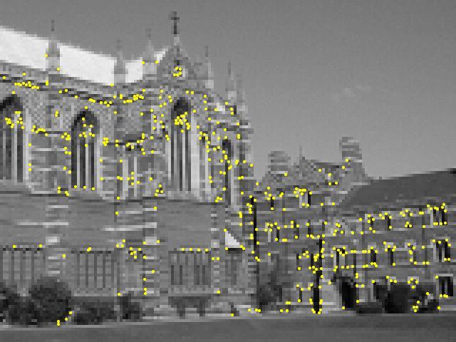
14 P Plane π p p O O

16 Motion Models summar Parametric models Motion Model DOF D rigid +=3 D similarit (rigid+ uniform scaling) D affine 6 omograph 8 3D rigid 6 3+=4 3D similarit 6+=7 3D affine D (or 3D) non-parametric (also called non-rigid or deformable ) number of piels (or 3 number of voels)

17 Alignment with control points Solve for unknown parameters using leastsquares framework (i.e. pseudo-inverse) Appl the motion based on these parameters to the first image Control points: pairs of phsicall corresponding points mabe marked out manuall, or automaticall using geometric properties of the image. Number of control points N MUST be >= u/, where u = number of unknown parameters in the motion model (each point has two coordinates and ) A A 0. A A k k t t k k

18 Least squares motion estimation: affine For the affine model, we can write the earlier equation as follows: * * arg min ) ( F A noise A P P PP P P A AP P T T 0 0 t A A t A A A i j F X ij X ) ( 0 ) ( ( ) ( ) ( T T T PP P P A P AP P A AP ) AP P A AP P A E E F

19 Least squares motion estimation: homograph For the homograph motion model, we have previousl seen that the solution is given as follows: has size 9 9, has size ; s.t. arg min * h A h A h h Ah h h N i i i i i i i i i i i i i i t

20 Least squares motion estimation: rigid motion For the rigid motion model, we can write the earlier equation as follows: P RP t noise ( R*, t* ) arg min P RP t ( R, t) F s.t. R T R I This problem cannot be solved correctl b a simple pseudoinverse because a pseudo-inverse does not impose the fact that R is an orthogonal matri. The correct solution uses the singular value decomposition. It is detailed here below assuming that t = 0 (the solution can be etended to the case where t is not 0) Also see:

21 Segwa: Singular value Decomposition For an m n matri A, the following decomposition alwas eists: A USV U V T T U V S R mn T UU VV, A R T T I m I n mn,,u R,V R mm nn,, Diagonal matri with nonnegative entries on the diagonal called singular values. T Columns of U are the eigenvecto rs of AA (called theleft singular vectors). T Columns of V are the eigenvecto rs of A A (called the right singular v ectors). The non - zero singular values are the positivesquare roots of non - zero eigenvalue s of AA T or A T A.

22 Marking control points Control points (also called feature points, salient points, fiducials or salient feature points) can be manuall marked which is error-prone and tedious. owever this process can also be automated b using salient feature point detectors which are invariant to geometric transformations. An ecellent eample of this is SIFT (scale invariant feature transform).

23 Marking control points: SIFT SIFT does two things: it detect salient points in each image and associates each salient point with a feature vector. The feature vector is a characteristic of a small region of the image around the salient point. The feature vector for each salient point is provabl invariant to translation, rotation and reflection and approimatel (or as observed empiricall) invariant to affine transformations and even some perspective changes. The feature vector is also provabl invariant to several illumination changes of the form I = ai + b. where I and I are observed intensities, and a,b are coefficients (constant for the whole image). It is empiricall seen to be invariant to man other tpes of illumination changes.

25 Marking control points: SIFT Due to this invariance, the SIFT technique is able to do a good job at matching salient points from one image to another. The motion model can then be estimated from the matched points.

26 Image warping

27 Image warping After motion estimation, the net step is to warp one of the images (sa) I using the estimated motion represented b a matri (sa T).

28 Forward warping: Image Warping -Appl the motion Tv to ever coordinate vector v = [ ] in the original image (i.e. I ). -Cop the intensit value from v in I to the new location (Tv) in the warped image. If the new location is not an integer (most likel), then round off to nearest integer. I (, ) I warped (round(tv))

29 Forward warping: Image Warping -Can leave the destination image with some holes if ou scale up. -Can lead to multiple answers in one piel if ou scale down.

30 Image Warping Reverse warping: Note: this assumes that T is an invertible transformation, which is guaranteed in the applications we are dealing with. It is not guaranteed in case of non-rigid deformations, given the pielized (i.e. discrete) image coordinate sstems. -For ever coordinate v = [ ] in the destination image, cop the intensit value from coordinate T - v in the original image. In case of non-integer value, perform interpolation (nearest neighbor or bilinear) I (T - (, )) I warped (, )

31 Interpolation a a4 A D B C A,B,C,D denotes Areas of these four rectangles a a3 Nearest neighbor method: Use value a 4 (as the piel that is nearest to the red point contains value a 4 ) Bilinear method: Use the following value, a weighted combination of the four neighboring piel values, with more weight to nearer values: Ba4 Aa3 Ca ( A B C Da D) Ba 4 Aa 3 Ca Da I (T - (, )) I warped (, )

32 Warping with homographies Consider the equation: While warping, note the division b w to ield,im and,im. This is different from the affine case! 33, 3, 3 3,, ,,, 33, 3, 3 3,, ,,, ,, w v u w v u w v w v w u w v u w v u w u w v u w v u im im im im im im im im im im im im im im im, im, p p

33 Image alignment using image similarit measures (without using control points)

reliabl matched from one image to another.

34 Control points are not alwas available In some scenes, good control points ma not be available Or the cannot sometimes be reliabl matched from one image to another. Eample: some modalities such as ultrasound, or images that are heavil blurred or nois.

35 Alignment with mean squared error Mean squared error is given b: MSSD N, W ( I (, ) I(, )) Find motion parameters as follows: T T * arg min A A 0 A A 0 MSSD T ( I t t, v ( v), I ( Tv)) Find transformation matri T which produces the least value of MSSD I = called the fied (or reference) image I = called the moving image

36 Alignment with mean squared error For simplicit, assume there was onl rotation and translation. Then we have T T * arg min MSSDT ( I( v), I( Tv)) cosq sinq 0 sinq cosq 0 t t, v

37 Alignment with mean-squared error There are man was to do this minimization. The simplest but inefficient wa is to do a brute-force search. Sample q, t and t uniforml from a certain range (eample: q from -45 to +45, t or t from -30 to +30). Appl this motion to I keeping I fied, and compute the MSSD. Each time, compute the MSSD. Pick the parameter values (i.e. q, t and t ) corresponding to minimum MSSD.

38 Alignment with mean squared error In the ideal case, the MSSD between two perfectl aligned images is 0. In practice, it will have some small non-zero value even under more or less perfect alignment due to sensor noise or slight mismatch in piel grids.

39 Careful: field of view issues! Fied image Region of overlap when the moving image is warped Note: compute MSSD onl over region of overlap.

40 Change in region of overlap, as the moving image is warped

41 Alignment with mean squared error MSSD is one eample of an image similarit measure. MAJOR ASSUMPTION: Phsicall corresponding piels have the same intensit, i.e. the are acquired b similar cameras and under the same lighting condition (this is often called as mono-modal image registration).

42 Image alignment: Intensit changes in images Images acquired b different sensors (MR and CT, different tpes of MR, camera with and without flash, etc.) Changes in lighting condition This is called as multimodal image registration. MR-PD MR-T

43 /Flash_%8photograph%9 #mediaviewer/file:fill_flash. jpg upenn.edu/sbia/s oftware/dramms/ tutorials/prostate istmri.html

44 Image alignment: Intensit changes in images If following relationship eists and we knew the eact functional form (sa g), the solution is eas: I (, ) g( I(, )), (, ),(, ) W Phsicall corresponding points transformed MSSD N, W ( g( I (, )) I(, ))

45 Image alignment: Intensit changes in images What if the relationship eists in the following linear form, but we knew it onl partiall? Phsicall corresponding points; a and b are unknown, but we know the relationship is linear ), ( ), ( ), (, images of value average :, ) ), ( ( ) ), ( ( ) ), ( )( ), ( ( I I I I I I I I I I I I NCC W W W W ), ),(, (, ), ( ), ( b ai I Normalized cross-correlation, also called correlation-coefficient observe its relation to a noramlized vector dot product. We are taking the absolute value here, to take care of cases where one image has positive values and the other has negative values

46 Image alignment: Intensit changes in images Normalized crosscorrelation, also called correlation-coefficient ), ( ), ( ), (, images of value average :, ) ), ( ( ) ), ( ( ) ), ( )( ), ( ( I I I I I I I I I I I I NCC W W W, 0 0 )) ( ), ( ( arg ma * t A A t A A I I NCC v T Tv v T T

47 Image alignment: intensit changes in images? Assume there eists a functional relationship between intensities at phsicall corresponding locations in the two images. But suppose we didn t know it (most practical scenario) and couldn t find it out. We will use image histograms!

48 Image istogram In a tpical digital image, the intensit levels lie in the range [0,L-]. The histogram of the image is a discrete function of the form P(r k ) = n k /W, where r k is the k-th intensit value, and n k is the number of piels with that intensit. Sometimes, we ma consider a range of intensit values for one entr in the histogram, in which case r k = [r min k, r ma k] represents an intensit bin, and n k is the number of piels whose intensit falls within this bin. Note P(r k ) >= 0 alwas, and all the P(r k ) values sum up to.

49 Joint Image istogram Function of the form P(r k,r k ) where r k and r k represent intensit bins from the two images I and I respectivel. P(r k,r k ) = number of piels (,) such that I (,) and I (,) lie in bins r k and r k respectivel, divided b W.

50 Consider two 3 3 images above for eample sake. Their joint histogram is as follows: P(4,) = /9 P(,) = /9 P(3,6) = 3/9 P(6,3) = /9 P(,4) = /9 P(4,) = /9

I 0 Values in I from 0 to 60 I 60 0 60 Values in I (from 0 to 60) Registered

The joint histogram is plotted as a grascale image.

51 I 0 Values in I from 0 to 60 I Values in I (from 0 to 60) Registered images: joint histogram plot looks streamlined ow was this plot generated? The joint histogram is plotted as a grascale image. Brighter points in this image indicate larger probabilities and darker points indicate lower probabilities.

0 Values in I from 0 to 60 60 0 60 Values in I

52 0 Values in I from 0 to Values in I (from 0 to 60) Misaligned images: joint histogram plot looks dispersed We need a method to quantif how dispersed a joint histogram actuall is.

53 Values in I (0 to 60, top to bottom) Values in I (0 to 60) Misaligned images: the joint histogram plot appears dispersed. We need a method to quantif how dispersed a joint histogram actuall is.

54 Measure of dispersion Consider a discrete random variable X with normalized histogram P(X=) [also called the probabilit mass function]. The entrop of X is a measure of the uncertaint in X, given b the following formula: ( X ) P( X )log DX DX discrete set of values P( X that can E( log( P( X take Entrop is a function of the histogram of X, i.e. of P(X). It is not a function of the actual values of X. The entrop is alwas non-negative. X ) ))

55 Entrop The entrop is maimum if X has a discrete uniform distribution, i.e. P(X=) = P(X=) for all values and in DX. The maimum entrop value is log( DX ). The entrop is minimum (zero) if the normalized histogram of X is a Kronecker delta function, i.e. P(X= ) = for some, and P(X= ) = 0 for all.

56 Joint entrop The joint entrop of two random variables X and Y is given as follows: ( X, Y ) P( X, Y )log DX DY P( X Maimum entrop: -Uniform distribution on X and Y: entrop value log( DX DY ) Minimum entrop: -Kronecker delta, i.e. P(X=,Y= ) = for some, and P(X=,Y= ) = 0 for all or., Y )

57 Joint entrop Minimizing joint entrop is one method of aligning two images with different intensit profiles., 0 0 )) ( ), ( ( arg min * t A A t A A I I v T Tv v T T

58 I I : obtained b squaring the intensities of I, and rotating I anticlockwise b 30 degrees. I treated as moving image, I treated as fied image. Joint entrop minimum occurs at -30 degrees.

59 Image Alignment: Application Scenarios

60 Image Alignment: applications, related problems Template matching Image Panoramas Denoising image-bursts Collecting photos of paintings Face recognition 3D-D image registration

61 () Template Matching Look for the occurrence of a template (a smaller image) inside a larger image. Eample: ees within face image Templates

62 () Image Panoramas ch.html

63 ftp://ftp.math.ucla.edu/pub/camreport/cam09-6.pdf,buades et al, A note on multi-image denoising (3) Denoising image bursts An image burst is a collection of photos (of the same scene) taken in quick succession, each with ver short eposure time. Each image is sharp but usuall quite nois (even more so if the lighting was poor). Due to camera motion during burst acquisition, the images can be slightl misaligned. You can align the images (sa using SIFT for the control points and assuming a homograph motion model) and then simpl average the images after alignment to remove the noise.

64 Image bursts are tpicall used for photographing fast moving objects (water fountains, sports, children). ere, however, we use it for photograph under poor lighting conditions. photograph%9

66 (4) Photographing paintings The Google Art Project ( sought to acquire high-resolution photographs of paintings from famous museums. Acquiring such photographs requires ver specialized equipment, controlled illumination and intensive postprocessing. The major problem in photographing a painting is that different portions of the painting ehibit a glare, depending on the viewpoint in which the picture was taken. If the painting is behind a glass/plastic frame, one sometimes sees the reflection of the observer in it. These glares and reflections change their location, if ou change the viewpoint in which the picture was taken.

See: http://www.siam.org/publicawareness/art.

67 See:

68 See:

69 (4) Photographing paintings In an approach proposed b aro, Buades and Morel ( ), one takes several bursts of pictures of the painting from different viewpoints. All these images are aligned together using SIFT+homograph. This is followed b image fusion, i.e. computing an average or median of all aligned images (the paper actuall does this differentl, but that is not so important in the present contet of image alignment).

71 (5) Face recognition In a face recognition application, ou first store one or more images of each person (sa students/staff at IITB) in a database. These are called galler images. Given an image of a person at some later point of time, the task is to match the image to the set of galler images in order to determine identit. This is called the probe image. The probe image can be in a different pose than the galler image of the same person.

72 (5) Face recognition If the galler and pose image had onl inplane motion relative to each other, we could use one of the earlier discussed methods to find the unknown motion. Eample below:

motion. What does one do then? http://www.cs.

73 (5) Face recognition But this does not handle the much more realistic issue of out-of-plane motion. What does one do then? edu/~jebara/htmlpapers /UTESIS/node30.html

(6) 3D-D registration This motivates the use of 3D face scans or 3D models which can be acquired b 3D cameras such as stereo-cameras or structured light sensors.

74 (6) 3D-D registration This motivates the use of 3D face scans or 3D models which can be acquired b 3D cameras such as stereo-cameras or structured light sensors. A 3D face scan consists of a set of vertices in 3D and a set of polgons (in 3D) linking those vertices.

75 (6) 3D-D registration Given the 3D model of a person, ou need to match the probe image to the model. ow? You create images b projecting the 3D model in different viewing directions, and then match each image with the probe image. ow man DoF involved? Si: direction of viewing (), distance of viewpoint along the viewing direction (), direction measured to which offset point in 3D (another 3). glulookat.html

Source: PhD thesis of Paul Viola at MIT (995) http://research.microsoft.com/pubs/667/phd-thesis.

76 Source: PhD thesis of Paul Viola at MIT (995) The method emploed was optimization of mutual information (closel related to the joint entrop technique) we studied in class.

77 What we learnt.. Affine motion model Forward and reverse image warping Field of view during image alignment Measures for Image alignment: sum of squared differences, normalized crosscorrelation, joint entrop Registration using control points

78 What we didn t learn Complicated motion models: higher degree polnomials, non-rigid models (eample: motion of an amoeba, motion of the heart during the cardiac ccle, facial epressions, etc.) Efficient techniques for optimizing the measure for image alignment

79 Aspects of image registration Are the images in D or in 3D? (D-D, 3D-3D, 3D-D) Is the motion model parametric or nonparametric (non-rigid)? Do the images have equal intensit values at phsicall corresponding points? (Unimodal or multimodal). This decides the objective function to be optimized.

CS 2770: Intro to Computer Vision. Multiple Views. Prof. Adriana Kovashka University of Pittsburgh March 14, 2017

CS 2770: Intro to Computer Vision. Multiple Views. Prof. Adriana Kovashka University of Pittsburgh March 14, 2017 CS 277: Intro to Computer Vision Multiple Views Prof. Adriana Kovashka Universit of Pittsburgh March 4, 27 Plan for toda Affine and projective image transformations Homographies and image mosaics Stereo