CALIFORNIA STATE UNIVERSITY, NORTHRIDGE LOSSLESS COMPRESSION OF SATELLITE TELEMETRY DATA FOR A NARROW-BAND DOWNLINK

Transcription

1 CALIFORNIA STATE UNIVERSITY, NORTHRIDGE LOSSLESS COMPRESSION OF SATELLITE TELEMETRY DATA FOR A NARROW-BAND DOWNLINK A graduate project submitted in partial fulfillment of the requirements For the degree of Master of Science in Electrical Engineering By Gor Beglaryan May 2014

2 Copyright Copyright (c) 2014, Gor Beglaryan Permission to use, copy, modify, and/or distribute the software developed for this project for any purpose with or without fee is hereby granted. THE SOFTWARE IS PROVIDED "AS IS" AND THE AUTHOR DISCLAIMS ALL WARRANTIES WITH REGARD TO THIS SOFTWARE INCLUDING ALL IMPLIED WARRANTIES OF MERCHANTABILITY AND FITNESS. IN NO EVENT SHALL THE AUTHOR BE LIABLE FOR ANY SPECIAL, DIRECT, INDIRECT, OR CONSEQUENTIAL DAMAGES OR ANY DAMAGES WHATSOEVER RESULTING FROM LOSS OF USE, DATA OR PROFITS, WHETHER IN AN ACTION OF CONTRACT, NEGLIGENCE OR OTHER TORTIOUS ACTION, ARISING OUT OF OR IN CONNECTION WITH THE USE OR PERFORMANCE OF THIS SOFTWARE. Copyright by Gor Beglaryan ii

3 Signature Page The graduate project of Gor Beglaryan is approved: Prof. James A Flynn Date Dr. Deborah K Van Alphen Date Dr. Sharlene Katz, Chair Date California State University, Northridge iii

4 Contents Copyright... ii Signature Page... iii List of Figures... vi List of Tables... viii ABSTRACT... ix 1 Introduction Background: Information Theory and Coding Outline Formulas and Measures of Performance Lossy vs. Lossless Compression Design Procedure Problem Definition Huffman Codes How Huffman Codes Work Huffman Algorithm Design Efficiency of Huffman Compression Sample Output of the Static Huffman Algorithm Adaptive Huffman Codes How Adaptive Huffman Codes Work Adaptive Huffman Algorithm Design Efficiency of Adaptive Huffman Codes Sample Output of the Adaptive Huffman Algorithm Arithmetic Coding How Arithmetic Coding Works Arithmetic Coding Algorithm Design Efficiency of Arithmetic Coding Sample Output of the Static Arithmetic Algorithm Adaptive Arithmetic Coding How Adaptive Arithmetic Coding Works Efficiency of Adaptive Arithmetic Coding Performance Tests and Comparison Pic33 Analog-to-Digital Converter Output Format iv

5 4.2 Benchmark Test Test Data Compression Ratio Test Timing Test Discussion of Test Results Delta Compression Conclusions Bibliography Appendix A: MATLAB Code for Static Huffman Compression Appendix B: MATLAB Code for Adaptive Huffman Compression Appendix C: MATLAB Code for Static Arithmetic Coding Appendix D: MATLAB Code for Adaptive Arithmetic Coding Appendix E: MATLAB Code for 10 bit Conversion Appendix F: MATLAB Code for 12 bit Conversion v

6 List of Figures Figure 2.1-Simplified source and channel coding system Figure 3.1-Static Huffman compression flowchart Figure 3.2-Huffman binary tree example Figure 3.3-Flowchart for traversing a binary tree Figure 3.4-Static Huffman compression output format Figure 3.5-Encoded binary tree example Figure 3.6-Output variable info of the Static Huffman program Figure 3.7-Output variable info.codewords of the Static Huffman program Figure 3.8-Histogram generated by the Static Huffman Program Figure 3.9-Adaptive Huffman encoding flowchart [15] Figure 3.10-Adaptive Huffman tree example Figure 3.11-Adaptive Huffman tree node update example Figure 3.12-Adaptive Huffman compression output format Figure 3.13-Adaptive Huffman decoder flowchart [17] Figure Output variable info of the Adaptive Huffman program Figure 3.15-Final binary tree table of the Adaptive Huffman simulation Figure 3.16-Output variable info.codewords of the Adaptive Huffman program Figure 3.17-Generating unique tag for Static Arithmetic Coding Figure 3.18-Arithmetic Coding Case 0 and Case 1 rescaling [23] Figure 3.19-Arithmetic Coding Case S rescaling [23] Figure 3.20-Static Arithmetic Coding flowchart Figure 3.21-Static Arithmetic Coding output format Figure 3.22-Static Arithmetic Coding output example Figure 3.23-Static Arithmetic decoder flowchart Figure 3.24-Output of the Static Arithmetic program Figure 4.1-dsPic33 ADC Output Format Figure 4.2-Data conversion from input to output Figure 4.3-Symbol histogram of the book of Genesis Figure 4.4-Sample indoor temperature data Figure 4.5-Sample outdoor temperature data Figure 4.6-Sample wind speed data Figure 4.7-Sample wind gust data Figure 4.8-Sample magnetic field data Figure 4.9-Compression results for the book of Genesis Figure 4.10-Compression results for indoor temperature data Figure 4.11-Compression results for outdoor temperature data Figure 4.12-Symbol histogram for indoor and outdoor temperature data source alphabet Figure 4.13-Compression results for magnetic field data Figure 4.14-Compression results for wind gust data Figure 4.15-Compression results for wind speed data Figure 4.16-Compression time results (linear scale) Figure 4.17-Compression time results (logarithmic scale) vi

7 Figure 4.18-Decompression time results (linear scale) Figure 4.19-Total compression and decompression time (linear scale) Figure 4.20-Total compression and decompression time (logarithmic scale) vii

8 List of Tables Table 2.1-Information theory and coding: outline of topics... 3 Table 3.1-Table for storing Huffman Tree Table 3.2-Table for storing Adaptive Huffman tree Table 3.3-Source alphabet information of the sequence "abracadabra" viii

9 ABSTRACT LOSSLESS COMPRESSION OF SATELLITE TELEMETRY DATA FOR A NARROW-BAND DOWNLINK By Gor Beglaryan Master of Science in Electrical Engineering The objective of this project is to select a lossless compression technique to be implemented on a CubeSat being developed by CSUN. The goal is to compress satellite telemetry data in a timely and computationally efficient manner and achieve reasonable compression ratio. There are two main parts in this project; Algorithm Development and Benchmark Tests. In the former phase four lossless compression techniques, namely Huffman, Adaptive Huffman, Arithmetic and Adaptive Arithmetic, were implemented in MATLAB. Concise description and implementation details of each algorithm are given in the text. Next, during the Benchmark Test phase, sample data is input to the algorithms and performance metrics are collected. The collected performance measures include compression ratio, compression time and decompression time. Based on the results, it is recommended that Adaptive Arithmetic coding be selected for the CubeSat project. ix

10 1 Introduction CubeSats are small satellites between 1000 and 3000 cm 3 in volume. They are a low cost method for conducting experiments in space. Due to the size, weight, power limitations and orbit of these small satellites the downlink data rates are often limited. Thus, it may be necessary to compress the data on the satellite before it is transmitted. This project is a study of some of the lossless compression schemes that might be used. In order to select a lossless compression technique, four algorithms, each representing a different compression method, have been implemented in MATLAB. All algorithms perform necessary data manipulation, parsing, compression, decompression and original data recovery. These routines and subroutines enable modeling of an actual encoder and decoder, hence aiding in simulation and comparison of each compression method. As a result the most suitable and efficient algorithm can be selected for further analysis and possible implementation on the CubeSat. Section 2 of this report presents some background information on Information Theory and Coding that was needed to complete this project. Section 3 presents the four coding techniques that were studied and the algorithms for their implementation. Section 4 presents the benchmark tests and compares the coding techniques. Section 5 includes the conclusions and suggestions for future work. 1

11 2 Background: Information Theory and Coding With the introduction of the personal computer in the 1970s and the establishment of the Internet in the 90s, the Information Age had begun and was gaining large momentum very rapidly. As it is now known, this revolution resulted in an exponential growth of accessible information for the general public; this growth is still ongoing. This information is in the form of music, pictures, video, satellite telemetry data, medical imaging data, and a vast array of multimedia formats we encounter in our daily life. It is fair to say that this would not be possible without data compression. Before the Information Age data compression was mainly in the radar of a small group of engineers who had already developed modern compression techniques, such as Huffman Compression [1]. However, as the number of data sources expanded, the need for larger storage expanded as well. New compression techniques were needed that could significantly reduce the number of bits required for storage. 2.1 Outline Data compression, commonly referred to as source coding, is a sub-field of Information Theory and Coding. To better understand the role of data compression in the field of information theory consider Table 2.1 [2]. The table shows that data compression is applied to the source, to reduce the information size to be transmitted. In contrast, error correction is performed to transfer information reliably over a non-ideal channel that is subject to noise and other forms of distortion depending on the channel. These different components can be visualized in the simplified source and coding system shown in Figure

12 Furthermore, compression itself can be approached from two different angles, mathematical and algorithmic. The mathematical part is purely analytical and deals with Compression/Source Coding (efficiency) Error-Correction/Channel Coding (reliability) Information Theory (math) Coding methods (algorithms) i. Source coding theorem i. Noisy channel coding theorem ii. Kraft-McMillan inequality ii. Channel capacity theorem iii. Rate-distortion theorem iii. Typicality & AEP i. Symbol codes, e.g. i. Hamming codes Huffman codes ii. Turbo codes ii. Stream coder, e.g. iii. Gallager codes Arithmetic coding, iv. BCH codes, e.g. Lempel-Ziv coding Reed-Solomon codes Table 2.1-Information theory and coding: outline of topics. Figure 2.1-Simplified source and channel coding system. theorems that help to measure performance and shed light on the limitations of compression. The algorithmic perspective is a hands-on approach trying to overcome the limitations by creating complex compression packages that can manage a variety of data formats with reasonable performance. 3

13 2.2 Formulas and Measures of Performance Studying information theory and coding can quickly lead into depths that are outside the scope of this project. However, some fundamental formulas are necessary to have a basic understanding of how information is measured, how much the source data can be compressed with a given compression technique and how reliably the data can be recovered. When speaking of information theory it is essential to know how information is measured and what it represents. If ( ) is the probability that the event A will occur, then the self-information associated with A quantifies the uncertainty of the event and is given 1 i(a)=log b P(A) =- log P(A) (2.1) b by [3]. Equation 2.1 shows that the self-information of an event is a positive quantity. Moreover, the smaller the probability of the event, the higher the information. In other words, if an event is not expected to happen, the information gained would be high if it actually happened, or equivalently if an event has high probability of occurrence then there is little uncertainty associated with the event. Probability and uncertainty of an event are inversely proportional. Self-information is measured in bits. The self-information in Equation 2.1 is for a single event that leads to the average self-information of an experiment consisting of a number of independent events. This quantity is called entropy [4] and is calculated by: ( ) = ( ) ( ) (2.2) Entropy quantifies the uncertainty of an experiment. 4

14 The next formula describes the expected code-word length of a particular compression technique, which is the average code-word length of a coding scheme. The expected code length is a performance measure that can never exceed the entropy, which = ( ) (2.3) is the lower bound of the average code length. The difference between H(S) and is defined as redundancy [5], also an important measure of performance. ( ) in Equation 2.3 is the probability of the i th symbol and is the length of the code-word corresponding to it. The last, but probably the most important measure of performance is the compression ratio that can be achieved with a particular compression scheme. Compression ratio expresses the reduction in the amount of data required as a percentage of the original data size [6]. 2.3 Lossy vs. Lossless Compression Data compression can be done in two ways, lossy and lossless. As the name suggests, data that has undergone lossy compression cannot be fully recovered during decompression. In the era of analog technology lossy compression was inevitable. As soon as an analog signal is quantized, information is lost that cannot be recovered. However, in some applications, such as radiology, small details must be preserved. This became relatively easier with digital technology and lossless compression techniques. The title of this document gives away that the focus here is lossless compression of satellite telemetry data. In the next chapter a few of these lossless compression techniques will be discussed. 5

15 The information mentioned so far is for introduction only and does not even touch the tip of the iceberg when speaking of information theory in general, and data compression specifically. For a deeper insight into the theory, please see the resources mentioned in [7], [8], [9]. 6

16 3 Design Procedure 3.1 Problem Definition The basis for this project is to select a lossless compression algorithm that will be implemented on the CubeSat. Once launched and in orbit, the eleven sensors on board the CubeSat will take one measurement per second for at least one hour a day. The measurements will be taken by voltage, current and temperature sensors. The analog-to-digital converter (ADC) on the Microchip dspic33 microcontroller used on the CubeSat supports 10 or 12 bit output formats [10]. Since the data logged by the sensors is not going to have a large range, 10 bit ADC resolution is sufficient for the output. A simple calculation shows that, at a bare minimum, there will approximately be 387 of measurement data to be transmitted per day. Taking all these factors into consideration, the compression algorithms have to be able to meet the following requirements i. Lossless compression, ii. Compress at least 387 kb of data, iii. Support 10 bit data size, iv. Support 12 bit data size (if needed), v. Time efficient, vi. Memory efficient, vii. Computationally not complex. 7

17 The last three items will be quantified later when the different algorithms are compared in a benchmark test. For this project four compression techniques have been considered; Static Huffman, Adaptive Huffman, Static Arithmetic and Adaptive Arithmetic. 3.2 Huffman Codes Huffman compression is one of the first modern compression techniques. Huffman codes are probabilistic in nature, meaning that a source symbol probability distribution is necessary for generating the code-words How Huffman Codes Work In a Huffman code each source symbol is mapped to a code-word, which will replace the source symbol during encoding. In essence, this is similar to Morse code; the Figure 3.1-Static Huffman compression flowchart. 8

18 higher the probability of a symbol, the shorter the corresponding code-word. Please note that the source symbols constitute the source alphabet. The source symbols of this text are the ASCII characters. The flowchart in Figure 3.1 shows the steps necessary to map source symbols to code-words. To demonstrate this with an example, an imaginary source can be assumed that has 5 symbols. For convenience, the source alphabet is denoted as,,,, and the corresponding probability distribution is given by 0.2,0.35,0.2,0.1,0.15. Following the steps in the flowchart the values have to be sorted in decreasing order, and the symbols with the smallest two probabilities have to be combined until 1 symbol is left. The result is known as a binary tree, as shown below. The final step necessary to generate the codewords is to traverse the tree from the bottom to the top and assigning 0s and 1s on a left and right turn, respectfully. The resulting codebook is = 10, = 00, = 11, = 011, = 010, where is the code-word for symbol, etc. The resulting binary tree is shown in Figure 3.2. Figure 3.2-Huffman binary tree example. 9

19 3.2.2 Huffman Algorithm Design In this section the actual design of the Huffman algorithm is described. The flowchart in Figure 3.1 suggests that the first step in a Huffman algorithm is to sweep through the source data and count the number of occurrences of each source symbol. From this information the source symbol probabilities are easily calculated. For this purpose, a MATLAB function has been written that sweeps through the data and outputs the unique symbols and their frequencies in a two column matrix. The rows of this matrix represent the symbols that are present in the source. This function is called get_freq_huff and the code can be found in Appendix A. The get_freq_huff function returns the output variables in sorted and tabulated order. As a result, separate processing steps are not necessary to sort the probabilities in decreasing order. All programing languages offer functions or tools to extract the minimum value from a data set. So, the second step of the algorithm is to recursively find the two smallest probability entries in the table, add them together, and assign this probability to a new symbol in the table. The algorithm must also be able to trace the merger of symbols back to their original state, therefore every time there is a new table entry, two pointers are assigned that are going to point to the indices of the two symbols that have been merged to create the new table entry. A suitable pseudo code that can create and manage such a table, or multidimensional array can be found in [11]. Each entry in the table is called a root. The two roots with the smallest probabilities are combined to create a new entry in the table. This new entry has probability equal to the sum of the probabilities of the merged roots. Then the two roots are removed from the table. However, the new entry has two pointers, one for each of the previous roots, which 10

20 are now called nodes. This continues until the top root has been reached and the sum of probabilities equals 1. The pseudo-code is shown below where T is the table. Each row of the table is enclosed in the square brackets and is separated from the other row by a comma. The symbols for each row are designated by, and the associated probability is ( ), where is the symbol index. The left and right arrows are place holders for the left and =, ( ),,,, ( ),,,,, ( ),, { h >1 =min = =min = =, ( ) + ( ),, = } right children respectively. In the actual algorithm the arrows will be replaced with the decimal numbers of the left and right children. First, the two minimum probability entries are found in the table, and a new table entry is created with probability equal to the sum of the probabilities of and. The symbol for the new line is, which means that it is not a real source symbol. The new row is added to the table, whereas the rows Symbol Probability Left node pointer Right node pointer s1 P(s1) s2 P(s2) sn P(sn) Table 3.1-Table for storing Huffman Tree. 11

21 corresponding to the two minimum probability entries will be removed from the table. Clearly, this table is diminishing in size one row at a time, until there is a single row left. The structure of the resulting table is shown in Table 3.1. The MATLAB implementation uses numbers to uniquely identify the table entries. Given that the symbols can be any 8 bit ASCII character, they can take on index values of All the other symbols that result from the merger of the two smallest probabilities are assigned numbers starting at 256 in incrementing order. The indices of the nodes to be merged are saved in the left and right pointers of the new entry. Therefore, as can be seen, all table entries have unique fields identifying its location in the binary tree represented by the table. A few clarifications are necessary to help with traversing the tree. First, all unique symbols, represented by the 8 bit ASCII character have a number from 0 to 255. Therefore, if a table index is less than 256, the entry in that field is a symbol. Please note that a symbol can only be a leaf. If a leaf is found in the tree, then the end of that particular branch has been reached. These unique symbols are stored in the first column of the table. Second, if the index of a table entry is a number greater than 256, then it is a node, and will certainly have a child at least on one side. Third, the top of the tree, known as the root, will have the largest number assigned to it, since it results from the last summation operation. Keeping these observations in mind, a flowchart can be created describing the second step of the algorithm; traversing the binary tree. The flowchart given in Figure 3.3 will traverse the left side of a binary tree. To traverse the right side of a tree the entry point in the flow chart will be the right side of the binary tree. The pointer to the right side of the tree is stored in column four of the table. 12

22 The MATLAB function that creates the table and traverses it to generate the code-words is called get_codewords. The code for this function can be found in Appendix A. This function outputs three 1-dimensional arrays. The first array contains the source symbols in sorted order, the second array contains the source symbol probabilities, and the Figure 3.3-Flowchart for traversing a binary tree. third array contains the corresponding code-words. These three variables are fed into the Huffman compression function called huffman_zip. The source code for huffman_zip can be found in Appendix A. The main purpose of the Huffman compression function is to go through all source symbols one at a time and replace them with their corresponding codewords. In addition to the compressed input the binary tree has to be transmitted as well. This is necessary, otherwise the receiver will not be able to map the code-words to their symbols. To accomplish this as efficiently as possible the length of the longest code-word 13

23 is determined first. Then 3 bits are dedicated to store number such that 2 > max codeword length. According to this implementation the largest code-word cannot exceed 2 1 = 127 bits. Once the length of the next code-word is encoded, the actual code-word is appended, followed by the corresponding source symbol, which is represented by 8 bits. This loop continues until all codewords and source symbols have been encoded and concatenated. The formatted result can be visualized in Figure 3.4. At the beginning of the compressed message additional 13 bits are dedicated to represent the length of the binary tree. 13 bits have been chosen arbitrarily and they are enough to encode a binary tree length of 8191 bits. If the application requires a binary tree that takes up more bits, than the 13 bits can be changed to any number enough to accommodate the tree. This is important for the receiver, so that it can separate the binary tree from the actual message and know when to stop parsing the code-words and symbols. To have a sense of how a real example looks when converted to the format shown in Figure 3.4, the symbol and probability set given in Section can be compressed using MATLAB. To simulate the probability distribution given in Figure 3.2 an input string Figure 3.4-Static Huffman compression output format. 14

24 consisting of thirty-five a, twenty b, twenty c, fifteen d and ten e letters was created. The compressed output of the algorithm is 303 bits long, therefore only the binary tree representation is shown, which occupies 78 bits. Due to space limitation, the details for the second and third symbols are not included. The number 10 in the subscript means the number shown is decimal. The source symbol letters are shown in decimal values, where 97 is the decimal representation of letter a, and 101 is the decimal representation of e. The outcome is shown below. Figure 3.5-Encoded binary tree example. The output of the huffman_zip function is the final compressed data. The compressed output is self-contained, meaning that all the decompressor has to know is how to parse it. The receiver starts with parsing the input. As Figure 3.4 suggests the Huffman binary tree is analyzed first. The next step is to read in bits from the compressed data and match it with the code-book, if there is a match, the code-word is replaced with the actual symbol, if there is no match, an additional bit is read and the process repeats until a codeword is found. This has to be done for the entire length of the encoded stream. The decompressor function is named huffman_unzip and is given in Appendix A Efficiency of Huffman Compression In the previous section the functionality of Static Huffman compression and decompression algorithms was discussed. In this section efficiency is considered. The 15

25 flowchart in Figure 3.3 may make the Huffman tree traversal seem to be a computationally heavy process, which is not the case. The flowchart can be implemented very efficiently in C or C++, even MATLAB implementation was very efficient. However, note that there is a large overhead with the Huffman compression, since the complete table, representing the binary tree, has to be transmitted along with the actual message. Of course a binary tree can be agreed upon before the compression. In this case the binary tree does not have to be transmitted. The negative aspect to this method is that the code-words initially agreed upon will not be very effective for all input messages. Therefore, a unique table for different input messages is most certainly more efficient. The second drawback that stands out with the Huffman method is the large memory requirement. The table has to be maintained throughout the whole compression and decompression process. For large input data this will be almost impossible using the limited memory there is on the Pic33 microcontroller. The third drawback, although not as crucial, is the decompression. The decompressor can read in a few bits in the beginning (corresponding to the shortest codeword), and check the code-book for a match, if there is no match found, then another bit is read from the input. This loop is repeated until a code match is found. This can be very inefficient for long code-words. As a final observation note that compression and decompression can start only after the complete input is available, hence the name Static Huffman Compression/Decompression. The implication is that the source data is swept twice. During the first sweep statistical data is collected, and only during the second sweep compression takes place. If n is the input alphabet size, and is the data length, the binary 16

26 tree will have n leafs, and depth of log. The binary tree needs to be swept once for each source symbol, therefore using the big O algorithm complexity notation the time complexity of Static Huffman coding turns out to be + log( ), whereas the memory complexity (also known as space complexity) is ( ) [12] Sample Output of the Static Huffman Algorithm To conclude the discussion on Static Huffman Codes, the symbol and probability set given in Section can be used to run a simulation. As previously mentioned, the probability distribution of the five symbols was used to create a dummy data set with the lower case letters a e. For the simulation the decimal values of were used, which correspond to the letters in the source alphabet. The letter assignment was done according to decreasing probability. Since symbol has the highest probability in Figure 3.2, then letter a in this experiment would correspond to symbol. The same logic is applied for the remaining letter symbol combinations. The compressor results in two output variables zipped and info. As the name of the first output variable suggests this is the compressed output. The second output variable is a structure that contains basic information about the compressed data. The Figure 3.6-Output variable info of the Static Huffman program. 17

27 structure for this particular experiment is shown in Figure 3.6. H, L were described in Section 2.2 and represent the entropy and the expected code-word length. As the equations predicted, the average code-word length is greater than the entropy, although they are very close to each other. This implies that the achieved compression is almost as good as it can get for the given source alphabet. The redundancy, measured by the difference between L and H is 4.84%. The next notable measure in Figure 3.6 is the compression ratio R which is equal to or 62.13%. This means the output is 62.13% smaller in size than the input. This is very good performance for lossless compression, but of course this is a dummy data set. The next two structure members, message_r and binary_tree_cost show that the effect of the binary tree on the compression ratio. If the binary tree did not have to be transmitted the compression ratio would be 71.88%. The cost of sending the binary tree is 9.75%. The next four members of the structure uncompressed_input_length, compressed_input_length, total_compress_length and binary_tree_length show how many bits the original data, the original data after compression, the final compressed output, and the binary tree were respectively. Note that the binary tree added 78 bits to the output. The original data size is shown as 800 bits. This is because each of the 100 input symbols are of uint8 type and require 8 bits on the machine. The code-tree is stored in the codewords member, and the symbols are stored in the symbols member. The last member of the structure is called FORM and shows the original input data type. This is necessary for this algorithm, since it is designed to handle various data types, including char, uint8, single, double and the formats of the Pic33 ADC. In the real implementation there is going to be one format only, therefore the receiver does not have to know what type the input string was. 18

28 The figure below shows the code-words generated by the algorithm. The codewords are identical to the ones shown in Figure 3.2, but in different order. To be more specific, the code-words shown in Figure 3.2 are in lexicographic order, which means the code-word for comes before the code-word for symbol and so on. However, the codewords resulting from the simulation are sorted in decreasing probability order. Therefore, the code-word on the top of the list in Figure 3.7 actually corresponds to symbol because the probability of occurrence of symbol equals 0.35; highest in the list. Following the same logic the second and third codewords in the list correspond to symbols and, Figure 3.7-Output variable info.codewords of the Static Huffman program. which both have probability of 0.2. This means that they can be interchanged as far as Figure 3.8-Histogram generated by the Static Huffman Program. 19

29 probability order is concerned, resulting in swapped code-words. And finally the fourth and fifth code-words are for symbols and respectively. The final set of information generated by the encoder is a histogram of the source alphabet. The histogram in Figure 3.8 is expected, since the source alphabet consisted of the letters a e. The probabilities of each source symbol are shown on the vertical axis. 3.3 Adaptive Huffman Codes In the previous section Static Huffman compression codes were discussed. One of the limitations of the Static Huffman technique was that all the input data must be available at the time of compression, which in turn will require all computational power from the microcontroller on the CubeSat. The most likely scenario is that when the Pic33 is compressing the data and preparing for transmission, it will not be able to perform other tasks in a timely manner, or if the compression itself is continuously delayed by interrupt request to the microcontroller, then the processor may not finish compressing on time for transmission. Although the Pic33 can be programmed to not take measurements while compression is in progress, a compression technique can be created that will not introduce such a burden on the processor all at the same time. For this purpose the Adaptive Huffman compression algorithm needs to be taken into account. The Adaptive Huffman compression algorithm allows the compression of data as it is acquired. The statistical information about the source data is updated after new data is received, which in this case would be temperature, voltage or current measurement. Essentially, the Adaptive Huffman coding is the one-pass version of the Static Huffman technique [13]. This will enable the microprocessor to perform calculations when new data is received. Processing the data will still be computationally complex, but will be 20

30 performed per measurement, rather than for the complete data set. At least using the Adaptive Huffman method the programmers of the microcontroller will have increased flexibility in working with the available buffers and memory How Adaptive Huffman Codes Work As in the case of Static Huffman technique, a table must be created and maintained to successfully implement Adaptive Huffman Compression. This table has six columns and variable number of rows corresponding to all possible nodes. The six columns represent the node number, predecessor node pointer, symbol, left and right child node pointers and the weight of the node. The table begins with one row that represents the not yet transmitted symbol, designated by NYT. When a symbol is encountered for the first time the NYT node gives birth to a new NYT node and an external node containing the symbol. The previous NYT nodes becomes an internal node. As soon as the new nodes have been created weights are assigned to all the nodes in the tree. The weight of an external node can be looked upon as a counter that keeps track of how many times the symbol has appeared. The weight of an internal node is the sum of the weights of all its offspring nodes [14]. The implication is that after each time a symbol is received the weight of the external node has to be updated, which in turn will require weight updates for all the internal nodes connected between the root and the external node of interest. The third step of the procedure is to rearrange the tree in increasing node weight order going from left to right and bottom to top. This process will be illustrated in detail in the next section. Finally, once the tree has been updated, the same procedure is applied to generate the code-words as in the Static Huffman algorithm. The flowchart shown in Figure 3.9 summarizes the steps needed to encode using Adaptive Huffman codes. The update 21

31 procedure, fixed symbol code and other parts of the flowchart will be described in detail in the next section, where the actual algorithm design is considered. Figure 3.9-Adaptive Huffman encoding flowchart [15]. The decompression proceeds in a similar manner as the encoder, since the receiver does not have initial knowledge about the source symbols. As new data is received, a tree is created and maintained identical to the one encountered in the encoder. The decoder is 22

32 slightly more complicated than the encoder, and will be described in detail in the next section Adaptive Huffman Algorithm Design In the previous section Adaptive Huffman compression was introduced. In this section the actual design will be given. As mentioned earlier, to successfully compress and decompress, a table must be created. The table used for the Adaptive Huffman algorithm has six columns. The rows of the table represent unique node entries. If the source has k symbols, then a total of 2k-1 unique nodes exist. Of course, not all of these nodes have to be present during compression. The number of external and internal nodes depends on the number of symbols present in the data. In addition to the symbols, a row is dedicated to the table to store the NYT node information. This node is always present in the table, as it represents the symbol that has not been encountered yet. Therefore, if the source is composed off all 8 bit ASCII characters and the NYT symbol, then there can be a total of =257 symbols, and 2*257-1=513 nodes. These unique node numbers are stored in the first column of the table. The second column of the table contains pointers to the predecessor internal node. The third column in the table represents the symbol. All internal nodes will have -1 stored in the symbol column, because the actual source symbols can appear only as external nodes. The actual symbols will have their ASCII value stored in this field. The fourth and fifth columns of the table are left and right child node pointers. These fields will contain the node numbers of the left and right child nodes. Please note that the first five columns describe a full binary tree, which can be traced from top to bottom. The last column of the table represents the weight of each node [16]. 23

33 Node number Predecessor Symbol Left node pointer Right node pointer Weight 513 N/A ROOT a b NYT Table 3.2-Table for storing Adaptive Huffman tree. The table given above would result after transmitting the first two letters of abracadabra. The -1 indicates that a field is not applicable, and is a convenient way for the code to know that this can be skipped. The following discussion should shed light on what this table looks like if viewed as a tree. The table begins with the highest possible node number, which is assigned to the root. Since at the beginning there is only the NYT node in the table, it is also the root of the tree. When a symbol is encountered for the first time, a fixed code-word is sent followed by the code-word for the NYT node. The fixed code-word is generated as follows: first and are selected such that = 2 +, where is the number of all possible symbols in the alphabet. Then, if is the decimal value of the source symbol and is between 0 and 2 1 the fixed code-word is the +1 bit binary representation of, otherwise the fixed code-word is the bit binary representation of 1. Since in the scope of this project the source symbols are all possible 8 bit ASCII characters, and are 8 and 1 respectively, resulting in = 257. Please note that the NYT represents an additional symbol, therefore there are 257 instead of 256 symbols. For example, if the decimal value of the transmitted 24

34 symbols is 1, the fixed code word will be the 8+1=9 bit binary representation of = 1, if the decimal value of the transmitted symbol is 113, then the fixed code-word will be the 8 bit binary representation of = 112. This convention was adapted from [14]. In addition to the new symbol, the NYT code-word has to be sent, to indicate that this symbol has not been transmitted before. As soon as the sequence is sent, the NYT gives birth to two external nodes. The left external node is assigned as the new NYT and the node number is decreased by 2, relative to the old NYT node. The right external node is assigned to the symbol, and the node number assigned to it is 1 less than the old NYT node. The old NYT node becomes an internal node. Figure 3.10 shows how the contents of Table 3.2 were filled in three steps. The weights of the nodes are inscribed into the circles. The symbol and node number are Figure 3.10-Adaptive Huffman tree example. separated by a semicolon next to the circle. For example, note that according to Table 3.2 the left and right pointers of node 512 are -1. Indeed, looking at Figure 3.10 one can see that node 512 does not have any left or right child nodes, hence the value -1. Please note that the node weights are in the correct order: going from left to right and bottom to top the 25

35 weights are in increasing order, therefore there is no update required. However, when the next letter of the sequence r is transmitted, the binary tree will look as shown on the left side of Figure Now, the nodes are not in increasing order anymore. Consequently, the tree update procedure has to be called to ensure the nodes are in increasing order. If not, the symbols with highest occurrence will not have the shortest code-words. After the update, the tree will take the form shown on the right side of Figure The update procedure is a simple loop that starts at the bottom left side of the tree and compares the nodes to each other. In essence it is a sorting process. After the tree has been re-arranged, another function checks the weights of the nodes, and verifies they are up to date. This is necessary after the tree update, since certain nodes are being swapped during the update. Figure 3.11-Adaptive Huffman tree node update example. As soon as the input has been compressed, 20 bits are concatenated to the sequence to be transmitted as shown in Figure These bits encode the length of the input data which the decoder will use to know when to stop decoding. A custom MATLAB function 26

36 called adaptive_huffman_zip along with three sub-functions called NYT, update_weights, and update_order perform all the steps described above. An additional function called adap_huff_get_codewords will trace the tree to generate the code-words. All these functions can be found in Appendix B. Figure 3.12-Adaptive Huffman compression output format. The design of the decoder is similar to the encoder. When the transmitted sequence is received the decoder separates the first 20 bits as they represent the length of the encoded message. As in the case of the encoder, the decoder too, maintains a table identical to the compressor table. To decode the received stream, the decompressor reads in a single bit. It compares this bit to the code-words to find a match. If there is no match, the decoder reads in an additional bit. However, if there is a match, the algorithm checks if the matching symbol corresponds to the NYT node, in which case a flag is set to true and the algorithm knows that this is the first appearance of a symbol. In accord with the compressor the decompressor will read in bits to decode the new symbol. However, if the code-word matches an existing symbol in the table, the algorithm will replace the code-word with the actual symbol and send it to the output stream. As soon as the next symbol is determined, the table is updated as described for the encoder. This algorithm repeats continuously until the length of the decompressed string equals the length of the input string to the compressor. To make this description less scripted and easier to visualize, please consider the flowchart in Figure

37 Figure 3.13-Adaptive Huffman decoder flowchart [17]. The MATLAB implementation of the decoder is called adaptive_huffman_unzip, and can be found in Appendix B. 28

38 3.3.3 Efficiency of Adaptive Huffman Codes The discussion shows that Adaptive Huffman Compression technique is a dynamic and powerful method. Of course this comes with added complexity for the encoder and decoder. Compared with the Static Huffman method, the Adaptive Huffman technique provides two important improvements. First, the tree does not have to be transmitted, reducing the overhead necessary for code management. The encoder and decoder will have the same initial conditions enabling them to create identical trees. Second, compression can start even when the complete data set is not available. Of course, the algorithm discussed in the previous section will have to be modified slightly to enable this. Instead of dedicating 20 bits for the length of the sequence, a known termination sequence can be agreed on between the transmitter and receiver. In addition to the benefits, there are also disadvantages. Probably, the most significant obstacle for choosing the Adaptive Huffman procedure is the size of the table. Although the table does not have to be transmitted, it still has to be maintained in the transmitter and receiver. The binary tree created by this algorithm has six columns compared to the four sustained by the Static Huffman method. The second obstacle, as mentioned already, is the added computational complexity, which balances the added benefit of being adaptive. The third disadvantage with very serious consequences is that there is no room for error. The mishandling of one symbol by the algorithm will result in a chain reaction deeming the complete data unrecoverable. To quantify the time and space complexities of the adaptive method the big O notation is used. If denotes the length of the data, and represents the number of source symbols used for the data, then the time complexity is given by ( ), and the space complexity is given by ( ). 29

39 3.3.4 Sample Output of the Adaptive Huffman Algorithm In this section there will be an opportunity to see sample output of the Adaptive Huffman algorithm. For simulation and comparison purposes the same dummy data set will be used as for the Static Huffman compression, namely a source alphabet consisting of the letters,,,, with probability distribution 0.35, 0.2, 0.2, 0.15, 0.1. The output of the Adaptive Huffman algorithm has two variables as before, zipped and info. The info structure in this case has fewer members, because the binary tree does not have to be transmitted. Figure 3.14 shows the info structure of the simulation. The Figure Output variable info of the Adaptive Huffman program. compression ratio R is 63.63% compared to the percent of the Static Huffman algorithm. In this case the adaptive method performed slightly better. The fact that the tree did not have to be transmitted certainly played a role in this. The cost in this case refers to Figure 3.15-Final binary tree table of the Adaptive Huffman simulation. 30

40 the 20 bit overhead added to inform the receiver of the size of the message. The codewords member shows that there are 11 code-words in for this source. However, as the third column of the table in Figure 3.15 suggested, there are only five real symbols represented by the numbers The symbol numbered 256 represents the NYT node as discussed above. Therefore the final code-words are on the 2 nd, 4 th, 5 th, 6 th and 8 th lines in Figure 3.16 above. However, these code-words have been constantly updated during the compression and decompression processes and have not been the same at all stages. This implies that at different stages of compression and decompression the letter a is not represented as codeword 11. Figure 3.16-Output variable info.codewords of the Adaptive Huffman program. 3.4 Arithmetic Coding Arithmetic compression is a state-of-the-art technique that approaches optimal performance [18]. To understand the most basic principle behind Arithmetic compression, one has to go back to Huffman Compression. The examples and discussions in Section 3.2 used the source as it was given, without modifications. However, Block Coding theory [19] suggests that the expected code-word length of the n th transformation of the source 31

41 approaches the Entropy as n approaches infinity. This is shown in Equation 3.1. Transformation of the source means an extension of the source, and depends on n, the order lim = ( ) (3.1) of transformation. For example, the second order transformation of a source with symbols, is,,,, and similarly, the third order transformation of the source would consist of symbols,. Intuitively Equation 3.1 is logical. As n approaches infinity, the input string to the decoder would be considered one symbol of the extension alphabet. To convert the expected code-word length of the extension to a first order equivalent, one has to divide it by the order of the extension. The relevance of the discussion above to Arithmetic Compression is that Arithmetic compression, in effect, treats the complete input string as one block, one single symbol consisting of multiple source symbols, whereas Huffman source extensions grow exponentially in size and become difficult to manage. In fact, Huffman code extensions grow exponentially; the n th extension of a source alphabet of size k, has symbols How Arithmetic Coding Works In Arithmetic Coding the input message is represented by a numeric tag at the output of the encoder. The tag is guaranteed to be unique. An example will help to understand the encoding procedure that results in a unique tag. The source symbol and probability distribution from the previous sections will be used to encode the sequence. As a reminder, the source alphabet consists of five symbols,,,, with probability distribution 0.2,0.35,0.2,0.1,0.15. After has been transmitted, the appearance of symbol is a conditional probability defined as ( ). 32

42 Similarly, the transmission of in the sequence is a conditional probability given as ( ). Textbooks use a convenient way to demonstrate the conditional probabilities and the compression process in a visual manner, which is shown in Figure Initially, the Figure 3.17-Generating unique tag for Static Arithmetic Coding symbols are lined up as shown on the left side, and the probabilities summed together. This creates the cumulative distribution function of the source. The first transmitted symbol is, therefore the upper and lower bounds of become the upper and lower bounds of the second stage, corresponding to the second symbol in the sequence. The intervals of all the symbols have to be rescaled accordingly. As an example, the lower bound of symbol is 0.75, whereas the upper bound is =, ( ) + = ( ) = 0.77, where and are the upper and lower bounds of the interval. All other intervals are calculated similarly for all stages. At the third stage, after the complete sequence has been encoded the interval corresponding to the sequence is ( ). 33

43 Finally, as a convenience, the tag is chosen to be the midpoint of the interval of interest. Therefore the tag corresponding to the sequence is.. = To generalize the process above Equations [20] can be used to find the tag interval and the tag of a sequence of any length in a sequential order. The last stage in Figure 3.17 ( ) = ( ) + ( ) ( ) ( 1) (3.2) ( ) = ( ) + ( ) ( ) ( ) (3.3) = ( ) ( ) + 2 (3.4) makes it clear that once the upper and lower bounds of a sequence are known, the tag can be calculated. Equations make it possible to find only the interval of interest of a sequence of any length. and are the lower and upper bound of respectively. The ( ) in the superscript denotes the n th symbols in the sequence, and is the CDF. For example, using Equation 3.2 one can calculate the lower bound for, the first symbol in the sequence to be ( ) = ( ) + ( ) ( ) ( 1) = 0+(1 0) ( ) = ( ) =0.75 Initially the lower and upper bounds are initialized to 0 and 1 respectively. The symbol before is, therefore the CDF of is calculated from Figure 3.17 as ( ) = ( ) + ( ) + ( ) = = Of course it does not make sense to transmit a floating point number, therefore the binary representation of the tag is needed for transmission. As a side note, remember that a binary number., h =

44 is converted to the following equivalent decimal number: 2 ( ) + 2 ( ) + 2 ( ) ( ) As a simple example, the number 0.75 is equivalent to = = 0.11 in binary. For transmission the preceding 0 and period can be discarded. However, not all decimal numbers can be converted into finite binary equivalents. For this reason, the binary representation of the tag may not be equal to the tag calculated above. As long as the binary representation of the tag is a number within the upper and lower bounds of the interval, the tag requirements are met. This is satisfactory, because the interval for each transmitted sequence is unique. Now, keeping all these in mind, the binary tag for the sequence is = = which is within the required interval. At the receiver, the decoder will take the tag and try to find the corresponding source sequence. During the first step the decoder compares the tag to the intervals of the first stage, which are just the source symbols and their CDF. The first symbol will be decoded as the symbol whose interval encompasses the tag. Then, the tag is updated using Equation 3.5 [21], and the previous step is repeated for the new tag. As an example, consider that the receiver has received and it uses this value to decode the = ( ) ( ) ( ) (3.5) sequence. Initially, the decoder compares the tag to the CDF of the source symbols. From Figure 3.17 it apparent that is in within , therefore the first symbol decoded is. Then the tag is recalculated as =.... = Comparing 35

45 the new tag to the source CDF, the decoder will chose symbol because is enclosed within ( ). Finally, during the next iteration the tag equals 0.65 corresponding to symbol. The resulting decoded sequence is identical to the transmitted sequence Arithmetic Coding Algorithm Design The example and discussion in the previous section sheds light on Arithmetic Coding, but cannot be directly converted into a useful algorithm. There are two major obstacles. First, the microcontroller would run out of precision for any realistic sequence, because the tag interval becomes smaller with each additional symbol in the sequence. The second problem is the inefficient tag generation process. Powerful and efficient algorithms have been created to overcome these obstacles. In order to avoid floating point operations and very small decimal numbers, the tag interval is rescaled in a predefined manner that keeps all numbers in a manageable range. An example of this would be rescaling the upper and lower bound in the first stage of Figure 3.17 from (0.75, 0.85) to (0, 1). For this project a version of Arithmetic Coding, called Integer Implementation, is used. With this method all numbers are converted into integers, including the upper and lower bounds of the intervals. There are a few nuances that have to be accounted for when performing rescaling to ensure that the sequence can be decoded unambiguously. The first step towards successful rescaling is to select a large initial upper boundary. If is the length of the input sequence to the encoder, and =2+ log, then the upper bound is named whole and is given by Equation 3.6. Equations show the half and quarter values needed for the rescaling algorithm. Please see [22] for details about the derivation h = 2 (3.6) 36

46 h = h 2 = h 4 =2 (3.7) =2 (3.8) of these values. There are three scenarios that trigger rescaling. The first two scenarios Figure 3.18-Arithmetic Coding Case 0 and Case 1 rescaling [23]. are straight forward. These two cases are depicted in Figure and are the lower and upper boundaries of the current stage. The cases are shown on the left side. The conditions when each of these cases are triggered are shown inside the figure, and the operation that takes place for each case is shown on the right side. The numbers and 1 correspond to half and whole as calculated in Equation 3.7 and Equation 3.6 respectively. Case 0 in Figure 3.18 shows that when the upper bound is below the half mark the algorithm will transmit a 0, followed by the rescaling operation. Case 1 is triggered when the lower bound is on the right side of the half mark the encoder will emit a 1, followed by the rescaling operation. The third scenario is shown separately in Figure 3.19, because it requires a little more care. The third rescaling is called case S and is triggered when the upper boundary is contained in the third quarter and the lower bound is contained in the second quarter. The rescaling for Case 0 and Case 1 cannot be applied for the scenario shown in Figure 3.19, because the rescaling may converge to the midpoint and eventually crash the program. 37

47 Therefore, when the conditions for Case S are present, a counter S is initialized and the rescaling shown for Case S takes place until the lower bound is contained within the first quarter, or the upper bound is contained with the fourth quarter. These conditions are shown as Case 2Q and Case 3Q. After each rescaling operation the counter is incremented Figure 3.19-Arithmetic Coding Case S rescaling [23]. by 1. As soon as condition Case 2Q or Case 3Q is satisfied, the counter increments one last time and the encoder emits S zeroes or ones depending on the condition. These are shown in detail in Figure Exact implementation of the conditions is very important, otherwise the decoder will not be able to decompress the sequence properly, or the program may end up in an infinite scaling loop. As will be seen later, the decoder is highly dependent on the S zeroes or ones to undo the rescaling and find the proper symbol. For successful rescaling the upper and lower bound must be recalculated for the next symbol to be encoded. Equation 3.2 and Equation 3.3 have to be modified slightly to suit the integer implementation algorithm. The results are shown in Equations 3.9 and = + ( ) _ ( 1) (3.9) _ 38

48 = + ( ) _ ( ) (3.10) _ In the integer implementation, the cumulative distribution cannot be used, as shown in Equations 3.2 and 3.3, since the CDF is not an integer. For the integer implementation the CDF has been replaced with a variable called cum_count, which is the cumulative count of the source symbols. For example, assume the source consists of symbols,, which appear in the sequence 5, 7, 2 times (symbols appears 5 times, etc.). Then the cum_count variable is constructed as 5,5+7,5+7+2 = 5, 12, 14. So, when symbol is at the input of the encoder, the algorithm will select 12 as the scaling factor. Notice the similarity between cum_count and the CDF. The variable in the denominator of Equations 3.9 and 3.10 represents the length of the sequence to be encoded. To ensure that the bounds result in integers, the calculations are rounded down to the nearest integer. This is denoted as in the equations and can be implemented in MATLAB using the floor function. Another advantage of this process is that the rescaling operation and the binary tag generation are combined into a single loop. This is possible, because each bit added to the binary tag in the example discussed in Section 3.4.1, effectively multiples the number by 2. Therefore, since during each rescaling shown in Figure 3.18 and Figure 3.19 the upper and lower bounds are multiplied by 2, then a bit can be issued. This is a powerful and efficient way of generating the binary tag without complex calculations. Another important observation is that multiplication by two in decimal can be implemented as a shifting operation in binary, reducing computational complexity for the Pic33. 39

49 The last, and probably the most important observation is that in order to check whether the lower or upper bounds are below or above the half mark of the interval, one has to convert the lower and upper boundaries into binary numbers and look at the most significant bit (MSB). If the MSB of the upper and lower bounds are 1, then the interval is contained above the mid-point. This is described in detail in [24] and can increase efficiency significantly if implemented. A few final notes are necessary before an encoding flowchart diagram can be given. The source symbols for the Arithmetic compression technique are represented by the 8 bit extended ASCII table, as was the case for the previous two compression techniques. The algorithm sweeps through the source twice, since this is Static Arithmetic Coding. During the first sweep statistical data is collected. In particular two one-dimensional arrays are generated. The first array, called sym, contains the symbols in sorted order. The second array, called count, contains the symbol counts in the input sequence. The Symbol count sequence is used to generate the cum_count array used by the algorithm. The sym and count arrays are aligned. This means that the count of the symbol at the first index of the sym array is located at the first index of the count array. The cum_count array is offset by 1 index, because a 0 is appended to it before compression begins. The necessity of the 0 at the beginning can be seen in Equation 3.9. If the symbol being encoded is located at the first index of the symbol array, then according to Equation 3.9 the algorithm needs the cumulative count corresponding to the symbol before the symbol of interest. However, since there is no symbol before the first symbol, then the cum_count value is 0. During the second sweep through the source, compression takes place. The algorithm gets the first symbol in the sequence and looks up the sym array to find its index 40

50 in the symbol list. It then uses the index number to look up the cum_count value corresponding to this particular index. As soon as the lower and upper bounds have been calculated, rescaling of the intervals begins until the code corresponding to the first symbol Figure 3.20-Static Arithmetic Coding flowchart. has been emitted. The process starts over for the second and the rest of symbols in the sequence. The discussion in the previous few pages is combined into the flowchart shown in Figure In addition to the binary tag, the transmitter also has to send the symbols and their counts to the decoder. For this purpose, the source symbols and their counts are encoded 41

51 and appended. First the algorithm checks how many distinct symbols are present in the source and converts this value to an 8 bit binary number. Then the encoder passes through the sym array and converts the symbols to 8 bit numbers and appends them to each other. The symbol counts are encoded in a slightly different manner. The algorithm sweeps through the count array and for each symbol count it calculates the number of bits necessary to represent the value. This information is encoded in a 4 bit binary number followed by the binary representation of the count. Figure 3.21-Static Arithmetic Coding output format. To demonstrate the output format shown in Figure 3.21, the sequence abracadabra can be used. Table 3.3 shows the source alphabet information of the sequence. Based on the information from the table above, Figure 3.22 can be created which shows how the symbol and count information for symbols a and b would look like. The first 8 bits reperesent the number of symbols, which is 5 in this case. The second 8 bits represent symbol a, similiarly, the third set of 8 bits represent symbol b. The ellipsis after symbol b means that all source symbols must be represented in this way. After each symbol has been encoded, the symbol counts will follow. The first four bits represent the number of bits required to represent the count of symbol a. In this example, the symbol appears 5 times, therefore 3 bits are sufficient to encode the number 5. The next 42

52 3 bits show the count of symbol a. This process is repeated for the remaining source symbols. Symbol Symbol ASCII Value Symbol Binary Value Count Cumulative Count a b c d r Table 3.3-Source alphabet information of the sequence "abracadabra". Figure 3.22-Static Arithmetic Coding output example. The decoder implementation of Static Arithmetic coding is similar to the encoder, with a few adjustments. In Section an example of Arithmetic decoding was given that utilized Equation 3.5 to update the tag approximation after each symbol was identified. 43

53 This process is slightly different when integrated into the algorithm, because the tag is represented as a binary sequence and not a decimal number. Therefore, in order to set the initial tag value the decoder portion of the algorithm will approximate the tag from the input to the decoder. In order for this to take place the decoder extracts the number of bits that are necessary to approximately represent the tag. This calculation was shown above as =2+ log, where m is the number of bits and X is the length of the sequence to be decoded. Note that the X can be extracted from the cum_count sequence generated by the decoder. As soon as m is found, the decoder uses the following equation to approximate = +2, h < < = 1 (3.11) the tag value. z in the equation is the tag approximation, and the initial value is set to 0. The index i points to the next value of the binary sequene. The conditions above ensure that the loop does not overshoot the number of bits necessary to represent the sequence and the total length of the sequence. Additionally, this calculation takes place if the bit of interest is a 1, otherwise it does not add any value to the tag. Once the tag is approximated, the program uses Equations 3.9 and 3.10 to calculate the lower and upper bounds of each possible symbol from the 8 bit ASCII table. The symbol of interest is the symbol whose upper and lower bounds contain the tag approximation. As soon as a symbol is decoded, interval rescaling takes place identical to the encoder. However, in this case the tag approximation is also rescaled along with the lower and upper bounds. Another nuance of the decoder is that after each symbol has been decompressed index i in Equation 3.11 has to be incremented by 1 and point to the next incoming bit. If the bit is a 1 then the tag value has to be incremented by 1. This is necessary, since each rescaling operation is in effect shifting the binary representation of 44

54 the tag to the left by 1 bit, and one additional bit has to be added at the location of the previous LSB. The decompression stops after the number of decoded symbols equals the number of original symbols encoded. The flowchart for the decoder is given in Figure Figure 3.23-Static Arithmetic decoder flowchart. 45

55 The MATLAB implementation of the decoder and encoder are given in Appendix C. The Arithmetic encoder is called arithmetic_zip and the decoder is called arithmetic_unzip. An additional function called get_freq_arith runs through the input before compression begins to gather statistical information. This function is similar to the get_freq_huff function encountered for Huffman compression Efficiency of Arithmetic Coding Arithmetic coding is a state-of-the-art compression technique, approaching near optimal lossless compression results [18]. On top of this, the time complexity of Arithmetic coding is linearly dependent on the input message size, which was not the case for Huffman coding, where the dependency was exponential. Using the big O notation and assuming that the length of the input message is k, and the number of distinct source symbols are n, the time complexity of Arithmetic coding is ( + ). The memory complexity can be given as ( ) [25], assuming efficient implementation of the algorithm. As can be seen, the space complexity is dependent on the source alphabet size. The decoder may perform slightly slower than the encoder, since it has to search for the tag interval. Nevertheless, the decoder is also linearly dependent on the message size. In either case the complexity of the decoder will not be a bottleneck for this project, because it will be performed on the ground station with powerful enough computers. The encoding is a different matter, since it will be performed on a slower Pic33 microcontroller on the CubeSat. 46

56 3.4.4 Sample Output of the Static Arithmetic Algorithm The Arithmetic encoder has two outputs. The first output, called zipped contains the compressed message and is sufficient for the decoder to perform decoding. The second output is a structure type variable named info. The info output of the Arithmetic encoder contains less information than the Static and Adaptive Huffman outputs. There are no code- Figure 3.24-Output of the Static Arithmetic program. words and no binary tree in this case. The output only contains the compression ratio, the cost of sending the symbols and their counts. The expected code-word length also found its way into the output, but it is not necessary, as there are no code-words here. In this particular instance the average code-word length is the ratio of the encoded sequence to the message size. The information structure resulting from compressing the sequence abracadabra and the compressed binary sequence are shown in Figure Of course the compression ratio is not very impressive and should be called expansion. This is due to the overhead of transmitting the symbols and their counts which represent 87.5% of the output sequence. However, the compression ratio for the five symbol example used for the previous two 47

57 compression methods, turns out to be 61%, which is in line with the compression ratios provided by the Huffman and Adaptive Huffman methods. 3.5 Adaptive Arithmetic Coding In the previous section Static Arithmetic coding was discussed. One of the limitations of the static compression methods is that the complete input data set must be available at the time of compression. However, this may not be realistic in terms of storage on the CubeSat. Therefore, it may be desirable to encode the data as it is being captured and then save it. This is most certainly the more likely approach. For this purpose, in this section Adaptive Arithmetic coding will be considered How Adaptive Arithmetic Coding Works Section 3.3 revealed the great difficulty and challenge that came during the transition from Static Huffman to Adaptive Huffman compression. This is not the case for Arithmetic compression. In fact, the Static and Adaptive Arithmetic Coding techniques are almost identical to each other. The few minor differences are given in this section. The first change in the algorithm is the count array. Since the program does not have the opportunity to sweep through the input, the symbol counts in the data are not known. As a workaround all symbol counts are initialized to 1. The second difference is the total_count variable, which is the length of the input sequence. Again, since initially the length of the sequence is not known, the length of the sequence is set to 2 1. This is an arbitrarily large number and gives the algorithm enough room to converge during rescaling. A few experiments have revealed that smaller values for the total_count estimate send the algorithm into an infinite loop, and the program 48

58 is not able to recover. Although if the approximate length of the input sequence is known, a value slightly greater than the expected length can be set for the initial value of total_count. This is also sufficient for the program to converge. The large number is just a safe starting point for data of different lengths, but results in a few extra bits in the output sequence. As soon as the first input symbol is encoded, total_count is updated with the actual value that can be found at the last index of the cum_count array. After each symbol passes through the encoder, the count for that symbol has to be incremented by 1. Another difference and advantage of the adaptive technique is the small overhead of the compressor. Unlike Static Arithmetic coding, the symbols and their counts do not have to be transmitted for the adaptive method. Only the size of the sequence is transmitted to decoder, which takes 20 bits. If the sequence to be encoded is larger than 2 1= 1,048,575 symbols, then additional bits can be dedicated to encode the length of sequence. This information is necessary for the decoder in order to stop decompression when all symbols have been decoded. As an alternative, the 20 bits can be replaced by a special sequence that indicates the end of the stream. If the encoder and decoder can agree on such a sequence, the overhead can be completely eliminated. However, for a large input message, the 20 bits will not represent significant cost. The format of the compressor output is identical to the Adaptive Huffman output, and is given in Figure Appendix D includes the adaptive_arithmetic_zip and adaptive_arithmetic_unzip algorithms implemented according to the above discussion. Considering the similarity of the Static and Adaptive methods, and the discussion above, a separate sub-section is not dedicated to the Adaptive Arithmetic algorithm design. 49

59 3.5.2 Efficiency of Adaptive Arithmetic Coding As has already been emphasized before, Arithmetic coding is a state-of-the-art compression tool. Although the Adaptive counterpart adds another level of freedom to this algorithm, it is at the expense of a slightly reduced compression ratio. As will be seen later, the compression ratio difference between Static and Adaptive Arithmetic techniques can be negligible, depending on the source alphabet and their probabilities. The algorithm run time is also slightly increased for the adaptive approach. Using the big O notation and assuming that the length of the input message is k, and the number of distinct source symbols are n, then the time complexity of Adaptive Arithmetic coding is ( ), and the memory complexity is identical to its static counterpart, given as ( ) [26]. 50

60 4 Performance Tests and Comparison In Chapter 3, four compression algorithms have been discussed, including detailed descriptions of their operation. In this chapter, benchmark tests will be run to determine the most suitable compression technique for the CubeSat project. Compression and decompression time, compression ratio and algorithm efficiency have been chosen as the most important factors for comparison. In order to perform benchmark tests, it is necessary to understand the Pic33 ADC output form factors, as they affect test outcome. Therefore Section 4.1 is dedicated to this topic. 4.1 Pic33 Analog-to-Digital Converter Output Format The Pic33 Microcontroller chosen for this project is belongs to the dspic33f family. Figure 4.1-dsPic33 ADC Output Format. This family integrates high-performance digital signal controllers. 51

61 The ADC form factors are of particular interest, because the input data for the benchmark tests had to be converted to one of these form factors for sound test results. According to the dspic33f datasheet [10] the ADC can sample with 10 or 12 bit resolution and output 16 bits (2 bytes) per measurement. Both the 10 and 12 bit modes can take four different forms. The different combinations of the output forms and the 2 possible processing modes are shown in Figure 4.1. As established in the introduction, the 10 bit resolution mode is sufficient for this project. In order to convert the sample data to the formats above, two MATLAB functions have been created, called conversion_input_10bit and conversion_output_10bit which are available in Appendix E. The first function converts the input data to any of the formats above, which can be selected by the user. The format is supplied as an input argument during run-time. For example, if the ADC is configured to 10 bit unsigned integer format, then the data to the conversion_input_10bit function must range from 0 to The function will then convert each input measurement to the closest quantization level identical to what the ADC would do. This implies that some minor details of the test data may be lost during this process, but it is necessary to assess the performance of the compression algorithms. Please note that this does not mean that compression is lossy. The compression itself is lossless, but because the test data is not quantized by the ADC, and is coming from a different source, it has to be converted to one of the ADC formats, to simulate the most realistic scenario. In MATLAB, numbers are by default represented as double precision variables. As a result, each number occupies 64 bits. The input conversion function changes each number from 64 bits to 16 bits after quantization. So, as can be seen, 52

62 the ADC output is simulated properly, including output size and quantization levels. This will ensure that the test results are trustworthy. The output conversion function restores the input data to its original state and is the reverse process of input conversion. The details of these functions are really outside the scope of this project, as there will be no need to implement such conversion in the microcontroller. Therefore, the specific conversion methods are not given here. Nevertheless, these functions are available in the appendix for reference. In addition, Figure 4.2 shows the data type and size at each step of the encoding and decoding process. At the input compressor, the sample test data is represented as a double type in MATLAB occupying 64 bits. Before the actual compression takes place, the input conversion function quantizes the data and represents it in 16 bits as would the dspic33 ADC. These 16 bits are split into 2 bytes, because during compression and decompression the source alphabet is made up of the 256 symbols from the 8 bit ASCII table. The output of the compressor is a sequence of 0s and 1s that are represented as char type in MATLAB. However, to calculate the compression ratio, the number of 0s and 1s is of interest, because they will be Figure 4.2-Data conversion from input to output. represented as bits in the microcontroller. During decompression, the sequence of 0s and 1s are decoded and the resulting symbols are represented as 8bit numbers. The decoded sequence, before being output to the user, passes through the output conversion stage and 53

63 is converted back to double. This is crucial in MATLAB to compare the data before compression and after decompression. 4.2 Benchmark Test All tests in this section were accomplished on a computer with a 3.07GHz Intel Core i7-950 processor and Windows 7 Professional operating system. In the first part the test data is given, followed by compression ratio and execution time results Test Data Seven data sets have been chosen for compression. The first data set is the book of Genesis. Of course the data captured by the CubeSat will be alphanumeric, therefore limiting the compression test to numeric data only will not draw a complete picture of the abilities of the algorithm to handle different data types. In addition, if the CubeSat project expands in the future in a way that firmware updates and strings of commands can be sent to it, then being able to compress text may be beneficial. The symbol histogram of the book Figure 4.3-Symbol histogram of the book of Genesis. 54

64 of Genesis is shown in Figure 4.3. The symbol with the highest probability is the space (DEC value = 32), the symbol with the second highest probability is the letter e (DEC value = 101). This is expected for the English language. The second and third set of data are sample indoor and outdoor temperature data as Figure 4.4-Sample indoor temperature data. Figure 4.5-Sample outdoor temperature data. 55

65 shown in Figure 4.4 and Figure 4.5 respectively. The temperature data is changing slowly over time. In other words, there are no abrupt changes in the amplitude between samples. The fourth and fifth set of data are wind speed and wind gust sample measurements Figure 4.6-Sample wind speed data. Figure 4.7-Sample wind gust data. 56

66 plotted in Figure 4.6 and Figure 4.7 respectively. Compared with the temperature measurements, these have abrupt changes, so there will be an opportunity to see how such data is managed by the algorithm. Figure 4.8-Sample magnetic field data. The sixth and final set of data are sample magnetic field measurements. A plot of these measurements is shown in Figure 4.8. Note that the magnetic field measurements vary between smooth and sudden changing samples. Before compression, all data sets had to be normalized to a range supported by the form of the ADC given in Figure 4.1. To achieve this, the sample data was divided by its maximum value. This normalization is comparable to the 01 output format of the ADC. To transition from 01 to 00 output formats the normalized data needs to be multiplied by a factor of The results of the compression test are given in Section

67 4.2.2 Compression Ratio Test Before presenting the results remember that in the scope of this compression ratio R, given in Equation 4.1, shows the reduction of the data size compared to the uncompressed input. This is necessary to emphasize as different definitions of compression ratio are used in the literature. = (4.1) The results are separated by the data sets, and the given charts are self-explanatory. Figure 4.9-Compression results for the book of Genesis. The results for the book of Genesis are shown in The results are separated by the data sets, and the given charts are self-explanatory. Figure 4.9. Although the scale of the chart may be deceiving, all four compression techniques resulted in similar compression ratios. The difference between the best 58

68 performance achieved by Static Arithmetic Coding and the worst performance achieved by Static Huffman Codes is only 0.49%, which is negligible. Figure 4.10 and Figure 4.11 show the compression results for the sample indoor Figure 4.10-Compression results for indoor temperature data. and outdoor temperature measurements respectively. These figures show two sets of results. The first set of compression results shown on the left side of the chart was achieved using the 10 output format of the ADC, whereas the second set of results make use of the 00 output format of the ADC. These formats are shown as 0b10 and 0b00 in the figure above and in the remaining figures that will follow. The indoor temperature test results show that all four compression techniques are performing similarly in terms of compression ratio, where the best result is achieved by the Adaptive Huffman technique resulting in 45.33% or 52.08% reduction in data size depending on the output format of the ADC. When it comes to the outdoor temperature test the Adaptive Arithmetic method has 59

69 slightly better performance than its counterparts, resulting in approximately 32.41% or 33.93% compression ratio depending on the ADC output format. One question that arises is the compression ratio difference resulting from compressing the indoor and outdoor temperature data. Using the unsigned fractional format the indoor temperature was reduced 10% more in size than the outdoor temperature Figure 4.11-Compression results for outdoor temperature data. data. This difference almost doubles with the unsinged integer format. Figure 4.4 and Figure 4.5 give a little insight into the possible reason. The first observation is that the outdoor temperature data has a wider range of values, varying from approximately 55 to 105 F, whereas the indoor temperature goes back and forth between 68 and 82 F. The second observation is that the outdoor temperature is much smoother than the indoor temperature. These two factors combined result in the difference. Smoother data means that there are many symbols in the source alphabet and each of them has almost 60

70 equal probability, and the wider range of data means there are more source symbols compared to the narrower range. This can be visualized using the symbol histogram of the indoor and outdoor temperature measurements shown in Figure The plot on the left side shows the skewed probability distribution of the source symbols for the indoor temperature data. The trace on the right side shows the probability distribution for the outdoor temperature measurements. Note that the outdoor temperature data has more symbols which have almost equal probability. This is an important factor to consider when implementing the final compression algorithm on the CubeSat. Figure 4.12-Symbol histogram for indoor and outdoor temperature data source alphabet. While this is not a major factor for the CubeSat voltage, current and on-board temperature data, it still can have substantial impact if the space temperature is captured. This data is most likely widely, varying between extremely cold and extremely hot temperatures, depending on CubeSat s position in space. Therefore, alternative approaches can be considered instead of compressing all the data in one run. For example, the data captured when the CubeSat is radiated by the sun s rays, can be compressed in a different thread than the data captured when there is no sun, and then these two sets can be combined before transmission. One conclusion from the discussion above is that for lossless 61

71 compression it is desirable to have fewer source symbols with highly skewed probability to achieve high compression ratio. Figure 4.13-Compression results for magnetic field data. Figure 4.14-Compression results for wind gust data. 62

72 Figure 4.15-Compression results for wind speed data. The next results come from compressing the sample magnetic field measurements. The resulting chart is shown in Figure Adaptive arithmetic compression is able to achieve relatively better results compared to its counterparts, although the difference is not significant. Using the 00 output format Adaptive Arithmetic coding is able to achieve 3.58% higher compression ratio compared to the worst performing Static Huffman method. The final two test results were performed on the wind gust and wind speed sample data and are shown in Figure 4.14 and Figure 4.15 respectively. Given a certain output format, the compression techniques are able to achieve almost equal results Timing Test To perform the timing test, a slightly different approach has been used. The source data for the timing test is composed of uint8 pseudorandom numbers between generated by MATLAB. The reason for this approach is to have variable size data. The 63

73 data sets used in the previous section were almost of equal length, and would not be helpful to determine the effect of data size on the compression and decompression durations. Nevertheless, the compression and decompression durations for the previous six data sets are in accord with the results of this section. For testing purposes, 43 data sets were created ranging from length 10 to 10 6 symbols, or from 8 bytes to approximately 5469 kilo bytes (kb). This approach gave good insight into the performance of each algorithm and how they are able to manage small as well as large data sets. It would not make sense to consider the compression result of the pseudorandom sources, since, as there is no structure in the data, there is no correlation Figure 4.16-Compression time results (linear scale). from symbol to symbol, and therefore, it is not reasonable to expect any significant compression from this source. 64

74 The results have been separated into three different parts; compression time, decompression time and the total compression time, given as the sum of compression and decompression times. The preliminary compression time results are shown in Figure The compression time of Adaptive Huffman is increasing so rapidly with data size that the compression time details of the remaining algorithms cannot be seen. The same data is shown in Figure 4.17 but in logarithmic scale, to preserve the details of the remaining compression techniques. From the figure it can be seen that the best compression time is almost consistently achieved by the Static Huffman method, and Adaptive Huffman technique provides the largest compression time. Static Arithmetic and Adaptive Arithmetic are almost identical in their behavior in terms of compression time. Figure 4.17-Compression time results (logarithmic scale). The decompression time results follow a similar trend with the exception of Static Huffman codes. Figure 4.18 reveals that Static Huffman does not perform very well for 65

75 decompression. The exponential shape of the curve is expected, as it has to constantly search the binary tree for the code-word symbol match. If it cannot find the match, an additional bit is read from the encoded sequence and the search starts all over again. This is a major problem with large data sizes, because the binary tree size increases exponentially. Both arithmetic compression techniques show similar semi-linear performance as during compression. Figure 4.18-Decompression time results (linear scale). The final graph is the combined compression and decompression time shown in linear scale in Figure 4.19, and logarithmic scale in Figure The graph in logarithmic scale helps to see the details that have been suppressed in Figure 4.19 by the large processing time of the Adaptive Huffman method. Before concluding, a few remarks are necessary. First, Adaptive Huffman compression cannot be considered for this project purely based on the compression time. 66

76 In addition to the compression time, large memory is required for storing the binary tree, and it is very computationally complex. Second, for data sizes up to 310 kb Static Huffman, Figure 4.19-Total compression and decompression time (linear scale). Figure 4.20-Total compression and decompression time (logarithmic scale). 67

77 Static Arithmetic and Adaptive Arithmetic compression techniques behave similarly, but Huffman compression has superior compression time performance for larger data sizes. Third, when it comes to decompression time, both Huffman compression techniques are out of the question because of their non-linear behavior and computational burden. However, assuming decompression will only be performed on the ground station, then the time associated with the process may not be a significant problem Discussion of Test Results Many factors affect the compression ratio, most of which have been discussed. In addition, the compression ratio test runs for this project showed significant differences depending on the selected output format. Therefore, additional tests have to be run after the algorithm is implemented on the microcontroller. It is also recommended that the test be run with the 12 bit mode of the ADC. Appendix F has the input and output conversion files to mimic the 12 bit mode of the ADC, therefore, additional tests can be run using the algorithms designed for this report in MATLAB. The compression ratio results in the previous section show that there is no specific way of identifying which compression technique will perform better. Nevertheless, the difference seen in the compression ratio results between different algorithms were less than 5%, and for most of the data did not exceed 1.5%. However, the timing test results along with the time and space efficiency discussions identify the possible candidate for the compression technique of choice. First, Adaptive Huffman coding is most certainly out of the equation given its time complexity, which could also be seen in the timing test results. For 31 kb of input data it took the Adaptive Huffman algorithm approximately 108 sec and 109 sec respectively for encoding and decoding. In contrast it took the Static Huffman 68

78 algorithm less than 1 sec for compression and decompression combined, and the Static Arithmetic and Adaptive Arithmetic algorithms were able to perform the same task in approximately 2.5 seconds. Considering that, decompression of the Static Huffman algorithm will be performed on the ground station only, it is very attractive for its fast compression time. However, given the fact that the complete data set must be available at the time of compression and the large space complexity required for storing the binary tree make it less attractive for implementation. The two remaining algorithms, both based on the arithmetic method are very powerful and efficient techniques, which will achieve near optimum lossless compression results. One of the major advantages is that there is no binary tree involved with these algorithms. The algorithm performs only integer arithmetic, which in fact can be completely removed by using the shift operation instead of multiplication by two. The binary tree is replaced by two arrays. One of the arrays keeps track of the symbol counts, and the second array maintains the cumulative count. Since there is minor difference between Static and Adaptive Arithmetic compression, the Adaptive method is more favorable, as it makes compression possible when new measurements are received from the sensors. Although the four compression techniques described here are not the only lossless compression algorithms, they do perform well with the anticipated data. Other lossless compression techniques, such as LZ78 exist [7], however they primarily work for sources with repeating sequences of symbols. Another lossless compression technique called Run- Length [7] coding can be implemented if the data to be encoded has long runs of 0s or 1s. 69

79 Both LZ78 and Run-length coding would not be suitable to encode the test data presented here. Most compression software packages nowadays are a combination of different techniques. The data at each stage is compressed using different methods, or a hybrid technique. However, most of these techniques are protected by US or international patents and require fast processors for being useful. The Adaptive Arithmetic compression technique in its basic form is sufficient for the current goals set forth in the CubeSat requirements. Therefore the recommendation is to use Adaptive Arithmetic coding. 4.3 Delta Compression The compression tests in Section 4.2 were run only using ADC unsigned fractional and unsigned integer formats. Why were the signed fractional and signed integer formats not selected for the benchmark tests? The simple answer is that the test data used was only positive, therefore using any of the signed formats the negative part would have to be discarded resulting in a fewer quantization levels. In order to utilize the signed integer formats, an approach called Delta compression [27] could be used. With Delta compression, the symbols are not compressed directly, but rather the difference between subsequent values is compressed. Since the difference between subsequent values can result in negative numbers, the signed output formats of the ADC are ideal. As one would guess, this technique can provide very good compression results for slow changing measurements such as the presented temperature data, because the difference between subsequent values will be close to zero, resulting in few source symbols with high probability. Delta compression can be used on any of the lossless compression methods mentioned above, but may result in a lossy compression. For example, if the signed integer 70

80 format is used the resolution of the ADC will not be enough to encode small differences between subsequent values. However, the signed fractional format can roughly provide a resolution of. ( ) = to encode measurement deltas of or below. Since there is a chance that Delta encoding can result in lossy compression it is left up to the programmers to implement and experiment with this method. 71

81 5 Conclusions This project investigated four lossless compression techniques. Each compression technique was implemented in MATLAB. The complete implementation details were presented in Chapter 3. As was seen these algorithms were sufficient to perform all necessary steps to simulate compression and decompression. After the algorithms were developed, they were compared in benchmark tests. Different data sets were input and performance measurements were collected for each method. Performance measures included compression and decompression time, memory complexity and most important of all compression ratio. The benchmark tests revealed that all algorithms performed similarly in terms of compression ratio, but major differences were seen with the involved durations. As was seen the Huffman compression techniques were not suitable for a CubeSat because of the required memory, and the compression/decompression durations. In contrast the Arithmetic coding techniques offered fast processing and easy implementation. In addition the Adaptive Arithmetic method offered extra agility and was recommended for implementation and further testing. In order to understand how the dspic33 ADC bit mode and output format affect the performance measures it is recommended that additional tests be run after Adaptive Arithmetic is implemented on the microprocessor. In addition, to avoid errors resulting from the communications channel, it is recommended that channel coding be implemented. This is important as isolated errors in the received signal can create a chain reaction of errors and introduce high bit and packet error rates. 72

82 Bibliography [1] K. Sayood, Introduction to DATA COMPRESSION, 4th ed., Waltham, MA: Morgan Kaufmann, 2012, p. 1. [2] mathematicalmonk, "Youtube," 26 August [Online]. Available: [Accessed 1 September 2013]. [3] K. Sayood, Introduction to DATA COMPRESSION, 4th ed., Waltham, MA: Morgan Kaufmann, 2012, p. 14. [4] K. Sayood, Introduction to DATA COMPRESSION, 4th ed., Waltham, MA: Morgan Kaufmann, 2012, p. 16. [5] K. Sayood, Introduction to DATA COMPRESSION, 4th ed., Waltham, MA: Morgan Kaufmann, 2012, p. 47. [6] K. Sayood, Introduction to DATA COMPRESSION, 4th ed., Waltham, MA: Morgan Kaufmann, 2012, p. 6. [7] K. Sayood, Introduction to DATA COMPRESSION, 4th ed., Waltham, MA: Morgan Kaufmann, [8] e. a. Sayood, Lossless Compression Handbook, K. Sayood, Ed., San Diego, CA: Academic Press, [9] T. M. Cover and J. A. Thomas, Elements of Information Theory, 2nd ed., Hoboken, NJ: John Wiley & Sons, Inc., [10] Microchip Technology Inc., dspic33fjxxxgpx06/x08/x10 Data Sheet, 2007, p [11] e. a. Sayood, Lossless Compression Handbook, K. Sayood, Ed., San Diego, CA: Academic Press, 2003, p. 83. [12] M. Balík, M. Hanuš, J. Holub and M. Paulíček, "Data Compression Applets Library," Czech Technical University in Prague, [Online]. Available: [Accessed 15 February 2014]. [13] K. Sayood, Introduction to DATA COMPRESSION, 4th ed., Waltham, MA: Morgan Kaufmann, 2012, p. 67. [14] K. Sayood, Introduction to DATA COMPRESSION, 4th ed., Waltham, MA: Morgan Kaufmann, 2012, p

83 [15] K. Sayood, Introduction to DATA COMPRESSION, 4th ed., Waltham, MA: Morgan Kaufmann, 2012, pp. 69, 72. [16] R. Seeck, "About BinaryEssence," [Online]. Available: [Accessed 15 September 2013]. [17] K. Sayood, Introduction to DATA COMPRESSION, 4th ed., Waltham, MA: Morgan Kaufmann, 2012, p. 74. [18] I. H. Witten, N. M. Radford and J. G. Cleary, Arithmetic Coding for Data Compression, vol. 30, Calgary: The University of Calgary, [19] e. a. Sayood, Lossless Compression Handbook, K. Sayood, Ed., San Diego: Academic Press, 2003, p. 18. [20] K. Sayood, Introduction to DATA COMPRESSION, 4th ed., Waltham, MA: Morgan Kaufmann, 2012, p [21] K. Sayood, Introduction to DATA COMPRESSION, 4th ed., Waltham, MA: Morgan Kaufmann, 2012, p [22] K. Sayood, Introduction to DATA COMPRESSION, 4th ed., Waltham, MA: Morgan Haufmann, 2012, pp [23] mathematicalmonk, "Youtube," 8 October [Online]. Available: [Accessed 1 October 2013]. [24] K. Sayood, Introduction to DATA COMPRESSION, 4th ed., Waltham, MA: Morgan Haufmann, 2012, p [25] M. Balík, M. Hanuš, J. Holub and M. Paulíček, "Data Compression Applets Library," Czech Technical University in Prague, [Online]. Available: [Accessed 20 February 2014]. [26] M. Balík, M. Hanuš, J. Holub and M. Paulíček, "Data Compression Applets Library," Czech Technical University in Prague, [Online]. Available: [Accessed 22 February 2014]. [27] S. Smith, The Scientist and Engineer's Guide to Digital Signal Processing, San Diego: California Technical Publishing, 1998, pp

84 Appendix A: MATLAB Code for Static Huffman Compression get_freq_huff function get_codewords function 75

85 76

86 77

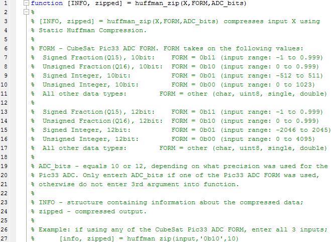
87 huffman_zip function 78

88 79

89 80

90 81

91 huffman_unzip function 82

92 83

93 Appendix B: MATLAB Code for Adaptive Huffman Compression adap_huff_get_codewords function 84

94 85

95 adaptive_huffman_zip function 86

96 87

97 88

98 89

99 adaptive_huffman_unzip function 90

100 91

101 92

102 93

103 Appendix C: MATLAB Code for Static Arithmetic Coding get_freq_arith function arithmetic_zip function 94

104 95

105 96

106 97

107 arithmetic_unzip function 98

108 99

109 100

110 Appendix D: MATLAB Code for Adaptive Arithmetic Coding adaptive_arithmetic_zip function 101

111 102

112 103

113 adaptive_arithmetic_unzip function 104

114 105

115 Appendix E: MATLAB Code for 10 bit Conversion conversion_input_10bit function 106

116 107

117 108

118 conversion_output_10bit function 109

119 110

120 111

121 Appendix F: MATLAB Code for 12 bit Conversion conversion_input_12bit function 112

122 113

123 114