Navigarea Autonomă utilizând Codarea Video Distribuită Free Navigation with Distributed Video Coding (DVC)

Transcription

1 University Politehnica of Bucharest Faculty of Electronics, Telecommunications and Information Technology Navigarea Autonomă utilizând Codarea Video Distribuită Free Navigation with Distributed Video Coding (DVC) Dissertation Thesis submitted in partial fulfillment of the requirements for the Degree of Master of Science in the domain Telecommunications, study program Services and Networks Management Thesis Advisors Student Prof. PhD. Corneliu BURILEANU Elena-Diana ȘANDRU Assoc. Prof. PhD. Eduard-Cristian POPOVICI 2016

2

3

4

5

6

7 Copyright 2016, Elena-Diana ȘANDRU All rights reserved. The author hereby grants to UPB permission to reproduce and to distribute publicly paper and electronic copies of this thesis document in whole or in part.

8

9 TABLE of CONTENTS TABLE of CONTENTS... 9 LIST of FIGURES LIST of TABLES LIST of ACRONYMS INTRODUCTION CHAPTER Video Coding and Multi-View Video Basic Concepts of Video Coding H.264/AVC Standard for Video Coding Multi-View Video CHAPTER Distributed Video Coding Distributed Source Coding Slepian-Wolf Theorem Lossless Transmission Wyner-Ziv Theorem Lossy Transmission Distributed Video Coding Architecture PRISM Architecture DISCOVER Architecture... 46

10 2.3 Multi-View Distributed Video Coding CHAPTER Free Navigation with DVC Application Architectural Solution Schema Architectural Solution Parameters fn_dvc Deployment and Implementation Development User Experience CHAPTER Free Navigation with DVC Results and Observations Comparison Applications, Parameters and Metrics DVC H.264/AVC all Intra RD Performance Comparison RD Performance Points of DVC Decoding Strategies for WZ Frames CONCLUSIONS REFERENCES APPENDIX APPENDIX APPENDIX APPENDIX

11 LIST of FIGURES Figure 1.1 Transform Coding (1) Figure 1.2 Chronology of the International Video Coding Standards Figure 1.3 H.264/AVC Encoder Figure 1.4 H.264/AVC Decoder Figure 1.5 Inter Modes for H.264/AVC Figure 1.6 SIMULCAST Coding Structure for 4 Cameras (1) Figure 1.7 Fully Hierarchical Coding Structure for 7 Cameras (1) Figure 1.8 View Progressive Coding Structure for 4 Cameras (1) Figure 2.1 Traditional Coding Architecture Figure 2.2 Distributed Source Coding Architecture Figure 2.3 Admissible Rate Region - Joint Coding Figure 2.4 Admissible Rate Region - Distributed Coding Figure 2.5 Wyner-Ziv Codec Architecture Figure 2.6 PRISM Architecture (Encoder and Decoder) Figure 2.7 DISCOVER codec, based on Stanford architecture (GOP=4) Figure 2.8 MVDVC - Asymmetric Scheme Figure 2.9 MVDVC - Hybrid Scheme Figure 2.10 MVDVC - Symmetric Scheme Figure 3.1 Architectural Solution Figure 3.2 Hybrid Scheme used in Free Navigation with DVC Figure 3.3 DISCOVER Interpolation Method Figure 3.4 H.264/AVC Codec Results Figure 3.5 DVC Decoder in FN_DVC.m Figure 3.6 SI Generation Method Figure 3.7 Raw Videos Creation Figure 3.8 H.264/AVC all Intra Encoding & Decoding Figure 3.9 DVC Encoding Parameters Figure 3.10 DVC Codec - Encoding... 72

12 Figure 3.11 DVC Codec Decoding [1] Figure 3.12 DVC Codec Decoding [2] Figure 4.1 Path 1, Frame 2 Original Figure 4.2 Path 1, Frame 2, KF H.264/AVC all Intra QP= Figure 4.3 Path 1, Frame 2, KF H.264/AVC all Intra QP= Figure 4.4 Rate-Distortion Performance of DVC, for GOP = 2, with respect to H.264/AVC all Intra, for Path 1 (a), Path 2 (b), Path 3 (c), Path 4 (d), Path 5 (e), Path 6 (f), Path 7 (g), Path 8 (h), Path 9 (i), Path 10 (j) Figure 4.5 Rate-Distortion Performance of DVC, for GOP = 2, with respect to H.264/AVC all Intra for Global Average of the 10 Paths Figure 4.6 Rate-Distortion Performance of DVC, for all 10 Paths Figure 4.7 Rate-Distortion Performance of DVC, for all 10 Paths; Zoom In for QP = 37 (a), QP = 32 (b), QP = 27 (c), QP = 22 (d) Figure 4.8 Rate-Distortion Performance of DVC, for the Decoding Strategies (Interpolation Configurations)... 95

13 LIST of TABLES Table 1.1 Intra-16x16 Prediction Modes Table 1.2 Intra-4x4 Prediction Modes Table 3.1 Cameras Positions Table 3.2 Quantization table for WZF Table 4.1 Experimental Paths Table 4.2 Rate-Distortion (RD) Performance Gain of DVC (H.264/AVC all Intra as Reference) for all the 10 Paths (GOP = 2), obtained with Bjontegaard metric Table 4.3 Rate-Distortion (RD) Performances Gain of DVC (H.264/AVC all Intra as Reference) for the Global Average of the 10 Paths (GOP = 2), obtained with Bjontegaard metric Table 4.4 Rate-Distortion (RD) Performances Gain of DVC Paths (6-10 and 2-7), obtained with Bjontegaard metric Table 4.5 Decoding Strategies for WZFs (Interpolation Configurations) Configuration 1: Orange, Configuration 2: Blue, Configuration 3: Green, Configuration 4: Red Table 4.6 Average RD Performance Points (computed per Frame) for WZFs Interpolation Configurations with respect to QP Values Table 4.7 Rate-Distortion (RD) Performances Gain of the 4 Interpolation Configuration (Decoding Strategies) for WZFs, obtained with Bjontegaard metric... 96

14

15 LIST of ACRONYMS A AVC = Advanced Video Coding C CRC = Cyclic Redundancy Check D db = Decibel DCT = Discrete Cosine Transform DISCOVER = DIStributed Coding for Video services DSC = Distributed Source Coding DVC = Distributed Video Coding G

16 GOP = Group Of Pictures H HDTV = High-Definition Television K KF = Key Frame KBPS = Kilobits Per Second L LPDC = Low-Density Parity Check M MAE = Mean Absolute Error MB = MacroBlock MCTI = Motion-Compensated Temporal Interpolation MPEG = Motion Picture Experts Group MSE = Mean Square Error MV-DVC = Multi-View Video DVC MVV = Multi-View Video P PRISM = Power-efficient, Robust, high compression, Syndrom-based Multimedia coding PSNR = Peak Signal-to-Noise Ratio Q QI = Quantization Index QP = Quantization Parameter

17 R R = Reference RD = Rate-Distortion S SI = Side Information V VCEG = Video Coding Experts Group VLC = Variable Length Coder W WZ = Wyner-Ziv WZF = Wyner-Ziv Frame

18

19 INTRODUCTION Our world is constantly changing and evolving and the technological developments are increasing spectacularly. Phrases such as Century of Speed or Information Century are well known nowadays; the reality is that we live in an era in which, at first, man became dependent on machines due to their ability to facilitate work. Currently, the population growth, the need for communication, globalization, scientific developments have led this man dependency on technology to another level. The challenge of having a society life, rest periods or the help needed with daily chores, pushed technology as indispensable in daily life. Soon, the lack of time has become a major problem, together with the human convenience, so they tried to simplify interaction with machines, to make it faster and easier. The first important achievement was the telephony; fixed and after that mobile. The ability to talk to anyone located anywhere in the world and to be permanently connected was a huge step of evolution. At the same time, man is regarded as a social being, a being who likes to be surrounded by other people, to be able to interact with them, at last virtually if not physically. So did the idea of integrated video feature appear; nowadays, this feature is available on more and more devices. Smartphones, tablets, smart TV, laptops and PCs, airplanes, cars are now equipped with the video feature. Living in the Century of Speed has its disadvantages; most of the time, people complain about the lack of time. Automatically, everyone tries to make up for this by using the time spent between work and home talking to loved ones, watching their favorite show. So, the development of certain methods to enhance the quality of video feature was the next step of technological evolution. Most of them have been focused on video compression. 19

20 In recent years, the improvements in video compression and transmission technologies are increasingly pushing towards a new paradigm called immersive communication, where users have the impression of being present at a real event. Immersive communication includes free-view point video, holography, 3D video and immersive teleconference. The goal of these applications is to offer to users a more realistic experience than the traditional video (where viewers have only a passive way to observe the scene) (1). Over the last one and a half decades, digital video compression technologies have become an integral part of the way we create, communicate, and consume visual information. The Rate- Distortion performance of modern video compression schemes is the result of an interaction between motion representation techniques, intra-picture prediction techniques, waveform coding of differences, and waveform coding of various refreshed regions (2). The basic communication problem may be posed as conveying source data with the highest fidelity possible within an available bit rate, or it may be posed as conveying the source data using the lowest bit rate possible while maintaining a specified reproduction fidelity. In the end, everything is about video compression; but a new concept began to attract the attention of specialists in the field, namely free navigation inside multi-view sequence videos. Since 2002, Distributed Video Coding has become a major paradigm, because of its attractive theoretical results, and its promising target applications (3). Classical video encoding systems imply complex encoders, due to motion estimation and very simple decoders. But DVC can be summed up as coding of multiple correlated sources by separated encoders, while the decoding is computed by a joint decoded. From its many advantages, one can mention that such a compression system implies a complexity reduction of the encoder and also, in the case of multi-view compression, an independent encoding. Thus, combining two important technological trends nowadays, namely the Distributed Video Coding and Free Navigation inside multi-view sequence videos, is the strongest motivation for choosing the theme of this thesis. Following the observations made above, the main objective of this thesis is designing and implementing the MATLAB solution for the Free Navigation with DVC, in order to analyze Distributed Video Coding (DVC) performances compared to H.264 Advanced Video Coding (MPEG-4 AVC) performances, in the case of free navigation inside multi-view sequence videos. In order to do this, a number of specific objectives were considered: Theoretical study of the DVC and H.264 concepts and working principles; Understanding the existing MATLAB scripts, implemented for the two video compression techniques (by the TSI Department from Telecom ParisTech) and performing their customization for the proposed solution; Designing the software solution of Free Navigation with DVC and deciding its parameters (such as number of frames of the video, the path between multi-view sequence); Developing the MATLAB script for the proposed solution; 20

21 Drawing the conclusions based on the RD (Rate-Distortion) performances of DVC with respect to H.264/AVC all Intra and choosing the best suitable solution for Free Navigation concept; Deciding the best decoding strategy (interpolation configurations) of WZ frames for the chosen scenario, in terms of RD performances. This thesis is structured in four chapters; first two show the theoretical aspects of video coding and Multi-View videos, along with the main characteristics and architectural aspects of DVC and H.264/AVC all Intra. The last two chapters reveal the author's contribution to the development of the practical part of this thesis. The personal contribution can be summarized as follows: Creating an achievable architectural solution for the main objective; Designing and implementing the MATLAB application (FN_DVC.m), application simulating the Free Navigation concept for a given path and obtaining the Rate- Distortion performance points for each frame of the path, for both video coding standards (DVC and H.264/AVC all Intra); Deciding the set of parameters for the proposed scenario (values of the quantization parameters and indexes [ ] and [ ], parameters of encoding and decoding for H.264/AVC all Intra and DVC); Establishing the path configuration for the 10 paths used for the experiments; Choosing the SI generation method and the multi-view scheme (Hybrid), along to the decoding strategies and narrowing their number to four; Customizing the function decodwzf to fit the solution; this implied changing the set of the codec parameters in order to implement the function linking QI and QP; Obtaining the RD performance points for both coding strategies; the rate and the PSNR per each frame (Intra and KF/WZF) as a function of QP; Deciding the entities of the RD performance comparison; DVC H.264/AVC all Intra (each path individually, global average of 10 paths) and DVC (all 10 paths, interpolation configurations); Choosing the Bjontegaard metric and the RD curves as a basis for the comparison; Designing and implementing MATLAB scripts (allintra-dvc_comparison.m and Global_and_All_Comparison.m), in order to obtain the comparison results by processing the RD performance points obtained from FN_DVC.m for both coding strategies; the rate and the PSNR per each frame (Intra and KF/WZF) as a function of QP; Drawing the conclusions and observations; deciding if Free Navigation with DVC is a suitable solution (if its RD points outperforms H.264/AVC all Intra) and which decoding strategy for WZ frames is better (from the four interpolation configurations). The thesis was realized in cooperation with the University TELECOM ParisTech (F PARIS083), from Paris, France, under the guidance of Prof. PhD. Beatrice PESQUET-POPESCU and Prof. PhD. Marco CAGNAZZO, during an ERASMUS+ placement, between 25th of March and 24th of June 2016, identified by 2275/

22 22

23 1. CHAPTER 1 Video Coding and Multi-View Video Videos are three-dimensional signals I k (m, n): the pair (m, n) defines the space, while k the time. Referring to digital videos, the three variables m, n and k are discrete. Each image I k (m, n) is called frame and f frames per second are displayed for giving the illusion of fluid movement. The parameter f is called frame rate. Video signals require a large amount of data to be stored and transmitted. The goal of video compression is to reduce the size of the video file, with an acceptable loss in quality. Traditional video coding techniques focus on eliminating the redundant elements of the signal (psychophysical and statistical). (4) The main property of the video signals is the large correlation in time and in space. For several decades, video compression has been the research topic aimed to mobilize many researchers, along with industrial partners. If its main goal was only reducing the rate necessary for the descriptions of the video sequence, as years passed by the compromise between a lower rate and high decoded quality became more present and all new paradigms are aimed to improve this compromise. In recent years, the improvements in video compression and transmission technologies increased; in this way, immersive communication appeared. This paradigm refers to the users feeling as being present at a real event. Immersive communication includes free-view point video, 23

24 holography, 3D video and immersive teleconference. The goal of these applications is to offer to users a realistic experience than the traditional video (where viewers have only a passive way to observe the scene). In this chapter, the basic concepts of predictive video coding are reviewed along with the date compression standard, H.264/AVC, which will serve as basis for comparison in this thesis. Moreover, Multi-View video is presented and the most common compression architectures are described. 24

25 1.1 Basic Concepts of Video Coding Studies has shown that the human visual system can form, transmit and analyze somewhere between 10 and 12 images per second and perceive them individually. This represents the principle of the video sequence representation; this is due to the continuity illusion created when more than 12 images per second are submitted to the human visual system. As already stated, videos are three-dimensional signals I k (m, n): the pair (m, n) defines the space, while k the time. Referring to digital videos, the three variables m, n and k are discrete. Each image I k (m, n) is called frame and frames per second are displayed for giving the illusion of fluid movement. The parameter f is called frame rate. Due to the above statement, the frame rate is between 15 and 30 frames per second, in order to represent a visual scene by a digital video sequence. There are situations when the frame rate is 60. Digital videos are characterized by redundancy and digital coding tries to minimize it in each domain (time and space). Unfortunately, coding and compression lead to distortions of the video, so it is a matter of choice between the total bit rate R used for coding the video and the distortion D between the coded and the original frames. As it can be easily intuited, the distortion should be minimized, while the total bit rate should be constant. Therefore, the cost function is: where λ is a Lagrangian multiplier. J = D + λ*r (1.1) Typically, for images, the coding rate R can be defined in bits per pixel R b/p = B N M (1.2) where B represents the numbers of bit used for compressing the video and M * N represents the spatial resolution of the video. In order to convert it in bits per second, the following multiplication is done: R b/s = R b/p N M f (1.3) Let us consider I the original image and I the decoded image. The distortion between these two images can be measured with an objective metric. Popular objective metrics are the Mean Square Error (MSE) and the Mean Absolute Error (MAE), but the most conclusive on is the Peak Signal-to-Noise Ratio (PSNR), defined as: PSNR = log (2 b 1) 2 1 M N N m 1 M n=1 I k (m,n) I k(m,n) 2 (1.4) where (2 b 1) 2 is the maximum possible pixel value (usually b = 8). 25

26 Although desired, lossless compression is not very efficient because it provides a moderate amount of compression. On the other hand, lossy compression is necessary in order to obtain a lower rate and a fair distortion. Spatial correlation is used in image coding in order to reduce the size of that image. The spatial correlation represents the correlation among neighboring samples (5). The most used method of spatial compression in image and video coding is Direct Cosine Transform (DCT). Temporal correlation is the correlation among successive frames of a video sequence. In almost all the cases, in a video sequence one can exploit both types of correlation. In order to optimize the Rate-Distortion performance, each frame is compressed at a time, as shown in Figure 1. It is composed of a cascade of transform, quantization and variable length coder (VLC). The first step is to explore the correlation, then to educes the total bit rate and in the end, lossless coding performed by the VLC eliminates other statistical redundancies. Transform Quantization VLC Figure 1.1 Transform Coding (1) The coding is performed in the transform domain because it allows the decorrelation, both spatial and temporal, permitting a more compact parametric representation of the information. The main advantages of the DCT are: for real signal, DCT image is also real; it presents a high degree of compactness. 26

27 1.2 H.264/AVC Standard for Video Coding Video coding standards are developed by two important groups, namely MPEG Moving Image Experts Group and VCEG Video Coding Expert Group. As the topic of this thesis is video coding, in Figure 2 it can observed the chronology of the international video coding standards. MPEG developed MPEG-1 and two MPEG-2 and MPEG-4 standards for coding video and audio. MPEG-2 and MPEG-4 are commonly used for transmission and storage of video sequences. H.261 was the first video telephony standard and H.263 was its successor; both of them were standardized by VCEG (6). The joint of these two groups created H.264/AVC (also referred as H.264/MPEG-4 AVC). Figure 1.2 Chronology of the International Video Coding Standards H.264/AVC represents one of the most common standards for video coding. Obviously, H.264/AVC contains an important part of the basic modules that can be found in its predecessors (MPEG-1-4 or other H.26x), such as: transform, prediction, quantization. Moreover, the standardization team took those modules and enhanced them as follows. Figure 1.3 describes the architecture of a H.264/AVC Encoder. The first characteristic is the fact that all the frames are divided into two categories: Intra-Frames and Inter-Frames. Firstly, in Intra-coding mode, the encoder exploits only the spatial correlation, by estimating a good prediction of the sample based on neighboring samples. Secondly, Inter-coding mode is characterized by 27

28 exploiting the temporal correlation as well; inter-frames temporal prediction, such as motion compensation using already decoded frames. Essentially, the encoder tries to estimate motion vectors and to identify the reference frame which will help predict the samples of the frame to be coded. In either way, a residual prediction is computed as the difference between the original frame and the predicted frame. This residual is further transformed in order to obtain the transform coefficients that are quantized and in the end entropy encoded. Figure 1.3 H.264/AVC Encoder The architecture of the H.264/AVC Decoder can be observed in Figure 1.4. It can be easily observed that the encoder and the decoder have common parts; since the encoder estimates the same prediction as in the decoder, its architecture includes also a part of the decoder. In this way, the encoder and the decoder have the same prediction for the samples. The decoding flow is the following one: the quantized coefficients are first inversed scaled, followed by an inverse transform; these operations try to reconstruct the residual. Then, the prediction process is performed (using the motion compensation) and in the end, the approximated residual is added to the predicted samples, and filtered by a deblocking filter. In H.264/AVC the color space is YCbCr; its advantage is the following one: by separating the luma information from the chroma information, the luma can be stored at high resolution, while the chroma can be stored at low resolution. Y represents the brightness and is called luma, while Cb and Cr are chroma components: blue-difference and red-difference. This separation is performed because the human eye is more sensitive to luma than to chroma. 28

29 Figure 1.4 H.264/AVC Decoder The subjective correlation of the chroma components can be reduced using the subsampling (or decimation) of these components with respect to luma. Considering the notation Y:Cb:Cr, H.264/AVC typically uses 4:2:0 sampling (the chroma component has one fourth the number of samples of the luma component (5)). A. Division of a Frame Each frame of a video sequence is structured into small divisions called macroblocks (MB), areas of 16x16 samples of luma component and 8x8 samples of the difference chroma components. The samples of a MB can be spatially or temporally predicted; the resulting residual in divided into blocks, integer transformed, quantized and entropy coded. Further, macroblocks are grouped in slices (group of successive MBs). There are five possible slide-coding types, as follows: I slice: only Intra-prediction is possible; it contains intra-coded MBs predicted from previously decoded samples of the same slice; P slice: Skip, Intra-prediction and Inter-prediction is possible; it can contain intercoded MBs predicted from previously decoded samples of other frames, intra-coded MBs or even skipped MBs; B slice: prediction from future slices and from average of past and future slices is possible; it contains inter-coded MBs predicted from previous decoded frames and future slices; Switching I slice: specific for efficient switching between bit-streams coded at various bit rates; Switching P slice: specific for efficient switching between bit-streams coded at various bit rates (5). Moreover, each MB from a slide can be coded as: Skip mode no information is sent for that particular MB; 29

30 Intra mode used for spatial prediction; Inter mode used for temporal prediction; Direct mode the particular MB is coded in the same way (using the same motion vectors) the previous MB was coded. Obviously, each mode generates a different number of coded bits and also a different distortion. If Rate-Distortion optimization is performed, the goal of the encoder is to minimize the decoded distortion D and to minimize the bit rate R. The encoder searches for the mode that minimizes the function J = D + λr. Large values of λ tends to give more emphasis to the rate than to the distortion. In literature, an optimal value for λ depending on the quantization parameter (QP) has been obtained empirically as (1) λ = 0.852(QP 12) 3 (1.5) B. Spatial Prediction (Intra) The spatial prediction is possible for I-slices. The predicted samples of a block are formed from the neighboring previously encoded and reconstructed samples, leading to Intra-prediction. There are two types of intra coding (7): Intra and Intra-4 4. Intra-16x16 is used for smooth image areas; actually, uniform prediction is performed for all the MBs. Intra_16x16 mode involves 2 blocks: 16x16 luma block used for coding smooth areas of a picture and 8x8 chroma block. Intra-16x16 has four prediction modes, as they are listed in Table 1.1: PREDICTION MODE Vertical Prediction Mode 0 Horizontal Prediction Mode 1 DC Prediction Mode 2 Plane Prediction Mode 3 DETAILS Involves extrapolation from upper samples Involves extrapolation from left samples A mix between modes 0 and 1; it implies the mean of upper and left-hand samples (8) A linear plane function is fitted to the upper and left-hand samples Table 1.1 Intra-16x16 Prediction Modes 30

31 Intra-4x4 is used for picture parts rich in details; each 4x4 block is predicted from spatially neighboring samples. Intra-4x4 has nine prediction modes, as they are listed in Table 1.2: PREDICTION MODE Vertical Prediction Mode 0 Horizontal Prediction Mode 1 DC Prediction Mode 2 Diagonal Down-Left Prediction Mode 3 Diagonal Down-Right Prediction Mode 4 Vertical-Left Prediction Mode 5 Horizontal-Down Prediction Mode 6 Vertical-Right Prediction Mode 7 Horizontal-Up Prediction Mode 8 DETAILS Involves extrapolating vertically the upper samples Involves extrapolating horizontally the left samples A mix between modes 0 and 1; it implies the mean of upper and left-hand samples (8) The samples are interpolated at 45 angle between lower-left and upper-right The samples are interpolated at 45 angle down and to the right Involves extrapolation at an angle approximatively 26.6 to the left of vertical Involves extrapolation at an angle approximatively 26.6 below horizontal Involves extrapolation or interpolation at an angle of approximatively 26.6 to the right of vertical Involves interpolation at an angle of approximatively 26.6 above horizontal Table 1.2 Intra-4x4 Prediction Modes C. Motion-Compensated Prediction (Inter) The temporal correlation between the frames is exploited by Inter-prediction modes. The prediction is estimates based on several previously encoded and decoded frames. They are supported by P and B-slices. As already stated, while for P-slices, only prediction using past frames is possible, for B-slices also prediction using future slices can be considered. Figure 1.5 displays the types of inter coding in H.264/AVC, which offers more flexible block partition, multiple references and also Enhanced Direct and Skip Macroblock modes: 31

32 16x16 16x8 8*16 8x8 8x4 4x8 4x4 Figure 1.5 Inter Modes for H.264/AVC Inter-16x16 Inter-16x8 Inter-8x16 Inter-8x8 If Inter-8 8 mode is chosen, an additional syntax element for each 8 8 macroblocks is used to specify if it is partitioned in 8 8, 8 4, 4 8, 4 4 blocks: Inter-8x4 Inter-4x8 Inter-4x4 The motion compensation is performed at a resolution of up to 1 4 pixel. Pixels at quarterpixel position are computed using bilinear interpolation. Regarding multiple references, multi-picture motion-compensated prediction is also possible; each MB of the P-slices can be estimated from one, more different reference frame or from a weighted sum of a series of reference frames. This new improvement allows pictures of better quality in scenes where there are changes of plane or zoom. As for the Direct and Skip modes, they are very frequently used, especially with B-frames. The first mode, Direct mode consists in choosing, for the current MBs, the previously MBs syntax elements (mode and vector). The Skip mode is possible for both P and B slices: the MB is coded without sending residual error or motion vectors. The prediction is the co-located block in the reference frame: spatial and temporal. 32

33 D. Transformation & Quantization This standard can use three transforms; the choice is done based on the residual data, as it follows: Hadamart transform for 4x4 array of luma DC coefficients in Intra MB (16x16 mode) H 4x4 = ( ) (1.6) Hadamart transform for 2x2 array of chroma DC coefficients in Intra MB (16x16 mode) H 2x2 = ( ) (1.7) Integer DCT transform for all 4x4 arrays of the residual data H DCT = ( ) (1.8) In H.264/AVC there are 52 values for QP; after the transform, the coefficients are scaled and after that quantized based on the value of QP. The resulting coefficients are scanned in a zig-zag manner and entropy encoded. 33

34 1.3 Multi-View Video For decades now, the video compression is a spread subject in the research circles. Moreover, the transmission technologies have experienced a rapid growth. This joint increase has given rise to a new paradigm the immersive communication. Immersive communication gives the users the impression of being present at a real event, including a vast series of applications: free-view point video, holography, 3D video and also immersive teleconference; these applications are aimed to offer a realistic experience compared to the traditional video, thus increasing the user experience. In order to deliver a more realistic feeling to the user, he/she should benefit from a broad perspective of the scene. In order to obtain this, one may use Multi-View Video (MVV). MVV consists of a series of N cameras filming the same scene from different angles; the cameras used to record the scene are arranged in different spatial positions, obtaining a set of N 2D videos, namely multi-view videos. Nevertheless, when using N cameras to film the same scene, the required storage increases proportionally with N. But due to better compression algorithms and a high redundancy in time, view and spatial domain, the amount of data to be stored is kept under normal values. The compression techniques used in H.264/AVC represents the starting point for techniques aimed for multi-view videos: SIMULCAST: each view is coded independently (9). In figure 1.6 it can be seen an example of SIMULCAST coding structure for four cameras and a GOP equal to 8. The advantage of SIMULCAST, from computational point of view, it is a simple structure which performs only temporal prediction and gives random access to each view, at any time. The main disadvantage is linked to the inter-view correlation that is not exploited at all, thus the storage needed is still increased. Figure 1.6 SIMULCAST Coding Structure for 4 Cameras (1) 34

35 H.264/AVC Standard Extensions: derived from H.264/AVC and customized for Multi-View Video coding. There are 2 possible schemes: Fully Hierarchical: figure 1.7 displays an architecture of fully hierarchical coding structure for seven cameras and a GOP equal to 8. This scheme exploits both temporal and inter-view correlation for P and B frames (except the frames of the first view, called base view, still coded independently). The main disadvantage consists in the impossibility of having random access without decoding the entire GOP. Figure 1.7 Fully Hierarchical Coding Structure for 7 Cameras (1) View Progressive: represents a trade-off between the other 2 possible schemes. As in Fully Hierarchical, the first view is coded independently. The inter-view correlation is exploited along the view axis (for the frames called I-frames); the other frames (called V-frames) are predicted from the I-frames. In the case of P-frames, only the temporal correlation is exploited. In this case, the random access is possible: P-frames can be easily decoded (as in SIMULCAST architecture), while for the key frames, the reference frames must be firstly decoded. In figure 1.8 can be depicted the scheme for four cameras and a GOP size of 8. 35

36 Figure 1.8 View Progressive Coding Structure for 4 Cameras (1) 36

37 2. CHAPTER 2 Distributed Video Coding Distributed Video Coding is a relatively new paradigm based on two fundamental theorems: Slepian-Wolf (in case of lossless compression) and Wyner-Zig (in case of lossy compression); as a matter of fact, DVC is originated in Distributed Source Coding, an important part of information technology, dealing with the compression of multiple information sources, correlated but not linked one to another (they do not communicate with each other). By exploiting the correlation between the sources, the advantages are remarkable. DSC exploits the correlation between the multiple sources at the decoder side (together with channel codes) and in this way the computational complexity characterizing the encoder is shifted at the decoder. This highlights also one of the first important advantage of DVC, compared to the traditional video coding: the computational burden in encoders is shifted to the joint decoder, leaving a very low complexity encoder to perform the compression of the videos. DVC, as inherited from DSC, is based on encoding separately the correlated frames and decode them jointly. This architecture suits both Mono-View and Multi-View video systems, obtaining (in theory) the same performances as in traditional video coding. 37

38 In this chapter, the basic concepts and origins of DSC are reviewed along with the architectures implemented for Distributed Video Coding, in the case of Mono-View videos, but also the customization made for Multi-View videos. 38

39 2.1 Distributed Source Coding Distributed Source Coding represents an important problem of information technology; it focuses on coding multiple video sources, correlated, in a distributed manner. Each signal is encoded by a different encoder and the streams of bits are sent to a single, joint decoder, which will exploit the correlation between the frames by performing a single decoding. As first Shannon Theorem states: given a source X, modeled as a discrete random variable with entropy H(X), it can be encoded and decoded without any loss of information if encoding rate is greater than or equal to its entropy. Let us consider two discrete sources: X and Y. For a lossless coding, when X and Y are independently coded, the encoding rate must be greater or equal to their entropy, as it can be seen in the following equation: R X H(X) (2.1) R Y H(Y) (2.2) These two sources can be encoded and decoded jointly without any loss of information if the total encoding rate is greater or equal to their joint entropy H(X, Y), as in equation 2.3: Their joint entropy is defined as: R H(X, Y) (2.3) H(X, Y) = x χ y Υ f XY (x, y) log 2 (f XY (x, y)) (2.4), where f XY (x, y) represents the joint probability density function of X and Y. Also: H(X) + H(Y) H(X, Y) (2.5) Figure 2.1 depicts the traditional coding scheme, for jointly encoding and decoding; as already stated, for no loss of information, the encoding rate must be greater or equal to the joint entropy. Figure 2.1 Traditional Coding Architecture 39

40 Figure 2.2 shows the DSC paradigm; must be highlighted the fact that the two sources are correlated. In DSC, the encoding is performed independently on both sources and the decoding in jointly implemented in the decoder. Figure 2.2 Distributed Source Coding Architecture But due to Shannon Theorem, if X and Y are separately encoded, they can also be decoded without any loss of information if: R X + R Y H(X) + H(Y) (2.6) Slepian-Wolf Theorem Lossless Transmission The Slepian-Wolf Theorem states that (1): For the distributed source coding problem of the pair (X, Y) with joint probability mass function f XY (x, y), the achievable rate region (with no errors) is given by the following equations: R X H(X Y) (2.7) R Y H(Y X) (2.8) R X + R Y H(X) + H(Y), where H(X Y) is the entropy of X when Y is known. In figure 2.3 can be seen the representation of the admissible rate region in the case of joint encoding and decoding, in terms of encoding rates of the two sources. Figure 2.4 shows the admissible rate region for DSC; it can be concluded that this region is larger than the rate region for separately encoding and decoding of the two variables (grey area), but still smaller than the region obtained for joint coding (as shown in figure 2.3). 40

41 Figure 2.3 Admissible Rate Region - Joint Coding Figure 2.4 Admissible Rate Region - Distributed Coding Either way, Slepian and Wolf stated that from rate performance point of view, encoding correlated sources jointly or independently, while the decoding is performed with a known correlation model, the process is still with no loss of information. 41

42 2.1.2 Wyner-Ziv Theorem Lossy Transmission The Slepian-Wolf Theorem concerns only the case of lossless coding; Wyner and Ziv took further this paradigm and extended it for the lossy case, when some information loss can be allowed. Wyner and Ziv introduced the Rate-Distortion. Figure 2.5 illustrates the basic Wyner-Ziv codec architecture. As it can be seen, the source X overcomes a set of steps: transformation, quantization and encoding (using a Slepian-Wolf encoder). At the decoding side, the stream of bits is decoded (using a Slepian-Wolf decoder), the reconstruction is performed and then the inverse transform. As it can be easily observed, in order to obtain the reconstructed image X, the Side Information (SI) is estimated. Figure 2.5 Wyner-Ziv Codec Architecture In the case of two correlated sources, the statistical dependence between X and Y is modelled as a virtual correlation channel, and Y is considered as a noisy version of X (10). The encoder computes the parity bits for X and sends them to the decoder. The decoder estimates X given the received parity bits and the side information Y regarded as a noisy version of the code-word systematic bits. Let us consider D = E[d(X, X )] - the maximum distortion accepted at the decoder and R X Y (D) - the admissible rate with distributed coding while R X Y (D) - the admissible rate for classical joint coding (when the side information Y is available at the encoder) and R X (D) - the admissible rate for encoding X without SI, at distortion D (1). So: R X Y (D) R X Y (D) R X (D) (2.9) The Wyner-Ziv Theorem states that if D is the MSE error and X and Y are joint Gaussian variables, then R X Y (D) = R X Y (D) (2.10), where the distortion is equal to D = E[ X X 2 ] (2.11). 42

43 In conclusion, Wyner and Ziv proved that the same rate cam be achieved for the systems that exploit the correlation (statistical dependency) between the sources at the decoding side, as well as for the ones exploiting at the encoding side (for jointly Gaussian sources and for a mean square error distortion). 43

44 2.2 Distributed Video Coding Architecture DVC can be summarized as a new paradigm characterized by the movement of the computational complexity from the encoding side to the decoding side, as the work of both teams (Slepian-Wolf and Wyner-Ziv) proved: under some certain conditions, the correlation between the sources (and implicitly between the successive frames of the video) can be exploited at the joint decoder without any loss in performance, with an important gain in the encoder complexity. Based on the theories of Slepian-Wolf and Wyner-Ziv, to different approaches have been proposed: PRISM architecture and Stanford-DISCOVER architecture PRISM Architecture The PRISM architecture, or Power-efficient, Robust, high compression, Syndrom-based Multimedia coding (11) represents one of the first architectural implementation of the Wyner-Ziv coding. Several evolved versions have been implemented since then and figure 2.6 displays the version presented in Figure 2.6 PRISM Architecture (Encoder and Decoder) 44

45 ENCODER: PRISM has block-based architecture, each frame of the video is divided into 8x8 blocks. Each block is further processed as in figure 2.6. Transform the block is transformed using DCT; the resulting coefficients are arranged in one-dimension vectors (64 coefficients) by performing a zig-zag scan on the two-dimension block (8x8); Quantization the resulted coefficients are quantized with a given quantization step, dictated by the quality wanted at the reconstructions; Classification the most important step of this architecture. During it, the correlation between the source and the SI is exploited, in order to classify the blocks and moreover the bit planes, into three distinct categories: Skipped bit plane, WZ encoding and Entropy encoding. The reference block is actually the SI and it can be computed differently (it depends on the computational capability of the encoder): for low power encoders SI is the previous block and there no motion search; for powerful encoders SI is the most similar block to the current one, found in the previous frame by running complex motion search algorithms. After finding SI, the correlation between the source coefficients (64) and the SI coefficients (64) helps finding which bit planes are worth inherited from the SI, in this way they will not be send to the decoder because can be easily recovered from the SI. The rest of bit planes (that cannot be recovered at the decoder) are split into two categories: the most significant are WZ encoded and the least significant are entropy encoded; Syndrome Encoding the output of the classification block is either a WZ encoded bit planes or an entropy encoded bit planes. For the first type, the arity check matrix of a linear correction code is used; Hash Generator in order to easily predict at the decoder, a CRC of 16 bits is generated at the encoder, being used as a signature of the quantized codeword sequence. DECODER: after being encoded, the 8x8 blocks are decoded using the modules depicted in the scheme from figure 2.6: SI Generation first of all, the decoder tries to find the best prediction of the current block, by performing a motion search and generating a set of possible matches. The received syndrome is being decoded with each possible match and the selected SI is the one match that satisfies the hash check module; Syndrome Decoding is divided into two steps: firstly, the encoded bit planes (both WZ and entropy) are decoded; secondly, the closest code-word to the SI is found (within a specified coset); Hash Check the checksum of the previously decoded block is computed and compared to the one transmitted from the encoder; if the two variables match, the decoding is successful; if not, the decoding restarts with another possible match; 45

46 Estimation and Reconstruction at this point, the recovered quantized codeword sequence and the predictor are used to reconstruct the source, based on the mean square error; Inverse Transform an inverse zig-zag operation is performed on the reconstructed coefficients to obtain the 2-D block, which will be passed through an inverse transform and the pixels are obtained DISCOVER Architecture In the same time PRISM was presented (2002), a group of scientists from Stanford proposed another architecture implementation for the Wyner-Ziv coding; the differences between the two proposed models was the approach: while PRISM was a block-based architecture, the new solution was characterized by a frame approach. The video sequences consist of two types of frames: Wyner- Ziv frames (WZF) and Key frames (KF); moreover, the frames are encoded separately and also differently based on the type. The KFs are Intra coded and the WZFs are DCT transformed, quantized and fed into a systematic channel encoder. The most known architecture and the reference method for DVC was developed during the European project DISCOVER (DIStributed Coding for Video services) (12). For DISCOVER, a GOP of size n consists of 1 KF and n-1 WZFs. Figure 2.7 depicts the DISCOVER codec, based on Stanford architecture for a GOP equal to 4. Figure 2.7 DISCOVER codec, based on Stanford architecture (GOP=4) 46

47 ENCODER: As it can be observed in the scheme, the DISCOVER encoder divided into two parts, after the splitting of the frames. Firstly, the KFs are encoded using and intra frame coder H.264/AVC Intra Encoder. The upper part of the architecture concerns WZFs. Image Classification the frames of the sequence to be encoded are divided into two types: WZFs and KFs. The size of the GOP is fixed and it an important player for the WZF estimation quality; a smaller GOP will dictate a better quality, while a greater GOP implies a complexity decrease (because KFs are more complex than the WZFs); Transform and Quantization the WZF is transformed using a 4x4 DCT and the 16 resulting coefficients are organized in 16 bands b k, k [1, 16]. The low frequency coefficients (DC coefficients) are positioned in the first band and the others are grouped in the AC bands k [2, 16]. The next step represents the quantization: each band of DCT coefficients is quantized with 2 m k levels. The number of reserved bits m k depends on the band k. In DISCOVER, the number of levels is given by 8 already determined Quantization Indexes (QI); QI=1 corresponds to a low bit rate, while QI=8 corresponds to a high bit rate. Also, QI is linked to the QP used for encoding the KFs. Channel Encoder the quantized symbols resulted after the previous steps (for each DCT band) are divided into bit planes, obtaining two types of data: the systematic data and the parity data. At the beginning, the role of the channel encoder of producing parity bits was aimed to correct (if any) the errors found on the systematic bits, at the decoder. But in DVC, the role of the channel encoder is different: the systematic information is no longer transmitted to the decoder, but replaced by the SI; only a part of the parity bits is transmitted to the decoder and this time in order to correct the SI errors. The process is the following: each bit plane is fed into the channel encoder and the set of the parity bits is computed (and the systematic bit are discarded). Afterwards, the parity information is stored into a buffer and send to the decoder, when requested by it through the feedback channel (bit error rate at the decoder exceeds a certain threshold). There are two possible design solutions for the codes: LPDC coder or turbo codes. In a turbo code architecture, the bit stream and an interleaved version of it are fed separately into two convolutional channel encoder. The systematic parts are discarded and the two sets of parity bits are sent to the decoder. Also in this case, only a punctured version of the parity bits is initially sent to the decoder according to the minimum rate estimation. Then, if necessary, more bits will be sent (1). DECODER: The KFs are directly decoded with the H.264/AVC Intra Decoder and then are being used to generate the SI needed for WZF decoding process. Side Information Generation the quality of the SI is directly related to the performances of the DVC. Firstly, the decoder must find a prediction for the WZ frame; secondly, this estimation will be corrected by the parity bits sent by the encoder. There are two types of methods for building the SI: 47

48 interpolation and extrapolation. The SI interpolation is performed by considering past and future frames, while extrapolation considers only past frames. One of the most common algorithms is DISCOVER motion temporal interpolation algorithm (MCTI); it consists of the following steps: o Low-Pass Filtering of the reference frames in order to improve the motion vectors reliability; o Forward Motion Estimation between the previous and the next frames; o Bidirectional Motion Estimation in order to refine the motion vectors; o Spatial Smoothing of Motion Vectors aimed to obtain a higher value for the field spatial coherence and reduce the number of false motion vectors; o Bidirectional Motion Compensation in order to avoid spatial incoherence. Channel Decoder Let us denote the side information by Y; it is considered a noisy version of the original WZF, X. The noise is additive, so Y = X + N, where N is the noise. In order to obtain the DCT coefficients (seen as the noisy version of the WZF DCT coefficients), the generated SI is transformed, using a 4x4 DCT block. When the SI DCT coefficients are known, the decoder (Slepian-Wolf) starts correcting the bit errors by using the parity bits from the encoder (requesting them through the feedback channel). After decoding each packet of bits, the error is computed by the decoder; it is greater than the threshold (10 3 for DISCOVER), more parity bits are required. Reconstruction and Inverse Transform The reconstruction is performed using SI DCT coefficients and the decoded DCT coefficients. In the end, the inverse 4x4 DCT transform is performed and the frame is restored in pixel domain. DVC is particularized by a certain element in its architecture, namely the feedback (or backward) channel. Unfortunately, is represents also an important drawback of the solution; because the encoder needs to wait in order to send all the parity bits to the decoder, DVC Stanford architecture is actually a real-time decoding paradigm. During the years, several solutions without this looped have been presented. While the advantages are obviously, the disadvantages are the following: losses in performance (around 1dB) and also a not very complex comparison between the KFs (previous and next), in order to have a measure of the correlation. 48

49 2.3 Multi-View Distributed Video Coding Multi-View Distributed Video Coding (MVDVC) or Stereo DVC represents a paradigm similar to Mono-View DVC, is the sense of the encoding and decoding processes involved. Moreover, there are some differences between the two paradigms: SI generation and frame distribution (based on time) in the time-view space. One of the major disadvantage of the traditional multi-view coding is the necessity of intercamera communications in order to be able to exploit the inter-view redundancies. For this, the complexity of the encoder is increased, because it has to be able to perform inter-view redundancies exploitation and complex motion estimation based for intra-view. But MVDVC can minimize both of these encoder complexities. In MVDVC, for a frame reference there are two indexes needed, one for the time and one for the view. Let us denote I t,k, the image taken at the instant t by the k -th camera. The corresponding SI is I t,k. Multi-View Schemes in Mono-View DVC the main issue is deciding the number of WZ frames in a GOP. But in MVDVC, the problem is more complex because of the number of the frame distribution. Although it may appear there are many possible configurations, their number can be reduced. But firstly, in MVDVC systems, there are three types of cameras used: o Key cameras: all the generated frames are KFs, that can be encoded by either an Intra or an Inter coder. Consequently, these cameras are more powerful; o Wyner-Ziv cameras: all the generated frames are WZFs; the SI is build using KFs from another camera. Hence, their complexity is not that high; o Hybrid cameras: the generated frames can be KFs or WZFs. The SI can be computed based on KFs from another cameras or their own KFs. The advantage of this type is the symmetry of the configuration, the disadvantage is the powerful cameras needed. These cameras can be arranged in a variety of configurations. However, there are three main schemes: Asymmetric scheme is characterized by an alternation between the Key and Wyner-Ziv cameras, as it can be observed in figure This type is the least expensive in terms of the needed equipment, because there are dedicated cameras for the two types of views. Hybrid scheme the cameras used are hybrid cameras. At the same time t, all of the cameras will transmit either a Key frame or a Wyner-Ziv frame. It requires complex cameras, able to sustain the computational necessity. The schematic architecture can be depicted in figure 2.17, where can be found five cameras during six moments of time. 49

50 Figure 2.8 MVDVC - Asymmetric Scheme Figure 2.9 MVDVC - Hybrid Scheme Symmetric scheme similar to the Hybrid scheme, this scheme is composed of hybrid cameras. There is one KF for one WZF, meaning the report is ½, and the frames (KFs and WZFs) are placed in a time-view grid. The SI for each WZF can be generated in the view or time direction, as figure 2.18 shows. 50

51 Figure 2.10 MVDVC - Symmetric Scheme SI Generation in Mono-View DVC, the SI generation is not a very complex strategy. But in MVDVC, because of the time-view axes, the complexity increase. According to the arrangement of Key, Wyner-Ziv and Hybrid cameras, the SI for the WZ frames can be estimated in different ways: the temporal estimation: the interpolation is based on temporal adjacent frames of the same view; the inter-view estimation: the interpolation is based on the frames of the adjacent views at the same time instant; a fusion between temporal and inter-view estimations: the temporal and the inter-view estimations are fused according to different criteria (1). A fusion represents the combination used to create a single Side Information, when both temporal and inter-view interpolations are available (as in Symmetric type of scheme). 51

52 52

53 3. CHAPTER 3 Free Navigation with DVC Application Nowadays, a huge number of the world population uses image and video coding technologies on a regular basis (and this percentage is still growing). These technologies are behind the success and quick deployment of services and products such as digital pictures, digital television, DVDs, and Internet video communications (13). Most of the video coding paradigms are characterized by powerful encoders, able to exploit the temporal and spatial correlations between the frames. As a consequence, all standard video encoders have a much higher computational complexity than the decoder (typically five to ten times more complex). But Distributed Video Coding represents a paradigm that moved the computational complexity from the encoder to the decoder, being suited for sensor networks. DVC refers to the compression of correlated signals captured by different sensors that do not communicate between themselves. All the signals captured are compressed independently and transmitted to a central decoder, which has the capability to decode them jointly. In recent years, the improvements in video compression and transmission technologies increased; in this way, immersive communication appeared. This paradigm refers to the users feeling 53

54 as being present at a real event. Immersive communication includes free-view point video, holography, 3D video and immersive teleconference. The goal of these applications is to offer to users a realistic experience than the traditional video (where viewers have only a passive way to observe the scene). Therefore, the concept of Free Navigation inside a multi-view video sequence started attracting more researchers willing to find the suitable video encoding paradigm able to offer a satisfactory user experience at a decent computational power of the architecture. The first plan on which the author of the thesis worked for the practical implementation of the paper was designing and implementing an application able to simulate the concept of Free Navigation and to obtain the RD performance points for both coding strategies: DVC and H.264/AVC all Intra. 54

55 3.1 Architectural Solution Schema The main objective of this thesis is to decide if Free Navigation with MVDVC can be a suitable solution for the immersive communication. In order to deliver a more realistic feeling to the user, he/she should benefit from a broad perspective of the scene. Therefore, Multi-View videos are used. MVV consists of a series of N cameras filming the same scene from different angles; the cameras used to film the scene are arranged in different spatial positions, obtaining a set of N 2D videos, namely multi-view videos. So, the purpose of this paper is developing a software solution which can simulate the situation in which a user can decide what perspective he/she wants to visualize in the watched video at each moment of time, and measure its performances. The first phase in finding the architectural solution is to establish the components of the scheme. In order to decide whether MVDVC is a suitable video coding paradigm for free navigation, in terms of performances, one must decide the reference used for the comparison. As already stated, the performance comparison will be performed in Chapter 4, in order to analyze Distributed Video Coding (DVC) performances compared to H.264 Advanced Video Coding (MPEG-4 AVC) all Intra performances, in the case of free navigation inside multi-view sequence videos. The next phase in finding the architectural solution is to establish the input and the output of the scheme. Starting backwards, from the output; in order to perform a performance comparison in terms of performances between MVDVC and H.264/AVC all Intra one needs the values of the Rate- Distortion points (bit rate and the PSNR, as an objective metric for distortion between the original image and the decoded one). These metrics will be further processed to obtain the conclusions. In terms of input parameters, in order to test a scenario similar to free navigation and immersive communication, the author of this thesis decided the input of the schematic to be the path of the navigation, under the form of sequence of view indexes. Because in the case of MVVs there are two indexes characterizing a view, the length of this vector is equal to the number of time instances and the value of path(n) is the requested view at time n. The flow of the diagram is the following one: the path of the navigation is decided by the user (more details will be presented in the following sub-chapter where all the parameters are discussed), the two raw videos are created according to the path (one video will be creating with all the views and one will contain only the odd ones) temp_1920x1088.y and full_temp_1920x1088.y. The two videos will undergo, one at a time, an encoding and decoding H.264 all Intra process. The output of this step consists in two parts: the first one are the RD performance results (the bit rate and the PSNR, that are collected and will be further used during the comparison, more details in Chapter 4) and the decoded videos (named temp_qp00xx.yuv). In the final stage, the H.264 all INTRA decoded videos will represent the input for the DVC Codec, along with frames from the raw video full_temp_1920x1088.y. As before, the output of this 55

56 final block are the RD performance results (the bit rate and the PSNR, that are collected and will be further used during the comparison, more details in Chapter 4). Figure 3.1 Architectural Solution The contribution of the author is concentrated on two plans: Free Navigation with DVC Application: Propose and implement the software solution, obtain the RD points for both types of coding; RD Performance comparison between H.264 all Intra - DVC: Process the results (global, per path or per view) in order to draw the conclusions, along to comparison between the four decoding strategies implemented in DVC. The RD performance comparison between H.264 all Intra - DVC (allintra- DVC_Comparison.m) will be discussed in Chapter 4. During this chapter, the discussion concentrates on the first script, namely FN_DVC.m, implementing the free navigation concept and providing the RD points for the both types of video coding. 56

57 3.2 Architectural Solution Parameters In the previous sub-chapter, the schematic of the solution was presented, but in order to implement it, a series of parameters must be decided. All the simulations were conducted on a specific series of video sequences dancer. This video in characterized by the following: - synthesized video; - composed of three different video sequences, each having 250 frames (from frame 0 to frame 249); - resolution: 1920 width and 1088 height; - each video sequence (numbered 1, 5, 9) captures the same action but from different angles; - the format of each video sequence is yuv (4:2:0); the color space encoding is Y:Cb:Cr, and the sampling 4:2:0 (the chroma component has one fourth the number of samples of the luma component); - the angles of the cameras can be found in Table 3.1; worth mentioning is the fact that the first frame of each sequence is frame 0. VIDEO SEQUENCE NUMBER POSITION Table 3.1 Cameras Positions Since MVDVC is the main object of the present study, deciding its parameters represents a very important step. While working with Multi-View videos, characterized by a series of N cameras filming the same scene from different angles, and with DVC, whose performances depend of the GOP size and of the side information methods of generation, a set of decisions must be taken before starting the implementation. In MVDVC, for a frame reference there are two indexes needed, one for the time and one for the view. Let us denote I t,k, the image taken at the instant t by the k-th camera. The corresponding SI is I t,k. 57

58 A. Multi-View Scheme As presented in sub-chapter 2.3, there are three possible schemes for the arrangement of the cameras: Asymmetric, Hybrid and Symmetric. For the experiments conducted in this thesis, a customized Hybrid Scheme was used, characterized by a Key camera for each Wyner-Ziv camera. The scheme can be depicted in figure 3.2; it can be observed there are only three Hybrid cameras available (namely the three video sequences for the dancer video) and each camera can provide a KF at time instance t and a WZF at time instance t+1. Figure 3.2 Hybrid Scheme used in Free Navigation with DVC Therefore, the author of this thesis decided the GOP length to be equal to 2 and the period of KFs equal to ½. The proposed scheme involves complex cameras, but it also offers an easy way to switch between the views at the decoding side. The presented scheme introduces four ways of decoding. Based on the RD performance points obtained, in the next chapter a study will be performed in order to choose the best decoding strategy (interpolation configuration) for the chosen scenario. Let us simplify the conditions and consider that at time instance t, the user has 3 possibilities to navigate in the video: - to remain on the same view from time instance t-1; - to move to the view in the right; - to move to the view in the left. Due to the symmetry of the scenario, the changing of the view implies the name strategies, whether it is performed to the left or to the right. As figure 3.2 displays, there was considered only the movement to the right. 58

59 Based on the scheme, for a generic WZF I t,k, from camera 5, at least two KFs are available, I t 1,k and I t+1,k, i.e. two images taken by the same camera at time instances before and after. Moreover, four other images are available, namely I t 1,k+1 and I t 1,k 1, two images taken at the previous temporal instant t by the two neighboring cameras (1 and 9); and I t+11,k+1 and I t+11,k 1, two images taken at the following temporal instant t by the two neighboring cameras (1 and 9). All these images should be used in order to generate a side information as reliable as possible. The four decoding strategies are the following (singular cases presented for I t,1 WZF and I t,5 WZF; obviously, are the same for I t,9 WZF): The I t,1 WZF can be obtained using the interpolation between the KFs: I t 1,1 and I t+1,1 ; The I t,5 WZF can be obtained as: - Interpolation between I t 1,1 and I t+1,1 KFs; - Interpolation between I t 1,1 and I t+1,5 KFs; - Interpolation between I t 1,1 and I t+1,9 KFs. B. Side Information Generation Method There are three possible estimation methods and there are cases when all (or some of them) are computed and then a fusion must be made between them: Interpolation: a technique suitable for limited GOP size (2 or 4); it needs a frame reference before (as time instance) and a frame reference after the estimated WZ frame; Extrapolation: a technique that uses only past decoded frames, giving a less precise estimation but is suitable for larger GOP size; Disparity: represents the difference between frames in view direction. Disparity estimation works better once the object and the background are determined, by determining their displacement (depending on the depth) and their deformation (due to camera disposition). It is also based on neighboring reference frames. The estimation method chosen for the presented experiments is the interpolation, due to a set of reasons: o it is an accurate technique for small GOP length; since the GOP for the experiments is 2, it suited well; o it can exploit both types of correlation between frames: temporal and interview; o the motion estimation can be obtained using simple or very complex techniques and the designer has the possibility to choose. The method used for SI generation is DISCOVER method, as briefly presented in sub-chapter The MCTI algorithms consists in four steps, as figure 3.3 depicts, preceded by a low-pass 59

60 filtering of reference frames. The input of the algorithm are the two reference frames (namely I k1 and I k2 ) and the output are the two motion vector fields, denoted u k1 and u k2. As figure 3.3 shows, the algorithm starts with a motion estimation between the two reference frames. For each block of I k2, a vector which points onto the most similar block in I k1 is found; let us consider two blocks of the two frames b k1 and b k2 and the vector relating them u. The next step is establishing for each block of the WZF a bidirectional vector computed from the vectors obtained in the first step; the vectors of the forward motion estimation are divided by two and the closest half vector pointing to the center of the WZF block is chosen and extended by symmetry. Followed by a bidirectional motion estimation, the motion field vectors are finally smoothed, in order to be close to their reliable neighbors. Figure 3.3 DISCOVER Interpolation Method The reference frames will be motion compensated with respect to the two motion vector fields obtained after the DISCOVER interpolation. The resulting images are then averaged to obtain the new side information. C. Quantization Indexes and Quantization Parameters As already presented, during the encoding process in both types of encoding (H.264/AVC and DVC) the DCT coefficients are passed through a quantization block; the resulted coefficients are quantized with a given quantization step, dictated by the quality wanted at the reconstruction. In H.264/AVC, the quantization is controlled by the Quantization Parameter QP; there are 52 values for QP, ranging from 0 to 51. Actually, QP is an index used to derive a scaling matrix. In term of the quality of the frames, QP regulates how much spatial detail is saved. For a very small QP, almost all of the spatial detail is retained; while QP increases, some of that detail is aggregated so that the bit rate drops but at the price of some increase in distortion and some loss of quality (14). In DVC, the quantization is controlled by the Quantization Index QI; the DCT coefficients are quantized with the number of levels given by 8 already determined Quantization Indexes (QI); QI=1 corresponds to a low bit rate, while QI=8 corresponds to a high bit rate. In fact, to each QI corresponds a matrix used for the quantization of the 4x4 DCT matrix. The values of the matrixes (as a set of 16 coefficients, one per each band) can be found in table 3.2; must be noted that 0 means no WZ parity bits are sent for the corresponding band). 60

61 BAND QP= QP= QP= QP= QP= QP= QP= QP= Table 3.2 Quantization table for WZF Usually, the experiments using H.264/AVC and DVC are conducted with QP between 20 and 40; the range is the best compromise between the RD performance points (at 40 the quality of the decoded image is still satisfying, while the bandwidth used for 20 is still reasonable). Therefore, the author of this thesis chosen four distinct values for the quantization parameter: QP = [ ] (3.1) A correspondence between QP and QI must be defined for DVC; it can be easily intuited that an inverse proportionality must characterize this correspondence, in order to maintain a reasonable compromise between the RD points. Therefore, the list of QI(QP) is the next one: QI = [ ] (3.2) 61

62 3.3 fn_dvc Deployment and Implementation The first plan on which the author of the thesis worked for the practical implementation of the paper was designing a solution for the free navigation inside a multi-view video sequence, having the required specifications. The script was developed using MATLAB software, by linking a set algorithms implemented by TSI Department and customizing them for the desired architecture. MATLAB (standing for matrix laboratory) represents a multi-paradigm numerical computing environment and fourth-generation programming language. Developed by MathWorks, MATLAB allows matrix manipulations, plotting of functions and data, implementation of algorithms, creation of user interfaces, and interfacing with programs written in other languages, including C, C++, Java, Fortran and Python (15) Development The application developed using MATLAB (R2014b) program is called FN_DVC.m [the code can be found in Appendix 1] and it was implemented in three steps, in order to have the flow shown in figure 3.1: The first step was the initialization and the creating of the raw videos (according to the path); The second step was linked to H.264/AVC all Intra Coder; it consisted in encoding the temporary raw videos with H.264/AVC, all Intra and collecting the RD points; The third step implemented the DVC part of the architectural solution; based on encoding the given path with DVC, based on the parameters decided a priori and collecting the RD points; The general script, FN-DVC.m was deployed taking into account and linking several algorithms and programs developed over the years by Signal and Image Processing Department (Département Traitement du Signal et des Images TSI) from Télécom ParisTech. Besides this, the contribution of the author of this thesis can be found in the customization performed on some of the programs. 1. PHASE 1 As already stated, all the experiments were conducted on dancer video, a series of synthesized video sequences having the resolution 1920x1088 pixels, meaning 1088 rows and 1920 columns. The two vectors containing the values for quantization parameter and quantization index were declared 62

63 and initialized with the corresponding values: QP = [ ] and QI = [ ]. Also, QI has been declared as a function of QP: QI = f( QP) (3.3) videoname = 'dancer'; rows = 1088; cols = 1920; QPVector = [ ]; QIVector = [ ]; Also, the experiments were conducted on four distinct values of QP, from the used range [20,40]. But the user can modify the QP vector at any time, therefore the number of vector components is dynamically computed, using the numel function, MATLAB proprietary, which returns the number of elements, N, in array A: NQP = numel(qpvector); The next step is defining the path; since the user is the one responsible navigating through the views, he/she is responsible of deciding the path wanted to be watched. Therefore, as figure 3.1 depicts, the path of the view is declared by the user. The path represents in fact a sequence of view indexes, where the length of this vector is equal to the number of time instants. The value of path(n) is the requested view at time n. The experiments were conducted on 10 different paths decided by the author of this thesis, but more information will be presented in Chapter 4. viewpath = [ ]; Further, the two raw videos are created according to the path. The purpose of this application is to obtain the RD points for two separate ways of encoding: DVC and H.264/AVC all Intra. DVC uses two types of frames: Key frames and Wyner-Ziv frames; the GOP length chosen is 2 and the Multi-View scheme is the one displayed in figure 3.2. Therefore, from the initial path, the odd frames are the KFs and the even frames are WZFs. This leads to the necessity of two raw videos: A video with all the frames used for collecting the RD points for the path encoded H.264/AVC named full_temp_1920x1088.y; A video with the odd frames (1, 3, 5, 7, 9, 11) used as KFs for the DVC codec named temp_1920x1088.y. A. full_temp_1920x1088.y Firstly, the variable NFrames is initialized dynamically with the number of frames needed for the full video (11 in the presented case) by calling the numel function. Since the process of creating the video is time consuming, it will be created unless it was already created. Therefore, an If instruction is used to verify if the video exists or not. If it has not been created yet, the file is opened in writing mode. 63

64 NFrames = numel(viewpath); targetfilename = 'full_temp_1920x1088.y'; if ~exist(targetfilename); fid = fopen(targetfilename, 'w'); dancer video represents a video composed of three independent video sequences each having 250 frames, filmed from slightly different angle (according to table 3.1). Since the video is composed by frames, the frames must be identified inside the video sequence. The path indicates the number of the view the frame is part of (1, 5, or 9). The variable currentview indicates the view and the current frame is extracted from the indicated view using the function readmvddata, developed by Département Traitement du Signal et des Images TSI. The input parameters of the function are: - Name: conventional name of the Multi-View video i.e. dancer; - Time: temporal instance (the frame inside the video sequence) i.e. the index of the path video element; - View: camera number (the view number) i.e. 1, 5 or 9, while the output parameters can be the texture and the depth. Since the depth is not used, currentframe stores only the texture. for iframes = 0:NFrames-1, currentview = viewpath(iframes+1); [currentframe ~] = readmvddata(videoname, iframes, currentview); Since a frame information is mainly stored in its luma, the author of this thesis decided to create videos in yuv format (4:2:0) having the color space encoding Y:Cb:Cr; rgb2ycbcr MATLAB function is used to convert RGB color values to YCbCr color space. end YUV = rgb2ycbcr(currentframe); tmp = YUV(:,:,1); fwrite(fid, tmp', 'uchar'); end fclose(fid); As a final step in creating the video, the obtained frame is written in the file and the file is closed. B. temp_1920x1088.y In a similar manner, the video with the odd frames is created by using a For instruction with the step set to 2. targetfilenamefull = 'temp_1920x1088.y'; if ~exist(targetfilenamefull); fid = fopen(targetfilenamefull, 'w'); 64

65 for iframes = 0:2:NFrames-1, currentview = viewpath(iframes+1); end [currentframe ~] = readmvddata(videoname, iframes, currentview); YUV = rgb2ycbcr(currentframe); tmp = YUV(:,:,1); fwrite(fid, tmp', 'uchar'); end fclose(fid); 2. PHASE 2 The second phase of the implementation is obtaining the RD points for coding the entire path H.264/AVC all Intra. The function h264codec, developed and implemented by professor Marco Cagnazzo was used; this function encodes and decodes a video sequence with H.264/AVC, employing external executables to encode and decode an YUV video sequence and to assess compression RD performances. The contribution of the author is reflected in creating a structure with the encoding input parameters of H.264, for both videos. The structure is formed of: - Rows: number of rows of each frame i.e. 1088; - Cols: number of rows of each frame i.e. 1920; - NumberOfFrames: number of frames of the video i.e. 11 or 6; - ColorSpace: y greyscale; - GopSize: since all the frames are coded Intra, the GOP size for H.264/AVC is 1; - Rate_control: as the rate control is decided by the QP, it will be set to 0; - QP_I: the values for QP: ; - KeepDecoded: set to 1 enables the saving of the decoded sequence (since will be further used in DVC codec). paramsfull = struct('rows', rows, 'cols', cols, 'numberofframes', NFrames,... 'colorspace', 'y', 'gopsize', 1, 'rate_control', 0, 'QP_I', QPVector,... 'keepdecoded', 1); params = struct('rows', rows, 'cols', cols, 'numberofframes', floor(nframes/2)+1,... 'colorspace', 'y', 'gopsize', 1, 'rate_control', 0, 'QP_I', QPVector,... 'keepdecoded', 1); h264codec returns the Rate and the PSNR for the entire input video. Since for the comparison performed in Chapter 4, the RD performance points per each frame are needed, for full_temp_1920x1088.y, the values are extracted from the corresponding results files. % All-frames video [RATEVectorIntraFull, PSNRVectorIntraFull ] = h264codec(targetfilenamefull, paramsfull); 65

66 % Odd-frames only video [RATEVectorIntra, PSNRVectorIntra ] = h264codec(targetfilename, params); We are interested in the RD points per each frame and for each used QP value. The codec results are gathered for each QP in.txt files, such as the one depicted in figure 3.4. Figure 3.4 H.264/AVC Codec Results An extraction of the bit rate (in bits/picture) and of the PSNR (in db) is performed for the full video and the results are saved into a matrix. files = dir('encoder*.txt'); tmpnumberfile = zeros(1,length(files)); for tmpindex = 1:length(files), tmpfilename = files(tmpindex).name; tmpnumberfile(tmpindex) = str2double(tmpfilename(8:11)); end filenumber = max(tmpnumberfile)-3:max(tmpnumberfile); 66

67 for iqp=1:numel(filenumber), txt=fileread(sprintf('encoder%.4d.txt',filenumber(iqp))); matchrate=regexp(txt,'\(idr\)\s*\d*', 'match'); matchpsnr=regexp(txt,'\(idr\)\s*\d*\s*\d*\s*\d{2}\.\d{3}', 'match'); for iframe=1:numel(matchrate), I_Rate_Matrix(iFrame,iQP) = str2double(matchrate{iframe}(6:end)); dotposition = strfind(matchpsnr{iframe},'.'); I_PSNR_Matrix(iFrame,iQP) = str2double(matchpsnr{iframe}((dotposition- 2):end)); end end 3. PHASE 3 Recalling from sub-chapter 2.2.2, figure 2.7, the DVC codec can be divided into two parts: H.264/AVC all Intra for the KFs and Wyner-Ziv Codec for the WZFs. The splitting of the frames has been performed by the user when using GOP = 2 and the hybrid Multi-View Scheme. The KFs are firstly encoded Intra and then decoded; the decoded frames are the one used for construction of the side information. Since this operation was already performed in phase 2, this phase will concentrate mainly on the DVC Codec. We will refer at WZF as current frame and KFs as previous and next frame. The current frame must be transformed, quantized and then encoded, followed by a reconstruction at the decoding side, based on the SI and the parity bits (decoded). For this, decodwzf function is used; the function employs external executables to encode the parity bits and to decode them and reconstruct the WZFs and to assess compression RD performances. The function represents the work of TSI team, along with (3) and (1). Its input parameters are: - ImS: is the side information i.e. computed as described below; - QI: is the quantization index values according to the vector and conform with the of QI=f(QP); - I0: the original frame i.e, the current frame; - Fixedrate: set to 0 (we do not need to see the allocation matrix for each bit plane and DCT band); - Foxedratefile: set to null when fixedrate is 0. The DVC Decoder can be observed in figure 3.5. Considering the 2 KFs and the WZF, the SI is generated and the WZF is reconstructed; based on the original frame, the compression RD points are computed. Figure 3.5 DVC Decoder in FN_DVC.m 67

68 . The process described is repeated for each WZF and for each value of QP, starting from the second frame of the path (first WZF) to the 10 th frame (last WZF). Each WZ frame is loaded as presented previously (using readmvddata function); for each WZF, the two corresponding KFs are loaded according to the path: Im_prev and Im_next, using readframe function, developed by Département Traitement du Signal et des Images TSI, a function that reads a frame from a raw video file. The input parameters of the function are: for QP = 1:NQP, - Nomefile: the name of the video file i.e temp_qp%.4d.yuv, located inside the decoded folder on the path of the general script. The video is the resulted decoded video from H.264/AVC all Intra Codec (Phase 2), per each value of QP; - Format: a structure that indicates the number of rows and columns (1088, 1920) and the format yuv (400); - NumberoftheFrame: number indicating the frame inside the video. for iframes = 1:2:NFrames-1, KeyFrameFile = sprintf('decoded\\temp_qp%.4d.yuv',qpvector(qp)); format = struct('row',rows,'col',cols,'color','400'); Im_prev = readframe (KeyFrameFile, format, floor(iframes/2)); Im_next = readframe (KeyFrameFile, format, floor(iframes/2)+1); currentview = viewpath(iframes); [currentimagedvc ~] = readmvddata(videoname, iframes, currentview); The contribution of the author can be highlighted in two planes: The first one refers to the SI generation method. The decided schematic can be found in figure 3.6: discoverme function developed by Département Traitement du Signal et des Images TSI is called to obtain the motion vector fields for the two KFS: Im_prev and Im_next. This function follows the scheme of the DISCOVER interpolation method presented in figure 3.3. After that, the KFs are motion compensated according to the motion vector fields, using mc function, developed and implemented by professor Marco Cagnazzo. In the end, the SI is computed the average between the two frames. Figure 3.6 SI Generation Method 68

69 [mvf1 mvf2] = discoverme(im_prev,im_next); comp1 = mc(im_prev, mvf1); comp2 = mc(im_next, mvf2); InterpImage = (comp1 + comp2)*0.5; YUV = rgb2ycbcr(currentimagedvc); currentimagedvc_y = YUV(:,:,1); [Y psnrdec rate] = decodwzf(interpimage, currentimagedvc_y, QIVector(QP), 0, 'null'); end end DVC_PSNR_Matrix(iFrames,QP) = psnrdec; DVC_Rate_Matrix(iFrames,QP) = rate; The second plane involves the customization of the decodwzf function. The function was implemented having only QI as a parameter; the QP was set 40 regardless of quantization index value. Because the experiments were conducted on four different values of the quantization parameter, the script was modified to ensure the link between the two parameters. After deciding the function between the two quantization parameters, the script of the function was modified as the next paragraph shows: QPi=QI-4; QP=[ ]; Niter = 400; p_alpha = 1 ; p_beta = 1; param.videoname = 'cam'; param.height = row; param.width = col; param.nbframe = 1; param.nbview = 1; param.numview = 1; param.scheme = 7; param.skipturbodecoding = 0; param.oracle = 1; param.ncmodel = 1; param.optimcoeff = 1; param.fixedrate=fixedrate; param.fixedratefile=fixedratefile; param.outputpsnrfile=param.outputdir; param.intraqstep=qp(qpi); In the end, the RD points are saved accordingly into two dedicated matrices. 69

70 3.3.2 User Experience The application is not accompanied by a Graphics User Interface because its main purpose is to provide the performance RD points for the scenario in use. Still, a series of messages were printed on the screen during the running of the application (on MATLAB Command Window) such that the user to be able to see the current status of each phase. Since the script calls a large set of already implemented scripts, all the functions and folders must be added to the path. The first phase is creating the two raw videos temp_1920x1088.y and full_temp_1920x1088.y; in the Command Window a message is displayed, as figure 3.8 displays: Figure 3.7 Raw Videos Creation The second phase of the script represents the H.264/AVC all Intra encoding and decoding. Both video sequences undergo this four step process (for each QP). Messages containing the average Coding Rate and PSNR for the video are displayed, such as in figure 3.9: Figure 3.8 H.264/AVC all Intra Encoding & Decoding 70

71 The last step is the DVC encoding and decoding; several messages are displayed in the Command Window, as shown in the following pictures. The parameters of the configuration can be seen in figure 3.9. Figure 3.9 DVC Encoding Parameters Figure 3.11 shows the messages displayed during the encoding part of the process, together with the time needed for the process. As it was expected, the encoding process of the current frame (WZ frame) is not time consuming. On the other hand, the decoding for DVC is time consuming; the average time for one frame is between [30;50] minutes, depending on the quality decided for the decoding (mainly on the QP and QI values). 71

72 Figure 3.10 DVC Codec - Encoding Figures 3.12 and 3.13 display a part of the messages sent to the user during the decoding process. Worth mentioning are the number of parity bits needed for the reconstruction of each of the 16 bands. In the end, the RD points are presented for the WZ frame. Figure 3.11 DVC Codec Decoding [1] 72

73 Figure 3.12 DVC Codec Decoding [2] The contribution of the author of this thesis with respect to this part of the application can be summed up as follows: Create an achievable architectural solution for the main objective; Decide the set of parameters for the proposed scenario (values of the quantization parameters and indexes [ ] and [ ], parameters of encoding and decoding for H.264/AVC all Intra and DVC); Choose the SI generation method and the multi-view scheme (Hybrid), along to the decoding strategies and narrowing their number to four; Customize the function decodwzf to fit the solution; this implied changing the set of the codec parameters in order to implement the function linking QI and QP; Obtain the RD performance points for both coding strategies; the rate and the PSNR per each frame (Intra and KF/WZF) as a function of QP. 73

74 74

75 4. CHAPTER 4 Free Navigation with DVC Results and Observations The second plan on which the author of the thesis worked for the practical implementation of the paper was performing the performance comparison between the two video coding standards: H.264/AVC all Intra and DVC. Moreover, a comparison between the four decoding strategies used for WZ frames will be made in order to determine the suitable solution from RD point of view. For this, the author of this thesis designed and implemented a MATLAB application able to perform the comparison between the two video coding strategies, based on the RD performance points obtained previously from FN_DVC.m script, as presented in Chapter 3, using a set of predefined metrics. An important aspect must be highlighted; H.264/AVC serves as basis for the performance comparison in this thesis. For a better understanding of the differences between the RD performance points of the compared elements, the MATLAB script will use a previously developed application, by TSI Department, namely bjm_e.m., which computes the Bjontegaard metric. 75

76 The Bjontegaard metric enables the comparison of RD curves in terms of the average PSNR improvement or/and the average per cent bit rate saving (16). The method was proposed in the document by Gisle Bjontegaard in Calculation of average PSNR differences between RD-curves (VCEG-M33) (17). 76

77 4.1 Comparison Applications, Parameters and Metrics A specific purpose of this study is to discover if DVC represents a suitable solution for Free Navigation. The RD performance results obtained using H.264/AVC serves as basis for comparison; it represents the reference for Distributed Video Coding. In order to have a reasonable pool of results, the script described in Chapter 3, FN_DVC.m was run for ten different paths, all of them chosen by the author in such way to include the four decoding strategies available for WZ reconstruction. Table 4.1 presents the ten different paths; each row is composed of 11 numbers. Each number is the view index (1, 5 or 9) or otherwise said the camera used to film that specific frame. As presented before, each dancer video sequence includes 250 frames; the frame at time instance is the frame in sequence from the view indicated in path (path(i)). Also, the table synthesizes the GOP characteristics and the way KFs and WZFs are allocated to the path. PATH NUMBER / KF WZF KF WZF KF WZF KF WZF KF WZF KF VIEW NUMBER Table 4.1 Experimental Paths 77

78 The process of video encoding and decoding introduces artefacts in the video frames. As already stated, video coding is performed with a cost in the quality of the video. Figure 4.1 displays the original frame of path 1, second frame of the video (from view 1). Figure 4.1 Path 1, Frame 2 Original Figure 4.2 Path 1, Frame 2, KF H.264/AVC all Intra QP=22 78

79 Figures 4.2 and 4.3 display the same image, encoded and decoded by H.264/AVC all Intra codec at two distinct values of QP: 22 and 37. As it can be observed, the frame encoded using the small quantization parameter has almost the same quality as the original frame. For a small QP, almost all of the spatial detail is retained; there are small areas with slightly different texture than the original frames. However, when QP increases, some of that detail is aggregated so that the bit rate drops but at the price of some increase in distortion and some loss of quality. It is easily observed the poor quality of the frame at QP=37; the synthesis artefacts are present in high areas of the image. The entire aspect of the frame is blurry, lots of details are lost, the spatial detail is aggregated. Figure 4.3 Path 1, Frame 2, KF H.264/AVC all Intra QP=37 Therefore, the same behavior will be found in the WZFs after the DVC encoding and decoding. But the quality of the images will increase, due to the parity bits used for the reconstruction of the WZ frame. In order to decide the performances of free Navigation with DVC a comparison is performed having RD performance points of H.264/AVC all Intra as a reference. In order to implement this, the author of this thesis designed allintra-dvc_comparison.m, a MATLAB script to compute the RD performance points of each path at a time, based on the multi-view scheme chosen, from the results obtained from FN_DVC.m script. allintra-dvc_comparison.m can be found in Appendix 3 (for path 1); the input is represented by four matrices: I_Rate_Matrix: a 11x4 matrix containing the bit rate of each frame from the path, for H.264/AVC all Intra, expressed in bits/picture, for each value of QP; I_PSNR_Matrix: a 11x4 matrix containing the PSNR of each frame from the path, for H.264/AVC all Intra, expressed in db, for each value of QP; 79

80 DVC_Rate_Matrix: a 5x4 matrix containing the bit rate of each WZ frame from the path, for DVC, expressed in Kbits/second, for each value of QP; DVC_PSNR_Matrix: a 5x4 matrix containing the PSNR of each WZ frame from the path, for DVC, expressed in db, for each value of QP; The first step in the implementation is transform the Intra rate from bits/picture in Kbits/second; for that, a multiplication by 30 (fps) is performed and then a division by I_Rate_Matrix = I_Rate_Matrix./1000; I_Rate_Matrix = I_Rate_Matrix*30; H.264/AVC all Intra The global value of Rate and PSNR for the entire path, for each QP, is the mean of all the singular values of each frame, as equations 4.1 and 4.2 show (N represents the number of frames in the path). For this, the mean function (MATLAB proprietary) is used; it is a function that returns a row vector containing the mean value of each column. Global_I_Rate = mean(i_rate_matrix); Global_I_PSNR = mean(i_psnr_matrix); Global I Rate (QP) = N i=1 I Rate (i,qp) N Global I PSNR (QP) = N i=1 I PSNR (i,qp) N (4.1) (4.2) DVC For DVC, the computation is slightly complex, as seen in equations 4.3 and 4.4. We need to compute for both types of frames (KFs and WZFs) the sum according to the multi-view scheme and in the end compute the global average. N/2 Global DVC Rate (QP) = i=1 I Rate (i,qp) + j=0 DVC Rate(2 j+1,qp) N Global DVC PSNR (QP) = N/2 I PSNR (i,qp) + N/2 i=1 j=0 DVC PSNR(2 j+1,qp) N N/2 (4.3) (4.4) DVC_Rate_temp = sum(dvc_rate_matrix); DVC_PSNR_temp = sum(dvc_psnr_matrix); for QP=1:4, for i=1:2:11, I_Rate_temp(QP) = I_Rate_temp(QP) + I_Rate_Matrix(i,QP); I_PSNR_temp(QP) = I_PSNR_temp(QP) + I_PSNR_Matrix(i,QP); end end Global_DVC_Rate (QP) = (I_Rate_temp(QP)+ DVC_Rate_temp(QP))/11; Global_DVC_PSNR (QP) = (I_PSNR_temp(QP)+ DVC_PSNR_temp(QP))/11; After plotting the RD curves for the particular path, function bjm_e is used to compute the Bjontegaard metric. The function has been previously developed by TSI Department and can be found 80

81 in Appendix 2. This function applies the method proposed by Gisle Bjontegaard. It needs two inputs: two 4x2 matrices named data1 and data2 representing four pairs of RD points (Rate-PSNR). data1 is being used as the reference set. The output is the difference of PSNR between data1 and data2 (delta PSNR) and the per-cent rate variation between data1 and data2. In (17), Gisle Bjontegaard introduced this metric; let us suppose the outcome of two simulations are RD-plots where PSNR and bitrate differences between two simulation conditions may be read. The metric represents the average difference between two such curves. The basic elements are: Fit a curve through 4 data points (PSNR/rate are assumed to be obtained for four values of QP); Based on this, find an expression for the integral of the curve; The average difference is the difference between the integrals divided by the integration interval (17). In this way, two results can be found: Average PSNR difference in db over the whole range of bit rates; Average bit rate difference in % over the whole range of PSNR. In the implemented script, the final steps are obtaining the columns vector for Rate and PSNR for both the reference (all Intra) and the compared value (DVC); then, bjm_e function is called. data1(:,1) = Global_I_Rate(:); data1(:,2) = Global_I_PSNR(:); data2(:,1) = Global_DVC_Rate(:); data2(:,2) = Global_DVC_PSNR(:); [deltapsnr percrate] = bjm_e(data1, data2); 81

82 4.2 DVC H.264/AVC all Intra RD Performance Comparison The solution described in Chapter 3 was designed and implemented to obtain the Rate- Distortion performance points for each frame at a time, for both video encoding standards studied in this paper. With the aim of evaluating the performance of Free Navigation with DVC (with H.264/AVC all Intra as a reference), extensive simulations were performed, for 10 different paths of 11 frames, each path containing all four decoding strategies proposed for Wyner-Ziv frames. The end-to-end Rate-Distortion performance of the two codecs are evaluated using the Bjontegaard metrics, namely the PSNR difference ΔPSNR (expressed in db) and the percent bit rate difference ΔRate (expressed in %). A positive value for ΔPSNR indicates a gain in decibels, and a negative value for ΔRate represents an improvement in the bit rate savings. In order to highlight the RD performances of DVC with respect to H.264/AVC all Intra, the comparison was carried on two different planes: DVC H.264/AVC all Intra for each Path (individually) The RD performances of Free Navigation with DVC for each considered path are shown in table 4.2, for dancer video sequence (having GOP = 2), in comparison to H.264/AVC all Intra, using Bjontegaard metric. It can be easily observed that the global RD performance for each path for DVC is always improved with respect to H.264/AVC all Intra. The similarity between the results (independent of the chosen configuration) shows the proposed solution has better performances. DVC gives a PSNR improvement, a gain of approximately 1.1 db and also allows a significant bit rate reduction, representing a bandwidth saving of up to %, making clearer that the performances of DVC are better than H.264/AVC all Intra for dancer sequence at a GOP size equal to 2. Path number 6 exhibits the best RD performance encoded DVC with respect to H.264/AVC all Intra. The DVC introduces a fain in db and a bandwidth saving of % with respect to H.264/AVC all Intra. The smallest bit rate reduction is obtained in case of Path number 7; a bandwidth saving of % corresponding to a PSNR gain of db, while the minimum gain is linked to Path number 10; db corresponding to a bit rate reduction of %. 82

83 PATH DANCER VIDEO SEQUENCE NUMBER Δ RATE (%) Δ PSNR (DB) Table 4.2 Rate-Distortion (RD) Performance Gain of DVC (H.264/AVC all Intra as Reference) for all the 10 Paths (GOP = 2), obtained with Bjontegaard metric The improvements of DVC can be observed in figure 4.4; it represents the Rate-Distortion curves for dancer sequence, for all the path configurations. The results confirm (visually) that Distributed Video Coding (red curves) outperforms H.264/AVC all Intra (blue curves). The PSNR-Rate curves are represented in four points, namely the QP values: 22, 27, 32, 37. The first observation is linked to the PSNR; its value decreases with the increase of the QP; this is valid for both coding standards because when the picture quality is diminished, the signal value compared to the noise value decreases. Also, it can be observed that for high values for QP, the performances are quite similar for DVC and H.264/AVC all Intra. Moreover, the decrease of QP involves a quality enhancement of the frames and therefore a higher value of PSNR. The Rate increases as well; the differences between the performances as high values of QP are easily spotted: DVC performance is significantly better compared to all Intra performances. Figure 4.4 displays 10 graphs, one for each path; PSNR is ranged between [32,42] db and Rate is ranged between [5403, 66272] Kbps (mainly due to the size of the video frames). 83

84 (a) (b) (c) 84

85 (d) (e) (f) 85

86 (g) (h) (i) 86

87 (j) Figure 4.4 Rate-Distortion Performance of DVC, for GOP = 2, with respect to H.264/AVC all Intra, for Path 1 (a), Path 2 (b), Path 3 (c), Path 4 (d), Path 5 (e), Path 6 (f), Path 7 (g), Path 8 (h), Path 9 (i), Path 10 (j) DVC H.264/AVC all Intra for Global Average of the Paths Another approach to highlight the Rate-Distortion performances of DVC with respect to H.264/AVC all Intra is to compute the Global Average Rate and PSNR (for the four values of QP) for both video methods and then compare it. The global experimental results have been computed (average of RD points for all 10 paths) and table 4.3 displays the Bjontegaard metric. Intuitively, since all the considered paths had the same behavior in terms of performance, it can be easily observed that also, in this case, the global RD performance (average of all paths) for DVC is improved with respect to H.264/AVC all Intra. This result is an additional assurance that the proposed solution has better performances. Figure 4.5 plots the RD curves for this scenario; DVC brings a Global Average PSNR improvement, a gain of db and also allows a significant Global Average Rate reduction, representing a bandwidth saving of %, making clearer that the performances of DVC are better than H.264/AVC all Intra for dancer sequence at a GOP size equal to 2. DANCER VIDEO SEQUENCE Δ RATE (%) Δ PSNR (DB) Global Average of 10 Paths Table 4.3 Rate-Distortion (RD) Performances Gain of DVC (H.264/AVC all Intra as Reference) for the Global Average of the 10 Paths (GOP = 2), obtained with Bjontegaard metric 87

88 Figure 4.5 Rate-Distortion Performance of DVC, for GOP = 2, with respect to H.264/AVC all Intra for Global Average of the 10 Paths As a conclusion, the experimental results show that the solution of Free Navigation with DVC has better RD performances with respect to the solution Free Navigation with H.264/AVC all Intra. DVC can achieve a gain in RD performance of at least 1 db and can reduce the Bit Rate with more than 20%, outperforming H.264/AVC all Intra. The code of the MATLAB script used for DVC H.264/AAVC all Intra for Global Average of the Paths, and for the comparison from the following sub-chapter can be found in Appendix 4 (Global_and_All_Comparison.m). 88

89 4.3 RD Performance Points of DVC Decoding Strategies for WZ Frames The four decoding strategies considered for the experimental scenarios were presented in Chapter 3. Figure 3.2 displays the Hybrid scheme used in this thesis; as it can be seen, there are four possible interpolation schemes, due to symmetry. All 10 paths chosen by the author of this thesis have integrated the mentioned interpolation schemes. In the previous sub-chapter it was concluded that DVC RD performances are better than H.264/AVC all Intra, for dancer video sequence paths of 11 frames and a GOP size of 2. Having this aspect confirmed, the next phase is drawing some conclusions regarding the path s configuration. DVC all 10 Paths Figure 4.4 shows that all 10 paths have very similar behavior in terms of RD curves; therefore, a comparison between the 10 curves will highlight the difference that exist due to the chosen configuration and also due to way the decoding strategies are succeeding. In figure 4.5 are displayed the Rate-Distortion performance of DVC, for all 10 paths, as RD curves (Rate-PSNR). The PSNR and the Bit Rate decrease with the increase of the QP; the smallest values are for QP = 37. The decrease of QP involves a quality enhancement of the frames and therefore a higher value of PSNR. In order to spot the fine differences between the curves, the graph was zoomed in for each inflexion point, representing the RD performance values for each QP. Figures 4.6 display the zoomed areas for QP = 37 (a), QP = 32 (b), QP = 27 (c), QP = 22 (d). Figure 4.6 (a) the maximum PSNR difference between the 10 curves is around 0.2 db, while the Bit Rate varies with less 100 Kbits per second; Figure 4.6 (b) with the QP decrease, the PSNR difference shrinks a little (0.185 db); same time the Bit Rate is up to 150 Kbps; Figure 4.6 (c) the Bit Rate difference increases (approximately 200 Kbps) and the PSNR difference is almost 0.15 db; Figure 4.6 (d) for the last QP value (22), the PSNR difference is the smallest (0.1 db) and the Rate difference is the greatest, almost 250 Kbits per second. The behavior is naturally; QP regulates how much spatial detail is saved. For a very small QP, almost all of the spatial detail is retained, therefore the report between the signal and the noise is high and has no major variations. While QP increases, some of that detail is aggregated so that the bit rate drops but at the price of some increase in distortion and some loss of quality. 89

90 Figure 4.6 Rate-Distortion Performance of DVC, for all 10 Paths Two important cases must be highlighted and the RD performance gain of them can be found in table 4.4: o The furthest two curves, corresponding to Paths 6 and 10; the Bjontegaard metric of RD performance for Path 6 with respect to Path 10 shows that it introduces a PSNR improvement, a gain of db and a bandwidth reduce of almost 5%; o The closest two curves, corresponding to Paths 2 and 7; the Bjontegaard metric of RD performance for Path 2 with respect to Path 7 implies an insignificant PSNR improvement of dB and a Bit Rate reduction of 0.14%. These results reinforce that whatever the choice of the decoding strategies succeeding, the scenarios have the same performances. DANCER VIDEO SEQUENCE Δ RATE (%) Δ PSNR (db) Path 6 Path Path 2 Path Table 4.4 Rate-Distortion (RD) Performances Gain of DVC Paths (6-10 and 2-7), obtained with Bjontegaard metric 90

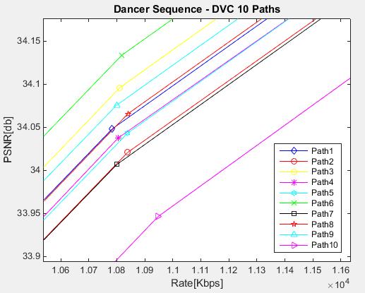
91 (a) (b) 91

92 (c) (d) Figure 4.7 Rate-Distortion Performance of DVC, for all 10 Paths; Zoom In for QP = 37 (a), QP = 32 (b), QP = 27 (c), QP = 22 (d) 92

93 DVC Decoding Strategies for WZFs (Interpolation Configurations) In order to obtain the comparison results, let us recall the Hybrid Scheme used in Free Navigation with DVC displayed in figure 3.2. Due to symmetry, the decoding strategies have been narrowed to four interpolation configuration. Let us denote them: Configuration 1: triplets as 111, 555, 999 highlighted in orange; Configuration 2: triplets as 155, 551, 955, 511, 995, 599, 115, 559 highlighted in blue; Configuration 3: triplets as 159, 951, 591, 915 highlighted in green; Configuration 4: triplets as 151, 959, 515, 595 highlighted in red; KF WZF KF WZF KF WZF KF WZF KF WZF KF Path Path Path Path Path Path Path Path Path Path Table 4.5 Decoding Strategies for WZFs (Interpolation Configurations) Configuration 1: Orange, Configuration 2: Blue, Configuration 3: Green, Configuration 4: Red During the experiments, 50 Wyner-Ziv frames (5 per each path) have been reconstructed during the DVC decoding; each PSNR and Rate attached to them were saved. In table 4.5 are synthesized and highlighted the decoding strategy used for each WZ frame, using a color-based ranking, as established before. 93

94 For the four decoding strategies (interpolation configurations), the average PSNR and Rate (per frame) have been computed for the four values of the Quantization Parameter. The results can be found in table 4.6. QP = 22 QP = 27 QP = 32 QP = 37 Average PSNR db Average Rate Kbps Average PSNR db Average Rate Kbps Average PSNR db Average Rate Kbps Average PSNR db Average Rate Kbps Configuration 1 Configuration 2 Configuration 3 Configuration Table 4.6 Average RD Performance Points (computed per Frame) for WZFs Interpolation Configurations with respect to QP Values It can be easily observed that Configurations 1 and 4 have the best Rate-Distortion values for the QP range, while Configurations 2 and 3 introduce a diminish in the quality of the frame (since PSNRs values are quite smaller and the Bit Rates increased). Figure 4.8 represents the RD curves or the four possible configurations; the similarity of Configurations 1 and 4 is present, on some portions the two curves overlap. Also, Configuration 3 is the one having the lowest performances. In table 4.7 can be found Rate-Distortion performance gain of the 4 configurations (decoding strategies) for WZFs, obtained with Bjontegaard metric. The letter R indicates which configurations has been used as the reference. Configuration 1 was compared to the other 3 configurations and the results are the following ones: it gives a PSNR improvement and a bandwidth saving with respect to all of them ( db and 0.123% - Configuration 4, db and % - Configuration 2, db and % - Configuration 3). The improvement in terms of both PNSR and Bit Rate with respect to Configuration 3 is huge, compared to the one with respect to Configuration 4. 94

95 Figure 4.8 Rate-Distortion Performance of DVC, for the Decoding Strategies (Interpolation Configurations) Since the improvement of Configuration 1 when the reference is Configuration 4 is almost inexistent, when comparing Configuration 4 to Configurations 2 and 3, a gain is similar to the one obtained for the first type: bandwidth saving of % and % and a PSNR gain of db and db. This makes clearer that the performances of Configuration 4 are better than performances of Configurations 2 and 3. Even though comparing Configurations 2 and 3 does not highlight a significant gain in terms of PSNR ( db for Configuration 2), the Bit Rate reduction is almost 6.5%. In conclusion, the Rate-Distortion performances for Configuration 1 are better than for the other 3 (although Configuration 4 can be an exception). In terms of the decoding strategy, it seems that reconstructing the Wyner-Ziv frame with side information obtained from 2 Key frames belonging to the same view as the original frame is the most accurate. Another interesting result is the one obtained for Configuration 4; it seems that reconstructing the Wyner-Ziv frame with side information obtained from 2 Key frames that belong to the same view (which is different to the view of the original frame) has the same accuracy as the above mentioned case. The worst case is the case when the I t,n WZF SI is obtained as the interpolation between I t 1,n 1 and I t+1,n+1 KFs, where n is the view number. The side information is not accurate, therefore 95