Chapter 4 FLUID KINEMATICS
|
|
|
- Coleen Reynolds
- 6 years ago
- Views:
Transcription
1 Fluid Mechanics: Fundamentals and Applications, 2nd Edition Yunus A. Cengel, John M. Cimbala McGraw-Hill, 2010 Chapter 4 FLUID KINEMATICS Lecture slides by Hasan Hacışevki Copyright The McGraw-Hill Companies, Inc. Permission required for reproduction or display.


2 Satellite image of a hurricane near the Florida coast; water droplets move with the air, enabling us to visualize the counterclockwise swirling motion. However, the major portion of the hurricane is actually irrotational, while only the core (the eye of the storm) is rotational. 2
3 Objectives Understand the role of the material derivative in transforming between Lagrangian and Eulerian descriptions Distinguish between various types of flow visualizations and methods of plotting the characteristics of a fluid flow Appreciate the many ways that fluids move and deform Distinguish between rotational and irrotational regions of flow based on the flow property vorticity Understand the usefulness of the Reynolds transport theorem 3

4 4 1 LAGRANGIAN AND EULERIAN DESCRIPTIONS Kinematics: The study of motion. Fluid kinematics: The study of how fluids flow and how to describe fluid motion. There are two distinct ways to describe motion: Lagrangian and Eulerian Lagrangian description: To follow the path of individual objects. This method requires us to track the position and velocity of each individual fluid parcel (fluid particle) and take to be a parcel of fixed identity. With a small number of objects, such as billiard balls on a pool table, individual objects can be tracked. In the Lagrangian description, one must keep track of the position and velocity of individual particles. 4
5 A more common method is Eulerian description of fluid motion. In the Eulerian description of fluid flow, a finite volume called a flow domain or control volume is defined, through which fluid flows in and out. Instead of tracking individual fluid particles, we define field variables, functions of space and time, within the control volume. The field variable at a particular location at a particular time is the value of the variable for whichever fluid particle happens to occupy that location at that time. For example, the pressure field is a scalar field variable. We define the velocity field as a vector field variable. Collectively, these (and other) field variables define the flow field. The velocity field can be expanded in Cartesian coordinates as 5

6 In the Eulerian description, one defines field variables, such as the pressure field and the velocity field, at any location and instant in time. In the Eulerian description we don t really care what happens to individual fluid particles; rather we are concerned with the pressure, velocity, acceleration, etc., of whichever fluid particle happens to be at the location of interest at the time of interest. While there are many occasions in which the Lagrangian description is useful, the Eulerian description is often more convenient for fluid mechanics applications. Experimental measurements are generally more suited to the Eulerian description. 6
7 7


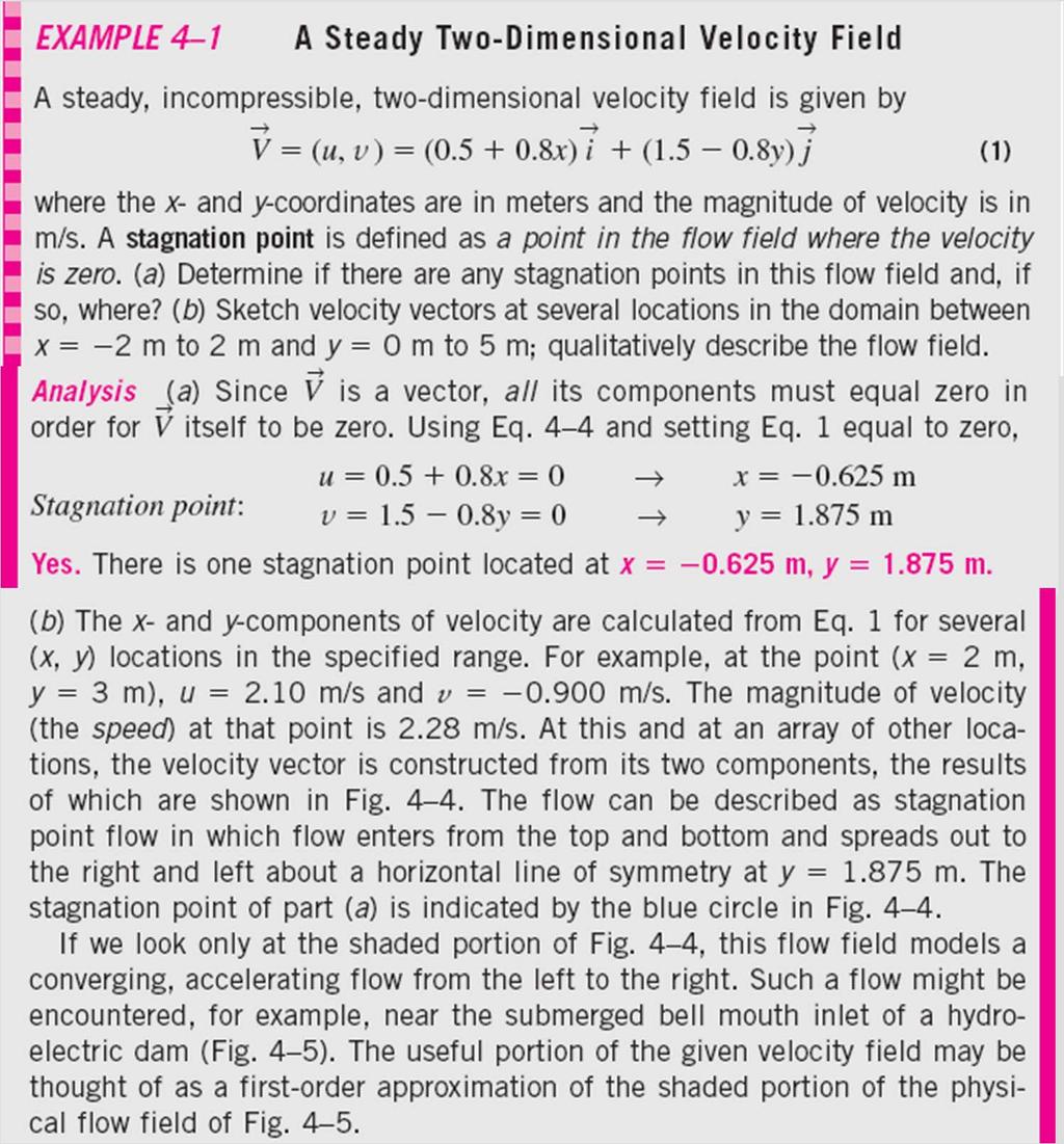
8 A Steady Two-Dimensional Velocity Field Flow field near the bell mouth inlet of a hydroelectric dam; a portion of the velocity field of Example 4-1 may be used as a first-order approximation of this physical flow field. Velocity vectors for the velocity field of Example 4 1. The scale is shown by the top arrow, and the solid black curves represent the approximate shapes of some streamlines, based on the calculated velocity vectors. The stagnation point is indicated by the circle. The shaded region represents a portion of the flow field that can approximate flow into an inlet. 8
9 Acceleration Field The equations of motion for fluid flow (such as Newton s second law) are written for a fluid particle, which we also call a material particle. If we were to follow a particular fluid particle as it moves around in the flow, we would be employing the Lagrangian description, and the equations of motion would be directly applicable. For example, we would define the particle s location in space in terms of a material position vector (x particle (t), y particle (t), z particle (t)). Newton s second law applied to a fluid particle; the acceleration vector (gray arrow) is in the same direction as the force vector (black arrow), but the velocity vector (red arrow) may act in a different direction. 9
 acceleration 10")
10 Local acceleration Advective (convective) acceleration 10
11 The components of the acceleration vector in cartesian coordinates: When following a fluid particle, the x- component of velocity, u, is defined as dx particle /dt. Similarly, v=dy particle /dt and w=dz particle /dt. Movement is shown here only in two dimensions for simplicity. Flow of water through the nozzle of a garden hose illustrates that fluid particles may accelerate, even in a steady flow. In this example, the exit speed of the water is much higher than the water speed in the hose, implying that fluid particles have accelerated even though the flow is steady. 11
12 Material Derivative The total derivative operator d/dt in this equation is given a special name, the material derivative; it is assigned a special notation, D/Dt, in order to emphasize that it is formed by following a fluid particle as it moves through the flow field. Other names for the material derivative include total, particle, Lagrangian, Eulerian, and substantial derivative. The material derivative D/Dt is defined by following a fluid particle as it moves throughout the flow field. In this illustration, the fluid particle is accelerating to the right as it moves up and to the right. 12

13 The material derivative D/Dt is composed of a local or unsteady part and a convective or advective part. 13
14 14
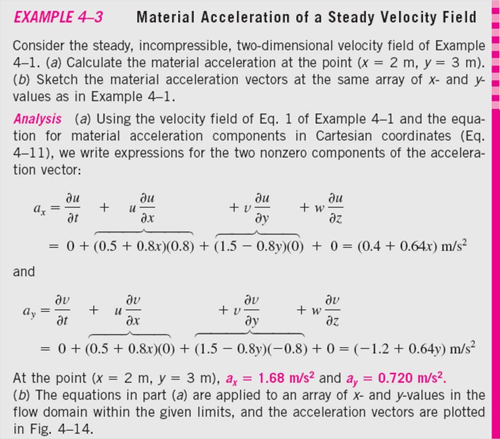
15 Material Acceleration of a Steady Velocity Field x Acceleration vectors for the velocity field of Examples 4 1 and 4 3. The scale is shown by the top arrow, and the solid black curves represent the approximate shapes of some streamlines, based on the calculated velocity vectors. The stagnation point is indicated by the color circle. 15

16 4 2 FLOW PATTERNS AND FLOW VISUALIZATION Flow visualization: The visual examination of flow field features. While quantitative study of fluid dynamics requires advanced mathematics, much can be learned from flow visualization. Flow visualization is useful not only in physical experiments but in numerical solutions as well [computational fluid dynamics (CFD)]. In fact, the very first thing an engineer using CFD does after obtaining a numerical solution is simulate some form of flow visualization. Spinning baseball. The late F. N. M. Brown devoted many years to developing and using smoke visualization in wind tunnels at the University of Notre Dame. Here the flow speed is about 23 m/s and the ball is rotated at 630 rpm. 16

17 Streamlines and Streamtubes Streamline: A curve that is everywhere tangent to the instantaneous local velocity vector. Streamlines are useful as indicators of the instantaneous direction of fluid motion throughout the flow field. For example, regions of recirculating flow and separation of a fluid off of a solid wall are easily identified by the streamline pattern. Streamlines cannot be directly observed experimentally except in steady flow fields. 17
18 18
19 19
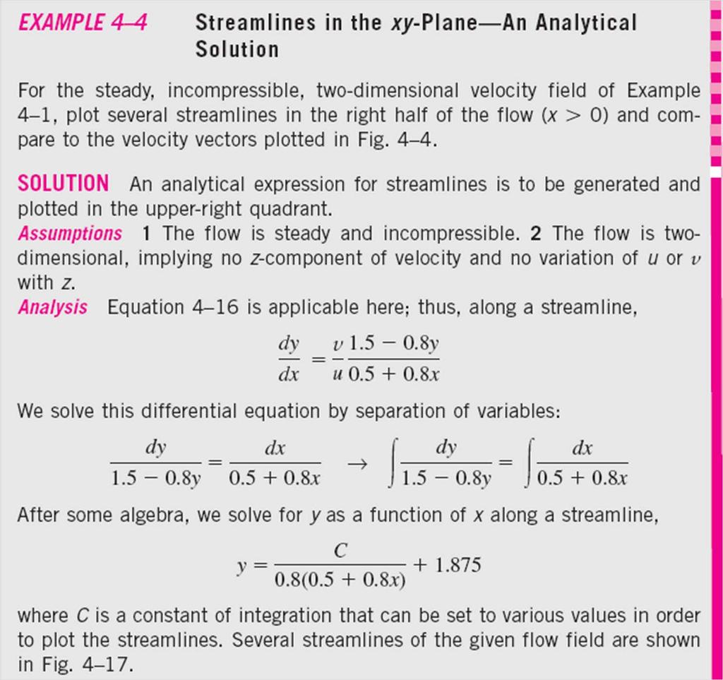
20 Streamlines for a steady, incompressible, two-dimensional velocity field Streamlines (solid black curves) for the velocity field of Example 4 4; velocity vectors (color arrows) are superimposed for comparison. The agreement is excellent in the sense that the velocity vectors point everywhere tangent to the streamlines. Note that speed cannot be determined directly from the streamlines alone. 20


21 A streamtube consists of a bundle of streamlines much like a communications cable consists of a bundle of fiber-optic cables. Since streamlines are everywhere parallel to the local velocity, fluid cannot cross a streamline by definition. Fluid within a streamtube must remain there and cannot cross the boundary of the streamtube. A streamtube consists of a bundle of individual streamlines. Both streamlines and streamtubes are instantaneous quantities, defined at a particular instant in time according to the velocity field at that instant. In an incompressible flow field, a streamtube (a) decreases in diameter as the flow accelerates or converges and (b) increases in diameter as the flow decelerates or diverges. 21

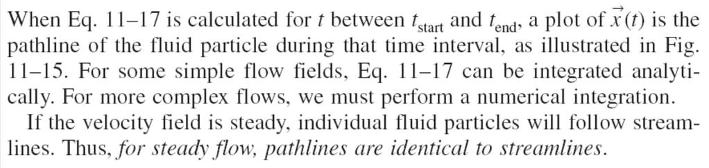
22 Pathlines Pathline: The actual path traveled by an individual fluid particle over some time period. A pathline is a Lagrangian concept in that we simply follow the path of an individual fluid particle as it moves around in the flow field. Thus, a pathline is the same as the fluid particle s material position vector (x particle (t), y particle (t), z particle (t)) traced out over some finite time interval. A pathline is formed by following the actual path of a fluid particle. Pathlines produced by white tracer particles suspended in water and captured by time-exposure photography; as waves pass horizontally, each particle moves in an elliptical path during one wave period. 22


23 Particle image velocimetry (PIV): A modern experimental technique that utilizes short segments of particle pathlines to measure the velocity field over an entire plane in a flow. Recent advances also extend the technique to three dimensions. In PIV, tiny tracer particles are suspended in the fluid. However, the flow is illuminated by two flashes of light (usually a light sheet from a laser) to produce two bright spots (recorded by a camera) for each moving particle. Then, both the magnitude and direction of the velocity vector at each particle location can be inferred, assuming that the tracer particles are small enough that they move with the fluid. Modern digital photography and fast computers have enabled PIV to be performed rapidly enough so that unsteady features of a flow field can also be measured. PIV applied to a model car in a wind tunnel. 23
24 24

25 Streaklines Streakline: The locus of fluid particles that have passed sequentially through a prescribed point in the flow. Streaklines are the most common flow pattern generated in a physical experiment. If you insert a small tube into a flow and introduce a continuous stream of tracer fluid (dye in a water flow or smoke in an air flow), the observed pattern is a streakline. A streakline is formed by continuous introduction of dye or smoke from a point in the flow. Labeled tracer particles (1 through 8) were introduced sequentially. 25

26 Streaklines produced by colored fluid introduced upstream; since the flow is steady, these streaklines are the same as streamlines and pathlines. Streaklines, streamlines, and pathlines are identical in steady flow but they can be quite different in unsteady flow. The main difference is that a streamline represents an instantaneous flow pattern at a given instant in time, while a streakline and a pathline are flow patterns that have some age and thus a time history associated with them. A streakline is an instantaneous snapshot of a time-integrated flow pattern. A pathline, on the other hand, is the time-exposed flow path of an individual particle over some time period. 26

27 In the figure, streaklines are introduced from a smoke wire located just downstream of a circular cylinder of diameter D aligned normal to the plane of view. When multiple streaklines are introduced along a line, as in the figure, we refer to this as a rake of streaklines. The Reynolds number of the flow is Re = 93. Smoke streaklines introduced by a smoke wire at two different locations in the wake of a circular cylinder: (a) smoke wire just downstream of the cylinder and (b) smoke wire located at x/d = 150. The time-integrative nature of streaklines 27 is clearly seen by comparing the two photographs.


28 Because of unsteady vortices shed in an alternating pattern from the cylinder, the smoke collects into a clearly defined periodic pattern called a Kármán vortex street. A similar pattern can be seen at much larger scale in the air flow in the wake of an island. Kármán vortices visible in the clouds in the wake of Alexander Selkirk Island in the southern Pacific Ocean. 28
29 29
30 Comparison of Flow Patterns in an Unsteady Flow An unsteady, incompressible, two-dimensional velocity field Streamlines, pathlines, and streaklines for the oscillating velocity field of Example 4 5. The streaklines and pathlines are wavy because of their integrated time history, but the streamlines are not wavy since they represent an instantaneous snapshot of the velocity field. 30
 is to be examined.")
31 Timelines Timeline: A set of adjacent fluid particles that were marked at the same (earlier) instant in time. Timelines are particularly useful in situations where the uniformity of a flow (or lack thereof) is to be examined. Timelines are formed by marking a line of fluid particles, and then watching that line move (and deform) through the flow field; timelines are shown at t = 0, t 1, t 2, and t 3. Timelines produced by a hydrogen bubble wire are used to visualize the boundary layer velocity profile shape. Flow is from left to right, and the hydrogen bubble wire is located to the left of the field of view. Bubbles near the wall reveal a flow instability that leads to turbulence. 31
32 Refractive Flow Visualization Techniques It is based on the refractive property of light waves. The speed of light through one material may differ somewhat from that in another material, or even in the same material if its density changes. As light travels through one fluid into a fluid with a different index of refraction, the light rays bend (they are refracted). Two primary flow visualization techniques that utilize the fact that the index of refraction in air (or other gases) varies with density: the shadowgraph technique and the schlieren technique. Interferometry is a visualization technique that utilizes the related phase change of light as it passes through air of varying densities as the basis for flow visualization. These techniques are useful for flow visualization in flow fields where density changes from one location in the flow to another, such as such as natural convection flows (temperature differences cause the density variations), mixing flows (fluid species cause the density variations), and supersonic flows (shock waves and expansion waves cause the density variations). 32

33 Unlike flow visualizations involving streaklines, pathlines, and timelines, the shadowgraph and schlieren methods do not require injection of a visible tracer (smoke or dye). Rather, density differences and the refractive property of light provide the necessary means for visualizing regions of activity in the flow field, allowing us to see the invisible. The image (a shadowgram) produced by the shadowgraph method is formed when the refracted rays of light rearrange the shadow cast onto a viewing screen or camera focal plane, causing bright or dark patterns to appear in the shadow. The dark patterns indicate the location where the refracted rays originate, while the bright patterns mark where these rays end up, and can be misleading. As a result, the dark regions are less distorted than the bright regions and are more useful in the interpretation of the shadowgram. Shadowgram of a 14.3 mm sphere in free flight through air at Ma 3.0. A shock wave is clearly visible in the shadow as a dark band that curves around the sphere and is called a bow wave (see Chap. 12). 33
 and a knife edge or other cutoff device to block the refracted light and is a true focused optical image.")
34 A shadowgram is not a true optical image; it is, after all, merely a shadow. A schlieren image, involves lenses (or mirrors) and a knife edge or other cutoff device to block the refracted light and is a true focused optical image. Schlieren imaging is more complicated to set up than is shadowgraphy but has a number of advantages. A schlieren image does not suffer from optical distortion by the refracted light rays. Schlieren imaging is also more sensitive to weak density gradients such as those caused by natural convection or by gradual phenomena like expansion fans in supersonic flow. Color schlieren imaging techniques have also been developed. One can adjust more components in a schlieren setup. Schlieren image of natural convection due to a barbeque grill. 34
35 Surface Flow Visualization Techniques The direction of fluid flow immediately above a solid surface can be visualized with tufts short, flexible strings glued to the surface at one end that point in the flow direction. Tufts are especially useful for locating regions of flow separation, where the flow direction suddenly reverses. A technique called surface oil visualization can be used for the same purpose oil placed on the surface forms streaks called friction lines that indicate the direction of flow. If it rains lightly when your car is dirty (especially in the winter when salt is on the roads), you may have noticed streaks along the hood and sides of the car, or even on the windshield. This is similar to what is observed with surface oil visualization. Lastly, there are pressure-sensitive and temperature-sensitive paints that enable researchers to observe the pressure or temperature distribution along solid surfaces. 35
36 4 3 PLOTS OF FLUID FLOW DATA Regardless of how the results are obtained (analytically, experimentally, or computationally), it is usually necessary to plot flow data in ways that enable the reader to get a feel for how the flow properties vary in time and/or space. You are already familiar with time plots, which are especially useful in turbulent flows (e.g., a velocity component plotted as a function of time), and xy-plots (e.g., pressure as a function of radius). In this section, we discuss three additional types of plots that are useful in fluid mechanics profile plots, vector plots, and contour plots. 36


37 Profile Plots A profile plot indicates how the value of a scalar property varies along some desired direction in the flow field. In fluid mechanics, profile plots of any scalar variable (pressure, temperature, density, etc.) can be created, but the most common one used in this book is the velocity profile plot. Since velocity is a vector quantity, we usually plot either the magnitude of velocity or one of the components of the velocity vector as a function of distance in some desired direction. Profile plots of the horizontal component of velocity as a function of vertical distance; flow in the boundary layer growing along a horizontal flat plate: (a) standard profile plot and (b) profile plot with arrows. 37
.")
38 Vector Plots A vector plot is an array of arrows indicating the magnitude and direction of a vector property at an instant in time. Streamlines indicate the direction of the instantaneous velocity field, they do not directly indicate the magnitude of the velocity (i.e., the speed). A useful flow pattern for both experimental and computational fluid flows is thus the vector plot, which consists of an array of arrows that indicate both magnitude and direction of an instantaneous vector property. Vector plots can also be generated from experimentally obtained data (e.g., from PIV measurements) or numerically from CFD calculations. Fig. 4-4: Velocity vector plot Fig. 4-14: Acceleration vector plot. Both generated analytically. 38

 velocity vector plot, close-up view revealing more details in the")
39 Results of CFD calculations of a twodimensional flow field consisting of free-stream flow impinging on a block of rectangular cross section. (a) streamlines, (b) velocity vector plot of the upper half of the flow, and (c) velocity vector plot, close-up view revealing more details in the separated flow region. 39
 are generated of pressure, temperature, velocity magnitude, species concentration, properties of turbulence, etc.")
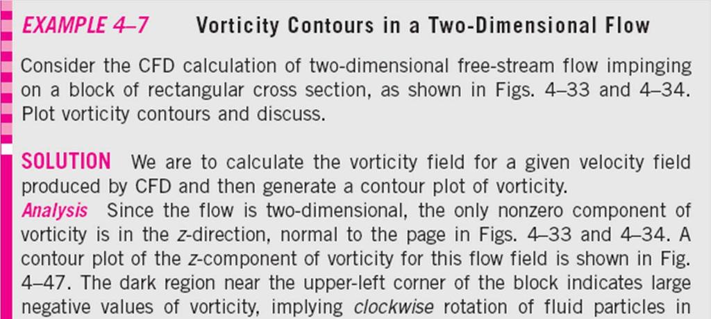
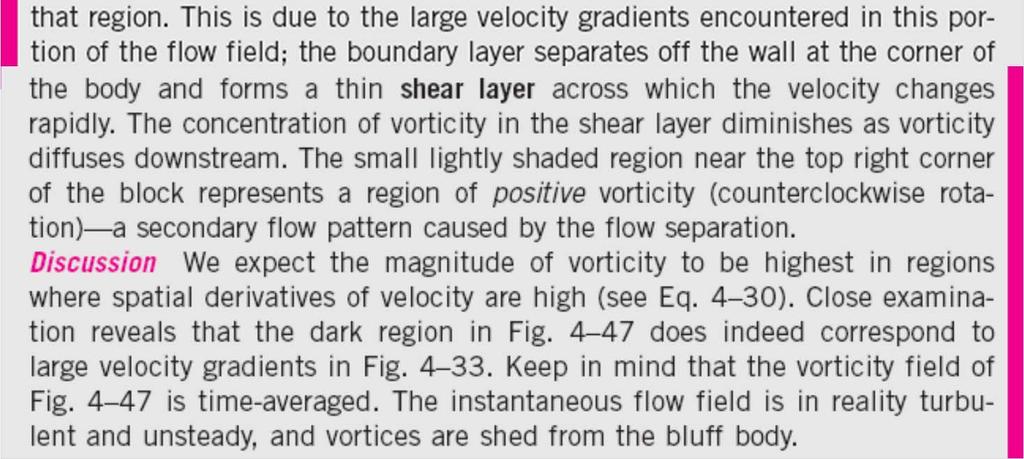
40 A contour plot shows curves of constant values of a scalar property (or magnitude of a vector property) at an instant in time. Contour Plots Contour plots (also called isocontour plots) are generated of pressure, temperature, velocity magnitude, species concentration, properties of turbulence, etc. A contour plot can quickly reveal regions of high (or low) values of the flow property being studied. A contour plot may consist simply of curves indicating various levels of the property; this is called a contour line plot. Alternatively, the contours can be filled in with either colors or shades of gray; this is called a filled contour plot. Contour plots of the pressure field due to flow impinging on a block, as produced by CFD calculations; only the upper half is shown due to symmetry; (a) filled gray scale contour plot and (b) contour line plot where pressure values are displayed in units of Pa gage pressure. 40
 linear strain (also called extensional strain), and (d) shear strain. All four types of motion or deformation usually occur simultaneously.")
41 4 4 OTHER KINEMATIC DESCRIPTIONS Types of Motion or Deformation of Fluid Elements In fluid mechanics, an element may undergo four fundamental types of motion or deformation: (a) translation, (b) rotation, (c) linear strain (also called extensional strain), and (d) shear strain. All four types of motion or deformation usually occur simultaneously. It is preferable in fluid dynamics to describe the motion and deformation of fluid elements in terms of rates such as velocity (rate of translation), angular velocity (rate of rotation), linear strain rate (rate of linear strain), and shear strain rate (rate of shear strain). In order for these deformation rates to be useful in the calculation of fluid flows, we must express them in terms of velocity and derivatives of velocity. Fundamental types of fluid element motion or deformation: (a) translation, (b) rotation, (c) linear strain, 41 and (d) shear strain.
 at a point: The average rotation rate of two initially perpendicular lines that intersect at that point.")
42 A vector is required in order to fully describe the rate of translation in three dimensions. The rate of translation vector is described mathematically as the velocity vector. Rate of rotation (angular velocity) at a point: The average rotation rate of two initially perpendicular lines that intersect at that point. Rate of rotation of fluid element about point P For a fluid element that translates and deforms as sketched, the rate of rotation at point P is defined as the average rotation rate of two initially perpendicular lines (lines a and b). 42
43 The rate of rotation vector is equal to the angular velocity vector. Linear strain rate: The rate of increase in length per unit length. Mathematically, the linear strain rate of a fluid element depends on the initial orientation or direction of the line segment upon which we measure the linear strain. 43

44 Using the lengths marked in the figure, the linear strain rate in the x a -direction is 44
 when exposed to dim light).")
45 Volumetric strain rate or bulk strain rate: The rate of increase of volume of a fluid element per unit volume. This kinematic property is defined as positive when the volume increases. Another synonym of volumetric strain rate is also called rate of volumetric dilatation, (the iris of your eye dilates (enlarges) when exposed to dim light). The volumetric strain rate is the sum of the linear strain rates in three mutually orthogonal directions. The volumetric strain rate is zero in an incompressible flow. Air being compressed by a piston in a cylinder; the volume of a fluid element in the cylinder decreases, corresponding to a negative rate of volumetric dilatation. 45
46 Shear strain rate at a point: Half of the rate of decrease of the angle between two initially perpendicular lines that intersect at the point. Shear strain rate, initially perpendicular lines in the x- and y-directions: Shear strain rate in Cartesian coordinates: For a fluid element that translates and deforms as sketched, the shear strain rate at point P is defined as half of the rate of decrease of the angle between two initially perpendicular lines (lines a and b). 46
47 Figure shows a general (although two-dimensional) situation in a compressible fluid flow in which all possible motions and deformations are present simultaneously. In particular, there is translation, rotation, linear strain, and shear strain. Because of the compressible nature of the fluid flow, there is also volumetric strain (dilatation). You should now have a better appreciation of the inherent complexity of fluid dynamics, and the mathematical sophistication required to fully describe fluid motion. A fluid element illustrating translation, rotation, linear strain, shear strain, and volumetric strain. 47
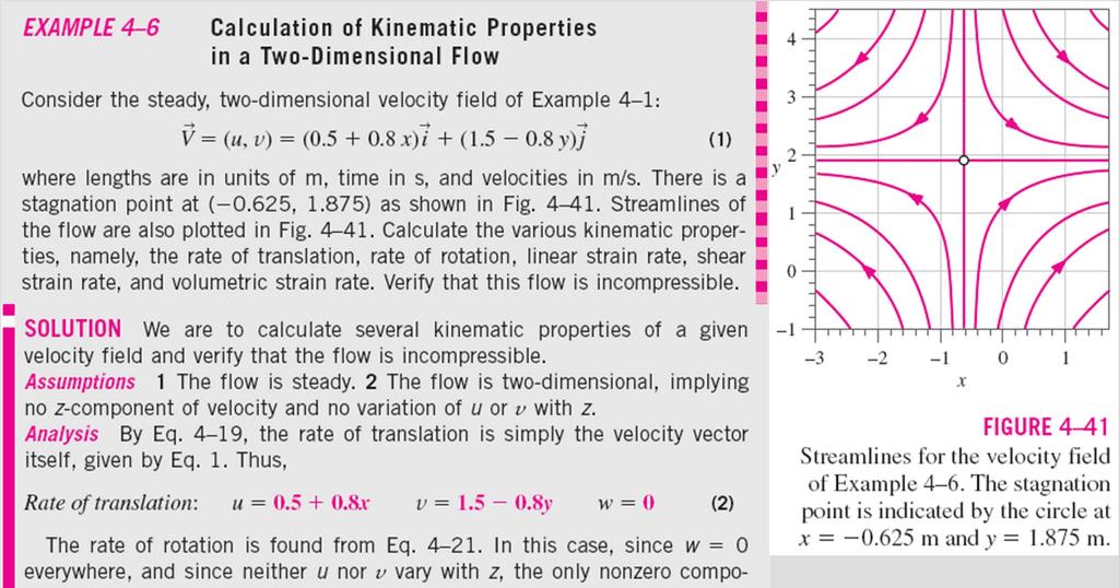
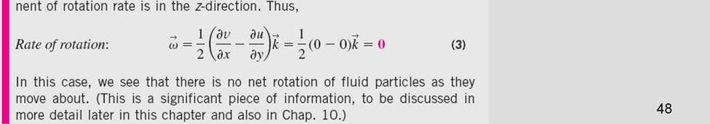
48 48
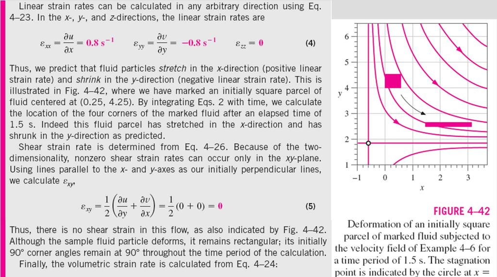
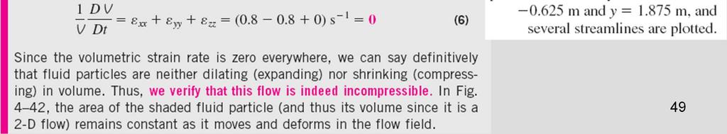
49 49

50 4 5 VORTICITY AND ROTATIONALITY Another kinematic property of great importance to the analysis of fluid flows is the vorticity vector, defined mathematically as the curl of the velocity vector Vorticity is equal to twice the angular velocity of a fluid particle The direction of a vector cross product is determined by the righthand rule. The vorticity vector is equal to twice the angular velocity vector of a rotating fluid particle. 50
, fluid particles there are not rotating; the flow in that region is called irrotational.")
51 If the vorticity at a point in a flow field is nonzero, the fluid particle that happens to occupy that point in space is rotating; the flow in that region is called rotational. Likewise, if the vorticity in a region of the flow is zero (or negligibly small), fluid particles there are not rotating; the flow in that region is called irrotational. Physically, fluid particles in a rotational region of flow rotate end over end as they move along in the flow. The difference between rotational and irrotational flow: fluid elements in a rotational region of the flow rotate, but those in an irrotational region of the flow do not. 51

52 For a two-dimensional flow in the xy-plane, the vorticity vector always points in the z- or z-direction. In this illustration, the flag-shaped fluid particle rotates in the counterclockwise direction as it moves in the xy-plane; its vorticity points in the positive z-direction as shown. 52
53 53
54 54

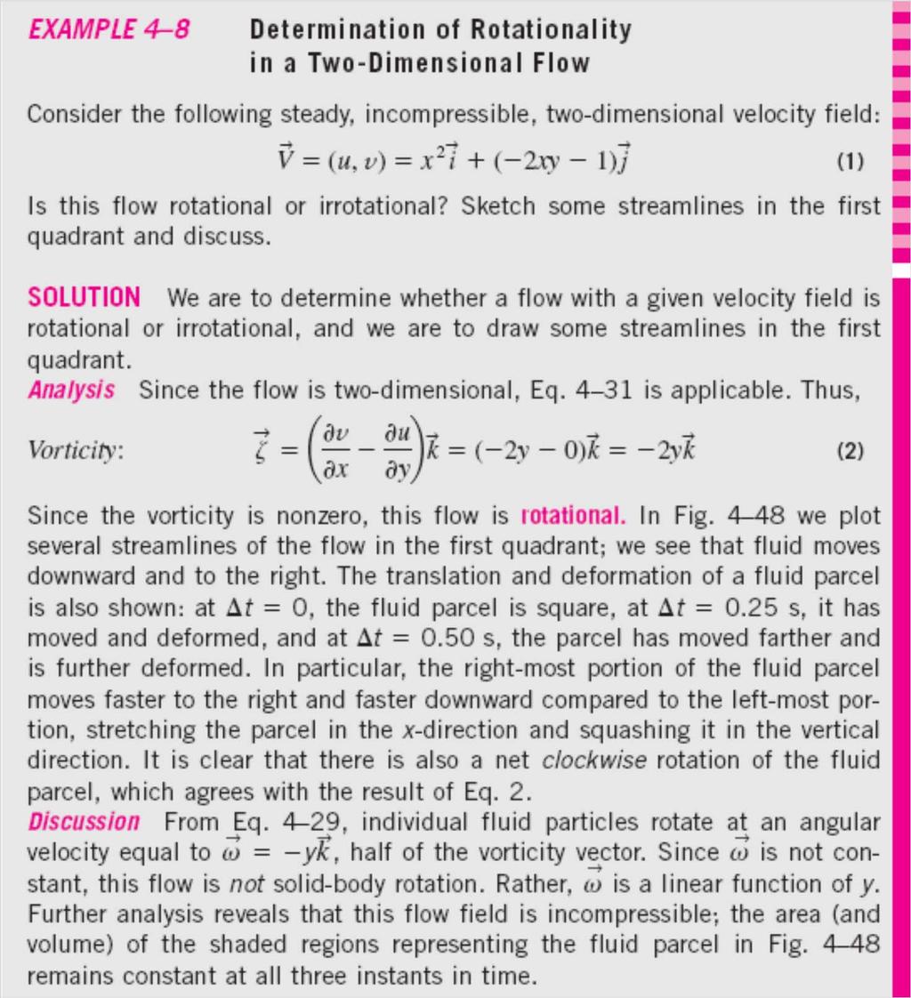
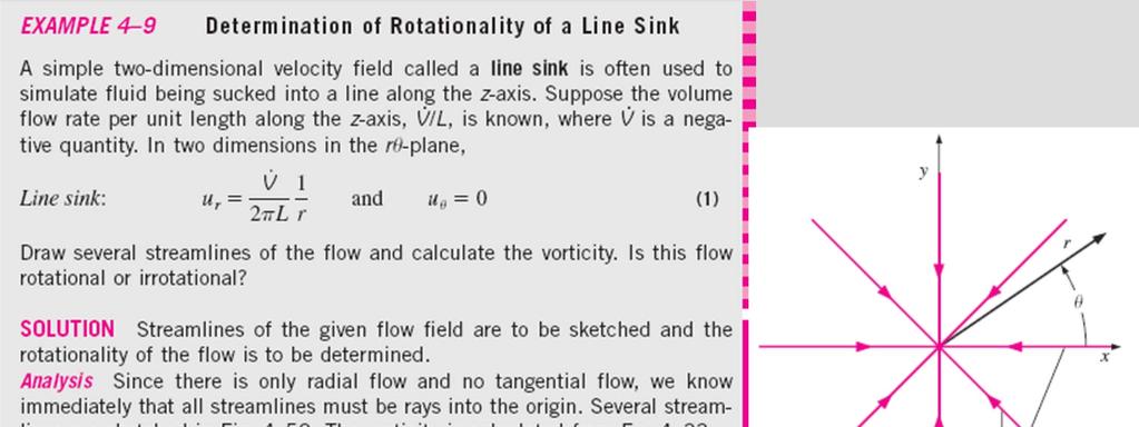
55 Determination of Rotationality in a Two-Dimensional Flow steady, incompressible, twodimensional velocity field: Vorticity: Deformation of an initially square fluid parcel subjected to the velocity field of Example 4 8 for a time period of 0.25 s and 0.50 s. Several streamlines are also plotted in the first quadrant. It is clear that this flow is rotational. 55

56 For a two-dimensional flow in the r plane, the vorticity vector always points in the z (or z) direction. In this illustration, the flag-shaped fluid particle rotates in the clockwise direction as it moves in the ru-plane; its vorticity points in the z-direction as shown. 56
57 Comparison of Two Circular Flows Streamlines and velocity profiles for (a) flow A, solid-body rotation and (b) flow B, a line vortex. Flow A is rotational, but flow B is irrotational everywhere except at the origin. 57


58 A simple analogy can be made between flow A and a merry-goround or roundabout, and flow B and a Ferris wheel. As children revolve around a roundabout, they also rotate at the same angular velocity as that of the ride itself. This is analogous to a rotational flow. In contrast, children on a Ferris wheel always remain oriented in an upright position as they trace out their circular path. This is analogous to an irrotational flow. A simple analogy: (a) rotational circular flow is analogous to a roundabout, while (b) irrotational circular flow is analogous to a Ferris wheel. 58
59 59
 We consider a fixed interior volume of the can.")
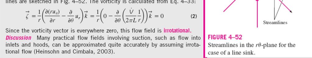
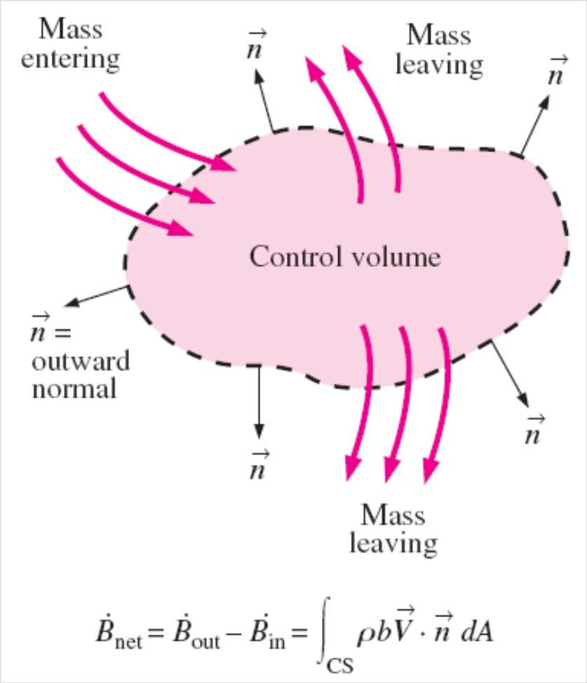
60 4 6 THE REYNOLDS TRANSPORT THEOREM Two methods of analyzing the spraying of deodorant from a spray can: (a) We follow the fluid as it moves and deforms. This is the system approach no mass crosses the boundary, and the total mass of the system remains fixed. (b) We consider a fixed interior volume of the can. This is the control volume approach mass crosses the boundary. The relationship between the time rates of change of an extensive property for a system and for a control volume is expressed by the Reynolds transport theorem (RTT). The Reynolds transport theorem (RTT) provides a link between the system approach and the control volume approach. 60

61 The time rate of change of the property B of the system is equal to the time rate of change of B of the control volume plus the net flux of B out of the control volume by mass crossing the control surface. This equation applies at any instant in time, where it is assumed that the system and the control volume occupy the same space at that particular instant in time. A moving system (hatched region) and a fixed control volume (shaded region) in a diverging portion of a flow field at times t and t+ t. The upper and lower bounds are streamlines of the flow. 61
62 62
63 63

64 Reynolds transport theorem applied to a control volume moving at constant velocity. Relative velocity crossing a control surface is found by vector addition of the absolute velocity of the fluid and the negative of the local velocity of the control surface. 64

65 An example control volume in which there is one well-defined inlet (1) and two well-defined outlets (2 and 3). In such cases, the control surface integral in the RTT can be more conveniently written in terms of the average values of fluid properties crossing each inlet and outlet. 65
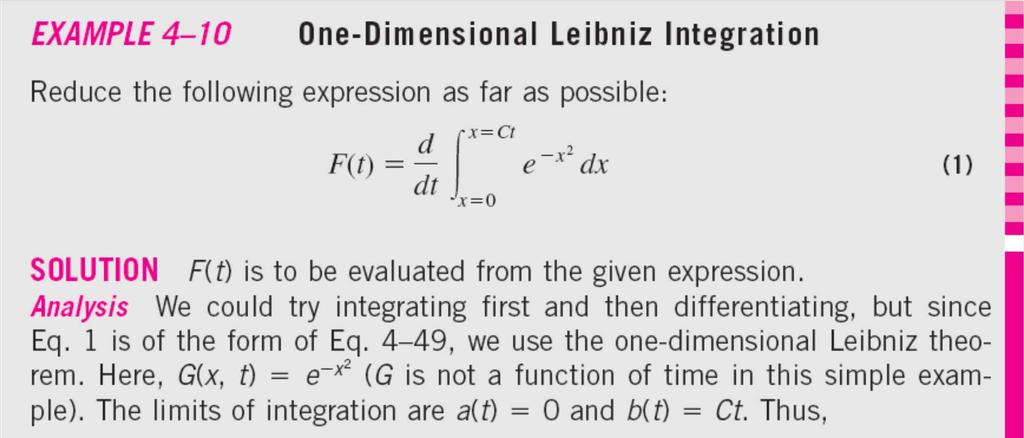
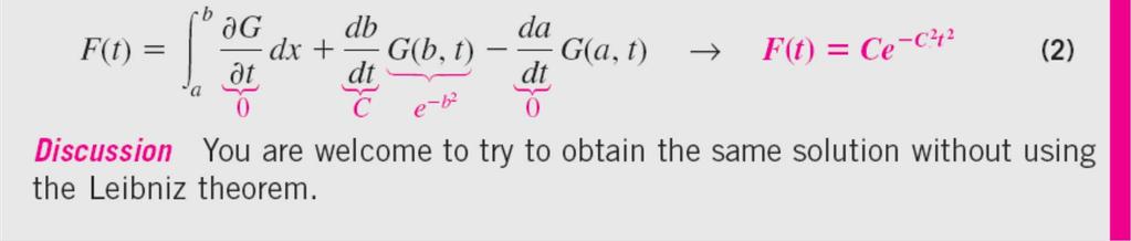
 and b(t) with respect to time, as well as the unsteady changes of integrand G(x, t) with time.")
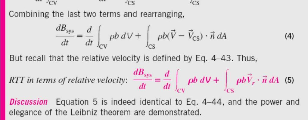
66 Alternate Derivation of the Reynolds Transport Theorem A more elegant mathematical derivation of the Reynolds transport theorem is possible through use of the Leibniz theorem The Leibniz theorem takes into account the change of limits a(t) and b(t) with respect to time, as well as the unsteady changes of integrand G(x, t) with time. 66
67 67
68 68

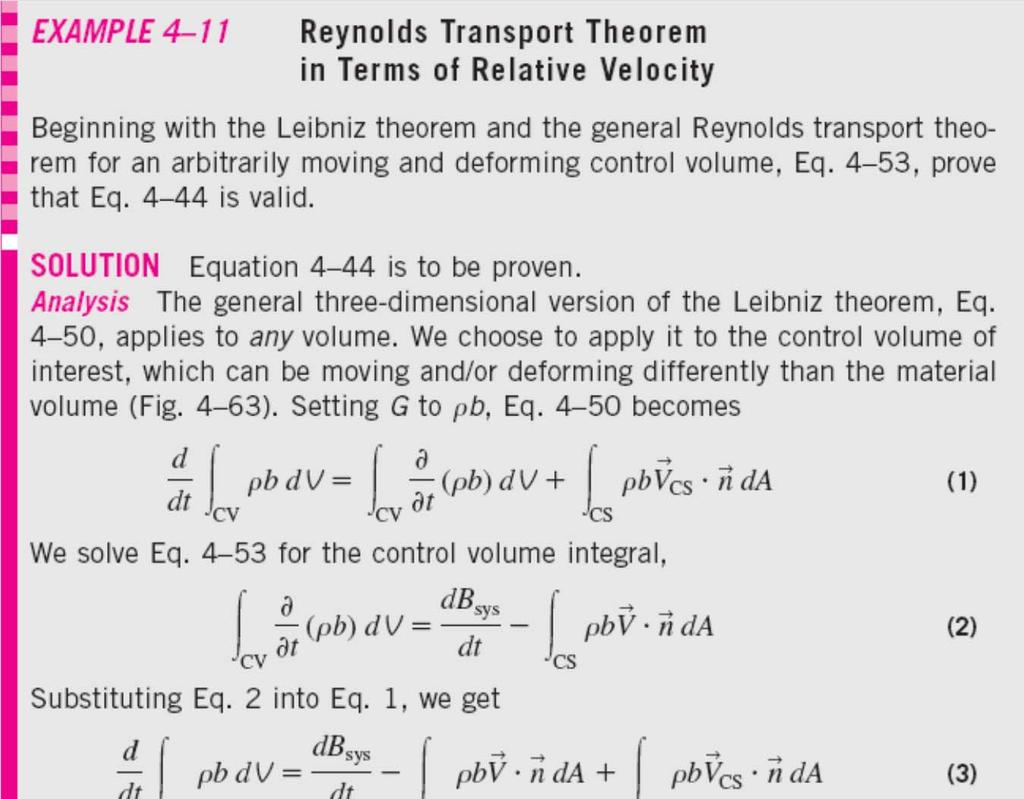
69 The three-dimensional Leibniz theorem is required when calculating the time derivative of a volume integral for which the volume itself moves and/or deforms with time. It turns out that the three-dimensional form of the Leibniz theorem can be used in an alternative derivation of the Reynolds transport theorem. 69
, but move and deform differently. At a later time they are not coincident.")
70 The material volume (system) and control volume occupy the same space at time t (the blue shaded area), but move and deform differently. At a later time they are not coincident. 70
71 71
. In both cases, we transform from a Lagrangian or system viewpoint to an Eulerian or control volume viewpoint.")
72 Relationship between Material Derivative and RTT The Reynolds transport theorem for finite volumes (integral analysis) is analogous to the material derivative for infinitesimal volumes (differential analysis). In both cases, we transform from a Lagrangian or system viewpoint to an Eulerian or control volume viewpoint. While the Reynolds transport theorem deals with finite-size control volumes and the material derivative deals with infinitesimal fluid particles, the same fundamental physical interpretation applies to both. Just as the material derivative can be applied to any fluid property, scalar or vector, the Reynolds transport theorem can be applied to any scalar or vector property as well. 72
73 Summary Lagrangian and Eulerian Descriptions Acceleration Field Material Derivative Flow Patterns and Flow Visualization Streamlines and Streamtubes, Pathlines, Streaklines, Timelines Refractive Flow Visualization Techniques Surface Flow Visualization Techniques Plots of Fluid Flow Data Vector Plots, Contour Plots Other Kinematic Descriptions Types of Motion or Deformation of Fluid Elements Vorticity and Rotationality Comparison of Two Circular Flows The Reynolds Transport Theorem Alternate Derivation of the Reynolds Transport Theorem Relationship between Material Derivative and RTT 73
MAE 3130: Fluid Mechanics Lecture 5: Fluid Kinematics Spring Dr. Jason Roney Mechanical and Aerospace Engineering
 MAE 3130: Fluid Mechanics Lecture 5: Fluid Kinematics Spring 2003 Dr. Jason Roney Mechanical and Aerospace Engineering Outline Introduction Velocity Field Acceleration Field Control Volume and System Representation
FLOWING FLUIDS AND PRESSURE VARIATION
 Chapter 4 Pressure differences are (often) the forces that move fluids FLOWING FLUIDS AND PRESSURE VARIATION Fluid Mechanics, Spring Term 2011 e.g., pressure is low at the center of a hurricane. For your
Vector Visualization. CSC 7443: Scientific Information Visualization
 Vector Visualization Vector data A vector is an object with direction and length v = (v x,v y,v z ) A vector field is a field which associates a vector with each point in space The vector data is 3D representation
Lecture 1.1 Introduction to Fluid Dynamics
 Lecture 1.1 Introduction to Fluid Dynamics 1 Introduction A thorough study of the laws of fluid mechanics is necessary to understand the fluid motion within the turbomachinery components. In this introductory
Chapter 5: Introduction to Differential Analysis of Fluid Motion
 Chapter 5: Introduction to Differential 5-1 Conservation of Mass 5-2 Stream Function for Two-Dimensional 5-3 Incompressible Flow 5-4 Motion of a Fluid Particle (Kinematics) 5-5 Momentum Equation 5-6 Computational
Lagrangian and Eulerian Representations of Fluid Flow: Kinematics and the Equations of Motion
 Lagrangian and Eulerian Representations of Fluid Flow: Kinematics and the Equations of Motion James F. Price Woods Hole Oceanographic Institution Woods Hole, MA, 02543 July 31, 2006 Summary: This essay
Measurements in Fluid Mechanics
 Measurements in Fluid Mechanics 13.1 Introduction The purpose of this chapter is to provide the reader with a basic introduction to the concepts and techniques applied by engineers who measure flow parameters
1 Mathematical Concepts
 1 Mathematical Concepts Mathematics is the language of geophysical fluid dynamics. Thus, in order to interpret and communicate the motions of the atmosphere and oceans. While a thorough discussion of the
Using Flow Visualization for PCB Thermal Design and Optimization
 Thermal Minutes Using Flow Visualization for PCB Thermal Design and Optimization FLOW DIRECTION Figure 1. Top View of Flow Around Equal Sized Components, Depicting Reversed Flow in the Wake of the Component
FLUID MECHANICS TESTS
 FLUID MECHANICS TESTS Attention: there might be more correct answers to the questions. Chapter 1: Kinematics and the continuity equation T.2.1.1A flow is steady if a, the velocity direction of a fluid
Chapter 1 - Basic Equations
 2.20 Marine Hydrodynamics, Fall 2017 Lecture 2 Copyright c 2017 MIT - Department of Mechanical Engineering, All rights reserved. 2.20 Marine Hydrodynamics Lecture 2 Chapter 1 - Basic Equations 1.1 Description
The viscous forces on the cylinder are proportional to the gradient of the velocity field at the
 Fluid Dynamics Models : Flow Past a Cylinder Flow Past a Cylinder Introduction The flow of fluid behind a blunt body such as an automobile is difficult to compute due to the unsteady flows. The wake behind
Inviscid Flows. Introduction. T. J. Craft George Begg Building, C41. The Euler Equations. 3rd Year Fluid Mechanics
 Contents: Navier-Stokes equations Inviscid flows Boundary layers Transition, Reynolds averaging Mixing-length models of turbulence Turbulent kinetic energy equation One- and Two-equation models Flow management
Flow Structures Extracted from Visualization Images: Vector Fields and Topology
 Flow Structures Extracted from Visualization Images: Vector Fields and Topology Tianshu Liu Department of Mechanical & Aerospace Engineering Western Michigan University, Kalamazoo, MI 49008, USA We live
FLUENT Secondary flow in a teacup Author: John M. Cimbala, Penn State University Latest revision: 26 January 2016
 FLUENT Secondary flow in a teacup Author: John M. Cimbala, Penn State University Latest revision: 26 January 2016 Note: These instructions are based on an older version of FLUENT, and some of the instructions
Driven Cavity Example
 BMAppendixI.qxd 11/14/12 6:55 PM Page I-1 I CFD Driven Cavity Example I.1 Problem One of the classic benchmarks in CFD is the driven cavity problem. Consider steady, incompressible, viscous flow in a square
Prerequisites: This tutorial assumes that you are familiar with the menu structure in FLUENT, and that you have solved Tutorial 1.
 Tutorial 22. Postprocessing Introduction: In this tutorial, the postprocessing capabilities of FLUENT are demonstrated for a 3D laminar flow involving conjugate heat transfer. The flow is over a rectangular
Laser speckle based background oriented schlieren measurements in a fire backlayering front
 Laser speckle based background oriented schlieren measurements in a fire backlayering front Philipp Bühlmann 1*, Alexander H. Meier 1, Martin Ehrensperger 1, Thomas Rösgen 1 1: ETH Zürich, Institute of
SPC 307 Aerodynamics. Lecture 1. February 10, 2018
 SPC 307 Aerodynamics Lecture 1 February 10, 2018 Sep. 18, 2016 1 Course Materials drahmednagib.com 2 COURSE OUTLINE Introduction to Aerodynamics Review on the Fundamentals of Fluid Mechanics Euler and
SolidWorks Flow Simulation 2014
 An Introduction to SolidWorks Flow Simulation 2014 John E. Matsson, Ph.D. SDC PUBLICATIONS Better Textbooks. Lower Prices. www.sdcpublications.com Powered by TCPDF (www.tcpdf.org) Visit the following websites
An Introduction to SolidWorks Flow Simulation 2010
 An Introduction to SolidWorks Flow Simulation 2010 John E. Matsson, Ph.D. SDC PUBLICATIONS www.sdcpublications.com Schroff Development Corporation Chapter 2 Flat Plate Boundary Layer Objectives Creating
Pulsating flow around a stationary cylinder: An experimental study
 Proceedings of the 3rd IASME/WSEAS Int. Conf. on FLUID DYNAMICS & AERODYNAMICS, Corfu, Greece, August 2-22, 2 (pp24-244) Pulsating flow around a stationary cylinder: An experimental study A. DOUNI & D.
Estimating Vertical Drag on Helicopter Fuselage during Hovering
 Estimating Vertical Drag on Helicopter Fuselage during Hovering A. A. Wahab * and M.Hafiz Ismail ** Aeronautical & Automotive Dept., Faculty of Mechanical Engineering, Universiti Teknologi Malaysia, 81310
CFD MODELING FOR PNEUMATIC CONVEYING
 CFD MODELING FOR PNEUMATIC CONVEYING Arvind Kumar 1, D.R. Kaushal 2, Navneet Kumar 3 1 Associate Professor YMCAUST, Faridabad 2 Associate Professor, IIT, Delhi 3 Research Scholar IIT, Delhi e-mail: arvindeem@yahoo.co.in
Essay 1: Dimensional Analysis of Models and Data Sets: Similarity Solutions
 Table of Contents Essay 1: Dimensional Analysis of Models and Data Sets: Similarity Solutions and Scaling Analysis 1 About dimensional analysis 4 1.1 Thegoalandtheplan... 4 1.2 Aboutthisessay... 5 2 Models
Lecture # 16: Review for Final Exam
 AerE 344 Lecture Notes Lecture # 6: Review for Final Exam Hui Hu Department of Aerospace Engineering, Iowa State University Ames, Iowa 5, U.S.A AerE343L: Dimensional Analysis and Similitude Commonly used
Simulation of Flow Development in a Pipe
 Tutorial 4. Simulation of Flow Development in a Pipe Introduction The purpose of this tutorial is to illustrate the setup and solution of a 3D turbulent fluid flow in a pipe. The pipe networks are common
Preliminary Spray Cooling Simulations Using a Full-Cone Water Spray
 39th Dayton-Cincinnati Aerospace Sciences Symposium Preliminary Spray Cooling Simulations Using a Full-Cone Water Spray Murat Dinc Prof. Donald D. Gray (advisor), Prof. John M. Kuhlman, Nicholas L. Hillen,
Rotating Moving Boundary Analysis Using ANSYS 5.7
 Abstract Rotating Moving Boundary Analysis Using ANSYS 5.7 Qin Yin Fan CYBERNET SYSTEMS CO., LTD. Rich Lange ANSYS Inc. As subroutines in commercial software, APDL (ANSYS Parametric Design Language) provides
Flow Field of Truncated Spherical Turrets
 Flow Field of Truncated Spherical Turrets Kevin M. Albarado 1 and Amelia Williams 2 Aerospace Engineering, Auburn University, Auburn, AL, 36849 Truncated spherical turrets are used to house cameras and
Introduction to C omputational F luid Dynamics. D. Murrin
 Introduction to C omputational F luid Dynamics D. Murrin Computational fluid dynamics (CFD) is the science of predicting fluid flow, heat transfer, mass transfer, chemical reactions, and related phenomena
COMPUTATIONAL AND EXPERIMENTAL INTERFEROMETRIC ANALYSIS OF A CONE-CYLINDER-FLARE BODY. Abstract. I. Introduction
 COMPUTATIONAL AND EXPERIMENTAL INTERFEROMETRIC ANALYSIS OF A CONE-CYLINDER-FLARE BODY John R. Cipolla 709 West Homeway Loop, Citrus Springs FL 34434 Abstract A series of computational fluid dynamic (CFD)
Automated calculation report (example) Date 05/01/2018 Simulation type
 Date 05/01/2018 Simulation type") Automated calculation report (example) Project name Tesla Semi Date 05/01/2018 Simulation type Moving Table of content Contents Table of content... 2 Introduction... 3 Project details... 3 Disclaimer...
Automated calculation report (example) Project name Tesla Semi Date 05/01/2018 Simulation type Moving Table of content Contents Table of content... 2 Introduction... 3 Project details... 3 Disclaimer...
Example 13 - Shock Tube
 Example 13 - Shock Tube Summary This famous experiment is interesting for observing the shock-wave propagation. Moreover, this case uses the representation of perfect gas and compares the different formulations:
Particle Velocimetry Data from COMSOL Model of Micro-channels
 Particle Velocimetry Data from COMSOL Model of Micro-channels P.Mahanti *,1, M.Keebaugh 1, N.Weiss 1, P.Jones 1, M.Hayes 1, T.Taylor 1 Arizona State University, Tempe, Arizona *Corresponding author: GWC
CFD Analysis of a Fully Developed Turbulent Flow in a Pipe with a Constriction and an Obstacle
 CFD Analysis of a Fully Developed Turbulent Flow in a Pipe with a Constriction and an Obstacle C, Diyoke Mechanical Engineering Department Enugu State University of Science & Tech. Enugu, Nigeria U, Ngwaka
Modeling & Simulation of Supersonic Flow Using McCormack s Technique
 Modeling & Simulation of Supersonic Flow Using McCormack s Technique M. Saif Ullah Khalid*, Afzaal M. Malik** Abstract In this work, two-dimensional inviscid supersonic flow around a wedge has been investigated
Vector Visualization
 Vector Visualization Vector Visulization Divergence and Vorticity Vector Glyphs Vector Color Coding Displacement Plots Stream Objects Texture-Based Vector Visualization Simplified Representation of Vector
GLASGOW 2003 INTEGRATING CFD AND EXPERIMENT
 GLASGOW 2003 INTEGRATING CFD AND EXPERIMENT A Detailed CFD and Experimental Investigation of a Benchmark Turbulent Backward Facing Step Flow Stephen Hall & Tracie Barber University of New South Wales Sydney,
CFD Analysis of 2-D Unsteady Flow Past a Square Cylinder at an Angle of Incidence
 CFD Analysis of 2-D Unsteady Flow Past a Square Cylinder at an Angle of Incidence Kavya H.P, Banjara Kotresha 2, Kishan Naik 3 Dept. of Studies in Mechanical Engineering, University BDT College of Engineering,
Lecture # 11: Particle image velocimetry
 AerE 344 Lecture Notes Lecture # 11: Particle image velocimetry Dr. Hui Hu Dr. Rye M Waldman Department of Aerospace Engineering Iowa State University Ames, Iowa 50011, U.S.A Sources/ Further reading:
Compressible Flow in a Nozzle
 SPC 407 Supersonic & Hypersonic Fluid Dynamics Ansys Fluent Tutorial 1 Compressible Flow in a Nozzle Ahmed M Nagib Elmekawy, PhD, P.E. Problem Specification Consider air flowing at high-speed through a
PHYS:1200 LECTURE 32 LIGHT AND OPTICS (4)
") 1 PHYS:1200 LECTURE 32 LIGHT AND OPTICS (4) The first three lectures in this unit dealt with what is for called geometric optics. Geometric optics, treats light as a collection of rays that travel in straight
1 PHYS:1200 LECTURE 32 LIGHT AND OPTICS (4) The first three lectures in this unit dealt with what is for called geometric optics. Geometric optics, treats light as a collection of rays that travel in straight
SYNTHETIC SCHLIEREN. Stuart B Dalziel, Graham O Hughes & Bruce R Sutherland. Keywords: schlieren, internal waves, image processing
 8TH INTERNATIONAL SYMPOSIUM ON FLOW VISUALIZATION (998) SYNTHETIC SCHLIEREN Keywords: schlieren, internal waves, image processing Abstract This paper outlines novel techniques for producing qualitative
Optics INTRODUCTION DISCUSSION OF PRINCIPLES. Reflection by a Plane Mirror
 Optics INTRODUCTION Geometric optics is one of the oldest branches of physics, dealing with the laws of reflection and refraction. Reflection takes place on the surface of an object, and refraction occurs
Data Visualization. Fall 2017
 Data Visualization Fall 2017 Vector Fields Vector field v: D R n D is typically 2D planar surface or 2D surface embedded in 3D n = 2 fields tangent to 2D surface n = 3 volumetric fields When visualizing
Modeling Evaporating Liquid Spray
 Tutorial 16. Modeling Evaporating Liquid Spray Introduction In this tutorial, FLUENT s air-blast atomizer model is used to predict the behavior of an evaporating methanol spray. Initially, the air flow
Stevens High School AP Physics II Work for Not-school
 1. Gravitational waves are ripples in the fabric of space-time (more on this in the next unit) that travel at the speed of light (c = 3.00 x 10 8 m/s). In 2016, the LIGO (Laser Interferometry Gravitational
9.9 Coherent Structure Detection in a Backward-Facing Step Flow
 9.9 Coherent Structure Detection in a Backward-Facing Step Flow Contributed by: C. Schram, P. Rambaud, M. L. Riethmuller 9.9.1 Introduction An algorithm has been developed to automatically detect and characterize
Introduction to ANSYS CFX
 Workshop 03 Fluid flow around the NACA0012 Airfoil 16.0 Release Introduction to ANSYS CFX 2015 ANSYS, Inc. March 13, 2015 1 Release 16.0 Workshop Description: The flow simulated is an external aerodynamics
Direct numerical simulations of flow and heat transfer over a circular cylinder at Re = 2000
 Journal of Physics: Conference Series PAPER OPEN ACCESS Direct numerical simulations of flow and heat transfer over a circular cylinder at Re = 2000 To cite this article: M C Vidya et al 2016 J. Phys.:
Vector Field Visualisation
 Vector Field Visualisation Computer Animation and Visualization Lecture 14 Institute for Perception, Action & Behaviour School of Informatics Visualising Vectors Examples of vector data: meteorological
Vector Visualisation 1. global view
 Vector Field Visualisation : global view Visualisation Lecture 12 Institute for Perception, Action & Behaviour School of Informatics Vector Visualisation 1 Vector Field Visualisation : local & global Vector
Flow Visualisation - Background. CITS4241 Visualisation Lectures 20 and 21
 CITS4241 Visualisation Lectures 20 and 21 Flow Visualisation Flow visualisation is important in both science and engineering From a "theoretical" study of o turbulence or o a fusion reactor plasma, to
Calculators ARE NOT Permitted On This Portion Of The Exam 28 Questions - 55 Minutes
 1 of 11 1) Give f(g(1)), given that Calculators ARE NOT Permitted On This Portion Of The Exam 28 Questions - 55 Minutes 2) Find the slope of the tangent line to the graph of f at x = 4, given that 3) Determine
INVESTIGATION OF FLOW BEHAVIOR PASSING OVER A CURVETURE STEP WITH AID OF PIV SYSTEM
 INVESTIGATION OF FLOW BEHAVIOR PASSING OVER A CURVETURE STEP WITH AID OF PIV SYSTEM Noor Y. Abbas Department of Mechanical Engineering, Al Nahrain University, Baghdad, Iraq E-Mail: noor13131979@gmail.com
MOMENTUM AND HEAT TRANSPORT INSIDE AND AROUND
 MOMENTUM AND HEAT TRANSPORT INSIDE AND AROUND A CYLINDRICAL CAVITY IN CROSS FLOW G. LYDON 1 & H. STAPOUNTZIS 2 1 Informatics Research Unit for Sustainable Engrg., Dept. of Civil Engrg., Univ. College Cork,
Using a Single Rotating Reference Frame
 Tutorial 9. Using a Single Rotating Reference Frame Introduction This tutorial considers the flow within a 2D, axisymmetric, co-rotating disk cavity system. Understanding the behavior of such flows is
ALE Seamless Immersed Boundary Method with Overset Grid System for Multiple Moving Objects
 Tenth International Conference on Computational Fluid Dynamics (ICCFD10), Barcelona,Spain, July 9-13, 2018 ICCFD10-047 ALE Seamless Immersed Boundary Method with Overset Grid System for Multiple Moving
the lines of the solution obtained in for the twodimensional for an incompressible secondorder
 Flow of an Incompressible Second-Order Fluid past a Body of Revolution M.S.Saroa Department of Mathematics, M.M.E.C., Maharishi Markandeshwar University, Mullana (Ambala), Haryana, India ABSTRACT- The
Three Dimensional Numerical Simulation of Turbulent Flow Over Spillways
 Three Dimensional Numerical Simulation of Turbulent Flow Over Spillways Latif Bouhadji ASL-AQFlow Inc., Sidney, British Columbia, Canada Email: lbouhadji@aslenv.com ABSTRACT Turbulent flows over a spillway
First Steps - Ball Valve Design
 COSMOSFloWorks 2004 Tutorial 1 First Steps - Ball Valve Design This First Steps tutorial covers the flow of water through a ball valve assembly before and after some design changes. The objective is to
Introduction to CFX. Workshop 2. Transonic Flow Over a NACA 0012 Airfoil. WS2-1. ANSYS, Inc. Proprietary 2009 ANSYS, Inc. All rights reserved.
 Workshop 2 Transonic Flow Over a NACA 0012 Airfoil. Introduction to CFX WS2-1 Goals The purpose of this tutorial is to introduce the user to modelling flow in high speed external aerodynamic applications.
COMPUTATIONAL FLUID DYNAMICS ANALYSIS OF ORIFICE PLATE METERING SITUATIONS UNDER ABNORMAL CONFIGURATIONS
 COMPUTATIONAL FLUID DYNAMICS ANALYSIS OF ORIFICE PLATE METERING SITUATIONS UNDER ABNORMAL CONFIGURATIONS Dr W. Malalasekera Version 3.0 August 2013 1 COMPUTATIONAL FLUID DYNAMICS ANALYSIS OF ORIFICE PLATE
µ = Pa s m 3 The Reynolds number based on hydraulic diameter, D h = 2W h/(w + h) = 3.2 mm for the main inlet duct is = 359
 = 3.2 mm for the main inlet duct is = 359") Laminar Mixer Tutorial for STAR-CCM+ ME 448/548 March 30, 2014 Gerald Recktenwald gerry@pdx.edu 1 Overview Imagine that you are part of a team developing a medical diagnostic device. The device has a millimeter
Laminar Mixer Tutorial for STAR-CCM+ ME 448/548 March 30, 2014 Gerald Recktenwald gerry@pdx.edu 1 Overview Imagine that you are part of a team developing a medical diagnostic device. The device has a millimeter
Flow structure and air entrainment mechanism in a turbulent stationary bore
 Flow structure and air entrainment mechanism in a turbulent stationary bore Javier Rodríguez-Rodríguez, Alberto Aliseda and Juan C. Lasheras Department of Mechanical and Aerospace Engineering University
Modeling Evaporating Liquid Spray
 Tutorial 17. Modeling Evaporating Liquid Spray Introduction In this tutorial, the air-blast atomizer model in ANSYS FLUENT is used to predict the behavior of an evaporating methanol spray. Initially, the
5/27/12. Objectives 7.1. Area of a Region Between Two Curves. Find the area of a region between two curves using integration.
 Objectives 7.1 Find the area of a region between two curves using integration. Find the area of a region between intersecting curves using integration. Describe integration as an accumulation process.
Post Processing, Visualization, and Sample Output
 Chapter 7 Post Processing, Visualization, and Sample Output Upon successful execution of an ADCIRC run, a number of output files will be created. Specifically which files are created depends upon how the
BCC Particle System Generator
 BCC Particle System Generator BCC Particle System is an auto-animated particle generator that provides in-depth control over individual particles as well as the overall shape and movement of the system.
3D vector fields. Contents. Introduction 3D vector field topology Representation of particle lines. 3D LIC Combining different techniques
 3D vector fields Scientific Visualization (Part 9) PD Dr.-Ing. Peter Hastreiter Contents Introduction 3D vector field topology Representation of particle lines Path lines Ribbons Balls Tubes Stream tetrahedra
Computational Domain Selection for. CFD Simulation
 Computational Domain Selection for CFD Simulation Scope of the this Presentation The guidelines are very generic in nature and has been explained with examples. However, the users may need to check their
Time-resolved PIV measurements with CAVILUX HF diode laser
 Time-resolved PIV measurements with CAVILUX HF diode laser Author: Hannu Eloranta, Pixact Ltd 1 Introduction Particle Image Velocimetry (PIV) is a non-intrusive optical technique to measure instantaneous
Recent Progress of NPLS Technique and Its Applications. in Measuring Supersonic Flows
 Abstract APCOM & ISCM 11-14 th December, 2013, Singapore Recent Progress of NPLS Technique and Its Applications in Measuring Supersonic Flows YI Shi-he, *CHEN Zhi, HE Lin, ZHAO Yu-xin, TIAN Li-feng, WU
Chapter 24. Creating Surfaces for Displaying and Reporting Data
 Chapter 24. Creating Surfaces for Displaying and Reporting Data FLUENT allows you to select portions of the domain to be used for visualizing the flow field. The domain portions are called surfaces, and
Lecture overview. Visualisatie BMT. Vector algorithms. Vector algorithms. Time animation. Time animation
 Visualisatie BMT Lecture overview Vector algorithms Tensor algorithms Modeling algorithms Algorithms - 2 Arjan Kok a.j.f.kok@tue.nl 1 2 Vector algorithms Vector 2 or 3 dimensional representation of direction
ENGR142 PHYS 115 Geometrical Optics and Lenses
 ENGR142 PHYS 115 Geometrical Optics and Lenses Part A: Rays of Light Part B: Lenses: Objects, Images, Aberration References Pre-lab reading Serway and Jewett, Chapters 35 and 36. Introduction Optics play
FLOW VISUALISATION AROUND A SOLID SPHERE ON A ROUGH BED UNDER REGULAR WAVES
 FLOW VISUALISATION AROUND A SOLID SPHERE ON A ROUGH BED UNDER REGULAR WAVES H.P.V.Vithana 1, Richard Simons 2 and Martin Hyde 3 Flow visualization using Volumetric Three-component Velocimetry (V3V) was
Keywords: flows past a cylinder; detached-eddy-simulations; Spalart-Allmaras model; flow visualizations
 A TURBOLENT FLOW PAST A CYLINDER *Vít HONZEJK, **Karel FRAŇA *Technical University of Liberec Studentská 2, 461 17, Liberec, Czech Republic Phone:+ 420 485 353434 Email: vit.honzejk@seznam.cz **Technical
AP* Optics Free Response Questions
 AP* Optics Free Response Questions 1978 Q5 MIRRORS An object 6 centimeters high is placed 30 centimeters from a concave mirror of focal length 10 centimeters as shown above. (a) On the diagram above, locate
CHAPTER 3. Elementary Fluid Dynamics
 CHAPTER 3. Elementary Fluid Dynamics - Understanding the physics of fluid in motion - Derivation of the Bernoulli equation from Newton s second law Basic Assumptions of fluid stream, unless a specific
Estimation of Flow Field & Drag for Aerofoil Wing
 Estimation of Flow Field & Drag for Aerofoil Wing Mahantesh. HM 1, Prof. Anand. SN 2 P.G. Student, Dept. of Mechanical Engineering, East Point College of Engineering, Bangalore, Karnataka, India 1 Associate
Numerical and theoretical analysis of shock waves interaction and reflection
 Fluid Structure Interaction and Moving Boundary Problems IV 299 Numerical and theoretical analysis of shock waves interaction and reflection K. Alhussan Space Research Institute, King Abdulaziz City for
Computational Simulation of the Wind-force on Metal Meshes
 16 th Australasian Fluid Mechanics Conference Crown Plaza, Gold Coast, Australia 2-7 December 2007 Computational Simulation of the Wind-force on Metal Meshes Ahmad Sharifian & David R. Buttsworth Faculty
ACTIVE SEPARATION CONTROL WITH LONGITUDINAL VORTICES GENERATED BY THREE TYPES OF JET ORIFICE SHAPE
 24 TH INTERNATIONAL CONGRESS OF THE AERONAUTICAL SCIENCES ACTIVE SEPARATION CONTROL WITH LONGITUDINAL VORTICES GENERATED BY THREE TYPES OF JET ORIFICE SHAPE Hiroaki Hasegawa*, Makoto Fukagawa**, Kazuo
PHYSICS. Chapter 34 Lecture FOR SCIENTISTS AND ENGINEERS A STRATEGIC APPROACH 4/E RANDALL D. KNIGHT
 PHYSICS FOR SCIENTISTS AND ENGINEERS A STRATEGIC APPROACH 4/E Chapter 34 Lecture RANDALL D. KNIGHT Chapter 34 Ray Optics IN THIS CHAPTER, you will learn about and apply the ray model of light Slide 34-2
Lecture Outlines Chapter 26
 Lecture Outlines Chapter 26 11/18/2013 2 Chapter 26 Geometrical Optics Objectives: After completing this module, you should be able to: Explain and discuss with diagrams, reflection and refraction of light
Chapter 15: Functions of Several Variables
 Chapter 15: Functions of Several Variables Section 15.1 Elementary Examples a. Notation: Two Variables b. Example c. Notation: Three Variables d. Functions of Several Variables e. Examples from the Sciences
Module 3: Velocity Measurement Lecture 14: Analysis of PIV data. The Lecture Contains: Flow Visualization. Test Cell Flow Quality
 The Lecture Contains: Flow Visualization Test Cell Flow Quality Influence of End-Plates Introduction To Data Analysis Principle of Operation of PIV Various Aspects of PIV Measurements Recording of the
All forms of EM waves travel at the speed of light in a vacuum = 3.00 x 10 8 m/s This speed is constant in air as well
 Pre AP Physics Light & Optics Chapters 14-16 Light is an electromagnetic wave Electromagnetic waves: Oscillating electric and magnetic fields that are perpendicular to the direction the wave moves Difference
CAUTION: Direct eye exposure to lasers can damage your sight. Do not shine laser pointers near anyone s face, or look directly into the beam.
 Name: Date: Partners: Purpose: To understand the basic properties of light and how it interacts with matter to reflect, refract, disperse or diffract. Part 1A: Reflection Materials: 1. mirror 2. ruler
Lesson Plan Outline for Rainbow Science
 Lesson Plan Outline for Rainbow Science Lesson Title: Rainbow Science Target Grades: Middle and High School Time Required: 120 minutes Background Information for Teachers and Students Rainbows are fascinating
Turbulencja w mikrokanale i jej wpływ na proces emulsyfikacji
 Polish Academy of Sciences Institute of Fundamental Technological Research Turbulencja w mikrokanale i jej wpływ na proces emulsyfikacji S. Błoński, P.Korczyk, T.A. Kowalewski PRESENTATION OUTLINE 0 Introduction
SPECIAL TECHNIQUES-II
 SPECIAL TECHNIQUES-II Lecture 19: Electromagnetic Theory Professor D. K. Ghosh, Physics Department, I.I.T., Bombay Method of Images for a spherical conductor Example :A dipole near aconducting sphere The
What is it? How does it work? How do we use it?
 What is it? How does it work? How do we use it? Dual Nature http://www.youtube.com/watch?v=dfpeprq7ogc o Electromagnetic Waves display wave behavior o Created by oscillating electric and magnetic fields
ANSYS AIM Tutorial Steady Flow Past a Cylinder
 ANSYS AIM Tutorial Steady Flow Past a Cylinder Author(s): Sebastian Vecchi, ANSYS Created using ANSYS AIM 18.1 Problem Specification Pre-Analysis & Start Up Solution Domain Boundary Conditions Start-Up
Analysis of Flow Dynamics of an Incompressible Viscous Fluid in a Channel
 Analysis of Flow Dynamics of an Incompressible Viscous Fluid in a Channel Deepak Kumar Assistant Professor, Department of Mechanical Engineering, Amity University Gurgaon, India E-mail: deepak209476@gmail.com
Demonstration of the applicability of a Background Oriented Schlieren (BOS) method
 method") Demonstration of the applicability of a Background Oriented Schlieren (BOS) method H. Richard, M. Raffel, M. Rein, J. Kompenhans, G.E.A. Meier Institut für Strömungsmechanik Deutsches Zentrum für Luft-
Demonstration of the applicability of a Background Oriented Schlieren (BOS) method H. Richard, M. Raffel, M. Rein, J. Kompenhans, G.E.A. Meier Institut für Strömungsmechanik Deutsches Zentrum für Luft-
FEMLAB Exercise 1 for ChE366
 FEMLAB Exercise 1 for ChE366 Problem statement Consider a spherical particle of radius r s moving with constant velocity U in an infinitely long cylinder of radius R that contains a Newtonian fluid. Let
Curriki Geometry Glossary
 Curriki Geometry Glossary The following terms are used throughout the Curriki Geometry projects and represent the core vocabulary and concepts that students should know to meet Common Core State Standards.