C18 Computer Vision. Lecture 1 Introduction: imaging geometry, camera calibration. Victor Adrian Prisacariu.

Transcription

1 C8 Computer Vision Lecture Introduction: imaging geometry, camera calibration Victor Adrian Prisacariu

2 InfiniTAM Demo

3 Course Content VP: Intro, basic image features, basic multiview geometry Introduction: imaging geometry, camera calibration. Salient feature detection: points, edges and SIFTs. Recovering 3D from two images I: epipolar geometry. Recovering 3D from two images II: stereo correspondences, triangulation, ego-motion. Slides at -> Teaching Lots borrowed from David Murray + AV C8. AV: Neural networks and applications Small baseline correspondences and optic flow. Large scale image retrieval. Fundamentals of convolutional neural networks. Object detection and recognition.

4 Useful Texts Multiple View Geometry in Computer Vision Richard Hartley, Andrew Zisserman Computer Vision: A Modern Approach David Forsyth, Jean Ponce Prentice Hall; ISBN: Dimensional Computer Vision: A Geometric Viewpoint Olivier Faugeras

5 Computer Vision: This time. Introduction: imaging geometry, camera calibration.. Introduction. 2. The perspective camera as a geometric device. 3. Perspective using homogeneous coordinates. 4. Calibration the elements of the perspective model. 2. Salient feature detection: points, edges and SIFTs. 3. Recovering 3D from two images I: epipolar geometry. 4. Recovering 3D from two images II: stereo correspondences, triangulation, ego-motion.

6 . Introduction Aim in geometric computational vision is to take a number of 2D images, and obtain an understanding of the 3D environment; what is in it; and how it evolves over time. What do we have here? seems very easy

7 Wrong! It s a very hard big data problem From the hardware engineering perspective The raw throughput is unsettlingly large: Colour stereo pair at 30Hz -> 00s MB/s. Now multiply by non-trivial processing cost per byte Image collections are huge. Certainly challenging, but no longer frightening. From applied maths perspective Scene info is made highly implicit or lost by reprojection. Inverse mappings 2D -> 3D ill-posed, ill-conditioned. Can only be solved by introducing constraints: about the way the world actually works; or about the way we expect it to work. We now know about these. No longer frightening.

8 Wrong! It s a very hard big data problem From the Information-Engineering / AI perspective Images have uneven information content both absolutely and contextually. Computational visual semantics: what does visual stuff mean exactly? If we are under time pressure, what is the important visual stuff right now? Still a massive challenge if we want genuine autonomy.

9 Natural vision is a hard problem But we see effortlessly! Yep, spot on if one neglects: the 0 neurons involved. aeons of evolution generating hardwire priors P(I). that we sleep with eyes shut, and avert gaze when thinking. Very hard work for our brains does machine vision have a hope? Perhaps building a general vision system is a flawed concept. Evidence that the human visual system is a bag of tricks specialized processing for specialized tasks. Perhaps we should expect no more of computer vision? However, the h.v.s. does give us a convincing magic show. Each trick flows seamlessly into the next. Do we have an inkling how that will be achieved?

10 So why bother? What are the advantages? From a sensor standpoint Vision is a passive sensor (unlike sonar, radar, lasers). Wide range of depths, overlaps and complements other sensors. Wide diversity of methods to recover 3D information: so vision has process redundancy. Images provide data redundancy. From a natural communications standpoint The world is awash with information-rich photons. Because we have eyes, vision provides a natural language of communication. If we want robots/man-machine-interfaces to act and interact in our environments, they have to speak that language.

11 Organizing the tricks Although human and computer vision might be bags of tricks, it is useful to place the tricks within larger processing paradigms. For example: a) Data-driven, bottom-up processing. b) Model-driven, top-down, generative processing. c) Dynamic Vision (mixes bottom-up with top-down feedback). d) Active Vision (task oriented). e) Data-driven discriminative approach (machine learning). These are neither all-embracing nor exclusive.

12 (a) Data-driven, bottom-up processing Image processing produces map of salient 2D features. Features input into a range of shape from X processes whose output was the 2.5D sketch. Only in the last stage we get a fully 3D objectcentered description.

13 (b) Model-driven, and (c) Dynamic vision Model-driven, top-down, generative processing: a model of the scene is assumed known. Supply a pose for the object relative to the camera, and use projection to predict where salient features should be found in the image space. Search for the features, and refine the pose by minimizing the observed deviation. Dynamic vision: mixes bottomup/top-down by introducing feedback. Top-down Dynamic

14 (d) Active Vision Introduces task-oriented sensing-perceptionaction loops: Visual data needs only be good enough to drive the particular action. No need to build and maintain an overarching representation of the surroundings. Computational resources focused where they are needed.

15 (e) Data-driven approach The aim is to learn a description of the transformation between input and output using exemplars. Geometry is not forgotten, but implicit learned representation are favored.

16 .2 The perspective camera as a geometric device

17 This is (a picture of) my cat x = Cat nose 520

18 My cat lives in a 3D world x = x. x / X = X. X / X 0 The point X in world space projects to the point x in image space

19 Going from X in 3D to x in 2D x = x. x /? X = X. X / X 0 film/sensor cat Output would be blurry L if film just exposed to the cat

20 Going from X in 3D to x in 2D x = x. x /? X = X. X / X 0 film/sensor barrier cat Blur reduced, looks good J

21 Pinhole Camera x = x. x /? X = X. X / X 0 Image Plane pinhole cat All rays pass through the center of projection (a single point). Image forms on the image plane.

22 Pinhole Camera image plane f X = X. X / X 0 p o Optical axis x = x. x / f focal length o camera origin p principal point The 3D point X = x. x / = f f X. X / X 0 is imaged into x = x. x / as:

23 .2 The perspective camera as a geometric device

24 Homogeneous coordinates The projection x = fx/x 0 is non-linear L. Can be made linear using homogeneous coordinates involves representing the image and scene in higher dimensional space. Limiting cases e.g. vanishing points are handled better. Homogeneous coordinates allow for transformations to be concatenated more easily.

25 3D Euclidean transforms: inhomogeneous coordinates My cat moves through 3D space. The movement of the tip of the nose can be described using an Euclidean transform: ; X 0. = R 0 0 X 0. + t 0. rotation translation

26 3D Euclidean transforms: inhomogeneous coordinates ; Euclidean transform: X 0. = R 0 0 X 0. + t 0. Concatenation of successive transform is a mess! X. = R. X + t. X / = R / X. + t / X / = R / R. X + t. + t / = R / R. X + R / t + t /.

27 3D Euclidean transforms: homogeneous coordinates We replace the 3D points X Y Z The Euclidean transform becomes: X = E X with a four vector = R t 0 G X X Y Z. Transformations can now be concatenated by matrix multiplication: X. = E.H X H X / = E /. X. X / = E /. E.H X 0

28 Homogeneous coordinates definition in R 0 X = X, Y, Z G is represented in homogeneous coordinates by any 4-vector X. X / X 0 X L such that X = X. /X L, Y = X / /X L, and Z = X 0 /X L. So the following homogeneous vectors represent the same point, for any λ 0: X. X / X 0 X L and λ X. X / X 0 X L E.g. 2,3,5, G is the same as 3, 4.5, 7.5,.5 G and both represent the same inhomogeneous point 2,3,5 G

29 Homogeneous coordinates definition in R / x = x, y G is represented in homogeneous coordinates by any 3-vector x. x / x 0 such that x = x. /x 0, y = x / /x 0. E.g.,2,3 G is the same as 3,6,9 G and both represent the same inhomogeneous point 0.33,0.66 G

30 Homogeneous notation rues for use. Convert the inhomogeneous point to an homogeneous vector: X X Y Y Z Z 2. Apply a 4 4 transform. 3. Dehomogenize the resulting vector: X. X / X 0 X L X. /X L X / /X L X 0 /X L

31 Projective transformations A projective transformation is a linear transformation on homogeneous 4-vectors represented by a non-singular 4x4 matrix. X. X / X 0 X L = p.. p./ p./ p.l p /. p // p /0 p /L p 0. p 0/ p 00 p 0L p L. p L/ p L0 p LL X. X / X 0 X L The effect on the homogenous points is that the original and transformed points are linked through a projection center. The 4x4 matrix is defined up to scale, and so has 5 degrees of freedom.

32 More 3D-3D and 2D-2D Transforms Projective (5 dof): X. X / = P X L L 0 X L Affine (2 dof): X = A 0 0 t 0 0 G Similarity (7 dof): X = SR 0 0 t 0 0 G Euclidean (6 dof): X = R 0 0 t 0 0 G X. X / X 0 X L X X X Projective (aka Homography, 8 dof): x ;. x ; / x ; 0 Affine (6 dof): = H 0 0 x. x / x 0 x = A 2 2 t / 0 G Similarity (5 dof): x = SR / / t / 0 G Euclidean (4 dof): x = R / 2 t 2 0 G x x x

33 2D-2D Transform Examples cos θ sin θ t a sin θ cos θ t b 0 0 scos θ ssin θ t a ssin θ scos θ t b 0 0 a.. a./ t a a /. a // t b 0 0 h.. h./ h./ h /. h // h /0 h 0. h 0/ h 00 Euclidean 3 DoF Similarity 4 DoF Affine 6 DoF Projective 8 DoF

34 Perspective 3D-2D Transforms Similar to a 3D-3D projective transform, but constrain the transformed point to a plane z = f. x. x z = f X ijklm = / f Because z = f is fixed, we can write: x. p.. p./ p./ p.l x λ / p /. p // p /0 p /L = f fp 0. fp 0/ fp 00 fp 0L p 0. p 0/ p 00 p 0L X. X / X 0 The 3 rd row is redundant, so: λ x. x / = p.. p./ p./ p.l p /. p // p /0 p /L p 0. p 0/ p 00 p 0L X. X / X 0 = P 0 L X. X / X 0 P 0 L is the projection matrix and this is a perspective transform

35 .3 Perspective using homogeneous coordinates x = x. x / x. x / = f f X = X. X / X 0 λ x. x / = f f X. X / X 0 λx. = fx. λx / = fx / λ = X 0 x. = f X. X 0 x / = f X / X 0

36 Perspective using homogeneous coordinates Image Point Projection Matrix World Point λ x. x / = f f X. X / X 0

37 Perspective using homogeneous coordinates It is useful to split up the overall projection matrix into three parts:. a part that depends on the internals of the camera 2. a vanilla projection matrix 3. a Euclidean transformation between the world and camera frames. We first assume the scene and world are aligned with the camera coords, so that the extrinsic camera matrix is identity and get: Image Point Camera s Intrinsic Calibration Projection matrix (vanilla) Camera s Extrinsic Calibration World Point λ x y f f X

38 Perspective using homogeneous coordinates Now let s make things more general: Insert a rotation R and translation t between world and camera coordinates. Insert some extra term in the intrinsic calibration matrix. Image Point Camera s Intrinsic Calibration Projection matrix (vanilla) Camera s Extrinsic Calibration World Point λ x y f sf u H 0 γf v r r.. r./ r.0 t. r /. r // r /0 t / r 0. r 0/ r 00 t X

39 The camera pose (extrinsic parameters) The camera s extrinsic calibration is just the rotation R and translation t that take points from the world frame to the camera frame. X t = R t 0 G X u

40 Building R R captures rotation and can be built from various types of rotation representations (Euler angles, quaternions, etc.). Euler angles capture the angles of rotation axis using 3 parameters, one for each axis. X ; = R v X u = cos θ v sin θ v 0 sin θ v cos θ v X w X ;; = R b X ; = X x = R a X ;; = cos θ b 0 sin θ b 0 0 X ; sin θ b 0 cos θ b cos θ a ± sin θ a X ;; 0 sin θ a cos θ a R {u = R a R b R v Order matters!

41 Building t

42 Inverting the transform R {u t {u 0 G. = Ru{ t u{ 0 G For rotation: R u{ = R {u. = R {u G For translation: t u{ = t {u t u{ = R u{ t {u

43 The intrinsic calibration parameters Describe hardware properties of real cameras: The image plane might be skewed. The central axis of the lens might not line up with the optical axis. The light gathering elements might not be square. Lens distortion. K = f γf ~ s = f sf u r 0 γf v r 0 0 different scaling on x and y γ is the aspect ratio. Origin offset, (u r, v r ) is the principal point. s accounts for skew

44 Summary of steps from Scene to Image. Move scene point X u, G into camera coordinate by 4 4 extrinsic Euclidean transformation: X { R t = X u 0 G 2. Project into ideal camera via a vanilla perspective transformation: x = I 0 X{ 3. Map the ideal image into the real image using intrinsic matrix: x = K x

45 .4 Camera Calibration The process that finds K, and accounts for the internal physical characteristics of the camera. (Usually) done once per camera. There are a variety of method for self-calibration, auto-calibration or pre-calibration. We will gloss over pre-calibration, using a specially made known visual scene.

46 What is camera calibration? Image Point Camera s Intrinsic Calibration Projection matrix (vanilla) Camera s Extrinsic Calibration World Point λ x y f sf u H 0 γf v r r.. r./ r.0 t. r /. r // r /0 t / r 0. r 0/ r 00 t X λx K [I 0] P 0 L = K[R t] R t 0 G X Camera calibration: recover K

47 Camera Calibration Math Part. Recover overall projection matrix P 0 L. Assume target with at least 6 known scene points. Build and solve system of (at least) 2 equations. 2. Construct P Š Œ x = p.. KR p./ from p.0 p X.L leftmost 3x3 block λ y = p of P = K[R t]. /. p // p /0 p Y /L Z p 0. p 0/ p 00 p 0L 3. Invert P Š Œ so P Š Œ = R. K.. λ = p 4. Decompose P 0. X + p Š Œ using 0/ Y + p 00 Z + p QR decomposition 0L p 0. X + p 0/ Y + p 00 Z + p 0L x = p.. X + p./ Y + p.0 Z + p.l into p 0. RX and + p 0/ Y K. + p 00 Z + p 0L y = p /. X + p // Y + p /0 Z + p /L 5. Normalise K (as scale of P was unknown). X Y Z Recover t = K. 0 0 X x Y x Z x x X Y Z p.l X y p Y /L y Z p G /L y y. p = 0 0 where p contains the unknowns.

48 Camera Calibration Math Part. Recover overall projection matrix P 0 L. Assume target with at least 6 known scene points. Build and solve system of (at least) 2 equations. 2. Construct P Š Œ = KR from leftmost 3x3 block of P = K[R t]. 3. Invert P Š Œ so P Š Œ = R. K.. 4. Decompose P P Š Œ using G QR decomposition p into R and K... p./ p.0 p.l P = p /. p // p /0 p /L 5. Normalise K (as pscale 0. 0/ of p 00 Pp 0L was unknown). 6. Recover t = K. p.l p /L p G /L.

49 Camera Calibration Math Part. Recover overall projection matrix P 0 L. Assume target with at least 6 known scene points. Build and solve system of (at least) 2 equations. 2. Construct P Š Œ = KR from leftmost 3x3 block of P = K[R t]. 3. Invert P Š Œ so P Š Œ = R. K.. 4. Decompose P Š Œ using QR decomposition into R and K. 5. Normalise K (as scale of - P was unknown) Recover P. t = K R. K K p.l p /L p G G /L. R

50 Camera Calibration Math Part. Recover overall projection matrix P 0 L. Assume target with at least 6 known scene points. Build and solve system of (at least) 2 equations. 2. Construct P Š Œ = KR from leftmost 3x3 block of P = K[R t]. 3. Invert P Š Œ so P Š Œ = R. K.. 4. Decompose P Š Œ using QR decomposition into R and K. 5. Normalise K (as scale of P was unknown). 6. Recover t = K. p.l p /L p G 0L.

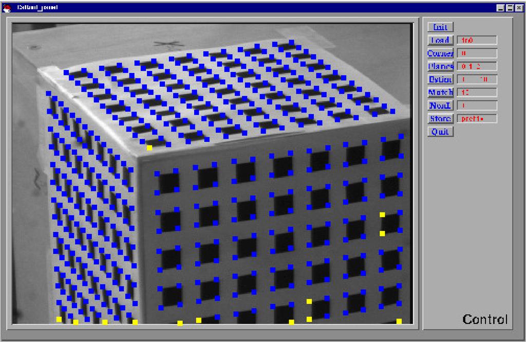
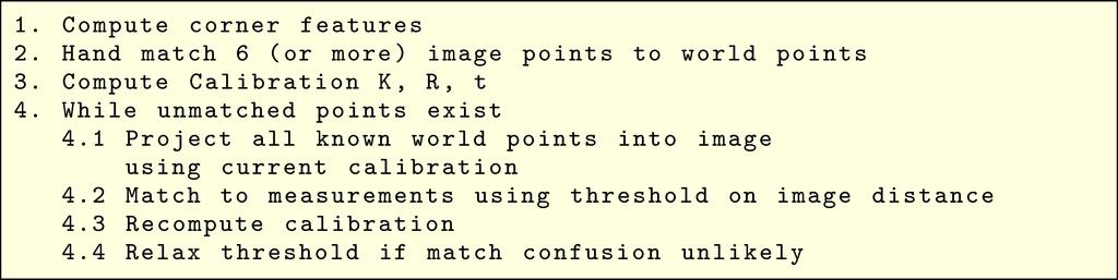
51 Camera Calibration Example Algorithm

52 Radial Distortion So far, we have figured out the transformations that turn our camera into a notional camera with the world and the camera coordinates aligned and an ideal image plane. One often has to correct for the other optical distortions and aberrations. Radial distortion is the most common see the Q sheet. Correction for this distortion is applied before carrying out calibration.

53 Practical Camera Calibration Matlab Calibration Toolkit

54 Summary of Lecture In this lecture we have: Introduced the aims of computer vision, and some paradigms. Explored linear transformations and introduced homogeneous coordinates. Defined perspective projection from a scene, and saw that it could be made linear using homogeneous coordinates. Discussed how to pre-calibrate a camera using image of six or more known scene points.