Categorical Data in a Designed Experiment Part 2: Sizing with a Binary Response

Transcription

1 Categorical Data in a Designed Experiment Part 2: Sizing with a Binary Response Authored by: Francisco Ortiz, PhD Version 2: 19 July 2018 Revised 18 October 2018 The goal of the STAT COE is to assist in developing rigorous, defensible test strategies to more effectively quantify and characterize system performance and provide information that reduces risk. This and other COE products are available at STAT Center of Excellence 2950 Hobson Way Wright-Patterson AFB, OH 45433

2 Table of Contents Introduction... 2 Background... 2 Target Location Error (TLE) Example Revisited... 2 The Binomial Distribution... 5 Method... 9 Method 1: Arcsine Transformation Approach... 9 Method 2: Signal to Noise Calculations Arcsine Formulation Logit Formulation Normal Approximation Formulation Using the signal-to-noise ratio (JMP 10 Demo) Method 3: Inverse Binomial Sampling Scheme Conclusion References Addendum (Updated July 19, 2018): Revision 1, 18 Oct 2018: Formatting and minor typographical/grammatical edits.

3 Introduction In Part 1 of this best practice series, we learned that the data type used to represent a response can affect the size of the experiment and the quality of its analysis. Categorical data types, such as binary (pass/fail) measures, contain a relatively poor amount of information in comparison to continuous data types. This reduction in information increases the number of samples needed to detect significant changes of a response in the presence of noise. The use of categorical data types for responses should be avoided; however, there will be circumstances in which a pass/fail measure is the only practical way to characterize a system s performance. Three methods to estimate the sample size needed for a designed experiment using a binary response will be presented in this paper, the arcsine transformation approach, the signal-to-noise method, and the inverse binomial sampling scheme method. The circumstances in which each method can be applied will be described in the paper. The methods will be demonstrated using a Target Location Error (TLE) example, originally presented in part 1 of this series. All methods presented are available with the Binary Response Calculator on the STAT COE website. Keywords: binary responses, categorical factors, sample size, test and evaluation, design of experiments, confidence, power Background Target Location Error (TLE) Example Revisited Let s revisit the missile targeting system example from part 1 of this best practice series. In this example, we are comparing the ability of a missile targeting system to accurately assess the coordinates of a target within a tolerance radius of 10 feet. An example of the error distribution (using notional data) is shown in Figure 1. 2

4 Y2 Axis Y1 Axis Figure 1: Distribution of error distance example (notional data) Let s assume the only way to measure the systems is to categorize each attempt as either a Pass or Fail based on whether it falls within a 10 feet radius of the target (see Figure 2). This is a type of nominal response, specifically a binary response. Figure 2: Measuring using binary (Pass/Fail) response The purpose for this test is to evaluate the performance of the system in various simulated engagements and also to determine what factors affect the probability of success. The objective and 3

5 threshold probabilities of success (P s ) for the system are 90% and 85% respectively, under all expected conditions. The test engineers have decided to vary four different factors, Altitude, Range, Aircraft Speed, and AOA. A 2 4 factorial design has been chosen to set up the simulated engagements, see the coded matrix below (-1 and 1 are the low and high-level values of a factor respectively). This design will allow the practitioner the ability to test what main effects and interactions terms significantly affect the response, the observed proportion of success (p ). Runs Table 1: 2 4 factorial design for TLE example X 1 : Altitude X 2 : Range X 3 : Aircraft Speed X 4 : AOA Consider the following graph where the response, probability of success (P s ), is graphed versus the low and high settings of X 1 (Altitude). 4

6 Figure 3: Power represents the ability to detect a difference between factor levels Power is the probability that we can detect a significant difference () between P Low and P High. The values for P Low, P Avg, P High and can be derived from the objective and threshold requirement (90% and 85%). So for this TLE example, the objective (P S ) of 90% represents the P Avg and the threshold value of 85% represents P Low, therefore P High would be 95%. Delta therefore would be (P High - P Low), 10%. The question that must now be answered is how many replicates of each design point must be run in order to achieve appropriate levels of power and confidence. Let s assume for this example that we will go with the DoD standard of 80% confidence and 80% power for a test (α = β = 0.2). In this paper, we will introduce a calculator/app that will aid practitioners in answering this question. But, before doing so, let s first discuss the distribution the data comes from, the binomial distribution. The Binomial Distribution The binomial distribution is a discrete probability distribution of the number of successes in a series of n independent Bernoulli trials (pass/fail experiments), each trial yields success with probability p. The probability mass function is defined as: n m P( Y m) p (1 p) m nm (1) for m = 1,2, n. The cumulative distribution function can be expressed as: 5

7 (2) P( Y m) P Y j If a large enough sample size, n, is used, the binomial distribution begins to look like the normal distribution and its parameters can be approximated with the following formulas. Mean: Standard Deviation: m j0 np (3) np(1 p) (4) A rule of thumb commonly used to ensure that the distribution can be approximated by the normal distribution is the rule of five : np 5 and n(1 p) 5 (5) The farther p is from 0.5 the larger n needs to be in order for this approximation to work. So, for various p s, the number of reps (n)needed are as follows: Table 2: Number of reps (n)needed versus p based on the rule of five p n The following graphs provide a visual representation of how the binomial distribution behaves with varying sample sizes, n, while keeping p at 0.1. You see that around n = 50 the shape of the histogram begins to look like the normal distribution curve. 6

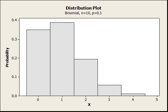
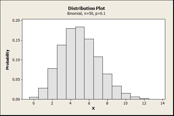
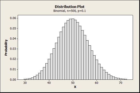
8 Figure 4: Distribution plots for p = 0. 1 for varying sample sizes, n 7

9 The following graphs provide a visual representation of how the binomial distribution behaves with varying proportions p and a constant sample size n = 100. You can see that the closer you are to the min and max values of 0 and 1 the distribution begins to looks less normal. Therefore, caution should be taken when dealing with (P s ) greater than 95% or less than 1%. 8

10 Figure 5: Distribution plots for n = 100 for varying proportions, p Method Method 1: Arcsine Transformation Approach Note that the formulation for standard deviation in equation (4) is a function of p, which is the very response we are monitoring and wish to change by varying factor levels. Due to this, the assumption of constant variance is violated. An approach to deal with this problem is to perform a variance stabilizing transformation on the observed response p. The most commonly used transformation when dealing with binomial data is the arcsine square root transformation (see equation 6). This new transformed response would be the response used in the analysis. pˆ * 1 arcsin pˆ (6) Bisgaard and Fuller (1995) use this transformation to derive the number of replicates needed when using a 2 k f factorial design with binary responses. Their formulation for the signal of interest (the change in the response we wish to detect) on the transformed scale is: arcsin p arcsin p 2 2 (7) where p is the expected proportion across the design space, and is the signal in the original scale/units. The individual point sample size is then calculated by the following formula: 9

11 2 ( z1 /2 z1 ) n (8) 2 N where z 1 α/2 and z 1 β are the critical z values based on the specified power and confidence, N is the total number of design points, and δ is defined in equation (7). To demonstrate further, let s use the TLE example introduced earlier with the Binary Response Calculator available on at the STAT COE website. The following is a screen shot of the calculator: Sample Size Calculator for Designed Experiments That Use Binary Responses User Inputs P(success) 0.8 = 0.2 Confidence 0.8 Power 0.8 k 7 f 1 Notes: - See cell comments for more details. - Inputs "k" and "f" are only needed for Methods 1 and 3. Method 1: Arcsine Transformation Approach (Bisgarrd-Fuller) Reps per run for power = 2 Reps needed for approximation 25 Recommended Units per run; n = 25 Total units = 1600 Notes: - This approach should only be used if a 2^(k-f) design is used. - See cell comments for more details. - See Bisgarrd-Fuller, 1995 for details on calculations. Method 2: Signal to Noise Calculations Signal to Noise (Arcsin method) Signal to Noise (Logit method) Signal to Noise (Normal method) Notes: - Approach can be used with any design - "Normal method" tends to be the most conservative estimated and is therefore recommended. -See "Using Method 2" tab for step by step instructions on how to use this with JMP You should still use the "Rule of 5" (see Cell C14) number if it is greater than the reps suggested by the statistical software. recommends. Method 3: Inverse Binomial Sampling Scheme (Bisgaard-Gertsbakh) Stopping rule 2 Expected n (if no change) 10 Expected n (if negative change) 5 Expected Total Units (if no change) 640 Notes: - This approach should only be used if a 2^(k-f) design is used. - Run reps until the number of failures meets the stopping rule. Record number of reps it took to get there as the response. - See cell comments for more details. - See Bisgarrd-Gertsbakh (2000) for details on calculations. Figure 6: Sample size calculator for binary responses screenshot The calculator consists of 4 sections. The User Input section, this is where the basic information about the test needs to be specified. 10

12 Figure 7: User input section The following information must be specified in this section: P(success): The expected probability of success across the design space Δ: The signal of interest (the change in the response we wish to detect) Alpha: Allowable Type I error, Confidence is 1-Alpha Power: The probability of detecting Δ, 1-Power is the Type II error k: The number of factors in the design (4 in this case) f: The level we wish to fractionate the factorial (0 in this case since this is a full factorial) Remember, for our example, the objective and threshold P s for the system are 90% and 85% respectively. Therefore, P(success) is set to 0.9 and Δ is equal to 0.1. We re going with the DoD standard of 80% confidence and 80% power for a test (α = β = 0.2). We are using a 2 4 full factorial design so k = 4 and f = 0. The Method 1 section displays the results from applying the approach defined by Bisgaard and Fuller (1995). Figure 8: Method 1- Arcsine Transformation Approach The following describes the output: Reps per run for power: Based on equation (8) Reps needed for approximation: Based on the rule of 5 11

13 Recommended Units per run: Takes the maximum value between the reps needed for power and the reps needed for the approximation Total units: The total number of runs times the recommended number of reps For the TLE example, the calculator is recommending 50 reps for each of the 2 4 = 16 design points, resulting in a total of 800 runs. Method 2: Signal to Noise Calculations Method 1, the Arcsine Transformation Approach, only works if a 2 k f designs is used. If another type of design is used, a better approach would be to use the signal-to-noise ratio (SNR) method. The signal to noise ratio is simply the ratio between the measured change in the response we wish to detect (δ, the signal of interest) and the estimated standard deviation of the system (noise). See the formula below: SNR (9) Three methods of calculating the SNR are presented in the calculator. Method 2: Signal to Noise Calculations Signal to Noise (Arcsin method) Signal to Noise (Logit method) Signal to Noise (Normal method) Figure 9: Method 2- Signal to Noise Calculations Arcsine Formulation This method uses the same formulations for delta and sigma that were derived in the Bisgaard and Fuller (1995) paper. Delta (in the transformed scale) is the same as in equation (7) repeated here for convenience: 1 arcsin p arcsin p 2 2 The standard deviation for the arcsine transformation is as follows: 12

14 1 1 1 (10) 4n 2 where n = 1 here since we wish to determine what the SNR is before replication. Logit Formulation This approach uses the Logit transformation, which is the traditional solution used when applying logistic regression to fit a model where the dependent variable is a proportion. The transformation takes the log of the odds: pˆ * 2 pˆ ln 1 pˆ (11) where p is the probability of an event occurring, 1 p is the probability of an event not occurring, and p 1 p is the odds of the event. Delta in the transformed scale is defined below: 2 p 1 p 2 ln ln 1 p 1 p 1 2 (12) where p 1 p and p2 2 p. The standard deviation is defined as follows: 2 2 np(1 p) p(1 p) (13) where n = 1 here, since we wish to determine what the SNR is before replication. Normal Approximation Formulation The final SNR formulation is based on the Normal Approximation of the binomial. This is the simplest of the formulations presented in this paper. Delta is defined as: p p (14) where p 1 p and p2 2 in equation 13: p. The standard deviation is defined the same as the logit formulation 2 3 np(1 p) p(1 p) 13

15 where n = 1 here, since we wish to determine what the SNR is before replication. Figure 9 shows the results from the calculator using the TLE Example. Note that all three methods provide similar results. Table 3 shows the SNR results of the three methods when varying p. The Normal Approximation method consistently produces the most conservative estimate of the SNR. Table 3: Comparison of SNR calculation methods p SNR (arcsin) SNR (logit) SNR (normal) Using the signal-to-noise ratio (JMP 10 Demo) Most design of experiments (DOE) software will allow you to input the SNR in order to calculate the power of the test. In this section, we will demonstrate how to use the SNR with JMP 10. Step 1: Create your design in JMP Create a 2 4 factorial design to match our TLE example. The columns X1, X2, X3, X4 columns represent our factors Altitude, Range, Aircraft Speed, AOA respectively. The Y column is our pass/fail response. 14

16 Step 2: Evaluate design Once the design is created, select DOE > Evaluate Design. 15

17 Specify the response and factor columns and then click OK. The Evaluate Design dialog box will appear. In the Evaluate Design dialog box: o Specify the terms in your model. For this example, we are interested in main effects and two factor interactions. o Set significance level at α = 0.2. o Input SNR from the calculator. 16

18 Note: Power is 28% for all terms if we only run each setting once. 17

19 Step 3: Augment design Augment the design to add replicates and bring power up to appropriate level. For this example, we want 80%. Select DOE > Augment Design. Specify the response and factor columns and then click OK. The Augment Design dialog box will appear. 18

20 Make sure all factors to be replicated are listed. Click the replicate button. Enter the number of times to replicate each design point. Check the Power Analysis section of the resulting design. Confirm that calculations are above or close to predetermined power objectives. In this case, 80%. If not, click the back button and increase the number of replicates until you achieve your power objective. Method 3: Inverse Binomial Sampling Scheme The final method provided by the calculator is the Inverse Binomial Sampling Scheme proposed in Bisgaard and Gertsbakh (2000). This method can be used with a 2 k f design where the purpose is to reduce the rate of defectives. Instead of determining a fixed sample size for each design run, this approach suggests sampling until a fixed number of defects r, are observed. The derivation for the stopping rule will not be covered in this paper, for more details please refer to Bisgaard and Gertsbakh (2000). The number of defects observed, r, is based on the number of factorial trials in a 2 k f design, 19

21 the change in probability to detect Δ, and the fixed levels of α and β. The total number of reps until r defects occurs is used as the response. This approach could significantly reduce the number of total runs needed if the system does not meet the P s requirement. Figure 10: Inverse Binomial Sampling Scheme output The following describes the calculator s output: Stopping rule: The number of defects to observe for each design run Expected n (if no change): Based on the estimated P s, this is the expected number of reps needed to observe the stopping rule Expected n (if negative change): If a negative change of Δ has occurred, this is the expected number of reps needed to observe the stopping rule Note that an unequal number of reps for each design run is likely; therefore, a general linear model (GLM) or weighted least squares (WLS) approach is recommended for the analysis. Conclusion Three methods to estimate the samples size needed for a designed experiment using binary responses were presented in this paper. The arcsine transformation approach can be used if a 2 k f design is employed. The signal-to-noise method can be used for any design but requires iterative exploration of the number of replicates needed using statistical software. A JMP 10 tutorial on how to do this was provided. The Inverse Binomial Sampling Scheme method can also be used if a 2 k f design is employed. This method could be a potential resource saving approach for system with a high expected probability of success (P s ), and if the goal is to simply demonstrate that the system meets that objective P s. All methods presented are available for use on the Binary Response Calculator available on at the STAT COE website. There are opportunities for future work on this subject. A Monte Carlo approach should be considered in order to produce more accurate power calculations that are robust to the experimental design used. Also, future research should explore the use of OC curves and sequential probability ratio testing in order to truncate and quickly stop testing if it is abundantly clear that the system is passing or failing the requirements. 20

22 References Bisgaard, Søren, and Howard T. Fuller. Sample Size Estimates for 2k-p Designs with Binary Responses. Journal of Quality Technology, vol. 27, no. 4, 1995, pp , doi: / Bisgaard, Søren, and Ilya Gertsbakh. 2k- Experiments with Binary Responses: Inverse Binomial Sampling. Journal of Quality Technology, vol. 32, no. 2, 2000, pp , doi: / Gotwalt, C., JMP Script for Computing Binary Power using the Logit Transformation, JMP, Lenth, Russ. Java Applets for Power and Sample Size. Retrieved 2014 from Whitcomb, Pat, and Mark Anderson. Excel Sample Size Calculator for Binary Responses. Stat-Ease,

23 SNR STAT COE-Report Addendum (Updated July 19, 2018): The STAT COE has created a new calculator to help estimate signal-to-noise for a binary response. The new tool allows a practitioner to evaluate the effects of increasing the number of replicates for each test design point to the signal-to-noise ratio (SNR). The following is a brief tutorial on how to use the new tool. Signal-to-Noise Estimator for a Binary Response Inputs Values Output Table 1: Ps(Avg) 0.9 P s(low) 0.85 Reps Normal Arcsin Logit Avg. Reps 1 User Specified Calculations Values P s (High) P s (Low) = Output Table 2: Replicates Normal Arcsin Logit Average Reps Normal Arcsin Logit Average Figure 11: SNR estimator for a binary response Recall our TLE Example, where the objective and threshold probability of success (P s ) for the system is 90% and 85% respectively, under all expected conditions. The following graph shows the response, probability of success (P s ), versus the low and high settings of a factor X 1. 22

24 Figure 12: Power represents the ability to detect a difference between factor levels The values for P Low, P Avg, P High, and can be derived from the objective and threshold requirement. P Avg is our objective value 90%, P Low is 85%, P High would be 95%, and therefore is 10%. In the input section, we would enter the following information: Inputs Values P s (Avg) 0.9 P s (Low) 0.85 Reps 1 The calculation section would display the following: Figure 13: SNR calculator inputs Calculations Values P s (High) 0.95 P s (Low) 0.85 = 0.1 Figure 14: SNR calculations for P Low, P High, and 23

25 The Output Table 1 shows what the estimated signal-to-noise would be using the three formulations described in this paper (Normal, Arcsine, and Logit). The first row shows the estimates based on the number of reps entered in the inputs sections. The following rows show how the SNR changes for differing numbers of reps (1, 5, 10, etc.). Output Table 1: Reps Normal Arcsin Logit Avg. User Specified Figure 15: Output Table 1, summary of the effects of reps to SNR Output Table 2, shows a finer or more detailed analysis of the effect replicates have on the SNR estimates. Output Table 2: Replicates Normal Arcsin Logit Average Figure 16: Output Table 2, detailed report of the effects of reps to SNR A graphical representation of the results is also provided. 24

26 Figure 17: Graphical representation of SNR estimation results In practice, a SNR of about 2 is usually a good target to aim for when it comes to SNR. This means that results that are 2 sigma away from what should be expected will be flag as significant in your analysis. In this case you see that 40 reps produce an average SNR of In Output Table 2, we get a more precise value of 34 reps. The next step is to create a test design and use the estimated SNR to calculate power and confidence. In our example, a 2 4 design with 40 reps will produce the following power numbers: 25

27 Figure 18: Power calculations based on SNR estimate All terms are well above 80% with 95% confidence and satisfy the DoD standard of 80% confidence and 80% power. 26