OLC Wasco County: Delivery One.

Transcription

1 OLC Wasco County: Delivery One January 2, 2014

2 Trimble R7 Receiver set up over GPS monument WASCO_02. Data collected for: Oregon Department of Geology and Mineral Industries 800 NE Oregon Street Suite 965 Portland, OR Prepared by: WSI, A Quantum Spatial Company 421 SW 6th Avenue Suite 800 Portland, Oregon phone: (503) fax: (503) SW 2nd Street Suite 400 Corvallis, OR phone: (541) fax: (541) ii

3 Contents 2 - Project Overview 3 - Aerial Acquisition 3 - LiDAR Survey 4 - Ground Survey 4 - Instrumentation 4 - Monumentation 6 - Methodology 7 - LiDAR Accuracy 7 - Relative Accuracy 8 - Vertical Accuracy 9 - Density 9 - Pulse Density 10 - Ground Density 12 - Appendix A : PLS Certification 13 - Appendix B : GPS Monument Table 1

4 Overview Project Overview WSI has completed the acquisition and processing of Light Detection and Ranging (LiDAR) data for the OLC Wasco County Delivery Area One for the Oregon Department of Geology and Mineral Industries (DOGAMI). The Oregon LiDAR Consortium s Wasco County 2014 project area of interest (AOI) encompasses 1,020,680 acres. Delivery Area One encompasses 176,896.6 acres. The collection of high resolution geographic data is part of an ongoing pursuit to amass a library of information accessible to government agencies as well as the general public. OLC Wasco County Delivery One Data Delivered: January 2, 2014 Acquisition Dates 7/15/2014-9/19/2014 Delivery Area One Area of Interest 176,896.6 acres Projection Oregon Statewide Lambert (OGIC) Datum: horizontal & vertical Units NAD83 (2011) NAVD88 (Geoid 12A) International Feet WSI LiDAR data acquisition occurred from July 15 - September 19, Study Area Settings for LiDAR data capture produced an average resolution of at least eight pulses per square meter. Final products created that are included in Delivery Area One are LiDAR point cloud data, three-foot digital elevation models of bare earth ground models and highest-hit returns, 1.5-foot intensity rasters, three-foot ground density rasters, study area vector shapes, ground survey points and monuments, and corresponding statistical data. WSI acquires and processes data in the most current, NGS-approved datums and geoid. For OLC Wasco County, all final deliverables are projected in Oregon Statewide Lambert, endorsed by the Oregon Geographic Information Council (OGIC), 1 using the NAD83(2011) horizontal datum and the NAVD88 (Geoid 12A) vertical datum, with units in international feet. 1 coordination/projections/projections.aspx 2

5 Aerial Acquisition Aerial Acquisition LiDAR Survey The LiDAR survey used a Leica ALS70 and an Optech Orion H sensor mounted in a Cessna U206G, Partenavia P.68, and Piper Navajo. The systems were programmed to emit single pulses at a rate of 219 kilohertz and flown between 600 and 1,600 meters above ground level (AGL), capturing a scan angle of +/-15 degrees from nadir (field of view equal to 30 degrees). These settings are developed to yield points with an average native density of greater than eight pulses per square meter over terrestrial surfaces. Project Flightlines The native pulse density is the number of pulses emitted by the LiDAR system. Some types of surfaces such as dense vegetation or water may return fewer pulses than the laser originally emitted. Therefore, the delivered density can be less than the native density and lightly vary according to distributions of terrain, land cover, and water bodies. The study area was surveyed with opposing flight line side-lap of greater than 60 percent with at least 100 percent overlap to reduce laser shadowing and increase surface laser painting. The system allows up to four range measurements per pulse, and all discernible laser returns were processed for the output dataset. To solve for laser point position, it is vital to have an accurate description of aircraft position and attitude. Aircraft position is described as x, y, and z and measured twice per second (two hertz) by an onboard differential GPS unit. Aircraft attitude is measured 200 times per second (200 hertz) as pitch, roll, and yaw (heading) from an onboard inertial measurement unit (IMU). As illustrated in the accompanying map, 413 flightlines provide coverage of the study area ,600 m AGL 30 OLC Wasco County LiDAR Acquisition Specifications Sensors Deployed Leica ALS 70 and Orion H Aircraft Cessna U206G, Piper Navajo, Partenavia P.68 Survey Altitude (AGL) 600-1,600 meters Pulse Rate 219 khz Pulse Mode Single (SPiA) Field of View (FOV) 30 Roll Compensated Yes Overlap 100% overlap with 60% sidelap Pulse Emission Density 8 pulses per square meter 3

6 Ground Survey Ground Survey Ground control surveys, including monumentation, aerial targets, and ground check points (GCPs) were conducted to support the airborne acquisition. Ground control data are used to geospatially correct the aircraft positional coordinate data and to perform quality assurance checks on final LiDAR data products. See the table to the right for specifications of equipment used. Instrumentation All Global Navigation Satellite System (GNSS) static surveys utilized Trimble R7 GNSS receivers with Zephyr Geodetic Model 2 RoHS antennas and Trimble R8 GNSS receivers with internal antennas. Rover surveys for GCP collection were conducted with Trimble R6, Trimble R8, and Trimble R10 GNSS receivers. Monumentation Existing and newly established survey benchmarks serve as control points during LiDAR acquisition. Monument locations were selected with consideration for satellite visibility, field crew safety, and optimal location for GCP coverage. NGS benchmarks are preferred for control points; however, in the absence of NGS benchmarks, WSI produces our own monuments, and every effort is made to keep them within the public right of way or on public lands. If monuments are necessary on private property, consent from the owner is required. All monumentation is done with 5/8 x 30 rebar topped with a two-inch diameter aluminum cap stamped Watershed Sciences, Inc. Control. The table at right provides the list of monuments used in Delivery Area One. See Appendix B for a complete list of monuments placed within the OLC Wasco County 2014 Study Area. Receiver Model Trimble R7 GNSS Trimble R8 Instrumentation Antenna OPUS Antenna ID Use Zephyr GNSS Geodetic Model 2 RoHS Integrated Antenna R8 Model 2 TRM TRM_R8_GNSS Delivery Area One GPS Monuments Ellipsoid PID Latitude Longitude Height (m) Static Static, Rover Trimble R10 Integrated Antenna R10 TRMR10 Rover Trimble R6 Integrated Antenna R10 TRMR10 Rover WASCO_ ' " ' " WASCO_ ' " ' " NAVD88 Height (m) WASCO_ ' " ' " WASCO_ ' " ' " WASCO_ ' " ' " WASCO_ ' " ' " WASCO_ ' " ' " WASCO_ ' " ' " Coordinates are on the NAD83 (2011) datum, epoch NAVD88 height referenced to Geoid12A. GPS receiver set over GPS Monument WASCO_07. 4

7 Ground Survey 5

8 Ground Survey Methodology To correct the continuously recorded aircraft position, WSI concurrently conducts multiple static GNSS ground surveys over each monument. All control monuments are observed for a minimum of two survey sessions, each lasting no fewer than two hours. Data are collected at a rate of one hertz, using a 10 degree mask on the antenna. The static GPS data are then triangulated with nearby Continuously Operating Reference Stations (CORS) using the Online Positioning User Service (OPUS ) for precise positioning. Ground Check Points (GCPs) are collected using Real Time Kinematic (RTK), Post-Processed Kinematic (PPK), and Fast-Static (FS) survey techniques. For RTK surveys, a base receiver is positioned at a nearby monument to broadcast a kinematic correction to a roving receiver; for PPK and FS surveys, however, these corrections are post-processed. All GCP measurements are made during periods with a Position Dilution of Precision (PDOP) no greater than 3.0 and in view of at least six satellites for both receivers. Relative errors for the position must be less than 1.5 centimeters horizontal and 2.0 centimeters vertical in order to be accepted. In order to facilitate comparisons with high quality LiDAR data, GCP measurements are not taken on highly reflective surfaces such as center line stripes or lane markings on roads. GCPs are taken no closer than one meter to any nearby terrain breaks such as road edges or drop offs. GCPs were collected within as many flight lines as possible; however, the distribution depended on ground access constraints and may not be equitably distributed throughout the study area. Monument Accuracy FGDC-STD Rating St Dev NE 0.05 m Horizonta St Dev z 0.05 m Vertical WSI ground professional collecting ground survey points in OLC Wasco County study area. Ground professional collecting RTK 6

9 Accuracy LiDAR Accuracy Relative Accuracy Relative accuracy refers to the internal consistency of the data set and is measured as the divergence between points from different flightlines within an overlapping area. Divergence is most apparent when flightlines are opposing. When the LiDAR system is well calibrated the line to line divergence is low (<10 centimeters). Internal consistency is affected by system attitude offsets (pitch, roll, and heading), mirror flex (scale), and GPS/IMU drift. Relative Accuracy Calibration Results N = 962 flightlines Project Average 0.11 ft. (0.03 m) Median Relative Accuracy 0.11 ft. (0.03 m) 1σ Relative Accuracy 0.12 ft. (0.04 m) 2σ Relative Accuracy 0.15 ft. (0.04 m) Relative accuracy statistics are based on the comparison of 962 full and partial flightlines. Relative accuracy is reported for the cumulative delivered portions of the study area. Relative Accuracy Distribution 40% 35% 962 Flightlines Relative Accuracy Distribution 30% 25% 20% 15% 10% 5% 0% Relative Accuracy (ft) Total Compared Points (n = 59,838,676,207 ) R7 Receiver 7

10 Accuracy Vertical Accuracy Vertical Accuracy reporting is designed to meet guidelines presented in the National Standard for Spatial Data Accuracy (NSSDA) (FGDC, 1998) and the ASPRS Guidelines for Vertical Accuracy Reporting for LiDAR Data V1.0 (ASPRS, 2004). The statistical model compares known ground check points to the triangulated LiDAR surface. Vertical accuracy statistical analysis uses ground control points in open areas where the LiDAR system has a very high probability that the sensor will measure the ground surface and is evaluated at the 95th percentile. For the OLC Wasco County 2014 Delivery Area One, 6,295 GCPs were collected. Statistics are shown for Delivery Area One. For this project, no independent survey data were collected, nor were reserved points collected for testing. As such, vertical accuracy statistics are reported as Compiled to Meet. Vertical Accuracy is reported for the entire study area and reported in the table below. Histogram and absolute deviation statistics displayed below. Sample Size (n) Vertical Accuracy Results Delivery Area One 6,295 Ground check points Root Mean Square Error 0.09 ft. (0.03 m) 1 Standard Deviation 0.15 ft. (0.05 m) 2 Standard Deviation 0.27 ft. (0.08 m) Average Deviation 0.12 ft. (0.04 m) Minimum Deviation ft. (-0.09 m) Maximum Deviation 0.56 ft. (0.17 m) Vertical Accuracy Distribution GCP Absolute Error 100% Absolute Error: Laser point to GCP Deviation 60% 90% 80% 0.60 RMSE 1 Sigma 2 Sigma Absolute Error Distribution 40% 20% 70% 60% 50% 40% 30% 20% 10% Cumulative Distribution Absolute Error (feet) % 0% Deviation ~ Laser Point to Nearest Ground Survey Point (feet) Ground Survey Point 8

11 Density Density Pulse Density Final pulse density is calculated after processing and is a measure of first returns per sampled area. Some types of surfaces (e.g., dense vegetation, water) may return fewer pulses than the laser originally emitted. Therefore, the delivered density can be less than the native density and vary according to terrain, land cover, and water bodies. Density histograms and maps have been calculated based on first return laser pulse density and ground-classified laser point density. Densities are reported for the delivery area. Average Pulse Density pulses per square meter pulses per square foot Average Pulse Density per 0.75 USGS Quad (color scheme aligns with density chart). 40% 30% Percent Distribution 20% 10% 0% Pulses per Square Foot 9

12 Density Ground Density Ground classifications were derived from ground surface modeling. Further classifications were performed by reseeding of the ground model where it was determined that the ground model failed, usually under dense vegetation and/or at breaks in terrain, steep slopes, and at tile boundaries. The classifications are influenced by terrain and grounding parameters that are adjusted for the dataset. The reported ground density is a measure of ground-classified point data for the delivery area. Ground Density points per square meter points per square foot Average Ground Density per 0.75 USGS Quad (color scheme aligns with density chart). 40% 30% Percent Distribution 20% 10% 0% Ground Points per Square Foot 10

13 Appendix [ Page Intentionally Blank ] 11

14 Appendix A : PLS Certification Appendix 12/31/

15 Appendix B : GPS Monument Table Appendix List of GPS monuments used in OLC Wasco County Survey Area. Coordinates are on the NAD83 (2011) datum, epoch NAVD88 height referenced to Geoid12A. OLC Wasco County GPS Monuments PID Latitude Longitude Ellipsoid Height (m) Orthometric Height (m) RC ' " ' " RC ' " ' " WASCO_ ' " ' " WASCO_ ' " ' " WASCO_ ' " ' " WASCO_ ' " ' " WASCO_ ' " ' " WASCO_ ' " ' " WASCO_ ' " ' " WASCO_ ' " ' " WASCO_ ' " ' " WASCO_ ' " ' " WASCO_ ' " ' " WASCO_ ' " ' " WASCO_ ' " ' " WASCO_ ' " ' " WASCO_ ' " ' " WASCO_ ' " ' " WASCO_ ' " ' " WASCO_ ' " ' " WASCO_ ' " ' " WASCO_ ' " ' " WASCO_ ' " ' " WASCO_ ' " ' "

16 Appendix OLC Wasco County GPS Monuments PID Latitude Longitude Ellipsoid Height (m) Orthometric Height (m) WASCO_ ' " ' " WASCO_ ' " ' " WASCO_ ' " ' " WASCO_ ' " ' " WASCO_ ' " ' " WASCO_ ' " ' " WASCO_ ' " ' " WASCO_ ' " ' " WASCO_ ' " ' " WASCO_ ' " ' " WASCO_ ' " ' " WASCO_ ' " ' " WASCO_ ' " ' " WASCO_ ' " ' " WASCO_ ' " ' " WASCO_ ' " ' " WASCO_ ' " ' "

17 OLC Wasco County: Delivery Two January 23, 2015

18 Trimble R7 Receiver set up over GPS monument WASCO_03. Data collected for: Oregon Department of Geology and Mineral Industries 800 NE Oregon Street Suite 965 Portland, OR Prepared by: WSI, A Quantum Spatial Company 421 SW 6th Avenue Suite 800 Portland, Oregon phone: (503) fax: (503) SW 2nd Street Suite 400 Corvallis, OR phone: (541) fax: (541) ii

19 Contents 2 - Project Overview 3 - Aerial Acquisition 3 - LiDAR Survey 4 - Ground Survey 4 - Instrumentation 4 - Monumentation 6 - Methodology 7 - LiDAR Accuracy 7 - Relative Accuracy 8 - Vertical Accuracy 9 - Density 9 - Pulse Density 10 - Ground Density 12 - Appendix A : PLS Certification 13 - Appendix B : GPS Monument Table 1

20 Overview Project Overview WSI has completed the acquisition and processing of Light Detection and Ranging (LiDAR) data for the OLC Wasco County Delivery Area Two for the Oregon Department of Geology and Mineral Industries (DOGAMI). The Oregon LiDAR Consortium s Wasco County 2014 project area of interest (AOI) encompasses 1,020,680 acres. Delivery Area Two encompasses 248,832 acres. OLC Wasco County Delivery Two Data Delivered: January 2, 2014 Acquisition Dates 8/2/2014-9/16/2014 Delivery Area Two Area of Interest 248,832 acres Projection Oregon Statewide Lambert (OGIC) Datum: horizontal & vertical NAD83 (2011) NAVD88 (Geoid 12A) The collection of high resolution geographic data is part of an ongoing pursuit to amass a library of information accessible to government agencies as well as the general public. Units International Feet WSI LiDAR data acquisition occurred from July 15 - September 19, Study Area Settings for LiDAR data capture produced an average resolution of at least eight pulses per square meter. Final products created that are included in Delivery Area Two are LiDAR point cloud data, three-foot digital elevation models of bare earth ground models and highest-hit returns, 1.5-foot intensity rasters, three-foot ground density rasters, study area vector shapes, ground survey points and monuments, and corresponding statistical data. WSI acquires and processes data in the most current, NGS-approved datums and geoid. For OLC Wasco County, all final deliverables are projected in Oregon Statewide Lambert, endorsed by the Oregon Geographic Information Council (OGIC), 1 using the NAD83(2011) horizontal datum and the NAVD88 (Geoid 12A) vertical datum, with units in international feet. 1 coordination/projections/projections.aspx 2

21 Aerial Acquisition Aerial Acquisition LiDAR Survey The LiDAR survey used a Leica ALS70 and an Optech Orion H sensor mounted in a Cessna U206G, Partenavia P.68, and Piper Navajo. The systems were programmed to emit single pulses at a rate of 219 kilohertz and flown between 600 and 1,600 meters above ground level (AGL), capturing a scan angle of +/-15 degrees from nadir (field of view equal to 30 degrees). These settings are developed to yield points with an average native density of greater than eight pulses per square meter over terrestrial surfaces. Project Flightlines The native pulse density is the number of pulses emitted by the LiDAR system. Some types of surfaces such as dense vegetation or water may return fewer pulses than the laser originally emitted. Therefore, the delivered density can be less than the native density and lightly vary according to distributions of terrain, land cover, and water bodies. The study area was surveyed with opposing flight line side-lap of greater than 60 percent with at least 100 percent overlap to reduce laser shadowing and increase surface laser painting. The system allows up to four range measurements per pulse, and all discernible laser returns were processed for the output dataset. To solve for laser point position, it is vital to have an accurate description of aircraft position and attitude. Aircraft position is described as x, y, and z and measured twice per second (two hertz) by an onboard differential GPS unit. Aircraft attitude is measured 200 times per second (200 hertz) as pitch, roll, and yaw (heading) from an onboard inertial measurement unit (IMU). As illustrated in the accompanying map, 522 full and partial flightlines provide coverage of the study area ,600 m AGL 30 OLC Wasco County LiDAR Acquisition Specifications Sensors Deployed Leica ALS 70 and Optech Orion H Aircraft Cessna U206G, Piper Navajo, Partenavia P.68 Survey Altitude (AGL) 600-1,600 meters Pulse Rate 219 khz Pulse Mode Single (SPiA) Field of View (FOV) 30 Roll Compensated Yes Overlap 100% overlap with 60% sidelap Pulse Emission Density 8 pulses per square meter 3

22 Ground Survey Ground Survey Ground control surveys, including monumentation, aerial targets, and ground survey points (GSPs) were conducted to support the airborne acquisition. Ground control data are used to geospatially correct the aircraft positional coordinate data and to perform quality assurance checks on final LiDAR data products. See the table to the right for specifications of equipment used. Instrumentation All Global Navigation Satellite System (GNSS) static surveys utilized Trimble R7 GNSS receivers with Zephyr Geodetic Model 2 RoHS antennas and Trimble R8 GNSS receivers with internal antennas. Rover surveys for GSP collection were conducted with Trimble R6, Trimble R8, and Trimble R10 GNSS receivers. Monumentation Existing and newly established survey benchmarks serve as control points during LiDAR acquisition. Monument locations were selected with consideration for satellite visibility, field crew safety, and optimal location for GSP coverage. NGS benchmarks are preferred for control points; however, in the absence of NGS benchmarks, WSI produces our own monuments, and every effort is made to keep them within the public right of way or on public lands. If monuments are necessary on private property, consent from the owner is required. All monumentation is done with 5/8 x 30 rebar topped with a two-inch diameter aluminum cap stamped Watershed Sciences, Inc. Control. The table at right provides the list of monuments used in Delivery Area Two. See Appendix B for a complete list of monuments placed within the OLC Wasco County 2014 Study Area. Receiver Model Trimble R7 GNSS Trimble R8 Instrumentation Antenna OPUS Antenna ID Use Zephyr GNSS Geodetic Model 2 RoHS Integrated Antenna R8 Model 2 TRM TRM_R8_GNSS Delivery Area Two GPS Monuments Ellipsoid PID Latitude Longitude Height (m) Static Static, Rover Trimble R10 Integrated Antenna R10 TRMR10 Rover Trimble R6 Integrated Antenna R6 TRMR6 Rover NAVD88 Height (m) RC ' " ' " WASCO_ ' " ' " WASCO_ ' " ' " WASCO_ ' " ' " WASCO_ ' " ' " WASCO_ ' " ' " WASCO_ ' " ' " WASCO_ ' " ' " WASCO_ ' " ' " WASCO_ ' " ' " WASCO_ ' " ' " WASCO_ ' " ' " Coordinates are on the NAD83 (2011) datum, epoch NAVD88 height referenced to Geoid12A. 4

23 Ground Survey 5

24 Ground Survey Methodology To correct the continuously recorded aircraft position, WSI concurrently conducts multiple static GNSS ground surveys over each monument. All control monuments are observed for a minimum of two survey sessions, each lasting no fewer than two hours. Data are collected at a rate of one hertz, using a 10 degree mask on the antenna. The static GPS data are then triangulated with nearby Continuously Operating Reference Stations (CORS) using the Online Positioning User Service (OPUS ) for precise positioning. Ground Survey Points (GSPs) are collected using Real Time Kinematic (RTK), Post-Processed Kinematic (PPK), and Fast- Static (FS) survey techniques. For RTK surveys, a base receiver is positioned at a nearby monument to broadcast a kinematic correction to a roving receiver; for PPK and FS surveys, however, these corrections are post-processed. All GSP measurements are made during periods with a Position Dilution of Precision (PDOP) no greater than 3.0 and in view of at least six satellites for both receivers. Relative errors for the position must be less than 1.5 centimeters horizontal and 2.0 centimeters vertical in order to be accepted. In order to facilitate comparisons with high quality LiDAR data, GSP measurements are not taken on highly reflective surfaces such as center line stripes or lane markings on roads. GSPs are taken no closer than one meter to any nearby terrain breaks such as road edges or drop offs. GSPs were collected within as many flight lines as possible; however, the distribution depended on ground access constraints and may not be equitably distributed throughout the study area. Monument Accuracy FGDC-STD Rating St Dev NE St Dev z 0.05 m Horiz 0.05 m Vert WSI ground professional collecting ground survey points in OLC Wasco County study area. Ground professional collecting RTK 6

25 Accuracy Results Accuracy Assessment In some cases statistics were generated for larger areas than the extent represented by delivered areas. Accuracy statistics are a product of calibration and data QA/QC methodology that are spatially coincident with production workflow, which at times exceeds the areal extent of delivery workflow. Relative Accuracy Relative accuracy refers to the internal consistency of the data set and is measured as the divergence between points from different flightlines within an overlapping area. Divergence is most apparent when flightlines are opposing. When the LiDAR system is well calibrated the line to line divergence is low (<10 centimeters). Internal consistency is affected by system attitude offsets (pitch, roll, and heading), mirror flex (scale), and GPS/IMU drift. Relative accuracy statistics are based on the comparison of 1490 full and partial flightlines. Relative accuracy is reported for the cumulative delivered portions of the study area. Relative Accuracy Calibration Results N = 1490 flightlines Project Average 0.12 ft. (0.04 m) Median Relative Accuracy 0.12 ft. (0.04 m) 1σ Relative Accuracy 0.12 ft. (0.04 m) Relative Accuracy Distribution Relative Accuracy Distribution 40% 35% 30% 25% 20% 15% 10% 5% 1490 Flightlines 0% Relative Accuracy (ft) Total Compared Points (n = 128,790,739,492 ) 2σ Relative Accuracy 0.15 ft. (0.05 m) 7

26 Accuracy Vertical Accuracy Vertical Accuracy reporting is designed to meet guidelines presented in the National Standard for Spatial Data Accuracy (NSSDA) (FGDC, 1998) and the ASPRS Guidelines for Vertical Accuracy Reporting for LiDAR Data V1.0 (ASPRS, 2004). The statistical model compares known ground survey points to the triangulated LiDAR surface. Vertical accuracy statistical analysis uses ground survey points in open areas where the LiDAR system has a very high probability that the sensor will measure the ground surface and is evaluated at the 95th percentile. For the OLC Wasco County 2014 Study area, 5,423 GSPs were used to calibrate Delivery Area Two. Statistics are shown for the cumulative delivered areas. For this project, no independent survey data were collected, nor were reserved points collected for testing. As such, vertical accuracy statistics are reported as Compiled to Meet. Vertical Accuracy is reported for the entire delivered study area and reported in the table below. Histogram and absolute deviation statistics displayed below. Sample Size (n) (ground survey points) Vertical Accuracy Results Delivery Area Two Cumulative 5,423 9,345 Root Mean Square Error 0.09 ft. (0.03 m) 0.10 ft. (0.03 m) 1 Standard Deviation 0.13 ft. (0.04 m) 0.14 ft. (0.04 m) 2 Standard Deviation 0.25 ft. (0.08 m) 0.26 ft. (0.08 m) Average Deviation 0.10 ft. (0.03 m) 0.11 ft. (0.03 m) Minimum Deviation ft. (-0.11 m) ft. (-0.11 m) Maximum Deviation 0.50 ft. (0.15 m) 0.56 ft. (0.17 m) Vertical Accuracy Distribution GSP Absolute Error Distribution 60% 55% 50% 45% 40% 35% 30% 25% 20% 15% 10% 5% 0% Deviation ~ Laser Point to Nearest Ground Survey Point (feet) 100% 90% 80% 70% 60% 50% 40% 30% 20% 10% 0% Cumulative Distribution Absolute Error (feet) Absolute Error: Laser point to GSP Deviation RMSE 1 Sigma 2 Sigma Absolute Error Ground Survey Point 8

27 Density Density Pulse Density Final pulse density is calculated after processing and is a measure of first returns per sampled area. Some types of surfaces (e.g., dense vegetation, water) may return fewer pulses than the laser originally emitted. Therefore, the delivered density can be less than the native density and vary according to terrain, land cover, and water bodies. Density histograms and maps have been calculated based on first return laser pulse density and ground-classified laser point density. Densities are reported for the delivery area. Average Pulse Density pulses per square meter pulses per square foot Average Pulse Density per 0.75 USGS Quad (color scheme aligns with density chart). 50% 40% Percent Distribution 30% 20% 10% 0% Pulses per Square Foot 9

28 Density Ground Density Ground classifications were derived from ground surface modeling. Further classifications were performed by reseeding of the ground model where it was determined that the ground model failed, usually under dense vegetation and/or at breaks in terrain, steep slopes, and at tile boundaries. The classifications are influenced by terrain and grounding parameters that are adjusted for the dataset. The reported ground density is a measure of ground-classified point data for the delivery area. Ground Density points per square meter points per square foot Average Ground Density per 0.75 USGS Quad (color scheme aligns with density chart). 40% 30% Percent Distribution 20% 10% 0% Ground Points per Square Foot 10

29 Appendix [ Page Intentionally Blank ] 11

30 Appendix A : PLS Certification Appendix 1/20/

31 Appendix B : GPS Monument Table Appendix List of GPS monuments used in OLC Wasco County Survey Area. Coordinates are on the NAD83 (2011) datum, epoch NAVD88 height referenced to Geoid12A. OLC Wasco County GPS Monuments PID Latitude Longitude Ellipsoid Height (m) Orthometric Height (m) RC ' " ' " RC ' " ' " WASCO_ ' " ' " WASCO_ ' " ' " WASCO_ ' " ' " WASCO_ ' " ' " WASCO_ ' " ' " WASCO_ ' " ' " WASCO_ ' " ' " WASCO_ ' " ' " WASCO_ ' " ' " WASCO_ ' " ' " WASCO_ ' " ' " WASCO_ ' " ' " WASCO_ ' " ' " WASCO_ ' " ' " WASCO_ ' " ' " WASCO_ ' " ' " WASCO_ ' " ' " WASCO_ ' " ' " WASCO_ ' " ' " WASCO_ ' " ' " WASCO_ ' " ' " WASCO_ ' " ' "

32 Appendix OLC Wasco County GPS Monuments PID Latitude Longitude Ellipsoid Height (m) Orthometric Height (m) WASCO_ ' " ' " WASCO_ ' " ' " WASCO_ ' " ' " WASCO_ ' " ' " WASCO_ ' " ' " WASCO_ ' " ' " WASCO_ ' " ' " WASCO_ ' " ' " WASCO_ ' " ' " WASCO_ ' " ' " WASCO_ ' " ' " WASCO_ ' " ' " WASCO_ ' " ' " WASCO_ ' " ' " WASCO_ ' " ' " WASCO_ ' " ' " WASCO_ ' " ' "

33 OLC Wasco County: Delivery Three March 27, 2015

34 Trimble R7 Receiver set up over GPS monument WASCO_31. Data collected for: Oregon Department of Geology and Mineral Industries 800 NE Oregon Street Suite 965 Portland, OR Prepared by: WSI, A Quantum Spatial Company 421 SW 6th Avenue Suite 800 Portland, Oregon phone: (503) fax: (503) SW 2nd Street Suite 400 Corvallis, OR phone: (541) fax: (541) ii

35 Contents 2 - Project Overview 3 - Aerial Acquisition 3 - LiDAR Survey 4 - Ground Survey 4 - Instrumentation 4 - Monumentation 6 - Methodology 7 - LiDAR Accuracy 7 - Relative Accuracy 8 - Vertical Accuracy 9 - Density 9 - Pulse Density 10 - Ground Density 12 - Appendix A : PLS Certification 13 - Appendix B : GPS Monument Table 1

36 Overview Project Overview WSI has completed the acquisition and processing of Light Detection and Ranging (LiDAR) data for the OLC Wasco County Delivery Area Three for the Oregon Department of Geology and Mineral Industries (DOGAMI). The Oregon LiDAR Consortium s Wasco County 2014 project area of interest (AOI) encompasses 1,020,680 acres. Delivery Area Three encompasses 117,128 acres. The collection of high resolution geographic data is part of an ongoing pursuit to amass a library of information accessible to government agencies as well as the general public. OLC Wasco County Delivery Three Data Delivered: March 26, 2014 Acquisition Dates 9/4/2014-9/14/2014 Delivery Area Three 117,128 acres Area of Interest Oregon Statewide Lambert Projection (OGIC) Datum: horizontal & vertical Units NAD83 (2011) NAVD88 (Geoid 12A) International Feet WSI LiDAR data acquisition for delivery areas one through three occurred from July 15 - September 19, Delivery area three was acquired from September 4-14, Study Area 2 Settings for LiDAR data capture produced an average resolution of at least eight pulses per square meter. Final products created that are included in Delivery Area Three are LiDAR point cloud data, three-foot resolution digital elevation models of bare earth ground models and highest-hit returns, 1.5-foot intensity rasters, three-foot ground density rasters, study area vector shapes, ground survey points and monuments, and corresponding statistical data. WSI acquires and processes data in the most current, NGS-approved datums and geoid. For OLC Wasco County, all final deliverables are projected in Oregon Statewide Lambert, endorsed by the Oregon Geographic Information Council (OGIC), 1 using the NAD83(2011) horizontal datum and the NAVD88 (Geoid 12A) vertical datum, with units in international feet. 1 coordination/projections/projections.aspx

37 Aerial Acquisition Aerial Acquisition LiDAR Survey The LiDAR survey used a Leica ALS70 and an Optech Orion H sensor mounted in a Cessna U206G, Partenavia P.68, and Piper Navajo. The systems were programmed to emit single pulses at a rate of 219 kilohertz and flown between 600 and 1,600 meters above ground level (AGL), capturing a scan angle of +/-15 degrees from nadir (field of view equal to 30 degrees). These settings are developed to yield points with an average native density of greater than eight pulses per square meter over terrestrial surfaces. Project Flightlines The native pulse density is the number of pulses emitted by the LiDAR system. Some types of surfaces such as dense vegetation or water may return fewer pulses than the laser originally emitted. Therefore, the delivered density can be less than the native density and lightly vary according to distributions of terrain, land cover, and water bodies. The study area was surveyed with opposing flight line side-lap of greater than 60 percent with at least 100 percent overlap to reduce laser shadowing and increase surface laser painting. The system allows up to four range measurements per pulse, and all discernible laser returns were processed for the output dataset. To solve for laser point position, it is vital to have an accurate description of aircraft position and attitude. Aircraft position is described as x, y, and z and measured twice per second (two hertz) by an onboard differential GPS unit. Aircraft attitude is measured 200 times per second (200 hertz) as pitch, roll, and yaw (heading) from an onboard inertial measurement unit (IMU). As illustrated in the accompanying map, 500 full and partial flightlines provide coverage of the delivery area three study area ,600 m AGL 30 OLC Wasco County LiDAR Acquisition Specifications Sensors Deployed Leica ALS 70 and Optech Orion H Aircraft Cessna U206G, Piper Navajo, Partenavia P.68 Survey Altitude (AGL) 600-1,600 meters Pulse Rate 219 khz Pulse Mode Single (SPiA) Field of View (FOV) 30 Roll Compensated Yes Overlap 100% overlap with 60% sidelap Pulse Emission Density 8 pulses per square meter 3

38 Ground Survey Ground Survey Ground control surveys, including monumentation, aerial targets, and ground survey points (GSPs) were conducted to support the airborne acquisition. Ground control data are used to geospatially correct the aircraft positional coordinate data and to perform quality assurance checks on final LiDAR data products. See the table to the right for specifications of equipment used. Instrumentation All Global Navigation Satellite System (GNSS) static surveys utilized Trimble R7 GNSS receivers with Zephyr Geodetic Model 2 RoHS antennas and Trimble R8 GNSS receivers with internal antennas. Rover surveys for GSP collection were conducted with Trimble R6, Trimble R8, and Trimble R10 GNSS receivers. Receiver Model Trimble R7 GNSS Trimble R8 Instrumentation Antenna OPUS Antenna ID Use Zephyr GNSS Geodetic Model 2 RoHS Integrated Antenna R8 Model 2 TRM TRM_R8_GNSS Static Static, Rover Trimble R10 Integrated Antenna R10 TRMR10 Rover Trimble R6 Integrated Antenna R6 TRMR6 Rover Monumentation Existing and newly established survey benchmarks serve as control points during LiDAR acquisition. Monument locations were selected with consideration for satellite visibility, field crew safety, and optimal location for GSP coverage. NGS benchmarks are preferred for control points; however, in the absence of NGS benchmarks, WSI produces our own monuments, and every effort is made to keep them within the public right of way or on public lands. If monuments are necessary on private property, consent from the owner is required. All monumentation is done with 5/8 x 30 rebar topped with a two-inch diameter aluminum cap stamped Watershed Sciences, Inc. Control. The table at right provides the list of monuments used in Delivery Area Three. See Appendix B for a complete list of monuments placed within the OLC Wasco County 2014 Study Area. Delivery Area Three GPS Monuments Ellipsoid PID Latitude Longitude Height (m) NAVD88 Height (m) WASCO_ ' " WASCO_ ' WASCO_ WASCO_ WASCO_ Coordinates are on the NAD83 (2011) datum, epoch NAVD88 height referenced to Geoid12A. 4

39 Ground Survey 5

40 Ground Survey Methodology To correct the continuously recorded aircraft position, WSI concurrently conducts multiple static GNSS ground surveys over each monument. All control monuments are observed for a minimum of two survey sessions, each lasting no fewer than two hours. Data are collected at a rate of one hertz, using a 10 degree mask on the antenna. The static GPS data are then triangulated with nearby Continuously Operating Reference Stations (CORS) using the Online Positioning User Service (OPUS ) for precise positioning. Ground Survey Points (GSPs) are collected using Real Time Kinematic (RTK), Post-Processed Kinematic (PPK), and Fast- Static (FS) survey techniques. For RTK surveys, a base receiver is positioned at a nearby monument to broadcast a kinematic correction to a roving receiver; for PPK and FS surveys, however, these corrections are post-processed. All GSP measurements are made during periods with a Position Dilution of Precision (PDOP) no greater than 3.0 and in view of at least six satellites for both receivers. Relative errors for the position must be less than 1.5 centimeters horizontal and 2.0 centimeters vertical in order to be accepted. In order to facilitate comparisons with high quality LiDAR data, GSP measurements are not taken on highly reflective surfaces such as center line stripes or lane markings on roads. GSPs are taken no closer than one meter to any nearby terrain breaks such as road edges or drop offs. GSPs were collected within as many flight lines as possible; however, the distribution depended on ground access constraints and may not be equitably distributed throughout the study area. Monument Accuracy FGDC-STD Rating St Dev NE St Dev z 0.05 m Horiz 0.05 m Vert WSI ground professional collecting ground survey points in OLC Wasco County study area. Ground professional collecting RTK 6

41 Accuracy Results Accuracy Assessment In some cases statistics were generated for larger areas than the extent represented by delivered areas. Accuracy statistics are a product of calibration and data QA/QC methodology that are spatially coincident with production workflow, which at times exceeds the areal extent of delivery workflow. Relative Accuracy Relative accuracy refers to the internal consistency of the data set and is measured as the divergence between points from different flightlines within an overlapping area. Divergence is most apparent when flightlines are opposing. When the LiDAR system is well calibrated the line to line divergence is low (<10 centimeters). Internal consistency is affected by system attitude offsets (pitch, roll, and heading), mirror flex (scale), and GPS/IMU drift. Relative accuracy statistics are based on the comparison of 3,536 full and partial flightlines. Relative accuracy is reported for the cumulative delivered portions of the study area. Relative Accuracy Calibration Results N = 3,536 flightlines Project Average 0.13 ft. (0.04 m) Median Relative Accuracy 0.12 ft. (0.04 m) 1σ Relative Accuracy 0.13 ft. (0.04 m) Relative Accuracy Distribution Relative Accuracy Distribution 70% 60% 50% 40% 30% 20% 10% 3,536 Flightlines 0% Relative Accuracy (ft) Total Compared Points (n = 182,178,947,367) 2σ Relative Accuracy 0.22 ft. (0.07 m) 7

42 Accuracy Vertical Accuracy Vertical Accuracy reporting is designed to meet guidelines presented in the National Standard for Spatial Data Accuracy (NSSDA) (FGDC, 1998) and the ASPRS Guidelines for Vertical Accuracy Reporting for LiDAR Data V1.0 (ASPRS, 2004). The statistical model compares known ground survey points to the triangulated LiDAR surface. Vertical accuracy statistical analysis uses ground survey points in open areas where the LiDAR system has a very high probability that the sensor will measure the ground surface and is evaluated at the 95th percentile. For the OLC Wasco County 2014 Study area, 1,052 GSPs were used to calibrate Delivery Area Three. Statistics are shown for the cumulative delivered areas. For this project, no independent survey data were collected, nor were reserved points collected for testing. As such, vertical accuracy statistics are reported as Compiled to Meet. Vertical Accuracy is reported for the entire delivered study area and reported in the table below. Histogram and absolute deviation statistics displayed below. Sample Size (n) (ground survey points) Vertical Accuracy Results Delivery Area Three Cumulative 1,052 13,161 Root Mean Square Error 0.09 ft. (0.03 m) 0.10 ft. (0.03 m) 1 Standard Deviation 0.13 ft. (0.04 m) 0.14 ft. (0.04 m) 2 Standard Deviation 0.23 ft. (0.07 m) 0.25 ft. (0.08 m) Average Deviation 0.06 ft. (0.02 m) 0.09 ft. (0.03 m) Minimum Deviation ft. (-0.08 m) ft. (-0.14 m) Maximum Deviation 0.34 ft. (0.11 m) 0.56 ft. (0.17 m) Vertical Accuracy Distribution GSP Absolute Error 60% 100% Absolute Error: Laser point to GCP Deviation 90% 0.60 RMSE 1 Sigma 2 Sigma Absolute Error Distribution 40% 20% 80% 70% 60% 50% 40% 30% 20% Cumulative Distribution Absolute Error Error (feet) % 0% 0% Deviation ~ Laser Point to Nearest Ground Survey Point (feet) Ground Survey Point Ground Survey Point 8

43 Density Density Pulse Density Final pulse density is calculated after processing and is a measure of first returns per sampled area. Some types of surfaces (e.g., dense vegetation, water) may return fewer pulses than the laser originally emitted. Therefore, the delivered density can be less than the native density and vary according to terrain, land cover, and water bodies. Density histograms and maps have been calculated based on first return laser pulse density and ground-classified laser point density. Densities are reported for the delivery area. Average Pulse Density pulses per square meter pulses per square foot Average Pulse Density per 0.75 USGS Quad. 50% 40% Percent Distribution 30% 20% 10% 0% Pulses per Square Foot 9

44 Density Ground Density Ground classifications were derived from ground surface modeling. Further classifications were performed by reseeding of the ground model where it was determined that the ground model failed, usually under dense vegetation and/or at breaks in terrain, steep slopes, and at tile boundaries. The classifications are influenced by terrain and grounding parameters that are adjusted for the dataset. The reported ground density is a measure of ground-classified point data for the delivery area. Ground Density points per square meter points per square foot Average ground density per 0.75 USGS Quad. 40% 30% Percent Distribution 20% 10% 0% Ground Points per Square Foot 10

45 Appendix [ Page Intentionally Blank ] 11

46 Appendix A : PLS Certification Appendix 12

47 Appendix B : GPS Monument Table Appendix List of GPS monuments used in OLC Wasco County Survey Area. Coordinates are on the NAD83 (2011) datum, epoch NAVD88 height referenced to Geoid12A. OLC Wasco County GPS Monuments PID Latitude Longitude Ellipsoid Height (m) Orthometric Height (m) RC ' " ' " RC ' " ' " WASCO_ ' " ' " WASCO_ ' " ' " WASCO_ ' " ' " WASCO_ ' " ' " WASCO_ ' " ' " WASCO_ ' " ' " WASCO_ ' " ' " WASCO_ ' " ' " WASCO_ ' " ' " WASCO_ ' " ' " WASCO_ ' " ' " WASCO_ ' " ' " WASCO_ ' " ' " WASCO_ ' " ' " WASCO_ ' " ' " WASCO_ ' " ' " WASCO_ ' " ' " WASCO_ ' " ' " WASCO_ ' " ' " WASCO_ ' " ' " WASCO_ ' " ' " WASCO_ ' " ' "

48 Appendix OLC Wasco County GPS Monuments PID Latitude Longitude Ellipsoid Height (m) Orthometric Height (m) WASCO_ ' " ' " WASCO_ ' " ' " WASCO_ ' " ' " WASCO_ ' " ' " WASCO_ ' " ' " WASCO_ ' " ' " WASCO_ ' " ' " WASCO_ ' " ' " WASCO_ ' " ' " WASCO_ ' " ' " WASCO_ ' " ' " WASCO_ ' " ' " WASCO_ ' " ' " WASCO_ ' " ' " WASCO_ ' " ' " WASCO_ ' " ' " WASCO_ ' " ' "

49 OLC Wasco County: Delivery Four April 24, 2015

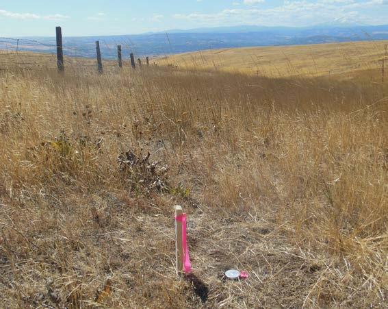
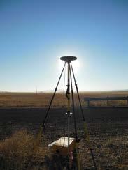
50 Left: Trimble R7 Receiver set up over GPS monument WASCO_40 Cover: Views of monument WASCO_25. Data collected for: Oregon Department of Geology and Mineral Industries 800 NE Oregon Street Suite 965 Portland, OR Prepared by: WSI, A Quantum Spatial Company 421 SW 6th Avenue Suite 800 Portland, Oregon phone: (503) fax: (503) SW 2nd Street Suite 400 Corvallis, OR phone: (541) fax: (541) ii

51 Contents 2 - Project Overview 3 - Aerial Acquisition 3 - LiDAR Survey 4 - Ground Survey 4 - Instrumentation 4 - Monumentation 6 - Methodology 7 - LiDAR Accuracy 7 - Relative Accuracy 8 - Vertical Accuracy 9 - Density 9 - Pulse Density 10 - Ground Density 12 - Appendix A : PLS Certification 13 - Appendix B : GPS Monument Table 1

52 Overview Project Overview WSI has completed the acquisition and processing of Light Detection and Ranging (LiDAR) data for the OLC Wasco County Delivery Area Four for the Oregon Department of Geology and Mineral Industries (DOGAMI). The Oregon LiDAR Consortium s Wasco County 2014 project area of interest (AOI) encompasses 1,020,680 acres. Delivery Area Four encompasses 67,682 acres. The collection of high resolution geographic data is part of an ongoing pursuit to amass a library of information accessible to government agencies as well as the general public. WSI LiDAR data acquisition for delivery areas one through four occurred from July 15 - September 19, Delivery area four was acquired from August 27-29, Settings for LiDAR data capture produced an average resolution of at least eight pulses per square meter. Final products created that are included in Delivery Area Four are LiDAR point cloud data, three-foot resolution digital elevation models of bare earth ground models and highest-hit returns, 1.5-foot intensity rasters, three-foot ground density rasters, study area vector shapes, ground survey points and monuments, and corresponding statistical data. WSI acquires and processes data in the most current, NGS-approved datums and geoid. For OLC Wasco County Delivery 4, all final deliverables are projected in Washington State Plane South, using the NAD83(2011) horizontal datum and the NAVD88 (Geoid 12A) vertical datum, with units in US Survey Feet. Study Area OLC Wasco County Delivery Four Data Delivered: April 24, 2015 Acquisition Dates 8/27/2014-8/29/2014 Delivery Area Four Area of Interest Projection Horizontal Datum Vertical Datum Units 67,682 acres Washington State Plane South NAD83 (2011) NAVD88 (Geoid 12A) US Survey Feet 2

53 Aerial Acquisition Aerial Acquisition LiDAR Survey The LiDAR survey used a Leica ALS70 and an Optech Orion H sensor mounted in a Cessna U206G, Partenavia P.68, and Piper Navajo. The systems were programmed to emit single pulses at a rate of 219 kilohertz and flown between 600 and 1,600 meters above ground level (AGL), capturing a scan angle of +/-15 degrees from nadir (field of view equal to 30 degrees). These settings are developed to yield points with an average native density of greater than eight pulses per square meter over terrestrial surfaces. Project Flightlines The native pulse density is the number of pulses emitted by the LiDAR system. Some types of surfaces such as dense vegetation or water may return fewer pulses than the laser originally emitted. Therefore, the delivered density can be less than the native density and lightly vary according to distributions of terrain, land cover, and water bodies. The study area was surveyed with opposing flight line side-lap of greater than 60 percent with at least 100 percent overlap to reduce laser shadowing and increase surface laser painting. The system allows up to four range measurements per pulse, and all discernible laser returns were processed for the output dataset. To solve for laser point position, it is vital to have an accurate description of aircraft position and attitude. Aircraft position is described as x, y, and z and measured twice per second (two hertz) by an onboard differential GPS unit. Aircraft attitude is measured 200 times per second (200 hertz) as pitch, roll, and yaw (heading) from an onboard inertial measurement unit (IMU). As illustrated in the accompanying map, 88 full and partial flightlines provide coverage of the delivery area four study area ,600 m AGL 30 OLC Wasco County LiDAR Acquisition Specifications Sensors Deployed Leica ALS 70 and Optech Orion H Aircraft Cessna U206G, Piper Navajo, Partenavia P.68 Survey Altitude (AGL) 600-1,600 meters Pulse Rate 219 khz Pulse Mode Single (SPiA) Field of View (FOV) 30 Roll Compensated Yes Overlap 100% overlap with 60% sidelap Pulse Emission Density 8 pulses per square meter 3

54 Ground Survey Ground Survey Ground control surveys, including monumentation, aerial targets, and ground survey points (GSPs) were conducted to support the airborne acquisition. Ground control data are used to geospatially correct the aircraft positional coordinate data and to perform quality assurance checks on final LiDAR data products. See the table to the right for specifications of equipment used. Instrumentation All Global Navigation Satellite System (GNSS) static surveys utilized Trimble R7 GNSS receivers with Zephyr Geodetic Model 2 RoHS antennas and Trimble R8 GNSS receivers with internal antennas. Rover surveys for GSP collection were conducted with Trimble R6, Trimble R8, and Trimble R10 GNSS receivers. Receiver Model Instrumentation Antenna OPUS Antenna ID Use Trimble R6 Integrated Antenna R6 TRMR6 Rover Trimble R7 Trimble R8 Zephyr GNSS Geodetic Model 2 RoHS Integrated Antenna R8 Model 2 TRM TRM_R8_GNSS Static Static, Rover Trimble R10 Integrated Antenna R10 TRMR10 Rover Monumentation Existing and newly established survey benchmarks serve as control points during LiDAR acquisition. Monument locations were selected with consideration for satellite visibility, field crew safety, and optimal location for GSP coverage. NGS benchmarks are preferred for control points; however, in the absence of NGS benchmarks, WSI produces our own monuments, and every effort is made to keep them within the public right of way or on public lands. If monuments are necessary on private property, consent from the owner is required. All monumentation is done with 5/8 x 30 rebar topped with a two-inch diameter aluminum cap stamped Watershed Sciences, Inc. Control. The table at right provides the list of monuments used in Delivery Area Four. See Appendix B for a complete list of monuments placed within the OLC Wasco County 2014 Study Area. Delivery Area Four GPS Monuments Ellipsoid PID Latitude Longitude Height (m) NAVD88 Height (m) RC WASCO_ WASCO_ Coordinates are on the NAD83 (2011) datum, epoch NAVD88 height referenced to Geoid12A. 4

55 Ground Survey 5

56 Ground Survey Methodology To correct the continuously recorded aircraft position, WSI concurrently conducts multiple static GNSS ground surveys over each monument. All control monuments are observed for a minimum of two survey sessions, each lasting no fewer than two hours. Data are collected at a rate of one hertz, using a 10 degree mask on the antenna. The static GPS data are then triangulated with nearby Continuously Operating Reference Stations (CORS) using the Online Positioning User Service (OPUS ) for precise positioning. Ground Survey Points (GSPs) are collected using Real Time Kinematic (RTK), Post-Processed Kinematic (PPK), and Fast- Static (FS) survey techniques. For RTK surveys, a base receiver is positioned at a nearby monument to broadcast a kinematic correction to a roving receiver; for PPK and FS surveys, however, these corrections are post-processed. All GSP measurements are made during periods with a Position Dilution of Precision (PDOP) no greater than 3.0 and in view of at least six satellites for both receivers. Relative errors for the position must be less than 1.5 centimeters horizontal and 2.0 centimeters vertical in order to be accepted. In order to facilitate comparisons with high quality LiDAR data, GSP measurements are not taken on highly reflective surfaces such as center line stripes or lane markings on roads. GSPs are taken no closer than one meter to any nearby terrain breaks such as road edges or drop offs. GSPs were collected within as many flight lines as possible; however, the distribution depended on ground access constraints and may not be equitably distributed throughout the study area. Monument Accuracy FGDC-STD Rating St Dev NE St Dev z 0.05 m Horiz 0.05 m Vert WSI ground professional collecting ground survey points in OLC Wasco County study area. Ground professional collecting RTK 6

57 Accuracy Results Accuracy Assessment In some cases statistics were generated for larger areas than the extent represented by delivered areas. Accuracy statistics are a product of calibration and data QA/QC methodology that are spatially coincident with production workflow, which at times exceeds the areal extent of delivery workflow. Relative Accuracy Relative accuracy refers to the internal consistency of the data set and is measured as the divergence between points from different flightlines within an overlapping area. Divergence is most apparent when flightlines are opposing. When the LiDAR system is well calibrated the line to line divergence is low (<10 centimeters). Internal consistency is affected by system attitude offsets (pitch, roll, and heading), mirror flex (scale), and GPS/IMU drift. Relative accuracy statistics are based on the comparison of 3,536 full and partial flightlines. Relative accuracy is reported for the cumulative delivered portions of the study area. Relative Accuracy Calibration Results N = 3,536 flightlines Project Average 0.13 ft. (0.04 m) Median Relative Accuracy 0.12 ft. (0.04 m) 1σ Relative Accuracy 0.13 ft. (0.04 m) Relative Accuracy Distribution Relative Accuracy Distribution 70% 60% 50% 40% 30% 20% 10% 3,536 Flightlines 0% Relative Accuracy (ft) Total Compared Points (n = 182,178,947,367) 2σ Relative Accuracy 0.22 ft. (0.07 m) 7

58 Accuracy Vertical Accuracy Vertical Accuracy reporting is designed to meet guidelines presented in the National Standard for Spatial Data Accuracy (NSSDA) (FGDC, 1998) and the ASPRS Guidelines for Vertical Accuracy Reporting for LiDAR Data V1.0 (ASPRS, 2004). The statistical model compares known ground survey points to the triangulated LiDAR surface. Vertical accuracy statistical analysis uses ground survey points in open areas where the LiDAR system has a very high probability that the sensor will measure the ground surface and is evaluated at the 95th percentile. For the OLC Wasco County 2014 Study area, 1,287 GSPs were used to calibrate Delivery Area Four. Vertical Accuracy is reported for the entire delivered study area and reported in the table below. For this project, no independent survey data were collected, nor were reserved points collected for testing. As such, vertical accuracy statistics are reported as Compiled to Meet. Sample Size (n) (ground survey points) Vertical Accuracy Results Delivery Area Four Cumulative 1,287 13,161 Root Mean Square Error 0.09 ft. (0.03 m) 0.10 ft. (0.03 m) 1 Standard Deviation 0.14 ft. (0.04 m) 0.13 ft. (0.04 m) 2 Standard Deviation 0.26 ft. (0.08 m) 0.25 ft. (0.08 m) Average Deviation 0.10 ft. (0.03 m) 0.09 ft. (0.03 m) Minimum Deviation ft. (-0.12 m) ft. (-0.14 m) Maximum Deviation 0.46ft. (0.14 m) 0.56 ft. (0.17 m) Vertical Accuracy Distribution GSP Absolute Error 60% 100% Absolute Error: Laser point to GCP Deviation 90% 0.60 RMSE 1 Sigma 2 Sigma Absolute Error Distribution 40% 20% 80% 70% 60% 50% 40% 30% 20% Cumulative Distribution Absolute Error Error (feet) % 0% 0% Deviation ~ Laser Point to Nearest Ground Survey Point (feet) Ground Survey Point Ground Survey Point 8

59 Density Density Pulse Density Final pulse density is calculated after processing and is a measure of first returns per sampled area. Some types of surfaces (e.g., dense vegetation, water) may return fewer pulses than the laser originally emitted. Therefore, the delivered density can be less than the native density and vary according to terrain, land cover, and water bodies. Density histograms and maps have been calculated based on first return laser pulse density and ground-classified laser point density. Densities are reported for the delivery area. Average Pulse Density pulses per square meter pulses per square foot Average Pulse Density per 0.75 USGS Quad. 30% 20% Percent Distribution 10% 0% Pulses per Square Foot 9

60 Density Ground Density Ground classifications were derived from ground surface modeling. Further classifications were performed by reseeding of the ground model where it was determined that the ground model failed, usually under dense vegetation and/or at breaks in terrain, steep slopes, and at tile boundaries. The classifications are influenced by terrain and grounding parameters that are adjusted for the dataset. The reported ground density is a measure of ground-classified point data for the delivery area. Ground Density points per square meter points per square foot Average ground density per 0.75 USGS Quad. 30% 20% Percent Distribution 10% 0% Ground Points per Square Foot 10

61 Appendix [ Page Intentionally Blank ] 11

62 Appendix A : PLS Certification Appendix 12

63 Appendix B : GPS Monument Table Appendix List of GPS monuments used in OLC Wasco County Survey Area. Coordinates are on the NAD83 (2011) datum, epoch NAVD88 height referenced to Geoid12A. OLC Wasco County GPS Monuments PID Latitude Longitude Ellipsoid Height (m) Orthometric Height (m) CISPUS_WSDOT RC RC WASCO_ WASCO_ WASCO_ WASCO_ WASCO_ WASCO_ WASCO_ WASCO_ WASCO_ WASCO_ WASCO_ WASCO_ WASCO_ WASCO_ WASCO_ WASCO_ WASCO_ WASCO_ WASCO_ WASCO_ WASCO_

64 Appendix OLC Wasco County GPS Monuments PID Latitude Longitude Ellipsoid Height (m) Orthometric Height (m) WASCO_ ' WASCO_ ' WASCO_ WASCO_ WASCO_ WASCO_ WASCO_ WASCO_ WASCO_ WASCO_ WASCO_ WASCO_ WASCO_ WASCO_ WASCO_ ' WASCO_ ' WASCO_ ' ' WASCO_ WASCO_ WASCO_ WASCO_ WASCO_ WASCO_ WASCO_ WASCO_

65 OLC Wasco County: Delivery Five July 1, 2015

66 Left: Trimble R7 Receiver set up over GPS monument WASCO_40 Cover: bare earth raster image created from LiDAR point of Butter Canyon. Data collected for: Oregon Department of Geology and Mineral Industries 800 NE Oregon Street Suite 965 Portland, OR Prepared by: WSI, A Quantum Spatial Company 421 SW 6th Avenue Suite 800 Portland, Oregon phone: (503) fax: (503) SW 2nd Street Suite 400 Corvallis, OR phone: (541) fax: (541) ii

67 Contents 2 - Project Overview 3 - Aerial Acquisition 3 - LiDAR Survey 4 - Ground Survey 4 - Instrumentation 4 - Monumentation 6 - Methodology 7 - LiDAR Accuracy 7 - Relative Accuracy 8 - Vertical Accuracy 9 - Density 9 - Pulse Density 10 - Ground Density 12 - Appendix A : PLS Certification 13 - Appendix B : GPS Monument Table 1

68 Overview Project Overview WSI has completed the acquisition and processing of Light Detection and Ranging (LiDAR) data for the OLC Wasco County Delivery Area Five for the Oregon Department of Geology and Mineral Industries (DOGAMI). The Oregon LiDAR Consortium s Wasco County 2014 project area of interest (AOI) encompasses 1,020,680 acres. Delivery Area Five encompasses 184,798 acres. The collection of high resolution geographic data is part of an ongoing pursuit to amass a library of information accessible to government agencies as well as the general public. WSI LiDAR data acquisition for delivery areas one through five occurred from July 15, February 11, Settings for LiDAR data capture produced an average resolution of at least eight pulses per square meter. Final products created that are included in Delivery Area Five are LiDAR point cloud data, three-foot resolution digital elevation models of bare earth ground models and highest-hit returns, 1.5-foot intensity rasters, three-foot ground density rasters, study area vector shapes, ground survey points and monuments, and corresponding statistical data. WSI acquires and processes data in the most current, NGS-approved datums and geoid. For OLC Wasco County delivery area five, all final deliverables are projected in Oregon Statewide Lambert (OGIC), using the NAD83(2011) horizontal datum and the NAVD88 (Geoid 12A) vertical datum, with units in International Feet. Study Area OLC Wasco County Delivery Five Data Delivered: April 24, 2015 Acquisition Dates 7/30/2014-2/11/2015 Delivery Area Five 184,798 acres Area of Interest Projection OREGON STATEWIDE LAMBERT (OGIC) Horizontal datum NAD83 (2011) Epoch Vertical datum NAVD88 (Geoid 12A) Units International Feet 2

69 Aerial Acquisition Aerial Acquisition LiDAR Survey The LiDAR survey used a Leica ALS70 and an Optech Orion H sensor mounted in a Cessna U206G, Partenavia P.68, and Piper Navajo. The systems were programmed to emit single pulses at a rate of 219 kilohertz and flown between 600 and 1,600 meters above ground level (AGL), capturing a scan angle of +/-15 degrees from nadir (field of view equal to 30 degrees). These settings are developed to yield points with an average native density of greater than eight pulses per square meter over terrestrial surfaces. Project Flightlines The native pulse density is the number of pulses emitted by the LiDAR system. Some types of surfaces such as dense vegetation or water may return fewer pulses than the laser originally emitted. Therefore, the delivered density can be less than the native density and lightly vary according to distributions of terrain, land cover, and water bodies. The study area was surveyed with opposing flight line side-lap of greater than 60 percent with at least 100 percent overlap to reduce laser shadowing and increase surface laser painting. The system allows up to four range measurements per pulse, and all discernible laser returns were processed for the output dataset. To solve for laser point position, it is vital to have an accurate description of aircraft position and attitude. Aircraft position is described as x, y, and z and measured twice per second (two hertz) by an onboard differential GPS unit. Aircraft attitude is measured 200 times per second (200 hertz) as pitch, roll, and yaw (heading) from an onboard inertial measurement unit (IMU). As illustrated in the accompanying map, 653 full and partial flightlines provide coverage of the delivery area five study area ,600 m AGL 30 OLC Wasco County LiDAR Acquisition Specifications Sensors Deployed Leica ALS 70 and Optech Orion H Aircraft Cessna U206G, Piper Navajo, Partenavia P.68 Survey Altitude (AGL) 600-1,600 meters Pulse Rate 219 khz Pulse Mode Single (SPiA) Field of View (FOV) 30 Roll Compensated Yes Overlap 100% overlap with 60% sidelap Pulse Emission Density 8 pulses per square meter 3

70 Ground Survey Ground Survey Ground control surveys, including monumentation, aerial targets, and ground survey points (GSPs) were conducted to support the airborne acquisition. Ground control data are used to geospatially correct the aircraft positional coordinate data and to perform quality assurance checks on final LiDAR data products. See the table to the right for specifications of equipment used. Instrumentation All Global Navigation Satellite System (GNSS) static surveys utilized Trimble R7 GNSS receivers with Zephyr Geodetic Model 2 RoHS antennas and Trimble R8 GNSS receivers with internal antennas. Rover surveys for GSP collection were conducted with Trimble R6, Trimble R8, and Trimble R10 GNSS receivers. Monumentation Existing and newly established survey benchmarks serve as control points during LiDAR acquisition. Monument locations were selected with consideration for satellite visibility, field crew safety, and optimal location for GSP coverage. NGS benchmarks are preferred for control points; however, in the absence of NGS benchmarks, WSI produces our own monuments, and every effort is made to keep them within the public right of way or on public lands. If monuments are necessary on private property, consent from the owner is required. All monumentation is done with 5/8 x 30 rebar topped with a two-inch diameter aluminum cap stamped Watershed Sciences, Inc. Control. The table at right provides the list of monuments used in Delivery Area Five. See Appendix B for a complete list of monuments placed within the OLC Wasco County 2014 Study Area. Receiver Model Instrumentation Antenna OPUS Antenna ID Use Trimble R6 Integrated Antenna R6 TRMR6 Rover Trimble R7 Trimble R8 Zephyr GNSS Geodetic Model 2 RoHS Integrated Antenna R8 Model 2 TRM TRM_R8_GNSS Delivery Area Five GPS Monuments Ellipsoid PID Latitude Longitude Height (m) Static Static, Rover Trimble R10 Integrated Antenna R10 TRMR10 Rover NAVD88 Height (m) RC WASCO_ WASCO_ WASCO_ WASCO_ WASCO_ WASCO_ WASCO_ Coordinates are on the NAD83 (2011) datum, epoch NAVD88 height referenced to Geoid12A. Trimble R7 set up over GPS monument Wasco_16. 4

71 Ground Survey WASCO_13 WASCO_16 WASCO_18 WASCO_34 WASCO_17 WASCO_28 WASCO_27 RC1228 5

72 Ground Survey Methodology To correct the continuously recorded aircraft position, WSI concurrently conducts multiple static GNSS ground surveys over each monument. All control monuments are observed for a minimum of two survey sessions, each lasting no fewer than two hours. Data are collected at a rate of one hertz, using a 10 degree mask on the antenna. The static GPS data are then triangulated with nearby Continuously Operating Reference Stations (CORS) using the Online Positioning User Service (OPUS) for precise positioning. Ground Survey Points (GSPs) are collected using Real Time Kinematic (RTK), Post-Processed Kinematic (PPK), and Fast-Static (FS) survey techniques. For RTK surveys, a base receiver is positioned at a nearby monument to broadcast a kinematic correction to a roving receiver; for PPK and FS surveys, however, these corrections are post-processed. All GSP measurements are made during periods with a Position Dilution of Precision (PDOP) no greater than 3.0 and in view of at least six satellites for both receivers. Relative errors for the position must be less than 1.5 centimeters horizontal and 2.0 centimeters vertical in order to be accepted. In order to facilitate comparisons with high quality LiDAR data, GSP measurements are not taken on highly reflective surfaces such as center line stripes or lane markings on roads. GSPs are taken no closer than one meter to any nearby terrain breaks such as road edges or drop offs. GSPs were collected within as many flight lines as possible; however, the distribution depended on ground access constraints and may not be equitably distributed throughout the study area. Monument Accuracy FGDC-STD Rating St Dev NE St Dev z 0.05 m Horiz 0.05 m Vert WSI ground professional collecting ground survey points in OLC Wasco County study area. Ground professional collecting RTK 6

73 Accuracy Results Accuracy Assessment In some cases statistics were generated for larger areas than the extent represented by delivered areas. Accuracy statistics are a product of calibration and data QA/QC methodology that are spatially coincident with production workflow, which at times exceeds the areal extent of delivery workflow. Relative Accuracy Relative accuracy refers to the internal consistency of the data set and is measured as the divergence between points from different flightlines within an overlapping area. Divergence is most apparent when flightlines are opposing. When the LiDAR system is well calibrated the line to line divergence is low (<10 centimeters). Internal consistency is affected by system attitude offsets (pitch, roll, and heading), mirror flex (scale), and GPS/IMU drift. Relative accuracy statistics are based on the comparison of 3,536 full and partial flightlines. Relative accuracy is reported for the cumulative delivered portions of the study area. Relative Accuracy Calibration Results N = 3,536 flightlines Project Average 0.13 ft. (0.04 m) Median Relative Accuracy 0.12 ft. (0.04 m) 1σ Relative Accuracy 0.13 ft. (0.04 m) Relative Accuracy Distribution Relative Accuracy Distribution 70% 60% 50% 40% 30% 20% 10% 3,536 Flightlines 0% Relative Accuracy (ft) Total Compared Points (n = 182,178,947,367) 2σ Relative Accuracy 0.22 ft. (0.07 m) 7

74 Accuracy Vertical Accuracy Vertical Accuracy reporting is designed to meet guidelines presented in the National Standard for Spatial Data Accuracy (NSSDA) (FGDC, 1998) and the ASPRS Guidelines for Vertical Accuracy Reporting for LiDAR Data V1.0 (ASPRS, 2004). The statistical model compares known ground survey points to the triangulated LiDAR surface. Vertical accuracy statistical analysis uses ground survey points in open areas where the LiDAR system has a very high probability that the sensor will measure the ground surface and is evaluated at the 95th percentile. For the OLC Wasco County 2014 Study area, 1,287 GSPs were used to calibrate Delivery Area Five. Vertical Accuracy is reported for the entire delivered study area and reported in the table below. For this project, no independent survey data were collected, nor were reserved points collected for testing. As such, vertical accuracy statistics are reported as Compiled to Meet. Vertical Accuracy Results Sample Size (n) (ground survey points) Cumulative 13,161 Root Mean Square Error 0.10 ft. (0.03 m) 1 Standard Deviation 0.13 ft. (0.04 m) 2 Standard Deviation 0.25 ft. (0.08 m) Average Deviation 0.09 ft. (0.03 m) Minimum Deviation ft. (-0.14 m) Maximum Deviation 0.56 ft. (0.17 m) Vertical Accuracy Distribution GSP Absolute Error 60% 100% Absolute Error: Laser point to GCP Deviation 90% 0.60 RMSE 1 Sigma 2 Sigma Absolute Error Distribution 40% 20% 80% 70% 60% 50% 40% 30% 20% Cumulative Distribution Absolute Error Error (feet) % 0% 0% Deviation ~ Laser Point to Nearest Ground Survey Point (feet) Ground Survey Point Ground Survey Point 8

75 Density Density Pulse Density Final pulse density is calculated after processing and is a measure of first returns per sampled area. Some types of surfaces (e.g., dense vegetation, water) may return fewer pulses than the laser originally emitted. Therefore, the delivered density can be less than the native density and vary according to terrain, land cover, and water bodies. Density histograms and maps have been calculated based on first return laser pulse density and ground-classified laser point density. Densities are reported for the delivery area. Average Pulse Density Average Pulse Density per 0.75 USGS Quad. pulses per square meter pulses per square foot % 30% Percent Distribution 20% 10% 0% Pulses per Square Foot 9

76 Density Ground Density Ground classifications were derived from ground surface modeling. Further classifications were performed by reseeding of the ground model where it was determined that the ground model failed, usually under dense vegetation and/or at breaks in terrain, steep slopes, and at tile boundaries. The classifications are influenced by terrain and grounding parameters that are adjusted for the dataset. The reported ground density is a measure of ground-classified point data for the delivery area. Ground Density points per square meter points per square foot Average ground density per 0.75 USGS Quad. 50% 40% Percent Distribution 30% 20% 10% 0% Ground Points per Square Foot 10

77 Appendix [ Page Intentionally Blank ] 11

78 Appendix A : PLS Certification Appendix 6/17/

79 Appendix B : GPS Monument Table Appendix List of GPS monuments used in OLC Wasco County Survey Area. Coordinates are on the NAD83 (2011) datum, epoch NAVD88 height referenced to Geoid12A. OLC Wasco County GPS Monuments PID Latitude Longitude Ellipsoid Height (m) Orthometric Height (m) CISPUS_WSDOT RC RC WASCO_ WASCO_ WASCO_ WASCO_ WASCO_ WASCO_ WASCO_ WASCO_ WASCO_ WASCO_ WASCO_ WASCO_ WASCO_ WASCO_ WASCO_ WASCO_ WASCO_ WASCO_ WASCO_ WASCO_ WASCO_ WASCO_ ' WASCO_ '

80 Appendix OLC Wasco County GPS Monuments PID Latitude Longitude Ellipsoid Height (m) Orthometric Height (m) WASCO_ WASCO_ WASCO_ WASCO_ WASCO_ WASCO_ WASCO_ WASCO_ WASCO_ WASCO_ WASCO_ WASCO_ WASCO_ ' WASCO_ ' WASCO_ ' ' WASCO_ WASCO_ WASCO_ WASCO_ WASCO_ WASCO_ WASCO_ WASCO_ WASCO_ WASCO_ WASCO_ WASCO_

81 OLC Wasco County: Delivery Six December 22, 2015

82 Left: Trimble R7 Receiver set up over GPS monument WASCO_40 Cover: bare earth raster image created from LiDAR point of Butter Canyon. Data collected for: Oregon Department of Geology and Mineral Industries 800 NE Oregon Street Suite 965 Portland, OR Prepared by: WSI, A Quantum Spatial Company 421 SW 6th Avenue Suite 800 Portland, Oregon phone: (503) fax: (503) SW 2nd Street Suite 400 Corvallis, OR phone: (541) fax: (541) ii

83 Contents 2 - Project Overview 3 - Aerial Acquisition 3 - LiDAR Survey 4 - Ground Survey 4 - Instrumentation 4 - Monumentation 6 - Methodology 7 - LiDAR Accuracy 7 - Relative Accuracy 8 - Vertical Accuracy 9 - Density 9 - Pulse Density 10 - Ground Density 12 - Appendix A : PLS Certification 13 - Appendix B : GPS Monument Table 1

84 Overview Project Overview WSI has completed the acquisition and processing of Light Detection and Ranging (LiDAR) data for the OLC Wasco County Delivery Area Six for the Oregon Department of Geology and Mineral Industries (DOGAMI). The Oregon LiDAR Consortium s Wasco County project area of interest (AOI) encompasses 1,020,680 acres. Delivery Area Six encompasses 317,371 acres. The collection of high resolution geographic data is part of an ongoing pursuit to amass a library of information accessible to government agencies as well as the general public. LiDAR data acquisition for delivery areas one through six occurred from July 15, August 5, Settings for LiDAR data capture produced an average resolution of at least eight pulses per square meter. Final products created that are included in Delivery Area Five are LiDAR point cloud data, three-foot resolution digital elevation models of bare earth ground models and highest-hit returns, 1.5-foot intensity rasters, three-foot ground density rasters, study area vector shapes, ground survey points and monuments, and corresponding statistical data. WSI acquires and processes data in the most current, NGS-approved datums and geoid. For OLC Wasco County delivery area six, all final deliverables are projected in Washington State Plane South, using the NAD83(2011) horizontal datum and the NAVD88 (Geoid 12A) vertical datum, with units in US Survey Feet. Study Area OLC Wasco County Delivery Six Data Delivered: December 18, 2015 Acquisition Dates 8/27/2014-8/5/2015 Delivery Area Six Data Extent Projection Horizontal datum 317,371 acres Washington State Plane South NAD83 (2011) Epoch Vertical datum NAVD88 (Geoid 12A) Units US Survey Feet 2

85 Aerial Acquisition Aerial Acquisition LiDAR Survey The LiDAR survey used a Leica ALS70 sensor mounted in a Cessna Grand Caravan. The system was programmed to emit single pulses at a rate of 198 kilohertz and flown around 1,400 meters above ground level (AGL), capturing a scan angle of +/-15 degrees from nadir (field of view equal to 30 degrees). These settings are developed to yield points with an average native density of greater than eight pulses per square meter over terrestrial surfaces. Project Flightlines The native pulse density is the number of pulses emitted by the LiDAR system. Some types of surfaces such as dense vegetation or water may return fewer pulses than the laser originally emitted. Therefore, the delivered density can be less than the native density and lightly vary according to distributions of terrain, land cover, and water bodies. The study area was surveyed with opposing flight line side-lap of greater than 60 percent with at least 100 percent overlap to reduce laser shadowing and increase surface laser painting. The system allows up to four range measurements per pulse, and all discernible laser returns were processed for the output dataset. To solve for laser point position, it is vital to have an accurate description of aircraft position and attitude. Aircraft position is described as x, y, and z and measured twice per second (two hertz) by an onboard differential GPS unit. Aircraft attitude is measured 200 times per second (200 hertz) as pitch, roll, and yaw (heading) from an onboard inertial measurement unit (IMU). As illustrated in the accompanying map, 809 full and partial flightlines provide coverage of the delivery area six study area. 1,400 m AGL 30 OLC Wasco County LiDAR Acquisition Specifications Sensors Deployed Leica ALS 70 Aircraft Cessna Grand Caravan Survey Altitude (AGL) 1,400 meters Pulse Rate 198 khz Pulse Mode Single (SPiA) Field of View (FOV) 30 Roll Compensated Yes Overlap 100% overlap with 60% sidelap Pulse Emission Density 8 pulses per square meter 3

86 Ground Survey Ground Survey Ground control surveys, including monumentation, aerial targets, and ground survey points (GSPs) were conducted to support the airborne acquisition. Ground control data are used to geospatially correct the aircraft positional coordinate data and to perform quality assurance checks on final LiDAR data products. See the table to the right for specifications of equipment used. Receiver Model Instrumentation Antenna OPUS Antenna ID Use Trimble R6 Integrated Antenna R6 TRMR6 Rover Instrumentation Trimble R7 Zephyr GNSS Geodetic Model 2 RoHS TRM Static All Global Navigation Satellite System (GNSS) static surveys utilized Trimble R7 GNSS receivers with Zephyr Geodetic Model 2 RoHS antennas and Trimble R8 GNSS receivers with internal antennas. Rover surveys for GSP collection were conducted with Trimble R6, Trimble R8, and Trimble R10 GNSS receivers. Monumentation Ground control surveys, including monumentation, and ground survey points (GSPs), were conducted to support the airborne acquisition. Ground control data were used to geospatially correct the aircraft positional coordinate data and to perform quality assurance checks on final LiDAR data. The spatial configuration of ground survey monuments provided redundant control within 13 nautical miles of the mission areas for LiDAR flights. Monuments were also used for collection of ground survey points using real time kinematic (RTK). Monument locations were selected with consideration for satellite visibility, field crew safety, and optimal location for GSP coverage. QSI established two new monuments for the PGE Tucannon Wind Farm LiDAR project (Table on Page 6). New monumentation was set using 5/8 x 30 rebar topped with stamped 2-1/2 aluminum caps. QSI s professional land surveyor, Christopher Glantz (WA PLS #48755) oversaw and certified the establishment of all monuments. To correct the continuously recorded onboard measurements of the aircraft position, QSI concurrently conducted multiple static Global Navigation Satellite System (GNSS) ground surveys (1 Hz recording frequency) over each monument. During post-processing, the static GPS data were triangulated with nearby Continuously Operating Reference Stations (CORS) using the Online Positioning User Service (OPUS) for precise positioning. Multiple independent sessions over the same monument were processed to confirm antenna height measurements and to refine position accuracy. The table at right provides the list of monuments used in Delivery Area Six. See Appendix B for a complete list of monuments placed within the OLC Wasco County Study Area. Trimble R8 Integrated Antenna R8 Model 2 TRM_R8_GNSS Static, Rover Trimble R10 Integrated Antenna R10 TRMR10 Rover PID Latitude Longitude CISPUS_ WSDOT Ellipsoid Height (m) NAVD88 Height (m) RC RC WASCO_ WASCO_ WASCO_ WASCO_ WASCO_ WASCO_ WASCO_ WASCO_ WASCO_ WASCO_ WASCO_ WASCO_ WASCO_ WASCO_ WASCO_ WASCO_ WASCO_ WASCO_ WASCO_ WASCO_ Coordinates are on the NAD83 (2011) datum, epoch NAVD88 height referenced to Geoid12A. 4

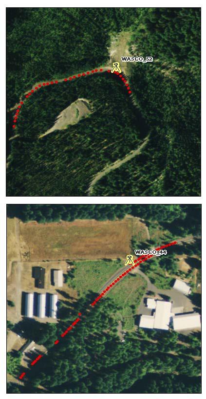
87 Ground Survey 5

88 Ground Survey Methodology Ground survey points (GSPs) are collected using Real Time Kinematic (RTK) and Post Processed Kinematic (PPK) survey techniques. For RTK surveys, a Trimble R7 base unit was set up over an appropriate monument to broadcast a real-time correction to a roving R6 unit. This RTK rover survey allows for precise location measurement (2.0 centimeter). All RTK measurements were made during periods with a Position Dilution of Precision (PDOP) of less than 3.0 and in view of at least six satellites by the stationary reference and roving receiver. For RTK data, the collector recorded at least a five-second stationary observation, and then calculated the pseudorange position from three one-second epochs with relative error less than 1.5 centimeter horizontal and 2.0 centimeter vertical. GSP positions were collected on bare earth locations such as paved, gravel or stable dirt roads, and other locations where the ground was clearly visible (and was likely to remain visible) from the sky during the data acquisition and GSP measurement periods. In order to facilitate comparisons with LiDAR data, GSP measurements were not taken on highly reflective surfaces such as center line stripes or lane markings on roads. The planned locations for control points were determined prior to field deployment, and the suitability of these locations was verified on site. The distribution of ground survey points depended on ground access constraints, and may not be equitably distributed throughout the study area. Monument Accuracy FGDC-STD Rating St Dev NE St Dev z 0.05 m Horiz 0.05 m Vert WSI ground professional collecting ground survey points in OLC Wasco County study area. Ground professional collecting RTK 6

89 Accuracy Results Accuracy Assessment In some cases statistics were generated for larger areas than the extent represented by delivered areas. Accuracy statistics are a product of calibration and data QA/QC methodology that are spatially coincident with production workflow, which at times exceeds the areal extent of delivery workflow. Relative Accuracy Relative accuracy refers to the internal consistency of the data set and is measured as the divergence between points from different flightlines within an overlapping area. Divergence is most apparent when flightlines are opposing. When the LiDAR system is well calibrated the line to line divergence is low (<10 centimeters). Internal consistency is affected by system attitude offsets (pitch, roll, and heading), mirror flex (scale), and GPS/IMU drift. Relative accuracy statistics are based on the comparison of 4,343 full and partial flightlines. Relative accuracy is reported for the cumulative delivered portions of the study area. Relative Accuracy Calibration Results N = 4,343 flightlines Project Average ft. (0.045 m) Median Relative Accuracy ft. (0.039 m) 1σ Relative Accuracy ft. (0.045 m) Relative Accuracy Distribution Relative Accuracy Distribution 60% 50% 40% 30% 20% 10% 4,343 Flightlines 0% Relative Accuracy (ft) Total Compared Points (n = 200,281,287,596) 2σ Relative Accuracy ft. (0.079 m) 7

90 Accuracy Vertical Accuracy Vertical Accuracy reporting is designed to meet guidelines presented in the National Standard for Spatial Data Accuracy (NSSDA) (FGDC, 1998) and the ASPRS Guidelines for Vertical Accuracy Reporting for LiDAR Data V1.0 (ASPRS, 2004). The statistical model compares known ground survey points to the triangulated LiDAR surface. Vertical accuracy statistical analysis uses ground survey points in open areas where the LiDAR system has a very high probability that the sensor will measure the ground surface and is evaluated at the 95th percentile. For the OLC Wasco County Study area, 2,269 GSPs were used to calibrate Delivery Area Six. Vertical Accuracy is reported for the entire delivered study area and reported in the table below. For this project, no independent survey data were collected, nor were reserved points collected for testing. As such, vertical accuracy statistics are reported as Compiled to Meet. Sample Size (n) (ground survey points) Vertical Accuracy Results Delivery 6 Cumulative 2,269 15,430 Root Mean Square Error ft. (0.035 m) ft. (0.030 m) 1 Standard Deviation ft. (0.042 m) ft. (0.041 m) 2 Standard Deviation ft. (0.082 m) ft. (0.077 m) Average Deviation ft. (0.034 m) ft. (0.033 m) Minimum Deviation ft. ( m) ft. ( m) Maximum Deviation ft. (0.142 m) ft. (0.171 m) Cumulative Vertical Accuracy Distribution Cumulative GSP Absolute Error 60% 100% Absolute Error: Laser point to GCP Deviation 90% 80% 0.60 RMSE 1 Sigma 2 Sigma Absolute Error Distribution 40% 20% 0% 70% 60% 50% 40% 30% 20% 10% 0% Deviation ~ Laser Point to Nearest Ground Survey Point (feet) Cumulative Distribution Absolute Error (feet) Absolute Error (feet) Ground Survey Point 8

91 Density Pulse Density Density Final pulse density is calculated after processing and is a measure of first returns per sampled area. Some types of surfaces (e.g., dense vegetation, water) may return fewer pulses than the laser originally emitted. Therefore, the delivered density can be less than the native density and vary according to terrain, land cover, and water bodies. Density histograms and maps have been calculated based on first return laser pulse density and ground-classified laser point density. Densities are reported for the delivery area. Average Pulse Density per 0.75 USGS Quad. Delivery 6 Pulse Density Cumulative Pulse Density pulses per square meter pulses per square foot pulses per square meter pulses per square foot % Percent Distribution 20% 10% 0% Pulses per Square Foot 9

92 Density Ground Density Ground classifications were derived from ground surface modeling. Further classifications were performed by reseeding of the ground model where it was determined that the ground model failed, usually under dense vegetation and/or at breaks in terrain, steep slopes, and at tile boundaries. The classifications are influenced by terrain and grounding parameters that are adjusted for the dataset. The reported ground density is a measure Average ground density per 0.75 USGS Quad. Delivery 6 Ground Density points per square meter points per square foot Cumulative Ground Density points per square meter points per square foot % 40% Percent Distribution 30% 20% 10% 0% Ground Points per Square Foot 10

93 Appendix [ Page Intentionally Blank ] 11

94 Appendix A : PLS Certification Appendix 12/21/

95 Appendix B : GPS Monument Table Appendix List of GPS monuments used in OLC Wasco County Survey Area. Coordinates are on the NAD83 (2011) datum, epoch NAVD88 height referenced to Geoid12A. OLC Wasco County GPS Monuments PID Latitude Longitude Ellipsoid Height (m) Orthometric Height (m) CISPUS_WSDOT RC RC WASCO_ WASCO_ WASCO_ WASCO_ WASCO_ WASCO_ WASCO_ WASCO_ WASCO_ WASCO_ WASCO_ WASCO_ WASCO_ WASCO_ WASCO_ WASCO_ WASCO_ WASCO_ WASCO_ WASCO_ WASCO_ WASCO_ ' WASCO_ '