Final Exam. CSE 2011 Prof. J. Elder Last Updated: :41 PM

Transcription

1 Final Exam Ø Tue, 17 Apr :00 22:00 LAS B Ø Closed Book Ø Format similar to midterm Ø Will cover whole course, with emphasis on material after midterm (maps, hashing, binary search trees, sorting, graphs) - 1 -

2 Suggested Study Strategy Ø Review and understand the slides. Ø Read the textbook, especially where concepts and methods are not yet clear to you. Ø Do all of the practice problems I provide (available early next week). Ø Do extra practice problems from the textbook. Ø Review the midterm and solutions for practice writing this kind of exam. Ø Practice writing clear, succint pseudocode! Ø See me or one of the TAs if there is anything that is still not clear

3 Assistance Ø Regular office hours will not be held Ø You may see Ron, Paria or me by appointment - 3 -

4 End of Term Review - 4 -

5 Summary of Topics 1. Maps 2. Binary Search Trees 3. Sorting 4. Graphs - 5 -

6 Maps Ø A map models a searchable collection of key-value entries Ø The main operations of a map are for searching, inserting, and deleting items Ø Multiple entries with the same key are not allowed Ø Applications: q address book q student-record database - 6 -

7 Ø Map ADT methods: The Map ADT q get(k): if the map M has an entry with key k, return its associated value; else, return null q put(k, v): insert entry (k, v) into the map M; if key k is not already in M, then return null; else, return old value associated with k q remove(k): if the map M has an entry with key k, remove it from M and return its associated value; else, return null q size(), isempty() q keys(): return an iterator of the keys in M q values(): return an iterator of the values in M q entries(): returns an iterator of the entries in M - 7 -

8 Performance of a List-Based Map Ø Performance: q put, get and remove take O(n) time since in the worst case (the item is not found) we traverse the entire sequence to look for an item with the given key Ø The unsorted list implementation is effective only for small maps - 8 -

9 Hash Tables Ø A hash table is a data structure that can be used to make map operations faster. Ø While worst-case is still O(n), average case is typically O(1)

10 Hash Functions and Hash Tables Ø A hash function h maps keys of a given type to integers in a fixed interval [0, N - 1] Ø Example: h(x) = x mod N is a hash function for integer keys Ø The integer h(x) is called the hash value of key x Ø A hash table for a given key type consists of q Hash function h q Array (called table) of size N Ø When implementing a map with a hash table, the goal is to store item (k, o) at index i = h(k)

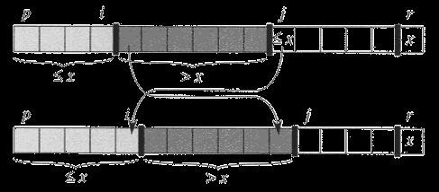
11 Ø Polynomial accumulation: Polynomial Hash Codes q We partition the bits of the key into a sequence of components of fixed length (e.g., 8, 16 or 32 bits) a 0 a 1 a n-1 q We evaluate the polynomial p(z) = a 0 + a 1 z + a 2 z2 + + a n-1 z n-1 at a fixed value z, ignoring overflows q Especially suitable for strings (e.g., the choice z = 33 gives at most 6 collisions on a set of 50,000 English words) q Polynomial p(z) can be evaluated in O(n) time using Horner s rule: ² The following polynomials are successively computed, each from the previous one in O(1) time p 0 (z) = a n-1 q We have p(z) = p n-1 (z) p i (z) = a n-i-1 + zp i-1 (z) (i = 1, 2,, n -1)

12 Compression Functions Ø Division: q h 2 (y) = y mod N q The size N of the hash table is usually chosen to be a prime Ø Multiply, Add and Divide (MAD): q h 2 (y) = (ay + b) mod N q a and b are nonnegative integers such that a mod N 0 q Otherwise, every integer would map to the same value b

13 Collision Handling Ø Collisions occur when different elements are mapped to the same cell Ø Separate Chaining: q Let each cell in the table point to a linked list of entries that map there q Separate chaining is simple, but requires additional memory outside the table 0 Ø Ø Ø

14 Linear Probing Ø Open addressing: the colliding item is placed in a different cell of the table Ø Linear probing handles collisions by placing the colliding item in the next (circularly) available table cell Ø Each table cell inspected is referred to as a probe Ø Colliding items lump together, so that future collisions cause a longer sequence of probes Ø Example: q h(x) = x mod 13 q Insert keys 18, 41, 22, 44, 59, 32, 31, 73, in this order

15 Performance of Hashing Ø In the worst case, searches, insertions and removals on a hash table take O(n) time Ø The worst case occurs when all the keys inserted into the map collide Ø The load factor λ = n/n affects the performance of a hash table q For separate chaining, performance is typically good for λ < 0.9. q For open addressing, performance is typically good for λ < 0.5. q java.util.hashmap maintains λ < 0.75 Ø Separate chaining is typically as fast or faster than open addressing

16 DICTIONARIES

17 Dictionary ADT Ø The dictionary ADT models a searchable collection of keyelement entries Ø The main operations of a dictionary are searching, inserting, and deleting items Ø Multiple items with the same key are allowed Ø Applications: q word-definition pairs q credit card authorizations q DNS mapping of host names (e.g., datastructures.net) to internet IP addresses (e.g., ) Ø Dictionary ADT methods: q get(k): if the dictionary has at least one entry with key k, returns one of them, else, returns null q getall(k): returns an iterable collection of all entries with key k q put(k, v): inserts and returns the entry (k, v) q remove(e): removes and returns the entry e. Throws an exception if the entry is not in the dictionary. q entryset(): returns an iterable collection of the entries in the dictionary q size(), isempty()

18 Dictionaries & Ordered Search Tables Ø If keys obey a total order relation, can represent dictionary as an ordered search table stored in an array. Ø Can then support a fast find(k) using binary search. q at each step, the number of candidate items is halved q terminates after a logarithmic number of steps q Example: find(7) 0 l 0 l m h m h l m h l=m =h

19 BinarySearch(A[1..n], key) <precondition>: A[1..n] is sorted in non-decreasing order <postcondition>: If key is in A[1..n], algorithm returns its location p = 1, q = n while q > p < loop-invariant>: If key is in A[1..n], then key is in A[p.. q] p + q mid = 2 if key A[ mid ] q = mid else p = mid + 1 end end if key = A[ p] return( p) else return("key not in list") end

20 Topic 1. Binary Search Trees

21 Binary Search Trees Ø Insertion Ø Deletion Ø AVL Trees Ø Splay Trees

22 Binary Search Trees Ø A binary search tree is a binary tree storing key-value entries at its internal nodes and satisfying the following property: q Let u, v, and w be three nodes such that u is in the left subtree of v and w is in the right subtree of v. We have key(u) key(v) key(w) Ø The textbook assumes that external nodes are placeholders : they do not store entries (makes algorithms a little simpler) Ø An inorder traversal of a binary search trees visits the keys in increasing order Ø Binary search trees are ideal for maps or dictionaries with ordered keys

23 Binary Search Tree All nodes in left subtree Any node All nodes in right subtree

24 Ø Cut sub-tree in half. Search: Define Step Ø Determine which half the key would be in. Ø Keep that half. key If key < root, then key is in left half. If key = root, then key is found If key > root, then key is in right half

25 Insertion (For Dictionary) Ø To perform operation insert(k, o), we search for key k (using TreeSearch) Ø Suppose k is not already in the tree, and let w be the leaf reached by the search Ø We insert k at node w and expand w into an internal node Ø Example: insert 5 w < > > w

26 Insertion Ø Suppose k is already in the tree, at node v. Ø We continue the downward search through v, and let w be the leaf reached by the search Ø Note that it would be correct to go either left or right at v. We go left by convention. Ø We insert k at node w and expand w into an internal node Ø Example: insert 6 2 < > > w w

27 Deletion Ø To perform operation remove(k), we search for key k Ø Suppose key k is in the tree, and let v be the node storing k Ø If node v has a leaf child w, we remove v and w from the tree with operation removeexternal(w), which removes w and its parent Ø Example: remove 4 < > 1 4 v 8 w

28 Deletion (cont.) Ø Now consider the case where the key k to be removed is stored at a node v whose children are both internal q we find the internal node w that follows v in an inorder traversal q we copy the entry stored at w into node v q we remove node w and its left child z (which must be a leaf) by means of operation removeexternal(z) Ø Example: remove v 1 5 v w z

29 Performance Ø Consider a dictionary with n items implemented by means of a binary search tree of height h q the space used is O(n) q methods find, insert and remove take O(h) time Ø The height h is O(n) in the worst case and O(log n) in the best case Ø It is thus worthwhile to balance the tree (next topic)!

30 AVL Trees Ø AVL trees are balanced. Ø An AVL Tree is a binary search tree in which the heights of siblings can differ by at most height

31 Height of an AVL Tree Ø Claim: The height of an AVL tree storing n keys is O(log n)

32 Insertion Ø Imbalance may occur at any ancestor of the inserted node. height = 3 7 height = Insert(2) 3 4 Problem!

33 Ø Step 1: Search Insertion: Rebalancing Strategy q Starting at the inserted node, traverse toward the root until an imbalance is discovered. height = Problem!

34 Insertion: Rebalancing Strategy Ø Step 2: Repair q The repair strategy is called trinode restructuring. q 3 nodes x, y and z are distinguished: ² z = the parent of the high sibling ² y = the high sibling ² x = the high child of the high sibling q We can now think of the subtree 3 rooted at z as consisting of these 3 nodes plus their 4 subtrees height = Problem!

35 Insertion: Trinode Restructuring Example Note that y is the middle value. height = h z h-1 y Restructure h-1 y h-3 T 3 h-2 x h-2 z h-2 x h-3 T 2 h-3 h-3 T 0 T 1 T 2 T 3 T 0 T 1 one is h-3 & one is h-4 one is h-3 & one is h

36 Insertion: Trinode Restructuring - 4 Cases Ø There are 4 different possible relationships between the three nodes x, y and z before restructuring: x y z z y x y x z z x y height = h z height = h z height = h z height = h z y h-1 h-3 T 3 y h-3 h-1 T 0 y h-1 h-3 T 3 y h-3 h-1 T 0 h-2 x h-3 h-3 x h-2 h-3 h-2 x x h-2 h-3 T 2 T 1 T 0 T 3 T 0 T 1 T 2 T 3 T 1 T 2 T 1 T 2 one is h-3 & one is h-4 one is h-3 & one is h-4 one is h-3 & one is h-4 one is h-3 & one is h

37 Insertion: Trinode Restructuring - The Whole Tree Ø Do we have to repeat this process further up the tree? Ø No! q The tree was balanced before the insertion. q Insertion raised the height of the subtree by 1. q Rebalancing lowered the height of the subtree by 1. q Thus the whole tree is still balanced. height = h z h-1 y Restructure h-1 y h-3 T 3 h-2 x h-2 z h-2 x h-3 T 2 h-3 h-3 T 0 T 1 T 2 T 3 T 0 T 1 one is h-3 & one is h-4 one is h-3 & one is h

38 Removal Ø Imbalance may occur at an ancestor of the removed node. height = 3 7 height = Remove(8) Problem!

39 Ø Step 1: Search Removal: Rebalancing Strategy q Starting at the location of the removed node, traverse toward the root until an imbalance is discovered. height = Problem!

40 Removal: Rebalancing Strategy Ø Step 2: Repair q We again use trinode restructuring. q 3 nodes x, y and z are distinguished: height = 3 7 ² z = the parent of the high sibling ² y = the high sibling ² x = the high child of the high sibling (if children are equally high, keep chain linear) Problem!

41 Removal: Rebalancing Strategy Ø Step 2: Repair q The idea is to rearrange these 3 nodes so that the middle value becomes the root and the other two becomes its children. q Thus the linear grandparent parent child structure becomes a triangular parent two children structure. q Note that z must be either bigger than both x and y or smaller than both x and y. q Thus either x or y is made the root of this subtree, and z is lowered by 1. q Then the subtrees T 0 T 3 are attached at the appropriate places. q Although the subtrees T 0 T 3 can differ in height by up to 2, after restructuring, sibling subtrees will differ by at most 1. h-2 x T 0 T 1 height = h z h-1 y h-3 h-2 or h-3 h-3 or h-3 & h-4 T 2 T

42 Removal: Trinode Restructuring - 4 Cases Ø There are 4 different possible relationships between the three nodes x, y and z before restructuring: x y z z y x y x z z x y height = h z height = h z height = h z height = h z y h-1 h-3 T 3 y h-3 h-1 T 0 y h-1 h-3 T 3 y h-3 h-1 T 0 h-2 x h-2 or h-3 T 2 T 1 h-2 or h-3 x h-2 h-2 or h-3 T 0 h-2 x x h-2 T 3 h-2 or h-3 T 0 T 1 T 2 T 3 T 1 T 2 T 1 T 2 h-3 or h-3 & h-4 h-3 or h-3 & h-4 h-3 or h-3 & h-4 h-3 or h-3 & h

43 Removal: Trinode Restructuring - Case 1 Note that y is the middle value. height = h z Restructure h or h-1 y h-1 y h-3 T 3 h-2 x h-1 or h-2 z h-2 x T 0 T 1 h-2 or h-3 T 2 T 0 T 1 T 2 T 3 h-3 or h-3 & h-4 h-2 or h-3 h-3 h-3 or h-3 & h

44 Ø Step 2: Repair Removal: Rebalancing Strategy q Unfortunately, trinode restructuring may reduce the height of the subtree, causing another imbalance further up the tree. q Thus this search and repair process must be repeated until we reach the root

45 Splay Trees Ø Self-balancing BST Ø Invented by Daniel Sleator and Bob Tarjan Ø Allows quick access to recently accessed elements D. Sleator Ø Bad: worst-case O(n) Ø Good: average (amortized) case O(log n) Ø Often perform better than other BSTs in practice R. Tarjan

46 Splaying Ø Splaying is an operation performed on a node that iteratively moves the node to the root of the tree. Ø In splay trees, each BST operation (find, insert, remove) is augmented with a splay operation. Ø In this way, recently searched and inserted elements are near the top of the tree, for quick access

47 3 Types of Splay Steps Ø Each splay operation on a node consists of a sequence of splay steps. Ø Each splay step moves the node up toward the root by 1 or 2 levels. Ø There are 2 types of step: q Zig-Zig q Zig-Zag q Zig

48 Zig-Zig Ø Performed when the node x forms a linear chain with its parent and grandparent. q i.e., right-right or left-left z x y y x T 3 T 4 zig-zig T 1 T 2 z T 1 T 2 T 3 T

49 Zig-Zag Ø Performed when the node x forms a non-linear chain with its parent and grandparent q i.e., right-left or left-right z x y zig-zag z y T 1 x T 4 T 1 T 2 T 3 T 4 T 2 T

50 Zig Ø Performed when the node x has no grandparent q i.e., its parent is the root y zig x x T 4 w y w T 3 T 1 T 2 T 3 T 4 T 1 T

51 Topic 2. Sorting

52 Ø Comparison Sorting q Selection Sort q Bubble Sort q Insertion Sort q Merge Sort q Heap Sort q Quick Sort Ø Linear Sorting q Counting Sort q Radix Sort q Bucket Sort Sorting Algorithms

53 Comparison Sorts Ø Comparison Sort algorithms sort the input by successive comparison of pairs of input elements. Ø Comparison Sort algorithms are very general: they make no assumptions about the values of the input elements e.g.,3 11?

54 Sorting Algorithms and Memory Ø Some algorithms sort by swapping elements within the input array Ø Such algorithms are said to sort in place, and require only O(1) additional memory. Ø Other algorithms require allocation of an output array into which values are copied. Ø These algorithms do not sort in place, and require O(n) additional memory swap

55 Stable Sort Ø A sorting algorithm is said to be stable if the ordering of identical keys in the input is preserved in the output. Ø The stable sort property is important, for example, when entries with identical keys are already ordered by another criterion. Ø (Remember that stored with each key is a record containing some useful information.)

56 Selection Sort Ø Selection Sort operates by first finding the smallest element in the input list, and moving it to the output list. Ø It then finds the next smallest value and does the same. Ø It continues in this way until all the input elements have been selected and placed in the output list in the correct order. Ø Note that every selection requires a search through the input list. Ø Thus the algorithm has a nested loop structure Ø Selection Sort Example

57 Bubble Sort Ø Bubble Sort operates by successively comparing adjacent elements, swapping them if they are out of order. Ø At the end of the first pass, the largest element is in the correct position. Ø A total of n passes are required to sort the entire array. Ø Thus bubble sort also has a nested loop structure Ø Bubble Sort Example

58 Example: Insertion Sort

59 Merge Sort Get one friend to sort the first half Split Set into Two (no real work) Get one friend to sort the second half. 25,31,52,88,98 14,23,30,62,

60 Merge Sort Merge two sorted lists into one 25,31,52,88,98 14,23,30,62,79 14,23,25,30,31,52,62,79,88,

61 Analysis of Merge-Sort Ø The height h of the merge-sort tree is O(log n) q at each recursive call we divide in half the sequence, Ø The overall amount or work done at the nodes of depth i is O(n) q we partition and merge 2 i sequences of size n/2 i q we make 2 i+1 recursive calls Ø Thus, the total running time of merge-sort is O(n log n) depth #seqs size T(n) = 2T(n / 2) + O(n) 0 1 n 1 2 n/2 i 2 i n/2 i

62 Heap-Sort Algorithm Ø Build an array-based (max) heap Ø Iteratively call removemax() to extract the keys in descending order Ø Store the keys as they are extracted in the unused tail portion of the array

63 Heap-Sort Running Time Ø The heap can be built bottom-up in O(n) time Ø Extraction of the ith element takes O(log(n - i+1)) time (for downheaping) Ø Thus total run time is T(n) = O(n) + log(n i + 1) n i =1 = O(n) + log i O(n) + n i =1 n i =1 = O(nlogn) logn

64 Quick-Sort Ø Quick-sort is a divide-andconquer algorithm: q Divide: pick a random element x (called a pivot) and partition S into x ² L elements less than x ² E elements equal to x x ² G elements greater than x L E G q Recur: Quick-sort L and G q Conquer: join L, E and G x

65 The Quick-Sort Algorithm Algorithm QuickSort(S) if S.size() > 1 (L, E, G) = Partition(S) QuickSort(L) QuickSort(G) S = (L, E, G)

66 In-Place Quick-Sort Ø Note: Use the lecture slides here instead of the textbook implementation (Section ) Partition set into two using randomly chosen pivot

67 Maintaining Loop Invariant

68 The In-Place Quick-Sort Algorithm Algorithm QuickSort(A, p, r) if p < r q = Partition(A, p, r) QuickSort(A, p, q - 1) QuickSort(A, q + 1, r)

69 Summary of Comparison Sorts Algorithm Best Case Worst Case Average Case In Place Stable Comments Selection n 2 n 2 Yes Yes Bubble n n 2 Yes Yes Insertion n n 2 Yes Yes Good if often almost sorted Merge n log n n log n No Yes Good for very large datasets that require swapping to disk Heap n log n n log n Yes No Best if guaranteed n log n required Quick n log n n 2 n log n Yes No Usually fastest in practice

70 Comparison Sort: Decision Trees Ø For a 3-element array, there are 6 external nodes. Ø For an n-element array, there are n! external nodes

71 Comparison Sort Ø To store n! external nodes, a decision tree must have a height of at least logn! Ø Worst-case time is equal to the height of the binary decision tree. Thus T(n) Ω( logn! ) wherelogn! = n log i log n / 2 i =1 Thus T(n) Ω(nlogn) n/ 2 i =1 Ω(nlogn) Thus MergeSort & HeapSort are asymptotically optimal

72 Linear Sorts? Comparison sorts are very general, but are Ω( nlog n) Faster sorting may be possible if we can constrain the nature of the input

73 CountingSort Input: Output: Index: Value v: Location of next record with digit v Algorithm: Go through the records in order putting them where they go

74 CountingSort Input: Output: 0 Index: Value v: Location of next record with digit v Algorithm: Go through the records in order putting them where they go

75 RadixSort Sort wrt which digit first? The least significant Sort wrt which digit Second? The next least significant Is sorted wrt least sig. 2 digits.

76 RadixSort i+1 Is sorted wrt first i digits. Sort wrt i+1st digit Is sorted wrt first i+1 digits. These are in the correct order because sorted wrt high order digit

77 RadixSort i+1 Is sorted wrt first i digits. Sort wrt i+1st digit Is sorted wrt first i+1 digits. These are in the correct order because was sorted & stable sort left sorted

78 Example 3. Bucket Sort Ø Applicable if input is constrained to finite interval, e.g., [0 1). Ø If input is random and uniformly distributed, expected run time is Θ(n)

79 Bucket Sort

80 Topic 3. Graphs

81 Graphs Ø Definitions & Properties Ø Implementations Ø Depth-First Search Ø Topological Sort Ø Breadth-First Search

82 Properties Property 1 Σ v deg(v) = 2 E Proof: each edge is counted twice Property 2 In an undirected graph with no self-loops and no multiple edges E V ( V - 1)/2 Notation V number of vertices E number of edges deg(v) degree of vertex v Example n V = 4 n E = 6 n deg(v) = 3 Proof: each vertex has degree at most ( V 1) Q: What is the bound for a digraph? A : E V (V 1)

83 Main Methods of the (Undirected) Graph ADT Ø Vertices and edges q are positions q store elements Ø Accessor methods q endvertices(e): an array of the two endvertices of e q opposite(v, e): the vertex opposite to v on e q areadjacent(v, w): true iff v and w are adjacent q replace(v, x): replace element at vertex v with x q replace(e, x): replace element at edge e with x Ø Update methods q insertvertex(o): insert a vertex storing element o q insertedge(v, w, o): insert an edge (v,w) storing element o q removevertex(v): remove vertex v (and its incident edges) q removeedge(e): remove edge e Ø Iterator methods q incidentedges(v): edges incident to v q vertices(): all vertices in the graph q edges(): all edges in the graph

84 Running Time of Graph Algorithms Ø Running time often a function of both V and E. Ø For convenience, we sometimes drop the. in asymptotic notation, e.g. O(V+E)

85 Implementing a Graph (Simplified) Adjacency List Adjacency Matrix Space complexity: θ ( V + E) 2 θ( V ) Time to find all neighbours of vertex u : θ(degree( u)) θ( V ) Time to determine if ( uv, ) E: θ(degree( u)) θ (1)

86 DFS Example on Undirected Graph A A unexplored being explored A A finished unexplored edge B D E discovery edge back edge C A A B D E B D E C C

87 Example (cont.) A A B D E B D E C C A A B D E B D E C C

88 DFS Algorithm Pattern DFS(G) Precondition: G is a graph Postcondition: all vertices in G have been visited for each vertex u V[G] color[u] = BLACK //initialize vertex for each vertex u V[G] if color[u] = BLACK //as yet unexplored DFS-Visit(u) total work = θ(v )

89 DFS Algorithm Pattern DFS-Visit (u) Precondition: vertex u is undiscovered Postcondition: all vertices reachable from u have been processed colour[u] RED for each v Adj[u] //explore edge (u,v) if color[v] = BLACK DFS-Visit(v) colour[u] GRAY total work = Adj[v] = θ(e) v V Thus running time = θ(v + E) (assuming adjacency list structure)

90 Other Variants of Depth-First Search Ø The DFS Pattern can also be used to q Compute a forest of spanning trees (one for each call to DFSvisit) encoded in a predecessor list π[u] q Label edges in the graph according to their role in the search (see textbook) ² Tree edges, traversed to an undiscovered vertex ² Forward edges, traversed to a descendent vertex on the current spanning tree ² Back edges, traversed to an ancestor vertex on the current spanning tree ² Cross edges, traversed to a vertex that has already been discovered, but is not an ancestor or a descendent

91 DAGs and Topological Ordering Ø A directed acyclic graph (DAG) is a digraph that has no directed cycles Ø A topological ordering of a digraph is a numbering D E v 1,, v n B of the vertices such that for every edge (v i, v j ), we have i < j C Ø Example: in a task scheduling digraph, a topological ordering is a task sequence that satisfies the precedence constraints Theorem v 2 A D DAG G v 4 v 5 E A digraph admits a topological ordering if and only if it is a DAG v 1 B A C v 3 Topological ordering of G

92 b c d e f g a Linear Order h i j k l Alg: DFS Found Not Handled Stack f g e d f

93 b c d e f g a Linear Order h i j k l Alg: DFS Found Not Handled Stack When node is popped off stack, insert at front of linearly-ordered to do list. Linear Order:.. f l g e d

94 b c d e f g a Linear Order h i j k l Alg: DFS Found Not Handled Stack g e d Linear Order: l,f

95 BFS Example A A A undiscovered discovered (on Queue) finished unexplored edge L 1 B A C D discovery edge cross edge E F L 0 A L 0 A L 1 B C D L 1 B C D E F E F

96 BFS Example (cont.) L 0 A L 0 A L 1 B C D L 1 B C D E F L 2 E F L 0 A L 0 A L 1 B C D L 1 B C D L 2 E F L 2 E F

97 BFS Example (cont.) L 0 A L 0 A L 1 B C D L 1 B C D L 2 E F L 2 E F L 0 A L 1 B C D L 2 E F

98 Analysis Ø Setting/getting a vertex/edge label takes O(1) time Ø Each vertex is labeled three times q once as BLACK (undiscovered) q once as RED (discovered, on queue) q once as GRAY (finished) Ø Each edge is considered twice (for an undirected graph) Ø Thus BFS runs in O( V + E ) time provided the graph is represented by an adjacency list structure

99 BFS Algorithm with Distances and Predecessors BFS(G,s) Precondition: G is a graph, s is a vertex in G Postcondition: d[u] = shortest distance δ[u] and π[u] = predecessor of u on shortest paths from s to each vertex u in G for each vertex u V[G] d[u] π[u] null color[u] = BLACK //initialize vertex colour[s] RED d[s] 0 Q.enqueue(s) while Q u Q.dequeue() for each v Adj[u] //explore edge (u,v) if color[v] = BLACK colour[v] RED d[v] d[u] + 1 π[v] u colour[u] GRAY Q.enqueue(v)