Experience Graphs: Leveraging Experience in Planning

Transcription

1 Carnegie Mellon University Research CMU Dissertations Theses and Dissertations Spring Experience Graphs: Leveraging Experience in Planning Michael Phillips Carnegie Mellon University Follow this and additional works at: Recommended Citation Phillips, Michael, "Experience Graphs: Leveraging Experience in Planning" (2015). Dissertations. Paper 580. This Dissertation is brought to you for free and open access by the Theses and Dissertations at Research CMU. It has been accepted for inclusion in Dissertations by an authorized administrator of Research CMU. For more information, please contact researchshowcase@andrew.cmu.edu.

2 Experience Graphs: Leveraging Experience in Planning Mike Phillips CMU-RI-TR Submitted in partial fulfillment of the requirements for the degree of Doctor of Philosophy in Robotics The Robotics Institute Carnegie Mellon University Pittsburgh, Pennsylvania May 2015 Thesis Committee: Maxim Likhachev (chair) Siddhartha Srinivasa Manuela Veloso Sachin Chitta (SRI) Sven Koenig (USC) Copyright c 2015 Mike Phillips. All rights reserved.

3

4 To my parents

5 Abstract Motion planning is a central problem in robotics and is crucial to finding paths to navigate and manipulate safely and efficiently. Ideally, we want planners which find paths quickly and of good quality. Additionally, planners should generate predictable motions, which are safer when operating in the presence of humans. While the world is dynamic, there are large parts that are static much of the time. For instance, most of a kitchen is fixed and factory floors are largely static and structured. Further, there are many tasks in these environments that are highly repetitive. Some examples are moving boxes from a pallet to shelving in a warehouse, or in a kitchen when moving dirty dishes from a sink to dishwasher. This thesis presents a planning framework which can reuse parts of provided paths while generating new paths. In general, provided paths can be arbitrary. For domains where tasks are repetitive though, this framework enjoys dramatic speedups in planning times when provided with previously generated paths. At a high level, the proposed planning framework takes a set of paths which may have been generated by the planner previously, found by some other planner, provided by a human demonstration, or simply paths a person knows to be feasible. These given plans are put together to form an Experience Graph or E-Graph. When solving a new problem, the planner is biased toward parts of the Experience Graph that look as though they will help find the goal faster. Our experiments show that in repetitive tasks, using E-Graphs can lead to large speedups in planning time. This is done in a way that can provide guarantees on completeness and the quality of the solutions produced, even when the given experiences have arbitrary quality (for instance, when based on a human demonstration). Experimentally, we have applied E-Graphs to high dimensional pick-and-place tasks such as single-arm manipulation and dual-arm mobile manipulation. One such experiment was an assembly task where the PR2 robot constructed real birdhouses out of wooden pieces and nails. We also applied E-Graphs to mobile manipulation tasks with constraints, such as approaching, grasping, and opening a cabinet or drawer. Most of these experiments have been duplicated in simulation and on a real PR2 robot. Our results show that under certain conditions, E-Graphs provide significant speedups over planning from scratch and that the generated paths are coni

6 sistent: motions planned for similar start and goal states produce similar paths. Additionally, our experiments show E-Graphs can incorporate human demonstrations effectively, providing an easy way of bootstrapping motion planning for complex tasks. ii

7 Acknowledgements First, I d like to thank my advisor, Max Likhachev. You took a bet on me when you offered me a spot in your lab and I am grateful for the opportunity to work with you for the last few years. You treated me as an academic equal from the first day I stepped into your office and you always made me feel comfortable expressing my thoughts and ideas. I appreciate how you always made time to meet with me when I needed, regardless of how big or small the issue was. You have a calm and constructive approach to handling failures, which made my PhD far less stressful than it could have otherwise been. Your ideas, insights, and vision were critical to the formation of my thesis work and to my development as a researcher. As the saying goes, if I have seen further it is by standing on the shoulders of giants. I would like to thank my thesis committee members Manuela Veloso, Siddhartha Srinivasa, Sven Koenig, and Sachin Chitta. Your insights and suggestions were invaluable to my thesis. A special thanks to Manuela who gave me the opportunity to work in her lab throughout my undergraduate years. Much of my foundational robotics knowledge came from you and your students (especially Brian Coltin, Sonia Chernova, Somchaya Liemhetcharat, Colin McMillen, Junyun Tay, and Doug Vail). Also, a big thanks to Sachin who was a great boss when I interned under him at Willow Garage. I d like to thank my labmates who I ve had the pleasure to work with on many projects and discuss research with (especially Jon Butzke, Ben Cohen, Andrew Dornbush, Victor Hwang, Brian MacAllister, Venkatraman Narayanan, Brad Neuman, Ellis Ratner, and Siddharth Swaminathan). A special thanks to Ben Cohen who helped me stay motivated throughout my PhD, made many projects much more enjoyable, and wrote a number of software packages which I made extensive use of during my PhD. An additional thanks goes out to labmates who worked on papers with me that eventually became part of this thesis, specifically, Victor Hwang, Ben Cohen, and Andrew Dornbush. I d like to give a huge thanks to Bonnie, my partner, who found me in a basement lab partway through my PhD journey. My life is infinitely better because you are a part of it. You ve always been understanding and supportive of my goals and my long work hours. My work went much iii

8 faster and was much more enjoyable with all the time you spent studying by my side. You also helped me discover a life outside of work and I am eternally grateful for how you ve enriched my life. You helped me edit many of my papers, including this thesis. I could not have finished this journey without you. I love you sweetheart. I d like to thank my sister, Sarah, who has been my lifelong friend and was always there to help me whenever I asked. Thank you for always being understanding and supportive of my work and for making time for me. Of course, my biggest thanks goes to my parents. Throughout my life, they have been a constant source of love, support, and encouragement. They instilled in me the value of education, a strong work ethic, and a desire to learn. My parents always encouraged me to pursue my interests, bought any materials I needed to explore them, and were always enthusiastic to hear about and discuss new concepts I learned. From their example, I also learned how to persevere through difficulty and that every mistake is an opportunity to learn. My mom was my first teacher and after many years, in many ways, is still the best teacher I ve had. She provided the foundation of my education, morals, and always encouraged me to ask questions. From a young age, she worked with me to develop my interest and awe of science. She also gets all the credit for getting me to be comfortable with public speaking. When I became excited about robotics, my dad put much of his free time into nourishing my interest. We built many robots together and he showed me the value and satisfaction of learning by experimentation and discovery. He also started and coached a robotics club in my school district in order to give me an opportunity to be part of a team and participate in many competitions. The challenges I got to tackle and the confidence I gained from these events solidified my path to a PhD in robotics. iv

9 Contents 1 Introduction Motivation Proposed Approach Evaluation Contributions Outline Background Configuration Space and Motion Planning Systematic C-space Representation for Search-Based Planning A* search Weighted A* Related Work Motion Planning Sampling-Based Methods Optimization Methods Heuristic Search Planning on Constraint Manifolds Comparison to our work Motion Planning with Reuse Case Based Reasoning Recall and Adapt Using previous experience through search bias Comparison to our work Learning Representation for Motion Planning Comparison to our work v

10 3.4 Learning from Demonstration Comparison to our work Planning with Experience Graphs Overview Definitions and Assumptions E-Graph algorithm Theoretical Analysis Implementation Detail Shortcuts Precomputations Computation of E-Graph Heuristic: Special Case Dynamic Programming Heuristic without E-Graphs Dynamic Programming Heuristic with E-Graphs Computation of E-Graph Heuristic: General Case Nearest Neighbor Methods Naive approach Replacing the Dijkstra Search Dijkstra with an unsorted array Making GETHEURISTIC sub-linear Using optimized KD-trees Experimental Results Full Body Planning: Dynamic Programming Heuristic Full Body Planning: Euclidean Distance Heuristic Implementation Full Body Planning: Euclidean Distance Heuristic Comparison Single Arm Planning: Simulation Single Arm Planning: Real robot Chapter Summary Demonstration-based Experiences Notations and Overall Framework Task-based Redefinition of States Task-based Redefinition of Transitions Task-based Heuristic Theoretical Properties Experimental Results vi

11 5.6.1 Robot Results Simulation Results Using a Partially Valid Demonstration Multiple Demonstrations Chapter Summary Summary Discussion Anytime E-Graphs Anytime E-Graph Algorithm Anytime Shortcuts Theoretical Properties Experimental Results Simulation Real Robot Experiments Navigation Simulations Chapter Summary Planning with Experience Graphs in Dynamic Environments Lazy Validation of Experience Graphs Lazy Post-Validation On-the-Fly Validation Post-Validation vs. On-the-Fly Validation Experimental Results Post-Validation vs On-the-Fly Analysis Incremental E-Graphs Experimental Results Chapter Summary Application to Assembly Domain Birdhouses Task Setup and Hardware Software modules Perception High-level planning Motion planning vii

12 8.3.4 Dealing with imprecision Experiments Real Robot Simulation Discussion Chapter Summary Discussion Practical Considerations for Search-Based Methods Practical Considerations when using E-Graphs When should E-Graphs be used? Conclusion Contributions Future Research Directions Concluding Remarks viii

13 List of Figures 1.1 The PR2 robot was used for the experiments in this thesis. This robot is a mobile manipulation platform with two arms and an omni-directional base Effect of ε E. The solid black lines are paths in G E, while the dark dotted lines are best paths from s 0 to s goal according to h E. Note that as ε E increases, the heuristic prefers to travel on G E. The light gray circles and lines show the graph G, and the filled-in gray circles show the expanded states when planning with E-Graphs. The dark gray arrow shows the returned path An example of how the E-Graph can be incorporated into heuristics computed using Dijkstra s algorithm. In (b) and (d), dark blue refers to the lowest heuristic values, dark red to the highest, and rainbow ordering in between Full-body planning in a warehouse Full-body planning in a kitchen scenario An example comparing an RRT-Connect path to an E-Graph path (path waypoints move from black to white). The E-Graph path is shorter and more goal directed Consistency experiment in a kitchen scenario. 58 goals were split into two groups and the various methods were asked to plan between them The left image shows an example start and goal state in the kitchen domain. The right shows the E-Graph used for the experiments. Several configurations are shown. To not crowd the image, the rest of the E-Graph is shown as the red and blue line which shows where the gripper of the robot at each state ix

14 4.8 Detailed plots of Full Body Experiments on a static kitchen with a door. Each plot shows the planning time of E-Graphs on for each trials on the x-axis and the y-axis is the corresponding planning time for one of the other methods on the same trial. Each plot has reference lines which help see the extent of the speedup (or slowdown) of E-Graphs over the other method. A point above the y = x line indicates E-Graphs was faster on that trial. Notice that most points are above this line. A point on the y = 2x line means a 2 times speedup and so on A simulated kitchen with the doorway removed. Making it easier to pass from the room in the upper left to the room in the lower right Detailed plots of Full Body Experiments on a static kitchen without a doorway. Each plot shows the planning time of E-Graphs on for each trials on the x-axis and the y-axis is the corresponding planning time for one of the other methods on the same trial. Each plot has reference lines which help see the extent of the speedup (or slowdown) of E-Graphs over the other method. A point above the y = x line indicates E-Graphs was faster on that trial. Notice that most points are above this line. A point on the y = 2x line means a 2 times speedup and so on A comparison between an E-Graph and RRT-Connect path. The paths are shown with only a small set of the waypoints to keep the image clear. Notice how much more RRT-Connect moves the right gripper and arm The experimental setup for full body planning in a kitchen with obstacles that move between trials. The large red spheres on the ground represent a ground obstacle like a chair, while the smaller red sphere on each table represents a cup or bowl. These obstacles move between trials Detailed plots of Full Body Experiments on a dynamic kitchen with a door. Each plot shows the planning time of E-Graphs on for each trials on the x-axis and the y-axis is the corresponding planning time for one of the other methods on the same trial. Each plot has reference lines which help see the extent of the speedup (or slowdown) of E-Graphs over the other method. A point above the y = x line indicates E-Graphs was faster on that trial. Notice that most points are above this line. A point on the y = 2x line means a 2 times speedup and so on x

15 4.14 Detailed plots of Full Body Experiments on a dynamic kitchen without a door. Each plot shows the planning time of E-Graphs on for each trials on the x-axis and the y-axis is the corresponding planning time for one of the other methods on the same trial. Each plot has reference lines which help see the extent of the speedup (or slowdown) of E-Graphs over the other method. A point above the y = x line indicates E-Graphs was faster on that trial. Notice that most points are above this line. A point on the y = 2x line means a 2 times speedup and so on The experimental setup for a consistency experiment. The small pink spheres show the location of the gripper for the start and goal states. The spheres on the left are start states while the spheres on the right above a table are the goal states. One full start and goal are shown as the green and red robots The pink spheres show the location of the gripper for the start and goal states of our experiments. Planning is performed with the right arm The top row shows all the paths produced by E-Graphs in the consistency experiment. The bottom row shows those produced by Lightning. The pink spheres show the start and goal locations of the gripper. The green lines are motion that the gripper traced during each path Tabletop manipulation experiments E-Graphs provide similar solutions to similar problems A two link planar arm and a drawer that can be manipulated The graph construction. The layered planes show how the original graph is duplicated for each value of z Z. The a ij elements are points on a demonstrated trajectory. During the demonstration, both the robot s state changes (movement within the plane) as well as the object s state (movement between planes). Each a ij element is in a set of states Ω j. In addition to this state, Ω j contains s s.t. withinerror(ϕ(coord(s)), ϕ(coord(a ij ))) zcoord(s) = zcoord(a ij ) PR2 opening an Ikea cabinet, metal drawer, overhead kitchen cabinet, freezer door, and bread box, respectively The simulation environment. The red boxes represent example locations of the target object to be manipulated. The green boxes represent the contact point that the robot gripper should attempt to grasp A similar solution is found when planning from scratch xi

16 5.7 Two different demonstrations for opening a drawer. The gray cube in each picture is an obstacle used in some of the experiments which was chosen to block part of only its corresponding demonstration Full-body planning in a kitchen scenario (G E after bootstrap goals) Anytime profiles for full-body planning in a kitchen scenario Anytime E-Graph Experiment The first, highly suboptimal path The final path Maps (x, y, θ) navigation experiments Anytime profiles for (x, y, θ) navigation Examples of anytime planning with the H 2 heuristic PR2 in a simulated mailroom environment Three iterations of the post-validation method. While the plans are 7-dimensional, the pictures show their corresponding end-effector trajectories. The dark regions in the top two images show the invalid regions of the 7 DoF arm s path, while the dotted lines are the valid regions of the path. The last image shows a final (without shortcutting) path of the end effector A scenario where on-the-fly validation becomes highly inefficient due to a misinformed heuristic, whereas post-validation remains efficient. Before any invalidation occurs, the heuristic guides the search along the bottom path. When both methods discover that the experience passes through the obstacle, the corresponding edges are invalidated. Post-validation will recompute the heuristic and guide the search towards the top segment of experience. On-the-fly, however, will not recompute the heuristic, and will get stuck trying to bypass the obstacle An E-Graph with 7000 vertices. Each vertex represents the end effector location of a state, and edges represent the 3D movement of the end effector A comparison between the post-validation and full validation method over different speeds of collision checking. These results were generated by artificially slowing the SBPL collision checker performance to various speeds A comparison between the post, on-the-fly, and full validation methods over different sizes of E-Graphs. We see that the full validation method planning time increases linearly, while post and on-the-fly validation remain relatively constant An existing E-Graph is disrupted by an obstacle xii

17 7.8 The E-Graph structure once both methods (post-validation and on-the-fly) have been updated to reflect the new environment The post-validation solution, which succeeds because the heuristic is updated. On-the-fly fails to plan in this situation An example of using E-Graphs for incremental planning Incremental E-Graph Experiment Examples of birdhouses Various pieces used to assemble our birdhouses The birdhouse assembly setup. Item 1 shows the parts table where pieces used to build the house are arbitrarily placed. Item 2 is the vacuum gripper the PR2 uses to pick up pieces. Item 3 is the work table which the robot builds the house on top of. The work table has a suction cup which holds the house down. The table also has a servo inside so the robot can command the table surface to rotate. Item 4 is the nailgun the robot uses to attach pieces The vacuum gripper the robot uses to pick up pieces. The robot s fingertips fit snugly into the grooves on the black block on the left. The suction cup on the right picks up the pieces. The robot can turn the suction on and off. When a piece is picked up, the suction cup compresses inward and the piece is held against the green plastic bowl, which keeps the piece rigid. Without this plastic, the rubber suction cup could flex The birdhouses are build on top of this wooden cylinder, called the work table. Notice the suction cup on top which which the robot can turn on and off. The suction allows the robot to hold the house down while it is being built. The top section of the work table (the dark part of the cylinder) can be rotated using a servo which is contained inside the bottom section (light part of the cylinder). The robot can control the angle of this servo The nailgun casing was custom made in a 3D printer. The internals of the nailgun are from an off-the-shelf electric nailer. The robot can fire the nailgun by wire. The robot s fingertips fit snugly into the dark-colored rectangular notches in the middle of the nailer (only one of the two notches is visible, the other is underneath). The metal rectangle on the right holds the nails and the nails shoot out the upper right corner (firing in the rightward direction). A small metal tab sticks out the upper right corner which is connected to a button that tells the robot when it is in contact with a surface xiii

18 8.7 Several examples of AR Marker fiducials. Each marker encodes a unique identification number. Using a camera, the robot can estimate the position, orientation, and identification number of these markers An example of the bundle tracking detecting pieces in an image Examples of possible grasps for a piece When the first nail for a piece is put in, both the vacuum gripper and nailgun need to be near the piece, making it crowded. The choice of which nail to put in first can make this much easier (or even feasible) The Constraint Satisfaction Problem being solved for our assembly task can be visualized as a decision tree. The solver we implemented tries to search from the root to a leaf (assign all variables), and then validate the assignment with motion planning. A number of simpler validations are done at intermediate nodes in the tree in order to prune branches before they are searched A visualization of the E-Graphs for each arm after constructing a birdhouse. The red line segments show the edges while blue dots are the vertices. In order to not clutter the image, the states and edges of the E-Graph (which are 7 DoF) are shown as down-projected points in 3D which represent the location of the wrist The correction library for the left arm in the assembly domain All pieces used in the structure have a stair-step around their edge. This allows pieces to fit together snugly The behavior used to put pieces into place After picking up a piece, the PR2 looks at the piece to determine the error in the grasp The behavior used to algin the nailgun with the piece edge The visualization of a desired birdhouse and an actual instance of the birdhouse constructed by the PR Several of the birdhouses the PR2 built (3 of 5 shown) This sequence of images shows the construction of one of the birdhouses The different birdhouses constructed in our simulation experiments and how many pieces each used xiv

19 List of Tables 4.1 Warehouse Environment: E-Graph Planning Time Warehouse Environment: Planning Time Comparison Warehouse Environment: Path Quality Comparison Kitchen Environment: E-Graph Planning Time Kitchen Environment: Planning Time Comparison Kitchen Environment: Path Quality Comparison Kitchen Environment: Path Consistency Comparison Planning times using different heuristic computation methods Full Body Experiments on a static kitchen with a door: Success rates Full Body Experiments on a static kitchen with a door Full Body Experiments on a static kitchen without a door: Success rates Full Body Experiments on a static kitchen without a door Full Body Experiments on a dynamic kitchen with a door: Success rates Full Body Experiments on a dynamic kitchen with a door Full Body Experiments on a dynamic kitchen without a door: Success rates Full Body Experiments on a dynamic kitchen without a door Full Body Consistency on a static kitchen Comparing E-Graphs, Weighted A*, and Lightning Results on Tabletop Manipulation (411 goals) Length of 40 similar queries in tabletop manipulation Planning times in seconds for opening a file drawer, Ikea cabinet, overhead kitchen cabinet, freezer, and bread box Planning times for E-Graphs and weighed A* over 35 simulations Performance statistics for partial E-Graph planning Planning times with multiple demonstrations Anytime E-Graph First Solution Planning Time xv

20 6.2 First Solution Planning Time Comparison Path Quality Comparison (Other Method to First E-Graph Solution Ratio) Path Quality Comparison (Other Method to Final E-Graph Solution Ratio) Collision check count comparison between three E-Graph methods and RRT- Connect. All E-Graph methods are initialized with an E-Graph of 7000 vertices Average planning time in seconds using different speeds of collision checkers. The fast collision checker takes sec/collision check. The medium collision checker takes sec/collision check. The slow collision checker takes sec/collision check. As a reference, the SBPL approximate collision checker is the fast checker. The FCL collision checker is slightly slower than our medium collision checker at sec/collision check Path quality comparison between three E-Graph methods and RRT-Connect. All E-Graph methods are initialized with an E-Graph of 7000 vertices Time spent on each instruction during real birdhouse assembly Time spent on different discrete decisions in the simulated assembly CSP-solver Motion planner results for the vacuum arm in simulated assembly tasks Motion planner results for the nailgun arm in simulated assembly tasks xvi

21 Chapter 1 Introduction 1.1 Motivation Motion planning solves the problem of finding a safe and efficient path for a robot to get from one configuration to another. This could involve navigation, such as finding a path from one room to another, or manipulation, such as moving all the joints in an arm to reach into the back of a refrigerator to grab a bottle. There are more complicated problems, whose goal is not to get the robot somewhere but to modify the environment into a particular state such as coupled arm and navigation planning for tasks like opening doors, cabinets, or drawers. Another complex example is manipulating objects during assembly tasks. In all these cases, its desirable to have the robot find solutions to these problems quickly. We obviously want the found paths to be safe (without colliding or violating constraints like keeping the door on its hinges), but we also want paths that are short and efficient. We are therefore interested in planners which provide explicit cost minimization. Additionally, it is useful to have planners which are consistent, meaning that similar motion planning problems result in similar solutions. This makes the planner more predictable and therefore, safer for people to be around the robot. While real world human environments do change, many of them are mostly static much of the time. For instance, in a kitchen, while dishes and ingredients move around all the time, the appliances, counters, cabinets, and walls rarely or never move. Similarly, at the loading dock at a warehouse, boxes come and go but the overall structure of the area remains static. Often in these environments, there are many tasks that are highly repetitive. For instance, in a kitchen, dirty dishes may be moved from a sink to a dishwasher. Each dish is picked up from a slightly different location in the sink and being placed at a slightly different location in the dishwasher, but the overall motion remains the same each time. Planning from scratch for each dish is inefficient when there is so much similarity between the motions. This is also true for 1

22 2 CHAPTER 1: INTRODUCTION moving objects in a warehouse between a pallet and shelves. Another example is that after planning to open one door in an office building, it should be possible to leverage this knowledge to make it easier to open most other doors in the building (this is also true for many cabinets and drawers). In all of these examples, similar tasks are being performed repeatedly with relatively small changes to the environment. Generating motion plans from scratch each time is inefficient, as experience gained from one motion plan should be reusable in the next. In this thesis, we developed a planning framework which takes advantage of given paths to accelerate the motion planning process (in the examples, the given paths were motions previously generated by the planner itself). This is especially useful in high-dimensional problems, like mobile manipulation or constrained manipulation tasks, since leveraging experience will help mitigate the longer planning times that come with increased dimensionality. We are also interested in using human demonstrations as experiences to help planners solve complex problems. 1.2 Proposed Approach In this thesis, we propose a framework for motion planning which leverages given experiences to improve performance. An experience will refer to any path within the planning domain (e.g. manipulation, navigation, etc) which has been provided to the planner for reuse. These experiences may come from anywhere. For example, experiences may come from paths previously generated by the planner presented in this thesis or by another motion planner. Experiences may also be provided through human demonstrations. The set of experiences can even be simple path fragments placed throughout the environment. These path fragments may have been scattered randomly or chosen by a human with insight into the types of motions the planner will asked to generate. In this work, we define an Experience Graph to be the union of all these provided paths. This thesis presents a framework built on top of Weighted A* search [74] and Experience Graphs. At a high-level, in order to find a path, the planner begins from the start state and searches to connect to the goal. During the search process, the planner is biased toward parts of the Experience Graph which it can reuse to connect to the goal. The planner does this while staying within a user-chosen factor of the optimal cost. For instance, in the example of moving dishes from the sink to the dishwasher, the planner may find a path which first moves the dish from its unique place in the sink onto a path that the arm took previously (in this example, paths generated by the planner are added to the Experience Graph for reuse) with a different dish, follow that path all the way to the dishwasher, and then get off that path to create the end of the path from scratch to

23 1.2 PROPOSED APPROACH 3 bring the dish to its unique drop off location. Reusing this middle section of the path allows the planner to find a solution significantly faster than if it generated the entire motion from scratch. The planner is not only capable of using parts of a single experience, but can use several given experience segments and stitch them together with sections which are generated from scratch. Clearly, this planner is particularly useful when tasks are repetitive, like in the dishwasher or warehouse scenarios. In general, while any collection of path segments can be provided as experiences to guide the planner presented in this thesis, for repetitive tasks a reasonable choice is to use paths previously generated by the planner itself. An additional useful source of experiences are relevant human demonstrations. In this thesis, we will focus on the algorithmic framework that can incorporate given experiences into the planning process in order to accelerate planning. For our experimental analysis, we will pull our experiences from the two sources mentioned: previously generated paths and human demonstrations. Planning with Experience Graphs is complete (it will find a solution to the planning problem if one exists within the graph that represents the planning problem) regardless of whether it has relevant experience or not. In fact, it does not need any given experience to work (the Experience Graph can be empty). However, if it has relevant pieces, it may be significantly faster at finding solutions. The planner is also built around a user defined cost function which it tries to minimize. In fact, we have shown that the paths found by the planner have bounded suboptimality. This means that the user can choose a bound and then any path found by the planner is guaranteed to have a cost no larger than that bound times the cost of an optimal path. This guarantee on the solution quality holds regardless of the quality of the paths given as experience. These given experiences can be arbitrarily bad and the planner will use as much of them as it can to accelerate planning but will still stay within the quality bound. Another important property of the planner which has been shown experimentally is consistency. This means that in the same environment, when given similar start/goal pairs, the resulting paths tend to be similar. This makes planning with Experience Graphs predictable and a good candidate to be used around people. Planning with Experience Graphs provides a general framework for search-based planning and as such, there are a number of opportunities for extending it. Motivated by applying it to real-world problems, we have extended it in several ways. One of these extensions is anytime planning with Experience Graphs. Anytime planners are designed to return an initial solution quickly and then improve solution quality as time permits. This allows robots to start moving quickly using an initial plan while giving the planner more time to refine the plan during execution. Another such extension was incremental planning (or replanning) using Experience Graphs.

24 4 CHAPTER 1: INTRODUCTION Incremental planners are able to replan efficiently during execution when the environment changes, the goal moves, or the robot drives off the initial path. They reuse information from previous plans instead of planning from scratch. In particular, we have shown that Experience Graphs can naturally perform incremental planning. We use a lazy Experience Graph evaluation which takes advantage of the idea that in many scenarios, changes in the environment are relatively small. This extension is critical when using Experience Graphs in dynamic environments. 1.3 Evaluation We evaluated Experience Graphs in several domains including navigation, single-arm planning, and full-body mobile manipulation. Our experiments were done using the PR2 robot (both the real platform and in simulation). The PR2 (shown in Figure 1.1) is a mobile manipulation robot designed for indoor tasks. The robot has 28 joints including 2 arms each with 7 joints, and an omni-directional base which allows for simultaneous rotation and translation in any direction. The PR2 also has a telescoping spine which allows it to raise and lower the top half of its body by 30cm. At its shortest, the robot s grippers can reach the floor, while raising the torso allows it to reach the upper cabinets in a typical kitchen. The PR2 has a variety of sensors including 7 cameras, 2 planar laser scanners (one is mounted on a tilt servo for the creation of 3D point clouds), IMU, and a Microsoft Kinect (depth camera). Many of the sensors are mounted on the head with pan and tilt controls. Finally, the PR2 has two computers on board, each with 2 quad-core i7 processors and 24GB of RAM. The robot has up to 2 hours of battery life. The simplest of our planning domains is navigation where the planner generates paths that control the position and heading of a robot. This planning problem needs to be solved any time a robot needs to navigate an environment with many obstacles or walls. Another domain which is commonly used as a benchmark in the motion planning community is single-arm planning. In this domain, the planner generates motions which control all the joint angles in an arm in order to move the end effector to a particular goal pose. The dimensionality of the problem therefore depends on the number of joints in the arm. The PR2 s arms have 7 joints, which is fairly typical. Arm planning is usually used for pick-and-place tasks, such as moving a cup from the counter to the sink. When performing arm planning, not only must the planner avoid collisions with the environment, but also self-collisions (i.e. when part of the arm collides with another part of the arm or body of the robot). Joint limits must also be respected. While paths in arm planning are typically much shorter than paths in navigation, valid paths are usually much more difficult to find due to increased dimensionality.

25 1.3 EVALUATION 5 Figure 1.1: The PR2 robot was used for the experiments in this thesis. This robot is a mobile manipulation platform with two arms and an omni-directional base. In the full-body mobile manipulation domain, the planner has control of the navigation of the robot s base (position and heading), telescoping spine, as well as one (or two) of the arms simultaneously. This coupled planning is important for pick-and-place tasks in tight quarters such as when moving an object from the dishwasher to a cabinet. In this case, the arms may have to be reconfigured during the navigation in order to put the object at the goal. Another use case is navigating from one room to another while carrying a large object such that reconfiguration of the object may be needed to fit through a doorway. Finally, opening a door or a refrigerator often requires the motion of both the robot s arm and base. In our experiments, we compare against several state-of-the-art motion planners including common single-query methods as well as other methods that make use of previously generated paths. The motion planners are evaluated on several metrics: success rate (a plan found within a cutoff time), planning times, solution quality, and consistency. The measure of solution quality depends on the domain, but it is typically measured in how far the base drives, how much the joint in the arms rotated, or how far the arm s end effector moved. Recall that consistency is a measure of how similar paths are for similar trials, which gives some notion of the robot s predictability. We measure path similarity in this thesis using the Dynamic Time Warping similarity metric [79].

26 6 CHAPTER 1: INTRODUCTION This works by finding the distance between corresponding pairs of waypoints in two paths (after they have been aligned). 1.4 Contributions This thesis makes the following contributions: The Experience Graph planning framework that leverages given experience to accelerate motion planning while providing guarantees on completeness and solution quality (the framework actually applies to any graph search problem, but this thesis will focus on motion planning). This includes a description of two different implementations which are each useful under different conditions. A framework for planning with human demonstrations using Experience Graphs. Human demonstrations are also shown to be useful for learning how certain objects (e.g. cabinets or drawers) operate in order to allow a planner to generate motions to manipulate them. An anytime version of planning with Experience Graphs which allows the planner to improve solution quality as additional time is allowed. A lazy validation algorithm which allows Experience Graphs to be used efficiently in dynamic environments where changes are relatively small. An experimental evaluation of planning with Experience Graphs on a number of domains including: single-arm planning for pick-and-place tasks, single-arm and body mobile manipulation pick-and-place tasks, dual-arm and body mobile manipulation pick-and-place tasks (where the carried object has upright orientation constraints), navigation (position and heading) tasks, and single-arm and body mobile manipulation tasks to manipulate constrained objects like cabinets or drawers. Most of the experimental domains were validated both in simulation and using a real PR2 robot. An application of planning with Experience Graphs to a complex assembly domain. We show how E-Graphs are particularly well-suited for such a domain. We also detail a full system used to build real birdhouses with a PR2 robot. 1.5 Outline This thesis is organized as follows: Chapter 2 will define the motion planning problem and introduce relevant terminology. It will also provide a brief introduction to heuristic search algorithms (A* and Weighted A*),

27 1.5 OUTLINE 7 which is needed to understand much of this thesis. Chapter 3 will give a review of the motion planning literature and previous experiencebased algorithms. Chapter 4 formally defines Experience Graphs, shows how to plan with them, and details two implementations. The material in this chapter primarily came from the following papers [67, 70]. Chapter 5 shows how human demonstrations can be incorporated into Experience Graphs. The material in this chapter came from the following paper [69]. Chapter 6 extends planning with E-Graphs to anytime planning, which was published in the following [68]. Chapter 7 shows how E-Graphs can be used in dynamic environments and in replanning scenarios where planning is interleaved with execution. The work in this chapter was published in [35, 68]. Chapter 8 will provide an application of E-Graphs to a complex assembly domain and detail a complete system to have a PR2 robot construct birdhouses. Chapter 9 will discuss practical considerations such as how various parameters affect performance and under what conditions the approach presented in this thesis performs well versus when it performs poorly. Chapter 10 will point out interesting future research directions and provide concluding remarks.

28 8 CHAPTER 1: INTRODUCTION

29 Chapter 2 Background This section will define the motion planning problem and provide background information. 2.1 Configuration Space and Motion Planning Modern motion planning algorithms operate using configuration space or C (also referred to it as C-space or state space). In configuration space, the entire robot system is represented as a point [58]. This may include the position of the robot, joint angles of an arm, or the state of relevant parts of the environment (e.g. how far open a door is, or the position of an object). If dynamics need to be considered, the derivatives (e.g. velocities) of many of these dimensions can also be included. For indoor navigation tasks, a configuration often is only the 2D position of the robot (sometimes the heading is included). While planning for a manipulator, C-space typically contains a dimension for the position of each joint. The free space or C free is defined as all the points in C-space which are valid configurations for the system. This means that no part of the robot is in collision with any obstacles or itself. The obstacle space or C obs contains all the remaining points in the C-space (all states that are not valid, e.g. the robot is in collision with the environment). While the start configuration (c start ) is typically fully specified, the goal does not have to be. In fact, often the goal is a set, C goal. For instance, we may want the manipulator to move so that its gripper is around a bottle. There are a large set of grasps that accomplish this task and any joint configuration which puts the gripper at one of these grasps is a configuration in the goal set. The motion planning problem can be defined as finding a continuous path τ : [0, 1] C free such that τ(0) = c start and τ(1) C goal. Although, more specifically, most motion planning algorithms actually find a path of the form [c 0... c n ] C free where c 0 = c start and c n C goal. Here, c i can be connected trivially to c i+1 in C free (by linear interpolation, a spline, etc). 9

30 10 CHAPTER 2: BACKGROUND Obstacles are typically given in workspace (such as the x,y,z coordinate in some world frame), and the conversion from workspace obstacles to C-space obstacles is generally considered harder than the motion planning problem itself. Therefore, C free and C obs are rarely computed explicitly. Instead, individual configurations under consideration by the planner are checked as it goes along. One common way to do this is through random sampling. Sampling-based methods randomly choose states and check if they belong to C free. Various strategies are applied to connect valid samples to each other to build a graph which can be searched to find a path from the start to goal. Typically, sampling based algorithms provide probabilistic completeness. This means that if a solution to the motion planning problem exists, they are guaranteed to find it in the limit of samples. However, if a solution does not exist, they will never terminate. 2.2 Systematic C-space Representation for Search-Based Planning In this thesis, we will focus on methods that divide the C-space into finite cells based on a regular structure (often a grid) of some size or resolution (these methods are frequently referred to as search-based planning methods). Each cell takes the place of all C-space states that fall within it. A representative state (e.g. the center of the cell) from within the cell is chosen to determine if the cell is free or not. A graph is built from this by assigning a vertex to each cell. Edges are typically added between vertices that have states which are close in the C-space (once again, typically, a regular structure is used), and there is a feasible motion that connects the corresponding states in the cells represented by these vertices. The edges can have costs associated with them, providing a way to minimize a cost function instead of just finding any path. Of course, vertices and edges are only added which are found to exist in C free. Using this representation, the motion planning problem is turned into a graph search problem and we can apply a wide variety of algorithms to solve it. These methods are called resolution complete, which means that if a solution exists within their graph structure, they will find it. However, a solution might exist in the original C-space and might not exist in the graph due to the resolution (size of the cells) not being fine enough. It is important to note that even with a finite number of vertices, these graphs are often too large to fit into memory. Therefore, the graph is often generated in an on-demand fashion where states/edges are verified and allocated only when the graph search algorithm reaches them (typically, search based methods find the goal before allocating much of the graph).

31 2.3 A* SEARCH A* search One of the most popular graph search algorithms is A* [31]. We will cover some background on A* since the work in this thesis is based upon it. A* searches a directed graph G(V, E) to find a minimum cost path from a start state s start to a goal state s goal. V is the set of vertices in the graph and E is the set of edges. An edge connects a pair of vertices and has a cost associated with it c(u, v). The path found by A* will be a sequence of edges that gets from the start to the goal while minimizing the sum of the edge costs used. In the A* algorithm, each state has three values associated with it. The value g(s), is the accumulated cost of traversing edges to get from s start to s. The value h(s) is a heuristic estimate for the remaining distance to s goal. The value f(s) = g(s) + h(s) is called a state s priority and represents the cost of a path from the start to the goal that passes through s. A* repeatedly expands states in order of lowest priority first (and terminates when the goal is expanded). Expanding a state s involves iterating through each neighbor s (a neighbor s is one that is directly connected by an edge from s to s ) and attempting to improve its g-value by checking to see if it is cheaper to reach it by using the g-value of s plus the cost of the edge from s to s. The A* algorithm is shown below (Algorithm 1). The OP EN list represents all the states which have been discovered so far, but have not been expanded yet. Initially, only the start state is in OP EN (line 5). A* repeatedly expands the state in OP EN with the minimum f-value (line 7). Line 8 finds the neighbors of the expanded state s. If a neighbor s has never been visited before, its g-value (and f-value) is initialized to infinity because there is no known path to s from the start yet (lines 10-11). Then, if a shorter path to s can be found by passing through s, we update the g-value of s (lines 12-13). On lines 14-15, this also reduces the f-value of s and the state is inserted into OP EN (or its position is updated if it is already there). The search terminates when s goal can be expanded (line 6). The heuristic function h(s) is domain specific and typically solves some simplified version of the planning problem (ignores some of the constraints). For instance, when planning for navigation in the xy plane, Euclidean distance is a typical heuristic. This heuristic provides an estimate of the remaining distance to the goal while ignoring obstacles. There are several theoretical properties of A* that depend on the heuristic. A heuristic is admissible if for all states it never overestimates the cost of an optimal path to the goal. If the heuristic is admissible, A* finds optimal solutions because the g-value of the goal is optimal when it is ready to be expanded (has the smallest f-value in OP EN). A heuristic is consistent

32 12 CHAPTER 2: BACKGROUND Algorithm 1 The A* algorithm 1: procedure A*(s start, s goal ) 2: OP EN = 3: g(s start ) = 0 4: f(s start ) = g(s start ) + h(s start ) 5: insert s start into OP EN with f(s start ) 6: while s goal is not expanded do 7: remove s with the smallest f-value from OP EN 8: S = GETSUCCESSORS(s) 9: for all s S do 10: if s was not visited before then 11: f(s ) = g(s ) = 12: if g(s ) > g(s) + c(s, s ) then 13: g(s ) = g(s) + c(s, s ) 14: f(s ) = g(s ) + h(s ) 15: insert s into OP EN with f(s ) if it satisfies the triangle inequality, h(s) h(s ) + c(s, s ) s, s V and h(s goal ) = 0. If the heuristic is consistent, when any state is expanded, its g-value is optimal. This allows A* to be more efficient because a state never needs to be expanded more than once (we can never find a shorter path to a state after it has been expanded). If a heuristic is consistent, it is also admissible. 2.4 Weighted A* A common variant of A* that we will use is Weighted A* [74]. Weighted A* changes the priority function of A* to f(s) = g(s) + εh(s), where ε > 1. This places more emphasis on the heuristic term and the search will first try to expand states that minimize the heuristic fast (at the expense of minimizing the distance from the start state), producing a more goal-directed search. In practice, Weighted A* finds solutions significantly faster than A* (often by orders of magnitude). Weighted A* is no longer optimal (since the inflated heuristic is not admissible). However, the solutions do have bounded suboptimality. This means that the cost of the found solution is no worse than ε times the optimal solution cost. Since the inflated heuristic is not consistent, it was initially thought that Weighted A* would need to allow states to be re-expanded in order to provide the guarantee on bounded suboptimality. However, it was later shown that since the inflated heuristic s violation of consistency is bounded (in this case by ε), this same guarantee holds even when not allowing states to be re-expanded [56]. This leads to a linear bound on state expansions, and in many domains, this allows for a huge savings in planning time. To implement this, a CLOSED list is added to keep track of states that have already been expanded so they are not expanded again.

33 Chapter 3 Related Work Our work focuses on using given experiences (typically in the form of previously generated plans or user demonstrations) in order to accelerate motion planning. Our review of previous work first covers some of the popular motion planning algorithms. These fall into three camps: sampling, optimization, and heuristic search. Since some of our domains involve manipulating objects with constraints (like cabinets and drawers), we also include some motion planners which address planning on constraint manifolds. Then, we will cover methods that makes use of prior experience to accelerate motion planning. These are some of the most similar pieces of work to the approach we are proposing. We will then cover learning from demonstration approaches, which are relevant in that we also use human demonstrations to improve planner performance (although they generate policies instead of plans). Finally, we will discuss a few papers which use demonstrations to learn the representation for planning problems (e.g. learning object degrees of freedom or how objects move when pushed). 3.1 Motion Planning Sampling-Based Methods Currently, sampling-based planners are some of the most popular methods for solving motion planning problems. These approaches approximate the connectivity of the C-space by choosing states with random sampling and connecting them to nearby samples. In practice, samplingbased methods have been shown to solve high-dimensional motion planning problems very efficiently. Additionally, sampling-based algorithms typically provide probabilistic completeness. This means that if a solution to the motion planning problem exists, they are guaranteed to find it in the limit of samples. However, if a solution does not exist, they will never terminate. 13

34 14 CHAPTER 3: RELATED WORK The Probabilistic Roadmap (PRM) has two phases: construction and query [44]. During the construction phase, random samples are drawn from the configuration space uniformly. The samples are checked for validity (e.g. no collisions with obstacles). These samples form the vertices of a graph. Every time a sample is placed, connections to its nearest neighboring samples are attempted. If a valid motion exists to connect the sample to a neighbor, then a graph edge is placed between the vertices. This creates a large randomly generated graph approximating the free space. During the query phase, the start and goal are connected to their nearest neighbors in the graph by the same method and then a graph search like Dijkstra s algorithm or A* is used to find a path through the graph from the start to goal. This is a multi-query sampling method. That is, once the roadmap has been constructed, it can be used for many queries. Some popular extensions to the PRM include biasing the sampling toward the perimeter of obstacles [9] and delaying collision checking until query time when an edge actually gets used [8]. Another recent extension uses the past results of collision checks to estimate the probability of collision of new states [64]. This allows the planner to ignore states that are highly likely to be in collision anyway, and therefore saves time by not collision checking them. The Rapidly-Exploring Random Tree (RRT) is a single-query sampling method [53]. This constructs a tree rooted at the start configuration. On each iteration, a random sample from configuration space is chosen. Then, the state in the tree that is closest to the random sample is chosen for extension (this state is called the nearest neighbor). The extension step tries to move from the nearest neighbor toward the random sample by some small step. If the motion is successful (collision free), the state where the motion ended is added to the tree. The RRT has been shown to explore the reachable free space from the start state very quickly. In order to get the RRT to actually reach the goal, with some probability, the goal configuration is chosen instead of a random sample. The RRT will then grow toward the goal occasionally. RRT-Connect is a popular extension to the RRT which grows two trees (from the start and goal) and then tries to make them meet in the middle [52]. In many cases, this produces faster planning times. One of the drawbacks of sampling methods is that they tend to ignore cost minimization and can produce random looking paths (e.g. zig-zags). One of the most common ways to improve path quality is through shortcutting [25]. This is a post-processing step that iteratively chooses non-adjacent points on the path and tries to connect them directly. This shortens the path and removes zig-zags. While it often works well in practice, there are no guarantees on performance. While possible, it rarely changes the overall structure of the path, so if the planner chose to go around an unnecessary obstacle, it will probably still do that after shortcutting. With this in mind, there has been some work on incorporating cost minimization directly into sampling planners. The transition RRT [36] combines the RRT with simulated annealing in order

35 3.1 MOTION PLANNING 15 to encourage the RRT to stay in low cost regions of the C-space. GradienT-RRT [5] extends this by using gradient descent to pull samples into low cost regions. While these methods improve solution quality when there is a cost function associated with the configuration space, they do not explicitly minimize path length or other costs associated with the path itself. RRT* [41] is a recent approach which incorporates a rewiring step into the RRT and can minimize an arbitrary cost function. In fact, the algorithm is asymptotically optimal, meaning that in the limit of samples, the algorithm will converge to the optimal solution (RRT* is also probabilistically complete). RRT* is called an anytime algorithm which means that it finds some solution quickly, and as time allows, it improves this solution. Given enough time, it will converge to the optimal solution. While RRT* provides cost minimization, in our experiments, we have found it to be significantly slower than many of the other sampling-based methods Optimization Methods Trajectory optimization methods like elastic bands [77, 11] have been around for a while but were typically used to optimize trajectories already generated by a planner and update them as the environment changed or in the presence of dynamic obstacles. Recently however, optimization methods like CHOMP [99] have been shown to work well in place of planners for many problems, especially for manipulation. CHOMP (Covariant Hamiltonian Optimization for Motion Planning), uses functional gradient descent in trajectory space to find a local minima. It typically starts with a straight line trajectory from start to goal and then optimizes the trajectory out of (and away from) obstacles, while maintaining path smoothness (by minimizing the distances between pairs of consecutive waypoints in the trajectory). It also takes advantage of a Hamiltonian Monte Carlo method to bump the gradient descent out of shallow minima and into deeper ones. It has also been shown that CHOMP can leverage prior experience to initialize the optimizer in a better basin of attraction [21]. STOMP [40] is similar to CHOMP but does not assume a gradient and instead performs local sampling to decide how the trajectory should change on each iteration. Another similar method is TrajOpt [81] which uses sequential convex optimization and a formulation of the obstacle constraint that directly computes the minimal translation to separate two shapes (instead of using a gradient). The ITOMP algorithm extends CHOMP to environments with dynamic obstacles by making conservative estimates about the future positions of obstacles and by interleaving planning with execution [65]. The advantages of these methods is that they explicitly minimize the cost function in continuous space and do so much faster than sampling planners that explicitly minimize cost. They also tend to produce paths which look very smooth without any post-processing. The downside

36 16 CHAPTER 3: RELATED WORK is that these methods are only optimizers and do not have a strong global exploration component and in practice, converge to some local minima. The local minima that is found is highly dependent on the initial trajectory the optimizer is given. It is also possible that some of these methods converge to a solution which is actually still in collision Heuristic Search Heuristic search methods, like A* [31], search for a path in a graph from a start state to a goal state. Unlike graph search methods like Dijkstra s algorithm [19], A* uses a heuristic function to focus the search toward the goal state and in practice, explores a much smaller percentage of the graph. Like Dijkstra s algorithm, A* is still guaranteed to find an optimal solution under some simple assumptions about the heuristic, namely, that the heuristic never overestimates the distance between any state and the goal (an admissible heuristic). In order to apply these discrete graph-based methods to the inherently continuous motion planning problem, the configuration space is discretized into cells. Each cell becomes a vertex and each cell has edges (short motions) which connect it to nearby cells. While these methods are complete with respect to the graph they search (if a solution exists through the graph they will find it), in the motion planning problem they are referred to as resolution complete based on the resolution chosen to discretize the configuration space. While A* is significantly faster than Dijkstra s algorithm, in order to guarantee optimality it still searches too many states to be applied to high-dimensional motion planning problems like manipulation. In practice, it is only really applied to 2D and 3D navigation problems. Weighted A* [74] places more emphasis on following the A* heuristic function, producing a more goal-directed search. In practice, Weighted A* finds solutions significantly faster than A* (often by orders of magnitude). Weighted A* is no longer optimal, but it has been shown [56] that even without allowing states to be re-expanded, it produces solutions with bounded suboptimality (the cost of the found solution is within a user-chosen factor of the optimal solution cost). ARA* (anytime repairing A*) leverages Weighted A* to produce an anytime planner [56]. This allows heuristic search methods to find an initial solution quickly that might have suboptimal quality and then improve it as time allows. Given enough time, ARA* finds the optimal solution. ARA* has been shown to be effective at scaling heuristic search methods to high dimensional problems such as single and dual arm manipulation [16]. There has also been work on planners that allow for efficient replanning. D* [85] and D* lite [47] (sometimes called incremental planners) attempt to reuse the search tree from the previous planning episode and repair it when small changes to the environment occur (obstacles are added or removed). In many cases they can perform significantly better than planning from

37 3.1 MOTION PLANNING 17 scratch while still returning optimal solutions. The AD* algorithm used Weighted search to extend them to be anytime [55]. Even with anytime search, these methods are generally not used in higher dimensional domains (like manipulation) because the overhead from repairing the search tree often makes it faster to just plan from scratch. Finding close to optimal solutions in the graph only goes so far in producing a good quality solution to the continuous motion planning problem. There has been significant work on finding good graph representations of the underlying continuous space. In state lattices [54, 73], C-space cells (states) are not just connected to their adjacent neighbors. Instead, a set of representative motion primitives are generated for the robot. A motion primitive is a short kinematicallyfeasible motion (and dynamically-feasible, if relevant) that the robot can execute (like a set of arcs that a car can follow). The set of neighbors is determined by applying the motion primitives to a state and observing the configuration space cell that each ends in. One caveat is that since the motion primitives are applied from a designated spot in a cell (e.g. the center), it is important to engineer the motion primitives to end in the same spot in a cell. This ensures that paths will be continuous when various motion primitives are concatenated Planning on Constraint Manifolds Many objects that robots have to handle inherently have constraints enforced on them. For instance, a cabinet door is constrained to swing about its hinge. Planning with constraints has been addressed in the recent past. Past approaches include local methods that provide fast smooth trajectory generation while maintaining workspace constraints [95]. However, this type of method lacks global exploration of the state space and therefore is not guaranteed to find a valid solution even if one exists. Sampling-based planners have been shown to plan on arbitrary constraint manifolds and provide probabilistic completeness [6]. In [61], sampling-based planners were shown to generate plans for mobile manipulators whose end-effectors need to follow a workspace trajectory. Other approaches include offline computation of constraint manifolds [89] and constructing an atlas for the constraint manifold at runtime [75]. Often, when handling objects, a multi-stage plan is required, which moves between various spaces and manifolds. For instance, when opening a door, the robot must first approach and grasp the handle. Then it manipulates the door along its constraint manifold, followed by release of the handle and driving through. This exact multi-stage problem was addressed using heuristic search [28]. More general multi-stage sampling-based planners have also been posed [32]. This planner constructs a PRM on each subspace and connects them by sampling the intersection between pairs of subspaces.

38 18 CHAPTER 3: RELATED WORK Comparison to our work This section covered a wide variety of general motion planners. The work we will present falls under heuristic search (sometimes called search-based planning). However, the difference between our work and all of the methods presented so far, is that our approach reuses past experience to improve planning. 3.2 Motion Planning with Reuse Initial approaches to motion planning focused on planning from scratch, i.e. there was no reuse of the information from previous plans. Recently, there has been more work on reuse of previous information for motion planning, especially in the context of performance optimization for motion planning in real-time dynamic environments. The PRM [44], is actually a trivial reuse method as it is designed to field multiple queries. All work done (generating the roadmap) for each query can continue to be used in the future Case Based Reasoning Some early work in reusing past experience to solve novel problems comes from case based reasoning [49]. Case based reasoning has several steps. Given a new problem to solve, it first retrieves a solution to a similar problem it has seen in the past. It then adapts the retrieved solution to address the new problem. The reasoner then tests the newly generated solution by simulating it and determining if it actually solved the problem properly. If not, it revises the solution (this could involve additional adaptation or even the the retrieval of different cases). Finally, after a valid solution has been found, the reasoner retains the solution in the database for future use. Case based reasoning has been applied to a wide variety of AI and robotics problems including symbolic planning [93, 94], playing chess [83], and behavior selection for robot soccer [78]. Among these, there have been a few explicit applications to robot navigation and route planning (road networks). Case based reasoning has been applied to planning on road networks [30, 29]. Previous path segments (cases) are stored in a case graph which is a subgraph of the actual road network. Prodigy (a case-based reasoner) is used to select a sequence of previous path segments from the case graph that appear to help it get from the start to the goal. Not all segments are known to be valid (some segments may be euclidean straight lines in order to connect other real cases). A planner is then invoked to replace any of the invalid segments.

39 3.2 MOTION PLANNING WITH REUSE 19 Another work presents a case based reasoning approach to 2D path planning [34]. Previously generated paths form their own case graph. When a start and goal are given, they are connected to the nearest states in the case graph using straight lines. Then, the case graph is searched to find a path from the start to goal. If either the start or goal can not be connected to the case graph, or a path did not exist from the start to the goal in the case graph (the case graph may be disconnected), then another planner is called to find a path from scratch (like A*). In this work [51], the authors present a method for 2D path planning where similar paths are retrieved by selecting a set of paths with similar start and goal states and then choosing the one with the best cost evaluation (which takes into account both traversal time and distance from obstacles found during execution of the path). The selected plan is adapted by calling a path planner to connect the start of the new query to the start of the previous path (and similarly for the goal state). In order to bring some diversity into the overall set of cases, the planner uses some random variables to produce slightly different paths each time it is run. The authors argue that building a diverse database of paths with costs computed from their actual execution allows the system to find paths which are safe and efficient in practice instead of trusting the model of the environment that the planner uses Recall and Adapt Many motion planning approaches which leverage previous plans do so by recalling one or more previous paths from a database that look like they are similar to the current scenario. They then adapt the plan to the new scenario by ensuring the start and goal are connected and fixing parts of the path that are invalid due to collisions. The work in [38] represents previous paths as a set of attractor points. When a previous path is recalled (based on distances to the start, goal, and obstacles), a bi-directional RRT is run with a biased sampling distribution toward the recalled path s attractor points. This finds paths that are similar in structure but not necessarily reuse any specific configurations from the old path. One approach [37] for manipulation planning first uses a high-dimensional feature vector to capture the position of the start, goal, and all the obstacles relative to the robot. After applying dimensionality reduction in the feature space, several methods including nearest neighbor, locally weighted regression, and clustering are used to choose a path from the database that was used in a similar scenario. The selected path is then tuned to fit the current scenario using a local optimizer. Lightning, a more recent work [4], runs a standard sampling-based planner in parallel with a retrieve and repair planner in order to ensure the overall method performs no worse than planning

40 20 CHAPTER 3: RELATED WORK from scratch. The retrieve method tries to choose several paths that appear to match the scenario based on distance from the start state to the beginning of the path and distance from the goal state to the end of the path. The start and goal for the new scenario are pre/post-pended to the candidate paths using linear interpolation. Then, the candidate with the fewest collisions is repaired by running a sampling-based planner (RRT-Connect is used as an example). Repairs are performed to fill in any segment of the path that was broken by collisions. Regardless whether the final plan was found by planning from scratch or recalling a path, the newly generated path is fed back into the database for future use. Another similar method Thunder [17], also runs a sampling-based planner in parallel with a retrieve and repair method. This method s repair module however, is based on the Lazy PRM and SPARS, a sparse roadmap spanner [20] which allows the reuse method to use significantly less memory by only keeping parts of paths that are needed to greatly increase solution quality or coverage. This method provides guarantees on asymptotic near-optimality. All of these methods have been shown to be effective on high-dimensional manipulation or humanoid reaching tasks and typically outperform planning from scratch Using previous experience through search bias A different approach to reusing previous paths in motion planning is through search bias. ERRT [12] extends the traditional RRT algorithm to reuse points from previous paths. As usual, there is some probability of choosing a random sample to extend toward and some chance of choosing the goal. The new component is that with some probability, a waypoint from an previous path is chosen to extend toward. The idea is that if a point was in the free space and relevant for generating a path before, then it is still likely to be free and relevant. In order to scale as more paths are generated, a fixed waypoint cache size is chosen and when the cache is exceeded, old points are randomly replaced by new points. The ERRT algorithm has also been extended to symbolic planning [10]. MP-RRT [98] is an RRT-based approach originally designed for replanning, but is capable of handling start, goal, and environment changes by maintaining a forest. Initially, an RRT is run to solve the query. When changes occur, the forest is collision checked and any invalid vertices and edges are removed (this may cause trees to split into more trees, creating the forest). Then during planning, the sampler either chooses a random sample, the goal, or the root of another tree from the forest. This provides the opportunity to re-connect to a previous search tree, and the possibly of greatly increasing search speed. Similarly, RRT X allows for RRTs to to replan efficiently when the environment changes [62]. However, being based on RRT*, it uses rewiring to provide guarantees on asymptotic optimality.

41 3.2 MOTION PLANNING WITH REUSE 21 In [97], probability distributions were automatically learned from planning queries and workspace features in order to provide a better distribution to sampling-based planners. To do this, the workspace is discretized into small cells and workspace-based features are associated with each. Then, several planning queries are run and the points in the path are used to determine which features are the most informative via gradient descent. The method can then predict how useful each cell in the environment might be for future planning episodes and bias the sampling-based planner s distribution toward those. The method was shown to automatically identify narrow passages which are known to be difficult for these kinds of planners to find paths through Comparison to our work The work in this section is the most relevant to our own. The major differences between our work and that of the Case based reasoning and Recall and Adapt methods is that these approaches recall a specific plan which appears to help solve the current scenario (based on some similarity or features), and then repair it. These methods have two separate phases. Our method uses all given paths simultaneously. This provides two major benefits. One is that our method can use parts of many given paths and can connect them to one another to solve a new problem. The second is that we believe it is often hard to predict which paths will be relevant in solving a problem. Many of the similarity metrics or features ignore some of the constraints in order to make fast predictions. Instead, our method chooses during the search process. It may go toward one piece of experience initially and after having a difficult time getting around an obstacle or constraint, the planner will automatically search in other directions for which it might be guided toward a completely different piece of given experience. Our method also is naturally equivalent to planning without experience if during the search it is found that no experience is relevant. This allows us to handle scenarios that are completely different from the ones we have seen before without losing guarantees on completeness. Our planner exploits the heuristic function of A*-like methods to introduce a bias toward experience. This is similar to the methods from Using previous experience through search bias. These methods do not require any specific path to be recalled like our approach. However, this is because they don t actually maintain any old paths. Instead, their bias is toward areas which are likely to be free space (from previous paths) or places they learned are typically needed to produce paths (like narrow passages). To the best of our knowledge, we are the first to propose a search-based motion planner that leverages given experiences in way that provides guarantees on solution quality. In some ways, incremental planners like D* reuse prior experience, but these methods are designed for replanning scenarios (when planning is interleaved with execution). Also, since these methods

42 22 CHAPTER 3: RELATED WORK maintain a search tree, in high-dimensional spaces there is substantial overhead when the environment changes. E-Graphs bring many desirable empirical and theoretical properties that these other reuse motion planners lack. Heuristic searches tend to be consistent, and paths generally appear goal directed. Additionally, we provide bounded suboptimality on solution costs with respect to the constructed graph (in addition to resolution completeness). E-Graphs are able to provide these guarantees regardless of the quality of the paths put into the Experience Graph. Although our approach is also comparable to Probabilistic Roadmaps, a crucial difference is that Experience Graphs are generated from task-based requests instead of sampling the whole space. We additionally provide the theoretical properties mentioned above. 3.3 Learning Representation for Motion Planning Another useful application of learning to motion planning is learning how to manipulate objects. Robots often encounter new objects they need to move or operate. There has been substantial work on learning kinematic relationships between rigid bodies through demonstration and robot interaction [42, 43]. These methods generally assume all relationships are prismatic, revolute, or rigid. More recent work has shown that non-parametric relationships can be learned [88]. However, due to sensor noise and physical interactions, the constructed models can become noisy. To accomplish many tasks, it is also not needed to have a complete mathematical model. By not making assumptions about how rigid bodies are connected or interact, it is possible to avoid the problem of noise and make it easier for non-programmers to teach the robot how to deal with novel objects. One method involves having a robot observe how objects move when they are pushed in various ways [59]. This learning can by done by the robot choosing random pushing directions, or from user teleoperation. Given the task of moving an object to a goal location, the method builds an RRT where the extend operations are done using the memorized motion primitives. This creates plans that more accurately represent the motion of objects. The method also tracks execution and replans if there is too much deviation Comparison to our work Similarly, in our work, we learn how the environment can be manipulated without explicit modeling. However, we are interested in using this on objects with their own internal degrees of freedom (like cabinets and drawers). Our emphasis is on a planning framework where we can dynam-

43 3.4 LEARNING FROM DEMONSTRATION 23 ically add and remove dimensions (learned from demonstrations) to the search graph whenever they are relevant. 3.4 Learning from Demonstration There has been a large amount of work within the field of learning from demonstration which incorporates teacher examples to generate policies for the robot [50, 46, 66, 2]. Trajectory libraries [86] use trajectories generated by a planner (or demonstration) to generate a policy by assigning each state the action from the nearest state in the trajectory library. They have been shown to produce good policies faster than typical policy generation based on dynamic programming, especially for controlling high-dimensional systems [57]. Trajectory libraries have been shown to transfer when the goal or environment changes by using features to map parts of the trajectories to the new task [87]. After transfer, the library is likely fragmented and the method described attempts to connect them to each other (and the goal) using a planner (which ignores the dynamics). Another approach to incorporating prior knowledge into policy generation is by Policy Reuse [23, 22]. This approach generates a policy for a new scenario using Q-Learning. At any state it randomly chooses between three options: take a random actions (exploration), follow the best action known so far (exploitation), or follow the action from a previously generated policy that may or may not be applicable Comparison to our work Our work also uses demonstrations but differs from these approaches primarily in that we are generating paths for motion planning instead of full policies (which are generally considered harder to compute). In learning from demonstration literature, the provided examples typically show the desired behavior and therefore are goal (or reward) directed. This means that for most of these approaches, the demonstrations are provided with the goal or reward of the task already in mind (although there is work on generating parameterized policies for more general sets of tasks or goals, in addition to work on transferring policies as mentioned above). In our problem (motion planning), demonstrations are given before knowing the goal or task. Some or all of the demonstrated movements may be irrelevant for a given query and the planner determines this during the search. For us, the demonstrations are purely used to help search the state space more efficiently.

44 24 CHAPTER 3: RELATED WORK

45 Chapter 4 Planning with Experience Graphs This chapter will formally define Experience Graphs, detail their implementation, prove theoretical properties, and present experimental results showing how they accelerate heuristic searches. 4.1 Overview The planning problem is represented as finding a path from a start state s start to a goal state s goal in the directed graph G(V G, E G ). An Experience Graph or E-Graph is a subgraph of the graph G. We will abbreviate this graph as G E which is made of vertices V E and edges E E. The graph G E is meant to be incomparably smaller than graph G. In motion planning, the graph G is typically so large that it is represented implicitly (the graph is allocated into memory as needed during the search process). On the other hand, the Experience Graph, G E, is assumed to be small enough to be represented explicitly (the entire E-Graph is contained in memory). For repetitive tasks, one way to create a useful E-Graph is to use the union of paths previously generated by the planner. Another useful source for the E-Graph are relevant human demonstrations. Formally, when given a set of previous paths Π (we will call these experiences), we can create an Experience Graph as follows: G E = p Πp where each path in set Π is represented as a path graph. Though in general, the E-Graph can be constructed any way the user chooses. The key idea of planning with G E is to bias the search efforts, using a specially constructed heuristic function, towards finding a way to get onto the graph G E and to remain searching G E rather than G as much as possible. This avoids exploring large portions of the original graph G. 25

46 26 CHAPTER 4: PLANNING WITH EXPERIENCE GRAPHS The rest of the chapter will explain how to do this in a way that guarantees completeness and bounds on solution quality with respect to the original graph G. 4.2 Definitions and Assumptions First, we will list some definitions and notations that will help explain our algorithm. We assume the problem is represented as a graph where a start and goal state are provided (s start, s goal ) and the desired output is a path (sequence of edges) that connect the start to the goal. G(V G, E G ) is a graph modeling the original motion planning problem, where V G is the set of vertices and E G is the set of edges connecting pairs of vertices in V G. G E (V E, E E ) is the E-Graph (G E G). c(u, v) is the cost of the edge from vertex u to vertex v c E (u, v) is the cost of the edge from vertex u to vertex v in graph G E and is always equal to c(u, v) Edge costs in the graph are allowed to change over time (including edges being removed and added which happens when new obstacles appear or old obstacles disappear). The more static the graph is, the more benefits our algorithm provides. The algorithm is based on heuristic search and is therefore assumed to take in a heuristic function h G (u, v), estimating the cost from u to v (u, v V G ). We assume h G (u, v) is admissible and consistent for any pair of states u, v V G. An admissible heuristic never overestimates the minimum cost from any state to any other state. A consistent heuristic h G (u, v) is one that satisfies the triangle inequality, h G (u, v) c(u, s) + h G (s, v) and h G (u, u) = 0, u, v, s V G and (u, s) E G. 4.3 E-Graph algorithm The planner maintains two graphs, G and G E. At the high-level, every time the planner receives a new planning request, the FINDPATH function is called (Algorithm 2). It first updates G E to account for edge cost changes and perform some precomputations. Then, it calls the COMPUTEPATH function, which produces a path π. This path can be optionally added to G E, to improve performance on future planning requests (line 4). In general, the user can call the ADDTOEGRAPH function to add any path, edge, or graph of interest into the E-Graph. The UP- DATEEGRAPH function works by updating any edge costs in G E that have changed. If any edges are invalid (e.g. they are now blocked by obstacles), they are put into a disabled list. Conversely, if an edge in the disabled list now has finite cost, it is re-enabled. At this point, the graph G E

47 4.3 E-GRAPH ALGORITHM 27 should only contain valid edges. A PRECOMPUTESHORTCUTS function is then called, which can be used to compute shortcut edges before the search begins. Ways to compute shortcuts are discussed in Section 4.5. Finally, our heuristic h E, which encourages path reuse, is computed. Algorithm 2 The high-level E-Graph algorithm 1: procedure FINDPATH(s start, s goal ) 2: UPDATEEGRAPH(s goal ) 3: π = COMPUTEPATH(s start, s goal ) 4: ADDTOEGRAPH(π) // Optional 5: procedure ADDTOEGRAPH(p) 6: G E = G E p 7: procedure UPDATEEGRAPH(s goal ) 8: UPDATECHANGEDCOSTS() 9: disable edges that are now invalid 10: re-enable disabled edges that are now valid 11: PRECOMPUTESHORTCUTS(s goal ) 12: compute heuristic h E according to Equation 4.1 Our algorithm s speedup comes from being able to reuse parts of the E-Graph and avoid searching large portions of graph G. To accomplish this, we introduce a heuristic which intelligently guides the search toward G E when it looks like following parts of paths in G E will help the search get close to the goal. We define a new heuristic h E in terms of the given heuristic h G and edges in G E for any state s 0 V G. π 2 h E (s 0 ) = min min{ε E h G (s i, s i+1 ), c E (s i, s i+1 )} (4.1) π where π is a path s 0... s π 1 and s π 1 = s goal and ε E is a scalar 1. i=0 Equation 4.1 returns the cost of the minimal path (π) from the queried state s 0 to the goal where the path consists of an arbitrary number of two kinds of segments. The first type of segment corresponds to an instantaneous jump between between s i and s i+1 at a cost equal to the original heuristic inflated by ε E (this is equivalent to saying all states can reach all of the other states according to the original heuristic but inflated by ε E ). The second kind of segment is an edge from G E, and it uses its actual cost. As the penalty term ε E increases, the heuristic path from s 0 to the goal will go farther out of its way to travel toward the goal using E-Graph edges. The larger ε E is, the more the actual search avoids exploring G and focuses on traveling on paths in G E. Figure 4.1 demonstrates how this works. As ε E increases, the heuristic guides the search to expand states along parts of G E as shown in Figure 4.1. In Figure 4.1a, the heuristic causes the search to ignore the graph G E because without inflating h G at all (ε E = 1), the heuristics will never favor following edges in G E. This figure also shows how during the search,

48 28 CHAPTER 4: PLANNING WITH EXPERIENCE GRAPHS (a) ε E = 1 (b) ε E Figure 4.1: Effect of ε E. The solid black lines are paths in G E, while the dark dotted lines are best paths from s 0 to s goal according to h E. Note that as ε E increases, the heuristic prefers to travel on G E. The light gray circles and lines show the graph G, and the filled-in gray circles show the expanded states when planning with E-Graphs. The dark gray arrow shows the returned path. by following G E paths, we can avoid obstacles and have far fewer expansions. The expanded states are shown as filled in gray circles, which change based on ε E. The COMPUTEPATH function (Algorithm 3) runs Weighted A* without re-expansions [56]. Weighted A* uses a parameter ε > 1 to inflate the heuristic used by A*. The solution cost is guaranteed to be no worse than ε times the cost of the optimal solution and in practice, it runs dramatically faster than A*. The main modification to Weighted A* is that in addition to using the edges that G already provides (GETSUCCESSORS), we add two additional types of successors: shortcuts and snap motions (line 10). The only other change is that instead of using the heuristic h G, we use our new heuristic h E (lines 5 and 16). Shortcut successors are generated when expanding a state s G E. A shortcut successor uses G E to jump to a place much closer to s goal (closer according to the heuristic h G ). This shortcut may use many edges from the E-Graph. The shortcuts allow the planner to quickly get near the goal without having to re-generate paths in G E. Possible shortcuts are discussed in Section 4.5. Finally, for environments that can support it, we introduce snap motions. Sometimes, the heuristic may lead the search to a local minima at the closest point to G E with respect to the heuristic, h G, but it may not be a state on G E. For example, in (x, y, θ) navigation, a 2D (x, y) heuristic will create a minima for 2 states with the same x,y but different θ. A problem then arises because there is not a useful heuristic gradient to follow. Therefore, many states will be expanded blindly. We borrow the idea of adaptive motion primitives [16] to generate a new action which can snap to a state on G E whenever states s i, s j have h G (s i, s j ) = 0 and s j G E and s i / G E. The action is only used if it is valid with respect to the current planning problem (e.g. doesn t

49 4.4 THEORETICAL ANALYSIS 29 Algorithm 3 Modified Weighted A* for E-Graphs 1: procedure COMPUTEPATH(s start, s goal ) 2: OP EN = 3: CLOSED = 4: g(s start ) = 0 5: f(s start ) = εh E (s start ) 6: insert s start into OP EN with f(s start ) 7: while s goal is not expanded do 8: remove s with the smallest f-value from OP EN 9: insert s in CLOSED 10: S = GETSUCCESSORS(s) SHORTCUTS(s) SNAP(s) 11: for all s S do 12: if s was not visited before then 13: f(s ) = g(s ) = 14: if g(s ) > g(s) + c(s, s ) and s / CLOSED then 15: g(s ) = g(s) + c(s, s ) 16: f(s ) = g(s ) + εh E (s ) 17: insert s into OP EN with f(s ) collide with obstacles). As with any other action, it has a cost that is taken into account during the search. 4.4 Theoretical Analysis Our planner provides a guarantee on completeness with respect to G (the original graph representation of the problem). Theorem 1. For a finite graph G, our planner terminates and finds a path in G that connects s start to s goal if one exists. Since no edges are removed from the graph (we only add) and we are searching the graph with Weighted A* (a complete planner), if a solution exists on the original graph, our algorithm will find it. Our planner provides a bound on the suboptimality of the solution cost. The proof for this bound depends on our heuristic function h E being ε E -consistent. Lemma 1. If the original heuristic function h G (u, v) is consistent, then the heuristic function h E is ε E -consistent. From Equation 4.1, for any s, s V G, (s, s ) E G. h E (s) min{ε E h G (s, s ), c E (s, s )} + h E (s ) h E (s) ε E h G (s, s ) + h E (s )

50 30 CHAPTER 4: PLANNING WITH EXPERIENCE GRAPHS h E (s) ε E c(s, s ) + h E (s ) The argument for the first line comes from Equation 4.1 by contradiction. Suppose the line is not true. Then, during the computation of h E (s), a shorter path π could have been found by traveling to s and connecting to s with min{ε E h G (s, s ), c E (s, s )}. The last step follows from h G being admissible. Therefore, h E is ε E -consistent. Theorem 2. For a finite graph G, the planner terminates, and the solution it returns is guaranteed to be no worse than ε ε E times the optimal solution cost in graph G. Consider h (s) = h E (s)/ε E. h (s) is clearly consistent. Then, εh E (s) = ε ε E h (s). The proof that ε ε E h (s) leads to Weighted A* (without re-expansions) returning paths bounded by ε ε E times the optimal solution cost follows from [56]. 4.5 Implementation Detail In this section we discuss how various parts of the algorithm could be implemented Shortcuts Shortcuts accelerate the search by allowing the search to bypass retracing an old path (reexpanding the states on it) in G E. The algorithm works with or without the shortcuts. Basically, the shortcuts are pre-computed edges that connect all states in G E to a very small set of states in G E. Shortcut successors can only be generated when expanding a state s G E. There are several obvious choices for this subset. For example, it can contain all states s in G E that are closest to the goal within each connected component of G E. The closeness can be defined by h G or h E (in our experiments we use h G ). Other ways can also be used to compute this subset of states. When we discuss the anytime extension to the E-Graph planner, we will introduce another type of shortcut Precomputations Some of the computations on G E can be done before the goal is known. In particular, SHORT- CUTS(s) (line 10 of COMPUTEPATH) need to know the costs of least-cost paths between pairs of states in G E. If state u G E is being expanded and has a shortcut to the state v on the same component in G E, then we need to assign an edge cost c(u, v). In order to do that, we need to know the cost of a least-cost path on G E from u to v. These costs can be computed before knowing the goal by using an all-pairs shortest path algorithm like Floyd-Warshall. This can be

51 4.5 IMPLEMENTATION DETAIL 31 done in a separate thread between planning queries (as well as optionally adding the path from the previous query into G E ). To make Floyd-Warshall run faster and to save memory, we can also exploit the fact that most of the paths in G E do not intersect each other in many places. We can therefore compress it into a much smaller graph containing only vertices of degree 2 and run Floyd-Warshall on it. Then, the cost of a path between any pair x, y G E is given by min{c(x, x i ) + c(x i, y i ) + c(y i, y)}, where x i {x 1, x 2 } and y i {y 1, y 2 }. x 1 and x 2 are states x i,y i with degree 2 that contain the path on which x resides. y 1 and y 2 are defined similarly. Note that if {x 1, x 2 } = {y 1, y 2 }, then x and y exist on the same path segment bounded by the same vertices of degree 2. In this case, we just iterate down the segment to find the distance between x and y.

52 32 CHAPTER 4: PLANNING WITH EXPERIENCE GRAPHS 4.6 Computation of E-Graph Heuristic: Special Case In this section and the next, we discuss how the E-Graph heuristic is computed in practice. First, we will present a special case when additional knowledge is known about how the domain specific heuristic (h G ) is computed. Another section on E-Graph heuristic computation will then follow where the general case is handled: no additional knowledge about the domain specific heuristic is assumed (other than it being consistent). We present the special case before the general case as the special case is easier to understand and simpler to implement. It turns out that if the domain-specific heuristic h G is known to be computed by dynamic programming, we often can compute the E-Graph heuristic on top of it for very little additional cost. This section will describe that implementation Dynamic Programming Heuristic without E-Graphs A common heuristic in robotics domains is to estimate the remaining cost to the goal by running another graph search on a simplified version of the original planning problem [54]. This is often done by projecting the motion planning problem into a lower dimensional space [27]. Figure 4.2a shows an example for navigation planning in 3 dimensions (the position x, y and the heading, θ). A good heuristic for this domain is to estimate how far the robot has to travel if heading were irrelevant. Suppose we want the heuristic value for a state s = x s, y s, θ s and the projection function for the domain drops the heading information from the state, proj(s) = x s, y s. Then the heuristic h G (s) is computed by finding the cost of shortest path between proj(s) and proj(s goal ) (the goal state). While Euclidean distance could be used to estimate this distance, using a graph search allows obstacle information to be taken into account. This is done by running Dijkstra s algorithm rooted at proj(s goal ). I will refer to this as the heuristic search. Since the heuristic search uses projected versions of the original states, the headings are not known. Therefore the connectivity of each state in the heuristic search is the union of the successor sets that would be generated for each possible orientation the robot could have at that position. For example, if the domain s discretization allows the robot to turn in 45 degree increments and at each heading it can drive forward one cell, then the heuristic search will run an 8-connected 2D grid search. To be admissible, the cost of the connections should be less or equal to the edge costs in the original planning problem. Along similar lines, when checking the validity of a projected state used in the heuristic search, the robot s collision model needs to be the intersection of all robot collision models that have the same position. For example, if the robot s collision model is represented as a 2D

53 4.6 COMPUTATION OF E-GRAPH HEURISTIC: SPECIAL CASE 33 polygon, then the heuristic search s collision model will be the inscribed circle of this polygon (collision checks in this case can be performed efficiently by expanding obstacles so the robot can be viewed as a point. In order to compute h G (s) the Dijkstra search could have been rooted at proj(s) instead of proj(s goal ). It turns out to be more efficient to start it from the goal because the search effort can be cached and used to look up the heuristic value for states other than s later. This is because every query for a heuristic value will be a distance estimate between the goal and some other state. Since Dijkstra s algorithm works by dynamic programming, it will compute the heuristic values for many other states while working to find the value for s. The black lines in Algorithm 4 show this implementation of Dijkstra s algorithm. Figure 4.2b shows the heuristic value for each (x, y) cell as computed by Dijkstra s algorithm. A rainbow color scheme is used to show the value at each cell. Blue are the lowest heuristic values and red are the highest. We can see that the lowest heuristic value is at the goal state and heuristic values increase as we go farther from it. One interesting thing to note is that the heuristic is actually very misleading in this example. When running A* or Weighted A* with this heuristic, the planner will first try to get the robot to drive through the narrow passage before eventually going around the bottom. This is because the heuristic (which does not know about the large footprint since it ignores heading) believes the robot can fit through that passage when it cannot Dynamic Programming Heuristic with E-Graphs Computing the E-Graph heuristic when the original heuristic is computed as a down-projected search turns out to be straight-forward and very efficient. We will use the exact same heuristic search described above but make two small modifications. First, the cost of all edges in the heuristic search are inflated by ε E. The second change is that the E-Graph edges are projected and inserted into the graph being searched by Dijkstra s algorithm. These edges keep their true cost. In other words when the heuristic search expands some state u, it will have normal successors (e.g. 8-connected neighbors) with costs inflated by ε E. Then, if u happens to be the projection of any states in the E-Graph, u gets additional edges to the projected neighbors of those E-Graph states. Essentially, this will create low-cost tunnels that the heuristic search will prefer to follow instead of taking the most direct route to each of its states. The red lines in Algorithm 4 show the modifications to incorporate Experience Graphs into this heuristic. Note that on lines 18-19, the normal heuristic search edge costs are inflated by ε E. Lines 1-7 project all E-Graph edges into the heuristic space for use during the Dijkstra search on lines The time complexity of the original heuristic h G is O(( V P + E P ) log( V P )), where V P is

54 34 CHAPTER 4: PLANNING WITH EXPERIENCE GRAPHS Algorithm 4 Heuristic Computation 1: procedure AFTERGOAL() 2: EGraphCosts(i, j) =, i, j 3: for all (s, s ) E E do 4: v = proj(s) 5: u = proj(s ) 6: projegraphn eighbors(v) u 7: EGraphCosts(v, u) = min(egraphcosts(v, u), c E (s, s )) 8: OP EN = 9: pg = proj(s goal ) 10: g(pg) = 0 11: insert pg into OP EN with g(pg) 12: while OP EN do 13: remove v with the smallest g-value from OP EN 14: S = getn eighbors(v) 15: for all u S do 16: if u was not visited before then 17: g(u) = 18: if g(u) > g(v) + c(u, v) ε E then 19: g(u) = g(v) + c(u, v) ε E 20: insert u into OP EN with g(u) 21: S = projegraphn eighbors(v) 22: for all u S do 23: if u was not visited before then 24: g(u) = 25: if g(u) > g(v) + EGraphCosts(v, u) then 26: g(u) = g(v) + EGraphCosts(v, u) 27: insert u into OP EN with g(u) 28: procedure GETHEURISTIC(S) 29: ps = proj(s) 30: if ps was not visited before then 31: g(ps) = return g(ps) the set of vertices in the projected heuristic space and E P is the set of edges in this space (the size of which is typically V P times a constant branching factor). With the added modifications to compute the E-Graph heuristic h E, the time complexity is O(( V P + E P + V E ) log( V P )). If the E-Graph is kept small relative to the number of down-projected states, the asymptotic complexity of the heuristic computation is no worse than when not using E-Graphs. In Figure 4.2c we see the navigation domain from earlier, but this time there is one path in the E-Graph (shown as a blue line). When we computed the E-Graph heuristic using Dijkstra s algorithm, we get the heuristic values shown in Figure 4.2d. We can see that Dijkstra s algorithm created a low-cost tunnel around the E-Graph path as indicated by colors much closer to the blue than red along the path. We can also see that the heuristic is no longer misleading, as the planner will not be led first toward the narrow passage which can not be traversed. Instead, this

55 4.6 COMPUTATION OF E-GRAPH HEURISTIC: SPECIAL CASE 35 (a) An example of a navigation domain (x, y, θ) (b) The 2D heuristic computed using Dijkstra s algorithm (c) The navigation domain with one path in the E- Graph (shown in blue) (d) The E-Graph heuristic computed using Dijkstra s algorithm Figure 4.2: An example of how the E-Graph can be incorporated into heuristics computed using Dijkstra s algorithm. In (b) and (d), dark blue refers to the lowest heuristic values, dark red to the highest, and rainbow ordering in between. heuristic will have the planner first explore the option around the bottom, which is in fact, the correct way to go.

56 36 CHAPTER 4: PLANNING WITH EXPERIENCE GRAPHS 4.7 Computation of E-Graph Heuristic: General Case This section discusses how to compute the E-Graph heuristic when no assumptions are made on how the domain specific heuristic h G is computed. An efficient implementation hinges on fast nearest neighbor methods, which we will give background on first. In order to leverage this more efficient version, an additional assumption about the heuristic h G is required (but not an assumption on how it is computed). h G is already known to be consistent, however, this section will require it to also be forward-backward consistent. In practice this is almost always true if the heuristic is consistent, but it doesn t have to be Nearest Neighbor Methods The nearest neighbor problem is defined as follows: given a dataset of points, a distance metric, and a query point, find the point in the dataset that is closest to the query according to the distance metric. The most obvious and naive nearest neighbor method is the brute force search. In this method, each point in the dataset is compared to the query point and the one with the minimum distance is returned. The run time of this method is linear in the number of points in the dataset. However, by doing some preprocessing on the dataset, we can typically do much better. Efficient nearest neighbor methods build a data structure that allows them to avoid looking at all members of the dataset during queries. Many of these approaches (but not all) are generalized versions of binary search that work on multi-dimensional data. The KD-tree (k-dimensional tree) assumes the data is a set of k-dimensional points and recursively splits the data in half using axis-aligned hyperplanes in the vector space [24]. The VP-tree (vantage point tree), makes fewer assumptions. It works by selecting a pivot from within the dataset and then choosing a median radius around it such that half of the datapoints are inside and half are outside according to the distance metric. It then recurses on the two sets [96]. Here the data is not required to be in a vector space like the KD-tree, instead there are only constraints on the distance metric itself. The main constraint is that it satisfies the triangle inequality. A similar method is the GH-tree (generalized hyperplane tree) which works by choosing two pivots from the dataset and splitting the data in half according to how close they are to both points (roughly, for each datapoint, is it closer to the first pivot or the second) and then recursing [91]. The GH-tree makes the same assumptions on the distance metric as the VP-tree. LSH (locality-sensitive hashing) is a method which uses a hash function to group nearby datapoints into the same bin with high probability [26]. Identifying nearest neighbors quickly is a crucial component to sampling-based motion planners such as RRTs [53] and PRMs [44]. These methods repeatedly choose random samples in configuration space and then attempt to connect them to one or more of the nearest neighbors in

57 4.7 COMPUTATION OF E-GRAPH HEURISTIC: GENERAL CASE 37 this randomly generated tree or graph. In [3] KD-trees are applied to such planners to improve performance Naive approach As described earlier, the minimum heuristic path computed to find h E (s) is composed of alternating path segments (those using the original heuristic h G and those using E-Graph edges). In the naive implementation (for a general heuristic), after the goal is given, h E is computed for all E-Graph vertices upfront. To make the writing clearer we will use H E instead of h E for these precomputed values for E-Graph vertices and goal state (the two represent the same quantity, but when you see H E you know it is the h E value of an E-Graph vertex or goal state). Then, during the search, when h E (s) is queried, there are two cases, s is either an E-Graph vertex (or goal state) in which case, the heuristic value was precomputed and we return H E (s) or s is not on the E-Graph. In this case, we recognize that the heuristic path for s will be the heuristic path of one of the E-Graph vertices (or goal) plus 1 additional segment which directly connects s to that vertex. In particular, it will use the vertex that minimizes h E (s). More formally, ( h E (s) = min s V ε E h G (s, s ) + H E (s ) ) (4.2) Where V = {V E s goal }. Computing the H E values can be performed using a single Dijkstra search from the goal state through a full connected graph G (V, E ) where, E = {(u, v) u, v V }. The edge weights are defined as w(u, v) = min ( ε E h G (u, v), c E (u, v) ). Recall that if edge (u, v) / E E then c E (u, v) =. Essentially, edge weights in the fully connected graph are minimum of the inflated original heuristic and the cost of the corresponding E-Graph edge. Algorithm 5 shows the naive method. ONSTARTUP refers to computation done when the planner initializes, before we are told the start and goal. At this point, only the E-Graph edges and the parameter ε E are known. These are true precomputations that do not impact planning times. The naive method does not make use of this. The AFTERGOAL method is called at the start of the planning episode once the goal has been given. This is where the naive method computes Dijkstra search on G with s goal as the source. Notice that this takes O( V 2 log V ) since the graph G is fully connected (using a binary heap for the Dijkstra priority queue). Finally, the GETHEURISTIC function is called on every state encountered by the search. For the naive method this implements Equation 4.2. Notice that each call to GETHEURISTIC takes O( V ) which is expensive as the E-Graph gets larger. We will accelerate the both AFTERGOAL and GETHEURISTIC functions in the following

58 38 CHAPTER 4: PLANNING WITH EXPERIENCE GRAPHS Algorithm 5 Naive method 1: procedure ONSTARTUP() 2: procedure AFTERGOAL() 3: Run Dijkstra s Algorithm on G with source s goal 4: H E (s) = the cost of s in the Dijkstra search 5: procedure GETHEURISTIC(s) 6: h E (s) = min s V ( ε E h G (s, s ) + H E (s ) ) sections Replacing the Dijkstra Search The Dijkstra search computed at the start of the planning episode can be expensive (as it scales with the size of the E-Graph). By doing some extra work on planner initialization, we can reduce the time spent at the start of each planning episode. When the planner initializes, we assume we already know the E-Graph and the parameter ε E. If this is not true, than the following procedure will have to be repeated whenever either changes. On planner initialization (ONSTARTUP in Algorithm 6), we will be computing the all-pairs shortest paths on the graph G which is the same as G but without the goal vertex (since it is not known yet). To do this we create an adjacency matrix with the two types of edges that are used in G. We then run the Floyd-Warshall algorithm to compute d(u, v) u, v V E, i.e. the shortest path from any u to v in G. This runs in O( V E 3 ), which is large, but since it just happens once on planner initialization, it does not affect planning times. In fact, this could be computed once offline and the d(u, v) values could be written to file for future use. When a planning episode starts (and we are given the goal), we need to compute H E (s) but we will make use of the precomputed d(u, v) values to do this more efficiently than the Dijkstra search from the naive method. Instead, each H E (s) is computed by finding the E-Graph node the goal connects to first along its heuristic path to s. More formally, H E (s) = min s V E ( ε E h G (s goal, s ) + d(s, s) ), s V E (4.3) The computation of all H E values now takes O( V E 2 ) instead of the naive O( V E 2 log V E ) Dijkstra with an unsorted array An alternative to the above precomputation approach is to run Dijkstra s algorithm using a different data structure. Dijkstra s algorithm is often run with a binary heap, resulting in the O( V E 2 log V E ) runtime. For graphs with high connectivity (ours is fully connected) it is ac-

59 4.7 COMPUTATION OF E-GRAPH HEURISTIC: GENERAL CASE 39 tually faster to use an unsorted array instead. It results in a runtime of O( V 2 ). This will make AFTERGOAL take the same asymptotic runtime as the method we just posed, without having to run the all-pairs shortest path precomputation (ONSTARTUP can go back to being empty). However, in practice, we still found the version that uses the precomputations to run slightly faster Making GETHEURISTIC sub-linear The improvement described in this section will require an additional assumption on the heuristic h G, specifically that it is forward-backward consistent [48]. This means, h G (s, s ) h(s, s ) + h(s, s ) s, s, s and h(s, s ) c (s, s ) s, s, where c (s, s ) is the cost of a shortest path from s to s. The main point is that h G satisfies the triangle inequality. This property typically holds if the heuristic is consistent. Each time the naive method evaluates the heuristic for a state, it looks at every node in the E-Graph to find the one that minimizes Eqn. 4.2, which takes O( V E ) time. We will accelerate this process by using popular nearest neighbor methods. The methods we will be considering are ones which can return exact nearest neighbors. In general, these methods require the distance function to be a metric F and therefore must satisfy three constraints u, v, w. F(u, u) = 0 F(u, v) = F(v, u) F(u, v) F(v, w) + F(w, u) For a state s in the E-Graph we compute the heuristic upfront in AFTERGOAL, as described in the previous section. These states are then put into the nearest neighbor data structure NN as the following vector. ũ = [ ũ 1 ũ 2 ] [ = s H E (s ) During planning, when we call GETHEURISTIC on a state s we need to find a state s such that it minimizes Eqn To do this we represent s as vector ṽ = [ ṽ 1 ṽ 2 ] [ ] s = 0 ]

60 40 CHAPTER 4: PLANNING WITH EXPERIENCE GRAPHS Algorithm 6 Improved method 1: procedure ONSTARTUP() 2: Build adjacency matrix for E-Graph vertices 3: Run Floyd-Warshall to compute d(u, v) u, v V E 4: procedure AFTERGOAL() 5: H E (s goal ) = 0 ( 6: H E (s) = min s V E ε E h G (s goal, s ) + d(s, s) ), s V E 7: Build nearest neighbor data structure NN 8: procedure GETHEURISTIC(s) 9: v = getnearestneighbor(nn, s) 10: return ε E h G (s, v) + H E (v) and do a look up in NN according to the following distance metric: F(ũ, ṽ) = ε E h G (ũ 1, ṽ 1 ) + ũ 2 ṽ 2 (4.4) This metric satisfies all the required conditions since the two terms both respect the triangle inequality (recall h G is forward-backward consistent). Now that we have a metric, we can employ a wide variety of exact nearest neighbor methods such as VP-tree, GH-tree, and KD-tree. All of these work by recursively splitting the dataset in half based on a pivot element or other criteria. These methods can achieve exact nearest neighbor lookups in logarithmic time under certain conditions regarding the distribution of the data. Though in general they perform faster than linear search mostly on large datasets. At the end of the AFTERGOAL function of Algorithm 6, the nearest neighbor data structure NN is built using the metric F. Then in the GETHEURISTIC function, we simply query NN for the nearest neighbor to s and return the distance Using optimized KD-trees Some optimized implementations of KD-trees require the distance metric to be of the form: dist(x, y) = f 1 (x 1, y 2 ) + f 2 (x 2, y 2 ) f n (x n, y n ) (4.5) where x 1,..., x n and y 1,..., y n are all scalars. FLANN (fast library for approximate nearest neighbors) is a popular nearest neighbor library that does this [60]. Euclidean distance is supported under this form by squaring it and therefore effectively removing the square root (which does not affect the order of nearest neighbors). However, our metric F does not fit the form if h G is euclidean distance since we then have:

61 4.7 COMPUTATION OF E-GRAPH HEURISTIC: GENERAL CASE 41 dist(x, y) = (x 1 y 1 ) 2 + (x 2 y 2 ) x H E y H E (4.6) and the first term couples x 1, x 2,.... To support these optimized libraries, we develop an additional method for handling these constraints. We assume that the original heuristic h G can be written in the form of Eqn Then we will build the KD-tree using only h G (note this means the KD-tree can be built in ONSTARTUP in Algorithm 7). Similar to the previous section, KD-trees require the distance metric to support the triangle inequality and therefore, we will still need h G to be forward-backward consistent. Then in GETHEURISTIC the nearest neighbor (according to h G ) is found using the KD-tree and in a post-processing step, we make a linear pass through the E-Graph nodes to find the one that minimizes h E. The trick is that we will use the knowledge that we have about the minimal elements according to h G to terminate the linear pass early. In practice, the linear pass only looks at a small fraction of the E-Graph nodes before deciding we have the optimal one. More specifically, in function GETHEURISTIC of Algorithm 7, we will be maintaining four variables h E best : is the best (lowest) value of he (s) computed so far (from E-Graph vertices inspected) H E low : a lower bound on HE among E-Graph vertices we have not yet inspected h G low : a lower bound on hg (s, s ) among E-Graph vertices s we have not yet inspected H E max: a stopping condition, when H E low HE max it is no longer possible for any remaining E-Graph nodes to reduce h E best The first thing in GetHeuristic is to evaluate h E (s) using s goal and initialize h E best to this value. This also initializes Hlow E to 0, the HE value of s goal. We then find the K nearest neighbors in the KD-tree (recall the KD-tree only uses h G ) and evaluate h E (s) using each, and updating h E best as needed. The E-Graph nodes returned from the KD-tree are sorted, so nn 1 has the lowest h G distance to s of all E-Graph nodes. We now set h G low using nn K knowing that all remaining E-Graph nodes we inspect must have an h G distance to s that is at least as large as the one from nn K. Therefore, it is beneficial to set K > 1 in order get a better lower bound (though not as large as V E since that would defeat the point). We then set the stopping condition Hmax E = h E best hg low, which basically says that for an uninspected E-Graph state b to provide a lower h E best, HE (b) must be lower by at least h G low to make up for the fact that we know h G (s, b) is at least that large. We prove the correctness of this stopping condition shortly. At this point we start iterating through S which contains all E-Graph nodes sorted by their

62 42 CHAPTER 4: PLANNING WITH EXPERIENCE GRAPHS Algorithm 7 Using optimized KD-trees 1: procedure ONSTARTUP() 2: Build adjacency matrix for E-Graph vertices 3: Run Floyd-Warshall to compute d(u, v) u, v V E 4: Build KDtree of E-Graph vertices with metric h G 5: procedure AFTERGOAL() 6: H E (s goal ) = 0 ( 7: H E (s) = min s V E ε E h G (s goal, s ) + d(s, s) ), s V E 8: Create S a list of E-Graph nodes sorted by H E 9: procedure GETHEURISTIC(s) 10: Hlow E = 0 11: h E best = εe h G (s, s goal ) 12: nn 1... nn K = getnn(kdtree, K, s) 13: h E best = min ( h E best, min ( i=1...k ε E h G (s, nn i ) + H E (nn i ) )) 14: h G low = εe h G (s, nn K ) 15: Hmax E = h E best hg low 16: for i = 1, 2,..., S do 17: h E temp = ε E h G (s, S(i)) + H E (S(i)) 18: if h E temp < h E best then 19: h E best = he temp 20: Hmax E = h E best hg low 21: Hlow E = HE (S(i)) 22: if Hlow E HE max then 23: break 24: if h E best ε KD(h G low + HE low ) then 25: break 26: return h E best H E values in increasing order (computed in AFTERGOAL). At each iteration we see if we can update h E best using the next E-Graph node. If so, we also update HE max according to its definition, which will lower the stopping condition, making it possible to terminate ever earlier. Then we update the Hlow E based on the current E-Graph vertex since we know we are iterating through H E values in increasing order, every E-Graph vertex remaining to be inspected has an H E at least as large as the vertex we just inspected. We then see if it is possible to terminate early. We have an optimal termination condition H E low HE max and a bounded suboptimal condition h E best < ε KD(h G low + HE low ). For ε KD > 1 we can often terminate earlier knowing that we are within a factor of ε KD times the optimal h E best. We will now prove that the two termination conditions are optimal and bounded suboptimal, respectively. Theorem 3 (Optimal termination). When the main loop of GETHEURISTIC(S) terminates due to Hlow E HE max, h E best is minimal. Proof. Assume for sake of contradiction that after terminating the loop using the optimal condition, there is some E-Graph node b which would have led to h E best lower than the he best found

63 4.7 COMPUTATION OF E-GRAPH HEURISTIC: GENERAL CASE 43 using b, the node that provided the current best value. Since we terminated, H E low H E max Since we iterate through the E-Graph nodes in increasing order by H E, H E (b ) H E low. So, H E (b ) H E max Since H E max = h E best hg low, H E (b ) h E best h G low H E (b ) + ε E h G (s, b ) h E best h G low + ε E h G (s, b ) h E best h E best h G low + ε E h G (s, b ) Since b has not been evaluated, it cannot be among the nearest neighbors found by the KDtree and therefore, h G low + εe h G (s, b ) 0. Therefore, we can safely remove these two terms from the right hand side. Contradiction. h E best h E best If instead of finding the best E-Graph node which minimizes h E best, we find a vertex that only computes h E best within a user-chosen factor of minimal, the algorithm often terminates significantly faster. The chosen factor will affect the theoretical bound on the costs of solutions found by the planner. Theorem 4 (Bounded suboptimal termination). When the main loop of GETHEURISTIC(S) terminates due to h E best ε KD(h G low + HE low ), he best ε KDh E best, where he best is the minimal possible value of h E best. Proof. Suppose that b is the node which computes h E best. Also assume that b is found in the main loop since if it is s goal or one of the neighbors returned by the KDtree, then we are optimal and trivially satisfy the bound. We know that h G low εe h G (s, b ). We also know that if we have not actually evaluated b yet then H E low HE (b ). Therefore if we have terminated using the

64 44 CHAPTER 4: PLANNING WITH EXPERIENCE GRAPHS bounded suboptimal condition, h G low + H E low ε E h G (s, b ) + H E (b ) h G low + H E low h E best ε KD (h G low + H E low) ε KD h E best h E best ε KD (h G low + H E low) ε KD h E best h E best ε KD h E best Terminating with bounded suboptimal termination means that the heuristic values returned may overestimate the true minimal distance to the goal by an additional ε KD. This will then raise the overall suboptimality bound of planning with Experience Graphs to ε ε E ε KD.

65 4.8 EXPERIMENTAL RESULTS Experimental Results A variety of experiments were run in multiple domains to verify the performance gains of our algorithm. We compared our approach against Weighted A* without using G E as well as with a variety of sampling-based planners. The test domains include planning for a 7 degree of freedom arm as well as full-body planning for the PR2 robot (two arms, the telescoping spine and the navigation of the base) Full Body Planning: Dynamic Programming Heuristic Planning in higher-dimensional spaces can be challenging for search-based planners. A fullbody planning scenario for a PR2 robot is thus a good test of the capabilities developed. Our test involves the PR2 carrying objects in a large environment. We restrict the objects to be upright in orientation, a constraint that often presents itself in real-world tasks like carrying large objects, trays, or liquid containers. We assume that the two end-effectors are rigidly attached to the object. The state space is 10 dimensional. Four define the position and yaw of the object in a frame attached to the robot. The planner operates directly in this workspace (instead of joint space) and uses inverse kinematics to map movements back onto the joint angles of both arms. To restrict the number of inverse kinematics solutions to one, the redundant degree of freedom in each arm (upper arm roll joint) are part of our state. The robot s position and yaw in the map frame and the height of the telescoping spine are the last four dimensions. A 3D Dijkstra heuristic is used to plan (backwards) for a sphere inscribed in the carried object from its goal position to the start position (this is the low-dimensional projection for the heuristic, as discussed in Section 4.6). The heuristic is useful in that it accounts for collisions between the object and obstacles. However, it does not handle the complex kinematic constraints on the motion of the object due to the arms, spine, and base and does not account for collisions between the body of the robot and the environment. In these experiments, ε = 2 and ε E = 10 resulting in a suboptimality bound of 20. We chose these values for the parameters (manually) as they provided a good combination of speedup and suboptimality bound. When we discuss the anytime extension to E-Graphs we will show how to automatically reduce the suboptimality bound as planning time allows. Setting ε E to 10 greatly encourages the search to go to G E if it looks like following it can get it closer to the goal. Setting ε to 2 inflates the whole heuristic including the part of the h E using paths in G E. This encourages the planner to use shortcuts as soon as they become available, preventing it from re-expanding an old path. The results were compared against regular Weighted A* with ε = 20 so that both approaches would have the same suboptimality bound. We also compared against several sam-

66 46 CHAPTER 4: PLANNING WITH EXPERIENCE GRAPHS (a) Bootstrap goals (b) One of the test sets Figure 4.3: Full-body planning in a warehouse pling techniques from the OMPL (Open Motion Planning Library), including RRT-Connect (a bi-directional RRT), PRM, and RRT* [18, 52, 44, 41]. Since the PRM is a multi-query approach, we allowed it to keep its accumulated roadmap between queries like our method does. Since RRT* is an anytime method that improves as more time is allowed we provide results for the first solution found as well as the solution after our timeout (we gave all planners up to 2 minutes to plan). We post-process all sampling planner paths using OMPL s shortcutter (E-Graph and Weighted A* paths have no post-processing). Warehouse scenario Our first scenario is modeled on an industrial warehouse where the robot must pick up objects off a pallet and move them onto a shelving unit (Figure 4.3). The goals alternate between pallet and shelves. Since our planner improves in performance with repeated attempts in a particular spatial region, we first bootstrap it with 45 uniformly distributed goals (split between the pallet and the shelves). The bootstrap goals and the resultant G E (projected onto 3D end effector position) after processing them are shown in Figure 4.3a. We bootstrapped the PRM with the same 45 goals. A set of 100 random goals (with varying positions and yaws of the object) alternating between the pallet and the shelves were then specified to the planner. This entire process was repeated 5 times with G E cleared before running each new set of 100 goals. The planning times for E- Graphs for all 500 random goals are shown in Table 4.1. On average, 94% of the edges on a path produced by our planner were recycled from G E. The mean time to update G E between queries (add the new path and compute Floyd-Warshall) was 0.31 seconds.

67 4.8 EXPERIMENTAL RESULTS 47 Table 4.1: Warehouse Environment: E-Graph Planning Time successes(of 500) mean time(s) std dev(s) max(s) Table 4.2: Warehouse Environment: Planning Time Comparison method successes(of 500) mean speedup std dev max speedup speedup Weighted A* RRT-Connect PRM RRT* (first solution) In Table 4.2 we compare E-Graphs to several other methods. We show the average speedup by computing the average E-Graph to other method ratio (across the cases where both methods found a solution to the query). We can see that generally E-Graphs are significantly faster than other methods (except for bi-directional RRT). In Table 4.3 we can see results comparing path quality on two metrics: the length of the path the carried object travels and the length of the path the base travels. The results in this table are also ratios and we can see that all methods produce shorter paths than E-Graphs in terms of how far the carried object moves. This is expected from Weighted A* since E-Graph paths sometimes go out of their way a bit to find solutions quicker. Sampling planners generally have poor path quality but the shortcutting post-process step works well on this relatively simple experiment where most paths are very close to straight lines in configuration space. Our next experiment is a more difficult kitchen scenario where the more complicated paths cause shortcutting to be less effective. Kitchen Environment A second set of tests was run in a simulated kitchen environment. 50 goals were chosen in locations where objects are often found (e.g. tables, countertops, cabinets, Table 4.3: Warehouse Environment: Path Quality Comparison method object XYZ path std dev base XY path std dev length ratio ratio length ratio ratio Weighted A* RRT-Connect PRM RRT* (first path) RRT* (final path)

68 48 CHAPTER 4: PLANNING WITH EXPERIENCE GRAPHS (a) G E after bootstrap goals (b) G E after bootstrap goals (c) G E after test goals (d) G E after test goals Figure 4.4: Full-body planning in a kitchen scenario Table 4.4: Kitchen Environment: E-Graph Planning Time successes(of 40) mean time(s) std dev(s) max(s) refrigerator, dishwasher). 10 representative goals were chosen to bootstrap our planner, which was then tested against the remaining 40 goals. Figure 4.4 shows G E both after bootstrapping and after all the goals have been processed. Table 4.4 shows the planning times for E-Graphs. On average, 80% of the edges on a path produced by our planner were recycled from G E. The mean time to update G E between queries (add the new path and compute Floyd-Warshall) was 0.34 seconds. In Table 4.5 we can see that E-Graphs provide a significant speedup over all the other methods, generally over 30 times (though only a factor of 2 for bi-directional RRT). The PRM and RRT* also failed to solve many of the queries within the 2 minute limit. In Table 4.6 we can see that E-Graphs provide significantly shorter paths than bi-directional RRT (Figure 4.5 shows an example). While RRT* path quality does improve with time, after 2 minutes, it still is no better than E-Graphs. The PRM still does better than E-Graphs in the

69 4.8 EXPERIMENTAL RESULTS 49 Table 4.5: Kitchen Environment: Planning Time Comparison method successes(of 40) mean speedup std dev max speedup speedup Weighted A* RRT-Connect PRM RRT* (first solution) (a) RRT-Connect (b) E-Graph Figure 4.5: An example comparing an RRT-Connect path to an E-Graph path (path waypoints move from black to white). The E-Graph path is shorter and more goal directed. kitchen scenario, however, PRMs only solved 25 of the 40 cases and therefore is only compared against E-Graphs on easier queries where shortcutting still works well. We ran an additional experiment in the kitchen scenario to show the consistency of E-Graph solutions. Consistency measures how similar output of a planner is, given similar inputs (start and goal). In many domains, this kind of path predictability is critical for people to be comfortable around robots. We tested this by placing two groups of goals in the kitchen environment as shown in Figure 4.6. There are 58 goals split evenly between a cabinet and a refrigerator shelf. We ran through the goals alternating between the two groups so that while no two queries have the same start and goal, the paths should be mostly the same for each. The results of the experiment are shown in Table 4.7. We used the dynamic time warping similarity metric [79] to compare the methods. Having a value closer to 0 means the paths are more similar. Since this method is for comparing pairs of paths, we performed an all-pairs comparison within each group and then took the average path similarity. We can see that E-Graphs by far have the most consistent paths due to the deterministic nature of the planner and reuse of previous path segments.

70 50 CHAPTER 4: PLANNING WITH EXPERIENCE GRAPHS Table 4.6: Kitchen Environment: Path Quality Comparison method object XYZ path std dev base XY path std dev length ratio ratio length ratio ratio Weighted A* RRT-Connect PRM RRT* (first path) RRT* (final path) Figure 4.6: Consistency experiment in a kitchen scenario. 58 goals were split into two groups and the various methods were asked to plan between them Full Body Planning: Euclidean Distance Heuristic Implementation In this section we again use a full body planning domain in a larger environment. However, instead of using a heuristic that is computed as a Dijkstra search for the carried object, this section uses a Euclidean distance heuristic for h G. Euclidean distance is one of the most common heuristics used in robot motion planning and is therefore a practical benchmark. We compare the naive implementation of the heuristic (without leveraging efficient nearest neighbor methods) against several implementations using different nearest neighbor algorithms as described in Section 4.7. The domain we chose is 11 DoF (degree of freedom) full body planning for the PR2 robot. The planner has control of the robot s base movement (x, y, θ), prismatic spine for adjusting the height of the upper half the robot, and 7 DoF control over the right arm. Both the start and goal states are fully specified configurations randomly placed throughout a simulated kitchen environment with two rooms and a narrow doorway connecting them (Fig. 4.7). Random goal states always have the right hand reaching onto the surface of a clut-

71 4.8 EXPERIMENTAL RESULTS 51 Table 4.7: Kitchen Environment: Path Consistency Comparison method dynamic time warping similarity E-Graphs 407 RRT-Connect 1512 PRM 748 RRT* (first path) 1432 RRT* (final path) 1034 Figure 4.7: The left image shows an example start and goal state in the kitchen domain. The right shows the E-Graph used for the experiments. Several configurations are shown. To not crowd the image, the rest of the E-Graph is shown as the red and blue line which shows where the gripper of the robot at each state. tered table. We initialized the E-Graph with five demonstrations that visit the main areas of the environment (Fig. 4.7). The resulting E-Graph had 942 vertices in it. We then ran 100 planning episodes to compare the naive heuristic computation against the improved version with different nearest neighbor data structures. Specifically, we ran the VP-tree, GH-tree, and KD-tree. The KD-tree implementation we used is from FLANN [60] and therefore we had to use the method described in Section (we used K = 5 nearest neighbors). All of these methods are running the same E-Graph planner, with the only difference being how the heuristic is being computed. The naive method follows Algorithm 5, VP-tree and GH-tree follow Algorithm 6, and the KDtree approaches follow Algorithm 7). The E-Graph parameters used were ε = 2 and ε E = 10, providing a suboptimality bound of 20 (the theoretical bound is higher by a factor of ε KD for KD-tree methods using the bounded suboptimal termination criteria). While the theoretical bound is quite large, in practice the solutions costs are much lower than this.

72 52 CHAPTER 4: PLANNING WITH EXPERIENCE GRAPHS Table 4.8: Planning times using different heuristic computation methods mean median planning mean planning median % time time h E time time h E time on h E naive 1.09 ± ± % vp 0.73 ± ± % gh 0.78 ± ± % kd(1) 0.84 ± ± % kd(2) 0.77 ± ± % kd(3) 0.73 ± ± % In Table 4.8 we present the results of our experiments. All methods succeeded on 94 of the 100 trials given a 30 second time limit. The rows show the different methods. For the KD-tree, the number afterward indicates the suboptimality bound used (ε KD ). Naive, VP-tree, GH-tree, and KD-tree(1) are all optimal and therefore result in the planner expanding the exact same states (mean number of expands was 492) and producing the same path. The KD-tree using suboptimality bounds of 2 and 3, resulted in negligible difference in the number of expansions (less than 1% change; mean number of expands was 491). The table presents the mean and median of total planning time (columns 2 and 4) as well as the mean and median of the planning time that went toward computing heuristics (columns 3 and 5). We also report the average percentage of planning time that went toward computing heuristics (column 6). The confidence intervals shown with the means are at the 95% confidence level. We can see that the VP-tree performs the best in all measures among the optimal methods. Though if the KD-tree method is given a suboptimality bound of 3, it performs just as well. Overall, we can see that the amount of planning time that goes toward heuristic computation drops from 47% using the naive method down to 12% when using the VP-tree. Heuristic computation time was reduced by a factor of 8 and on average planning times dropped by 33%. It is important to note that these improvements to heuristic computation time and planning times come at no cost (other than a slightly more complicated implementation and larger memory footprint). The exact same states are expanded, and the same paths are found, just in less time. The methods that perform precomputation (all but naive) took an additional 1.8s for the planner to initialize. This is a one time cost when the planner is launched (all of the 100 trials could then be run). While this time is not particularly large, it could become worse if the E-Graph were much bigger. Additionally, any time the E-Graph changes (e.g. a new path is added or the environment changes), the precomputations would need to be re-run. If the precomputations would have to be run often, we suggest not using the precomputations and instead running the

73 4.8 EXPERIMENTAL RESULTS 53 Dijkstra search in AFTERGOAL with an unsorted array (Section 4.7.4). We found that this makes all methods slower by 0.02s but it avoids the need for precomputation Full Body Planning: Euclidean Distance Heuristic Comparison We next compared this implementation of E-Graphs with a Euclidean distance heuristic against various sampling-based planners. Since the VP-tree nearest neighbor method worked best in the previous experiment, we used it exclusively in this next experiment. We compared against Weighted A* (E-Graphs without experience), RRT-Connect [52], PRM [44], ERRT [12] (an RRT variant which uses prior experience by occasionally growing the tree toward random waypoints from previous paths), and a bidirectional version of ERRT, which we will call ERRT-Connect. We ran four experiments by varying two conditions. The first is whether or not there was a narrow doorway or not by removing the dividing wall in the environment. This makes a huge difference for the sampling methods since they struggle to navigate narrow passages. The other condition we varied was whether or not the environment stayed the same between each trial or not. In the dynamic case, we moved small objects around on the tables where the goals are and a chair was placed in the environment at a random location for each trial. The Experience Graph was bootstrapped by first giving it 10 hand chosen goals which helped create good connectivity of the space. Then 20 random goals were given, drawn from the same distribution that the test goals would be drawn from. We ran E-Graphs with ε = 2 and ε E = 10. Sampling methods that can make use of prior experience (PRM, ERRT, and ERRT-Connect) were also seeded with the same goals. However, in the dynamic environment case, the PRM was reset between trials since the roadmap generated is no longer valid. ERRT and ERRT-Connect can handle both the static and dynamic cases since they do not actually hold on to a previous tree or graph. Instead, they maintain a cache of waypoints that were in previous paths and with some probability, extend the search tree toward one of these prior waypoints instead of a random C-space point. We used the stock implementations of PRM and RRT-Connect from the OMPL [18] and all sampling methods were given a shortcutting post-processing phase after planning. E-Graphs and Weighted A* did not have any post-processing done after planning. ERRT and ERRT-Connect we implemented ourselves in OMPL by modifying the existing implementation of RRT and RRT- Connect. In [12], parameters for ERRT are suggested where the environment is quite dynamic (e.g. robot soccer). Since the domain in our experiments is far more static (and therefore reusing previous waypoints should be more helpful) we tried many different values for the experiments. As expected we found that putting more emphasis on reuse allowed ERRT to perform better in our domain. The parameters are to randomly choose: the goal with 20% chance, a sample from

74 54 CHAPTER 4: PLANNING WITH EXPERIENCE GRAPHS the waypoint cache with 70% chance, and a uniform sample with 10% chance. The size of the cache was 1000 waypoints, which ended up being large enough to hold waypoints from all paths up until the last few trials (we found it to work better to hold on to all waypoints like this). For ERRT-Connect there is only one parameter (the goal never has to be drawn since there is a second search tree rooted there). After trying many values we again found that high reuse performed best with an 80% chance choosing a previous waypoint and 20% of a uniform sample. We then evaluated all methods on a random test set of 100 trials. If a planner was unable to find a solution after 30 seconds, it was called a failure. This whole process was done four times for each of the experimental conditions (with door/static, with door/dynamic, no door/static, no door/dynamic). There was one additional experiment in this domain which was a comparison on consistency between the planners. So far we have only discussed that when the environment changes the Experience Graph planner collision checks the whole E-Graph and disables invalid edges. This can be quite expensive when the E-Graph gets large. When changes to the environment tend to be relatively small, a lazy approach to validating the E-Graph works much better in practice. This involves assuming the E-Graph is valid, planning, collision checking the resulting path and if any used E-Graph edges are found to be invalid, disabling them in the E-Graph and replanning. This will be discussed in detail in Section 7.1. This is the approach we used for the dynamic experiments shown here. Static Environment with Doorway In this experiment, the environment stayed the same between random trials. There is also a doorway which is not much wider than the robot, for which the robot needs to tuck its arm in to get through. E-Graphs succeeded on 92 of the 100 trials (Table 4.9). We can see that the only method that completed more trials than E-Graphs was ERRT-Connect (by 7 trials). On the other hand, most other methods complete significantly less trials, especially Weighted A* (only 4 trials), which is essentially the same as our method using an empty E-Graph. This clearly shows how important prior experience is to heuristic search methods especially as the environment gets more complex. Table 4.10 shows a summary of the results. Each row of this table compares the results of E-Graphs against another method by only comparing on the trials that both of the methods succeeded on. The Trials column shows how many trials this method and E-Graphs both succeeded on. The next columns to look at are the mean and median planning times for E-Graphs versus each of the other methods. We can see that the median time for E-Graphs is either 0.15s or 0.17s (depending on what method we are comparing against since it changes the set of trials was used).

75 4.8 EXPERIMENTAL RESULTS 55 Table 4.9: Full Body Experiments on a static kitchen with a door: Success rates Methods E-Graphs Weighted A* RRT-Connect PRM ERRT-Connect ERRT Successes This is much better than sampling methods which vary from 0.53s to 0.75s. This means that for most trials E-Graphs solves the problem right away by leveraging previous paths. However, the mean planning times are larger than the median, indicating that while on most trials, E-Graphs solves problems much faster than other methods, there are a small set of outlier trials for which E-Graphs has larger planning times (though on average still better than the sampling methods), skewing the average. To get a better idea of how often this happens, we provide detail plots of the planning times in Figure 4.8. Each point in the scatter plot shows the planning time for E-Graphs on the x-axis and the planning time of a another method on the y-axis. There are reference lines in the plots showing where certain speedups are. Points above the y = x line indicate a speedup for E-Graphs. Points on the y = 2x line mean a 2 times speedup. The vast majority of points are speedups over the other methods. In fact, we can see that for most trials E-Graphs is over 4 times faster. Against every other method there are a few trials where E-Graphs were slower. The method against which this happens the most is against ERRT-Connect where E-Graphs is slower on about 20 of the 92 trials. However, we can also see by all the points running along the y-axis that on most other trials, E-Graphs is over 8 times faster. A key observation here is that on about 80% of trials, prior experience makes these trials very easy to solve and therefore E-Graphs does very well. However on the remaining trials, the prior experience only helps somewhat, indicating that in practice, it may be best to combine E-Graphs in a portfolio with one or more other planners, running in parallel, in order to eliminate some of these worst-case outliers. Another point that should be noted for the use of prior experience is the large improvement from RRT-Connect to ERRT-Connect, which are exactly the same algorithm except that the ERRT version sometimes extends to previous waypoints. This dramatically improves the success rate (50% to 98%). We will see soon that much of this comes from the narrow passage in the environment which RRT-Connect struggles with, but by having prior experience the effect is mitigated. Returning to table Table 4.10 there are several columns that analyze path quality. After shortcutting, sampling-based methods move the base of the robot about the same distance as E- Graphs. In fact, in general we can see that E-Graphs versus any one of the other methods results is similar base motion. Although Weighted A* does have substantially shorter base motion on the few trials it did solve. On the other hand, there is huge difference in path quality when looking at arm motion. Sampling-based methods move the arm over twice as much as E-Graphs

76 56 CHAPTER 4: PLANNING WITH EXPERIENCE GRAPHS y=8x y=4x y=2x PRM planning time (s) y=8x y=4x y=2x y=x RRT-Connect planning time (s) y=x E-Graph planning time (s) (a) PRM E-Graph planning time (s) (b) RRT-Connect 18 y=8x y=4x 6 y=2x ERRT planning time (s) y=8x y=4x y=2x y=x ERRT-Connect planning time (s) y=x E-Graph planning time (s) (c) ERRT E-Graph planning time (s) (d) ERRT-Connect Figure 4.8: Detailed plots of Full Body Experiments on a static kitchen with a door. Each plot shows the planning time of E-Graphs on for each trials on the x-axis and the y-axis is the corresponding planning time for one of the other methods on the same trial. Each plot has reference lines which help see the extent of the speedup (or slowdown) of E-Graphs over the other method. A point above the y = x line indicates E-Graphs was faster on that trial. Notice that most points are above this line. A point on the y = 2x line means a 2 times speedup and so on.

77 4.8 EXPERIMENTAL RESULTS 57 Table 4.10: Full Body Experiments on a static kitchen with a door E-Graphs Weighted A* Mean Median Base Arm Mean Median Base Arm Trials time(s) time(s) (m) (rad) time(s) time(s) (m) (rad) E-Graphs RRT-Connect Mean Median Base Arm Mean Median Base Arm Trials time(s) time(s) (m) (rad) time(s) time(s) (m) (rad) E-Graphs PRM Mean Median Base Arm Mean Median Base Arm Trials time(s) time(s) (m) (rad) time(s) time(s) (m) (rad) E-Graphs ERRT-Connect Mean Median Base Arm Mean Median Base Arm Trials time(s) time(s) (m) (rad) time(s) time(s) (m) (rad) E-Graphs ERRT Mean Median Base Arm Mean Median Base Arm Trials time(s) time(s) (m) (rad) time(s) time(s) (m) (rad) even after shortcutting. We believe there are two reasons for this. The first is that the heuristic driven Weighted A* and E-Graphs use goal-directed motion as much as possible for both the arm and base while for sampling-based planners, a waypoint which is useful in getting the base near the goal might have the arms farther from the goal (since when sampling points at random, dimensions are sampled independently). Additionally, when applying shortcutting, a shortcut between two states may reduce the base distance by a substantial amount but may not decrease arm motion by as much. Static Environment without a doorway This experiment is exactly the same as the previous except that there is no longer a narrow doorway separating the two rooms shown. As shown in Figure 4.9, a large section of wall was removed making the problem much easier for sampling planners. Once again, E-Graphs solved

78 58 CHAPTER 4: PLANNING WITH EXPERIENCE GRAPHS Figure 4.9: A simulated kitchen with the doorway removed. Making it easier to pass from the room in the upper left to the room in the lower right. 92 of the 100 trials (Table 4.11). Table 4.12 shows the expected results. Without a narrow passage the sampling methods improve dramatically in planning time and success rate. The difference between RRT-Connect and ERRT-Connect is much smaller with solving nearly the same number of trials and having much closer planning times. We can see that again E-Graphs has a far better median time than all other methods indicating that on most trials it is much faster. Table 4.11: Full Body Experiments on a static kitchen without a door: Success rates Methods E-Graphs Weighted A* RRT-Connect PRM ERRT-Connect ERRT Successes However, once again the mean is larger than the median, indicating there are some outliers (Figure 4.10). In fact, even though E-Graphs does better in most of the trials, RRT-Connect and ERRT-Connect have slightly better mean planning times due to the outliers in the E-Graph planning times and the improved performance of the sampling planners by removing narrow passages. We can also see that shortcutting performs much better for the sampling methods without a narrow passage in the environment. While E-Graphs still moves the arm less than half as much, most sampling methods move the base a bit less than E-Graphs. Figure 4.11 shows an example of an E-Graph and RRT-Connect path. Notice the large amount of arm movement still present in the RRT-Connect path between each waypoint even though the distance traveled by the base is relatively short.

79 4.8 EXPERIMENTAL RESULTS y=8x y=4x y=2x y=x PRM planning time (s) y=8x y=4x y=2x y=x RRT-Connect planning time (s) E-Graph planning time (s) (a) PRM E-Graph planning time (s) (b) RRT-Connect 5 y=8x y=4x y=8x 6 y=4x y=2x y=x ERRT planning time (s) y=2x y=x ERRT-Connect planning time (s) E-Graph planning time (s) (c) ERRT E-Graph planning time (s) (d) ERRT-Connect Figure 4.10: Detailed plots of Full Body Experiments on a static kitchen without a doorway. Each plot shows the planning time of E-Graphs on for each trials on the x-axis and the y-axis is the corresponding planning time for one of the other methods on the same trial. Each plot has reference lines which help see the extent of the speedup (or slowdown) of E-Graphs over the other method. A point above the y = x line indicates E-Graphs was faster on that trial. Notice that most points are above this line. A point on the y = 2x line means a 2 times speedup and so on.

80 60 CHAPTER 4: PLANNING WITH EXPERIENCE GRAPHS Table 4.12: Full Body Experiments on a static kitchen without a door E-Graphs Weighted A* Mean Median Base Arm Mean Median Base Arm Trials time(s) time(s) (m) (rad) time(s) time(s) (m) (rad) E-Graphs RRT-Connect Mean Median Base Arm Mean Median Base Arm Trials time(s) time(s) (m) (rad) time(s) time(s) (m) (rad) E-Graphs PRM Mean Median Base Arm Mean Median Base Arm Trials time(s) time(s) (m) (rad) time(s) time(s) (m) (rad) E-Graphs ERRT-Connect Mean Median Base Arm Mean Median Base Arm Trials time(s) time(s) (m) (rad) time(s) time(s) (m) (rad) E-Graphs ERRT Mean Median Base Arm Mean Median Base Arm Trials time(s) time(s) (m) (rad) time(s) time(s) (m) (rad) Dynamic Environment with Doorway In this experiment the narrow doorway is put back in but the environment now changes between trials. Specifically cups are moved around on the table where the goal locations are and a chair is randomly moved around the environment (Figure 4.12). E-Graph lazy evaluation (described in Section 7.1) is used check if relevant parts of the Experience Graph are valid when the environment changes. In these experiments, E-Graphs solved 89 of the 100 trials (Table 4.13). We can see that once again, ERRT-Connect is the only method that succeeded more often (95 of 100 trials). The success rate of PRM was affected the most, since the implementation in OMPL assumes the roadmap stays valid between trials, it now needs to be cleared. In terms of planning times (Table 4.14), all methods perform worse in this environment, this is mostly due to the random placement of the moving obstacles making some trials very difficult.

81 4.8 EXPERIMENTAL RESULTS 61 (a) E-Graphs (b) RRT-Connect Figure 4.11: A comparison between an E-Graph and RRT-Connect path. The paths are shown with only a small set of the waypoints to keep the image clear. Notice how much more RRT- Connect moves the right gripper and arm. Figure 4.12: The experimental setup for full body planning in a kitchen with obstacles that move between trials. The large red spheres on the ground represent a ground obstacle like a chair, while the smaller red sphere on each table represents a cup or bowl. These obstacles move between trials.

82 62 CHAPTER 4: PLANNING WITH EXPERIENCE GRAPHS Table 4.13: Full Body Experiments on a dynamic kitchen with a door: Success rates Methods E-Graphs Weighted A* RRT-Connect PRM ERRT-Connect ERRT Successes E-Graphs still have substantially better median times indicating on most trials it performs much faster. Against most methods it performs better in terms of mean planning time as well, though both RRT-Connect and ERRT-Connect have perform slightly better in terms of mean planning time. We can see the outlier trials again in Figure 4.13 Finally, in terms of path quality, E-Graphs still have significantly shorter paths for the arm of the robot. However, E-Graphs cause the base to drive much more than in the static case. This is because the bootstrap goals given to E-Graphs produced few large cycles in the E-Graph. Therefore, when a previous path is blocked by a moving obstacle like the chair, in order to find a path quickly the E-Graph planner makes use of a dramatically different path which is far less direct. In these cases, the shortcutting which the sampling methods are allowed provides much shorter paths in terms of base distance traveled. We did not use a shortcutter with E-Graphs but we believe it would have improved the quality of the base motion to be on par with the sampling methods. Dynamic Environment without a doorway In this experiment, the narrow doorway has been removed and obstacles move randomly between trials. The case for E-Graphs is not as strong here. Prior experience is not as important for the sampling methods as the trials are easier for them and the moving obstacles cause E-Graphs to use indirect paths in order to continue to find solutions quickly. E-Graphs solve 89 of the 100 trials (Table 4.15). We can see that it still has better median planning times (Table 4.16). The mean times for E-Graphs are only better against Weighted A* and PRM, but E-Graphs now perform worse on average than RRT-Connect, ERRT-Connect, and ERRT. We can see in Figure 4.14 that there are a few more outliers than in previous plots. This indicates that E-Graphs provide a speedup on fewer of the trials. Finally, while arm motion is still much lower than the sampling method, E-Graphs have longer base paths. Consistency The last experiment we ran in this domain is on the consistency of generated paths. Recall that the idea behind consistency is that for similar inputs (start, goal, environment), it is desirable to obtain similar output (paths). This allows motions from robots to be more predictable. Once

83 4.8 EXPERIMENTAL RESULTS y=8x PRM planning time (s) y=8x y=4x y=2x y=x RRT-Connect planning time (s) y=4x y=2x y=x E-Graph planning time (s) (a) PRM E-Graph planning time (s) (b) RRT-Connect ERRT planning time (s) y=8x y=4x y=2x y=x ERRT-Connect planning time (s) y=8x y=4x y=2x y=x E-Graph planning time (s) (c) ERRT E-Graph planning time (s) (d) ERRT-Connect Figure 4.13: Detailed plots of Full Body Experiments on a dynamic kitchen with a door. Each plot shows the planning time of E-Graphs on for each trials on the x-axis and the y-axis is the corresponding planning time for one of the other methods on the same trial. Each plot has reference lines which help see the extent of the speedup (or slowdown) of E-Graphs over the other method. A point above the y = x line indicates E-Graphs was faster on that trial. Notice that most points are above this line. A point on the y = 2x line means a 2 times speedup and so on.

84 64 CHAPTER 4: PLANNING WITH EXPERIENCE GRAPHS 25 7 y=8x y=4x y=2x y=x PRM planning time (s) y=8x y=4x y=2x y=x RRT-Connect planning time (s) E-Graph planning time (s) (a) PRM E-Graph planning time (s) (b) RRT-Connect ERRT planning time (s) y=8x y=4x y=2x y=x ERRT-Connect planning time (s) y=8x y=4x y=2x y=x E-Graph planning time (s) (c) ERRT E-Graph planning time (s) (d) ERRT-Connect Figure 4.14: Detailed plots of Full Body Experiments on a dynamic kitchen without a door. Each plot shows the planning time of E-Graphs on for each trials on the x-axis and the y-axis is the corresponding planning time for one of the other methods on the same trial. Each plot has reference lines which help see the extent of the speedup (or slowdown) of E-Graphs over the other method. A point above the y = x line indicates E-Graphs was faster on that trial. Notice that most points are above this line. A point on the y = 2x line means a 2 times speedup and so on.

85 4.8 EXPERIMENTAL RESULTS 65 Table 4.14: Full Body Experiments on a dynamic kitchen with a door E-Graphs Weighted A* Mean Median Base Arm Mean Median Base Arm Trials time(s) time(s) (m) (rad) time(s) time(s) (m) (rad) E-Graphs RRT-Connect Mean Median Base Arm Mean Median Base Arm Trials time(s) time(s) (m) (rad) time(s) time(s) (m) (rad) E-Graphs PRM Mean Median Base Arm Mean Median Base Arm Trials time(s) time(s) (m) (rad) time(s) time(s) (m) (rad) E-Graphs ERRT-Connect Mean Median Base Arm Mean Median Base Arm Trials time(s) time(s) (m) (rad) time(s) time(s) (m) (rad) E-Graphs ERRT Mean Median Base Arm Mean Median Base Arm Trials time(s) time(s) (m) (rad) time(s) time(s) (m) (rad) again, we use the dynamic time warping (DTW) similarity metric, which gives a notion of variance between pairs of paths. We ran 100 trials between two regions in the environments shown in Figure You can see that in order to allow more success on the trials, we used the version of the environment without a narrow doorway. However, there were only 37 trials which all methods succeeded. Therefore, the comparison is across the paths from these (except for Weighted A*, which could not solve any of the trials). To compute a single number for each method, we computed the DTW similarity between every pair of paths generated by a method and then reported the average similarity. While the start and goal pairs vary slightly, the overall motion between each of them should be mostly the same. The results are shown in Table We can see that E-Graphs perform significantly better by having far less distance, on average, between pairs of paths. This happens for two reasons. First, E-Graphs are based on Weighted A*, a deterministic algorithm. Therefore it does not get the random motions of other methods. Second, by reusing previous paths, the method further

86 66 CHAPTER 4: PLANNING WITH EXPERIENCE GRAPHS Table 4.15: Full Body Experiments on a dynamic kitchen without a door: Success rates Methods E-Graphs Weighted A* RRT-Connect PRM ERRT-Connect ERRT Successes Figure 4.15: The experimental setup for a consistency experiment. The small pink spheres show the location of the gripper for the start and goal states. The spheres on the left are start states while the spheres on the right above a table are the goal states. One full start and goal are shown as the green and red robots. encourages similar motion Single Arm Planning: Simulation In this section, we compare planning with Experience Graphs to another motion planner that leverages reuse, Lightning [4]. Lightning is a portfolio method which runs two planners in parallel: a planning from scratch (PFS) method and a retrieve-and-repair method (RR). Lightning terminates when either of the methods succeed and the resulting path is put back into a path database which the RR module can draw upon during future planning episodes. The PFS can use any planner, but in the authors implementation they use RRT-Connect [52], which is considered to be one of the faster sampling-based planners. The RR method first selects a small number of paths from a database which may solve the problem quickly (i.e. paths that have endpoints near the start and goal). It augments the paths by adding segments which connect the start and the goal to the path (e.g., by linear interpolation). It then collision checks the small set of augmented paths and selects the one with the least invalid portions. This path will be repaired by using a motion

87 4.8 EXPERIMENTAL RESULTS 67 Table 4.16: Full Body Experiments on a dynamic kitchen without a door E-Graphs Weighted A* Mean Median Base Arm Mean Median Base Arm Trials time(s) time(s) (m) (rad) time(s) time(s) (m) (rad) E-Graphs RRT-Connect Mean Median Base Arm Mean Median Base Arm Trials time(s) time(s) (m) (rad) time(s) time(s) (m) (rad) E-Graphs PRM Mean Median Base Arm Mean Median Base Arm Trials time(s) time(s) (m) (rad) time(s) time(s) (m) (rad) E-Graphs ERRT-Connect Mean Median Base Arm Mean Median Base Arm Trials time(s) time(s) (m) (rad) time(s) time(s) (m) (rad) E-Graphs ERRT Mean Median Base Arm Mean Median Base Arm Trials time(s) time(s) (m) (rad) time(s) time(s) (m) (rad) planner to reconnect broken sections. Again, while any planner could be used, RRT-Connect is chosen for the authors implementation. We compare against Lightning on single arm manipulation planning for the PR2 robot (7 degree of freedom), for which, the authors provide an implementation. We used a simulated kitchen environment with 100 randomly chosen starts and goals in difficult areas as shown in Figure We used a Weighted A* based arm planner [16] and ran it both with and without using E-Graphs. Finally, we made a planning portfolio more similar to Lightning. We ran the Weighted A* planner (without E-Graphs) in parallel with the same planner using E-Graphs. Our planner uses a fast collision checker that represents the robot as a set of spheres. We set up Lightning to use the same fast collision checker. Both E-Graphs and Lightning start out with no prior experience, but both are allowed to remember every path they generate (so by the end, both methods have around 100 paths). We give methods 10 seconds to plan, after which it is considered a failure. A shortcutter is run on both methods after planning is finished (included in

88 68 CHAPTER 4: PLANNING WITH EXPERIENCE GRAPHS Table 4.17: Full Body Consistency on a static kitchen method dynamic time warping similarity E-Graphs 85 PRM 571 RRT-Connect 626 ERRT-Connect 302 ERRT 368 Figure 4.16: The pink spheres show the location of the gripper for the start and goal states of our experiments. Planning is performed with the right arm. planning times). Additionally, the environment does not change between queries and therefore, previous paths do not need to be collision checked (though additions to those paths to solve new queries do). Lightning collision checks previous paths before using them so we disabled this in order to not have it do unnecessary computation. We used the default parameters for Lightning which includes using 1 thread for the PFS planner and 4 threads to collision check potential paths for the RR planner. The results of the experiments are shown in Table We can see that E-Graphs have the fastest median planning time among Lightning, and Weighted A*, though there are a number of outliers which give it a worse mean time than Lightning. However, by using a simple portfolio with Weighted A* and E-Graphs (much like Lightning with PFS and RR), many of the outliers are eliminated and the mean time is then lower than Lightning. Lightning has a slightly better success rate and path quality than E-Graphs, while Weighted A* has the best path quality. The Weighted A* planner is minimizing the L2 norm in joint space,

89 4.8 EXPERIMENTAL RESULTS 69 Table 4.18: Comparing E-Graphs, Weighted A*, and Lightning mean std dev median mean arm success threads time(s) time(s) time(s) motion (rad) of 100 used Weighted A* E-Graphs Portfolio Lightning Consistency Weighted A* 4.85 E-Graphs 4.82 Lightning which is essentially what the shortcutting does as well. The E-Graph path quality is partially worse due to the planner going out of its way to reuse previous paths. Additionally, the chosen heuristic is a 3D grid search which guides the end effector to the end effector location on previous paths. This however, is not enough to get the arm on the E-Graph. After reaching the gripper position from a previous path the planner needs to fix the gripper orientation and arm redundancy before it can follow the previous path. This results in a relatively short end effector path while not getting a short path in joint space. This could be resolved by using a different heuristic h G, such as euclidean distance in joint space. We also ran a consistency experiment. As discussed earlier, consistency measures how similar paths from a planner are for similar inputs (start, goal, environment). We chose 100 random starts and goals from two regions (the start and goal are never from the same region). Again, we used the dynamic time warping similarity metric [79] to compare the methods. Having a value closer to 0 means the paths are more similar. Since this method is for comparing pairs of paths, we performed an all-pairs comparison and then took the average path similarity. Both E-Graphs and Weighted A* exhibit much more consistent behavior than Lightning. Figure 4.17 visually shows the paths produced by E-Graphs and Lightning. The images show that E-Graphs have significantly less variance Single Arm Planning: Real robot The planner s performance was also tested for tabletop manipulation using the PR2 robot (Figure 4.18a). A search-based planner [16] generates safe paths for each of the PR2 s 7-DOF arms separately. The goals for the planner are specified as the position and orientation of the endeffector. Our implementation builds on the ROS grasping pipeline to pick up and put down

90 70 CHAPTER 4: PLANNING WITH EXPERIENCE GRAPHS Figure 4.17: The top row shows all the paths produced by E-Graphs in the consistency experiment. The bottom row shows those produced by Lightning. The pink spheres show the start and goal locations of the gripper. The green lines are motion that the gripper traced during each path.

91 4.8 EXPERIMENTAL RESULTS 71 (a) Grasping pipeline setup (b) G E partway through the experiment Figure 4.18: Tabletop manipulation experiments Table 4.19: Results on Tabletop Manipulation (411 goals) mean time(s) std dev time(s) mean expands mean cost E-Graphs (E) Weighted A* (W) SBL (S) N/A N/A Ratio (W/E) Ratio (S/E) N/A N/A objects on the table in front of the robot. Our approach is used during both the pick and place motions to plan paths for the robot s arms (individually). In the experiments, statistics for 411 planning requests were recorded using Weighted A*, our approach, and a randomized planner (SBL [80]). The results are shown in Table Figure 4.18b shows G E part-way through the experiment. We set ε = 2 and ε E = 50 for a suboptimality bound of 100. We ran the regular Weighted A* planner with ε = 100. Table 4.19 shows that we have a speed increase of about 2.5 over both methods. The heuristic computation time (0.1s) dominates the planning times for both our approach and the Weighted A* approach, resulting in a smaller speedup than expected by the ratio of expansions. On average, 95% of the edges on a path produced by our planner were recycled from G E. The mean time to update G E (add the new path and compute Floyd-Warshall) was 0.12 seconds. These results show that our approach is competitive with the sampling-based method in terms of planning times. However, our approach provides explicit cost minimization and therefore, some notion of consistency (for similar goals we provide similar paths). Figure 4.19a shows the paths of the end effector for 40 paths that had similar starts and goals (within a 3x3x3cm

92 72 CHAPTER 4: PLANNING WITH EXPERIENCE GRAPHS (a) 40 end effector trajectories with similar starts and goals. Our approach is in black, while the sampling approach is in gray. (b) One visualized path Figure 4.19: E-Graphs provide similar solutions to similar problems Table 4.20: Length of 40 similar queries in tabletop manipulation mean length (m) std dev length (m) E-Graphs SBL cube). The gray paths are from the randomized approach, while the black are from our approach. Notice that the randomized approach produces highly varying paths even after shortcutting. On the other hand our approach consistently provides almost the same path each time (we also applied a simple short-cutter to eliminate artifacts from the discretized environment). Table 4.20 shows that our approach has only a slightly longer path length (for the end effector distance) but a significantly lower standard deviation. While our planner s cost function is actually trying to minimize the change in joint angles, our average end effector path length is still relatively competitive with the sampling-based approach. Figure 4.19b shows one of these paths visualized in more detail. 4.9 Chapter Summary In this chapter, we formally defined Experience Graphs and showed how Weighted A* can be modified to plan using them. A theoretical analysis has shown that typical guarantees provided by Weighted A* (namely completeness and bounded suboptimality) can still be guaranteed when using E-Graphs (though the solution quality bound now depends on an additional parameter

93 4.9 CHAPTER SUMMARY 73 which controls the reuse bias). The central component to planning with Experience Graphs is in a redefinition of the heuristic function used in the Weighted A* framework. This new heuristic combines the user chosen, domain specific heuristic with edges from the Experience Graph in order to bias the planner toward follow segments of given paths. We went into detail on how to implement the E-Graph heuristic function. We provided a general case implementation which works on arbitrary heuristics which are forward-backward consistent (which is typically true if the heuristic is consistent). We showed by leveraging nearest neighbor methods, the E- Graph heuristic can be computed relatively efficiently. We also discussed a special case when the user-chosen heuristic function happens to be computed as a Dijkstra search (typically a lower dimensional projection of the original planning problem). In this case, the E-Graph heuristic can be computed at the same time as the user-chosen heuristic allowing the E-Graph heuristic to be computed with very little additional overhead. This special case also happens to be simple to implement. We also briefly talked about how additional shortcuts successors could be added to the Weighted A* planner so that when a state on the E-Graph is being expanded, the planner can jump to another location on the E-Graph which is much closer to the goal. This can save time as the planner no longer needs to retrace the given paths. We provided a number of experimental evaluations for planning with Experience Graphs. The experimental domains were for 7 DoF single-arm planning and full body mobile manipulation planning for the PR2, primarily in simulation. We compared against vanilla Weighted A*, which is equivalent to our method with an empty E-Graph. We observed planning with prior experience to have higher success rates and much faster planning times, but slightly worse solution quality, since the routes taken are not as direct. We also did comparisons to single-query sampling motion planners such as RRT* and RRT-Connect. We found RRT* tended to be much slower and have low success rates on high-dimensional problems, while RRT-Connect generally had similar success rates and planning times to E-Graphs. However, it generally had much worse solution quality even after shortcutting. We compared against the PRM, which is a multi-query method, and found that in general the success rates and planning times were not as strong as E-Graphs, but the PRM often would achieve better quality paths. Finally, we compared against two different experience-based sampling methods, ERRT and Lightning. These two methods typically had slightly better success rates than E-Graphs. We also found that E-Graphs typically have much better median planning times than either of these methods, while the mean planning time is similar/worse than ERRT/Lightning, respectively. This led us to an interesting realization. In about 80% of the trials in our experiments, E-Graphs solves the problem quickly since the prior experience is very relevant. However, in the remaining trials, the planning times can be much larger. This is because a previous path may look relevant (i.e.

94 74 CHAPTER 4: PLANNING WITH EXPERIENCE GRAPHS according to the E-Graph heuristic, very little of the motion should be spent off of previous path edges), it may be that the short distances traveled to connect to previous paths are in fact very difficult or impossible to achieve. This indicates that there are some scenarios, even in repetitive tasks, where it may be faster to plan from scratch instead of trying for aggressive reuse. In our comparison against Lightning, we had preliminary results that showed that running a portfolio of multiple planners (in our case, E-Graphs and planning from scratch with Weighted A*) produced better results. This idea is used in the Lightning planner itself in order to get faster planning times. While using E-Graph planning in combination with planning from scratch is not studied deeply in this thesis, these preliminary results indicate it would make a promising future research direction. The last metric we compared all planners on was consistency, which is the idea that with similar inputs (start, goal, environment) we should obtain similar output (path). This is desirable as it makes robot motion more predictable and may allow people to be more comfortable near the robot. In our results, E-Graphs always produced the most consistent paths by a substantial margin. This is partially due to using a deterministic planning framework (Weighted A*) and partially due to reusing previous path segments.

95 Chapter 5 Demonstration-based Experiences In this chapter, we present work showing the usefulness of human demonstrations to motion planning. We show how demonstrations can be used in Experience Graphs to provide a speedup without harming the theoretical properties. Additionally, in this chapter we will deal with planning to manipulate articulated objects. In particular, we show that when receiving a demonstration showing how to operate objects with a single degree of freedom (like cabinets and drawers), these demonstrations can also serve to augment the planner with the additional dimension to manipulate these objects in the future. The use of demonstrations in conjunction with Experience Graphs is not as simple as just adding the demonstrations into the graph as additional experiences for several reasons. First, demonstrations may not lie on the original graph. Second, if the demonstrations show how to manipulate an object (e.g. how to open a door), they require adding a new dimension to the statespace, the dimension along which the object is being manipulated. Consequently, the underlying graph as well as Experience Graph must be updated to include this dimension. Finally, the heuristic used in the graph search will need to be improved to guide the search towards the object that needs to be manipulated as well guide it in how to manipulate the object. We describe how to address these challenges in this section. We will use a running example of a 2 link planar manipulator opening a drawer to make the explanation clearer (Figure 5.1). 5.1 Notations and Overall Framework First, we will go through some definitions and notations and briefly describe the overall framework. The original graph representing the planning problem is G = V, E. Each vertex v V represents a robot state: coord(v) R n. We also assume a database of demonstrations D = 75

96 76 CHAPTER 5: DEMONSTRATION-BASED EXPERIENCES Figure 5.1: A two link planar arm and a drawer that can be manipulated. T 1... T m. Each T i is a set of discretized trajectories corresponding to the i th object in the environment that can be manipulated. T b = { a b a b 1k 1... a b l1... ab lk l } where a b ij T b is the j th point in the i th trajectory for object b. a b ij R n+1. The extra dimension corresponds to the state of the manipulated object, which we will term z. In Figure 5.1, this would be how far the drawer is pulled open. We will use zcoord(a b ij) to represent the value of the state of the object b at a b ij. For every object b, we also use Z b to represent the set of all values of z that are present in T b. Formally, Z b = {z a ij T b s.t. z = zcoord(a ij )}. Finally, we assume that the objects we are manipulating lie on one dimensional manifolds in a higher dimensional space. For instance, when opening a cabinet, the door is constrained to move on a one dimensional manifold. The planner infers how to operate the manipulated objects automatically from one or more demonstrations. There is no prior model of any of the objects the robot interacts with. Instead, we assume there is a stationary point of contact on the object that the robot s end-effector comes into contact with during manipulation. For simplicity, the algorithm will be described with only one possible contact point on the object. However, the algorithm works with an arbitrary number of demonstrations starting from any number of contact points. In our experimental analysis, we show how this works. During demonstration, we observe the movement of this contact point along a curve, which z parameterizes. The domain specific function y = ϕ(coord(v)) computes the coordinates of the contact point on the robot. This function is many-to-one. In Figure 5.1, this corresponds to the pose of the end-effector and would be computed from coord(v) using forward kinematics. Note that in our simple example, there are two states x that could produce the same y (corresponding to an elbow up or down configuration). The drawer handle s constraint manifold is the small line segment which would

97 5.2 TASK-BASED REDEFINITION OF STATES 77 be traced by the handle while opening the drawer. Algorithm 8 Planning with E-Graphs and demonstrations on novel objects 1: procedure PLANTOMANIPULATE(G, D, s start, z goal, obj) 2: T = T obj D 3: G manip = buildgraph(g, T ) 4: G E = createegraph(t ) 5: π = findp ath(g manip, G E, T, s start, z goal ) 6: return π The plant om anipulate algorithm shows the high-level framework. First, it selects the demonstrations from D that correspond to object obj. Then, it constructs a new graph G manip to represent the planning problem. This graph represents the robot s own motion (as before), contact with the object, and manipulation of the object by the robot. The createegraph function uses the demonstration to create the Experience Graph G E as well as to augment the graph with a new dimension. Finally, a planner is run on the two graphs as described before. The following sections describe the construction of the graph G manip = V manip, E manip and a new heuristic to guide search for motions that manipulate the objects. 5.2 Task-based Redefinition of States The provided demonstrations change the state space in two significant ways. First, the manipulated object adds a new dimension to the graph. Second, the demonstration may contain robot states which do not fall on any state in the original graph. In order to handle this, we construct a new vertex set V manip as shown below. V manip =V orig V demo, where V orig ={v coord(v), zcoord(v) = coord(u), z u V, z Z} V demo ={v coord(v), zcoord(v) = a ij T } The new vertex set is a combination of the old vertices and the vertices from the demonstrations. The vertex set V orig contains the vertices in the original graph but repeated for each possible value of the new variable z. The set V demo is the set of vertices that exist in the demonstration trajectories. In Figure 5.2, the planes show the layers of the original graph repeated for each value of z. Additionally, we can see the states that come from the demonstration.

98 78 CHAPTER 5: DEMONSTRATION-BASED EXPERIENCES Figure 5.2: The graph construction. The layered planes show how the original graph is duplicated for each value of z Z. The a ij elements are points on a demonstrated trajectory. During the demonstration, both the robot s state changes (movement within the plane) as well as the object s state (movement between planes). Each a ij element is in a set of states Ω j. In addition to this state, Ω j contains s s.t. withinerror(ϕ(coord(s)), ϕ(coord(a ij ))) zcoord(s) = zcoord(a ij ). 5.3 Task-based Redefinition of Transitions The demonstrations not only change the state space, but also affect the connectivity of both the graph due to the additional dimension as well as motions in the demonstration that are not used in the original graph. The new edge set E manip is defined below.

99 5.3 TASK-BASED REDEFINITION OF TRANSITIONS 79 E manip =E orig E demo E bridge E z where E orig ={(u, v) ũ, ṽ V s.t. coord(ũ) = coord(u) coord(ṽ) = coord(v) (ũ, ṽ) E zcoord(u) = zcoord(v)} E demo ={(u, v) coord(u), zcoord(u) = a i,j T coord(v), zcoord(v) = a i,j+1 T E bridge ={(u, v) coord(u), zcoord(u) T ṽ V s.t. coord(ṽ) = coord(v) connectable(u, v) zcoord(u) = zcoord(v)} E z ={(u, v) (ũ, ṽ) E demo s.t. withinerror(ϕ(coord(u)), ϕ(coord(ũ))) zcoord(u) = zcoord(ũ) withinerror(ϕ(coord(v)), ϕ(coord(ṽ))) zcoord(v) = zcoord(ṽ)} The new edge set is a combination of edges from the original graph E orig (replicated for each value of z), edges that come from demonstrations E demo, bridge edges E bridge, and Z edges E z. Bridge edges connect demonstration states to states in the discretized original graph. The connectable function used to define them should typically be used if the two states u and v are very close (such as when the demonstration state u falls within the discretized bin of the original graph state v). The two states must also share the same z-value (the manipulated object must be in the same state). For example, in Figure 5.1, a bridge edge may be added whenever the euclidean distance between the two joint angles of demonstration state and an original graph state are within a small distance of each other and the drawer is pulled open the same amount. Z edges generalize the demonstrations in order to create edges on the object s constraint manifold that may not have existed in the demonstrations. This means that if: (i) the contact point of the robot at state u is very close to that of state ũ (ϕ(coord(u)) ϕ(coord(ũ))), (ii) the object is in the same state (zcoord(u) = zcoord(ũ)), (iii) the conditions (i) and (ii) are also true for v and ṽ, and (iv) ũ is connected to ṽ in the demonstrations, then we will connect u to v (provided

100 80 CHAPTER 5: DEMONSTRATION-BASED EXPERIENCES the action is collision free, as with any edge in the graph). These edges allow the planner to find ways to manipulate the object other than exactly how it was done in demonstrations. This is especially important if part or all of the specific demonstration is invalid (due to collision), but it may still be possible to manipulate the object. Figure 5.2 shows this using the cloud-shaped Ω. Any of the states that fall in Ω i can connect to states in Ω i+1 or Ω i Task-based Heuristic Since the goal is to manipulate an object to a particular state (for instance, open a drawer), the search will be slow unless the heuristic guides the planner to modify the object toward the goal configuration. With that in mind, we outline a heuristic that takes into account the motion of the robot required to reach contact with the object as well as the manipulation of that object. We introduce a two part heuristic h G env built on top of the original heuristic for the environment h G. The E-Graph heuristic h E described in Section 4.3 will now use h G env instead of h G. For any state s = x, z we are trying to provide an admissible (underestimating) guess for the remaining cost to get to the goal (have z = z goal ). The general idea is that h G env(s) estimates the cost of getting the robot in contact with the object plus the cost it takes to manipulate the object so that the variable z moves through all the required values to become z goal. More formally, h G env(s) = min h G (s, v z ) + v z...v zgoal z goal 1 k=z h G (v k, v k+1 ) v k {v V manip a ij T, s.t. withinerror(ϕ(coord(a ij )), ϕ(coord(v))) zcoord(a ij ) = k} We can see that we are having the contact point pass through all the poses shown in the demonstration (between the z of state s and the goal z). There may be many robot configurations to choose from for each of these contact poses in order to get a minimum sequence. In our experiments, we chose a heuristic h G (a, b) that computes the linear distance that the contact point travels between the two robot configurations [16]. An advantage of this heuristic is that we don t need to consider the set of all robot configurations. Since all the robot configurations in a set (e.g. all possible states to choose for some v k ) have the same contact point, they are equivalent inputs

101 5.5 THEORETICAL PROPERTIES 81 to this heuristic function (so any state with that contact point will do). Therefore, the sequence of v z... v zgoal can just be that segment of a demonstration. This makes h G env easy to compute. 5.5 Theoretical Properties As we showed earlier, it is possible for edges (motions) in the demonstration to not exist in the original graph. These extra edges can help the planner find cheaper solutions than what it would have been able to achieve without them. It also may be able to solve queries for which there was no solution in the original graph G alone. An important point to note is that while the quality of the demonstration can dramatically affect the planning times and the solution cost, the planner always has a theoretical upper bound on the solution cost with respect to the optimal cost in graph G manip. Theorem 5. For a finite graph G and finite Experience Graph G E, our planner terminates and finds a path in G manip that connects s start to a state s with zcoord(s) = z goal if one exists. Theorem 6. For a finite graph G and finite Experience Graph G E, our planner terminates and the solution it returns is guaranteed to be no worse than ε ε E times the optimal solution cost in G manip. The proofs follow by applying Theorem 1 and Theorem 2 to the graph G manip. Also, since we are running a full planner in the original state space, for a low enough solution bound, the planner can find ways to manipulate the environment objects more efficiently (cheaper) than the user demonstrations. 5.6 Experimental Results We tested our approach by performing a series of mobile manipulation tasks with the PR2 robot including opening drawers and doors. All the tasks involve manipulation with a single arm, coupled with motion of the base. The end-effector of the right arm of the PR2 is restricted to be level i.e. its roll and pitch are restricted to a fixed value (zero). This results in the motion of the arm happening in a 5 dimensional space parameterized by the position of the right end-effector (x,y,z), the yaw of the end-effector and an additional degree of freedom corresponding to the shoulder roll of the right arm. We consider the overall motion of the robot to be happening in a nine dimensional state space: the 5 degrees of freedom mentioned above for the arm, the three degrees of freedom for the base, and the an additional degree of freedom for the vertical motion of the torso (spine).

102 82 CHAPTER 5: DEMONSTRATION-BASED EXPERIENCES When performing a task, an additional degree of freedom is added to the state space corresponding to the articulated object, bringing the dimensionality of the state space to a total of ten. An illustrative goal for the planner would be to change an articulated object to a specified value, e.g., moving a cabinet door from the closed to open position. This requires the creation of plans for the combined task of: grasping the handle of the cabinet door by coordinated motion of the base, spine, and right arm of the robot; followed by moving the gripper appropriately (again using coordinated motions of the base, spine, and right arm) along the circular arc required to open the cabinet door. Kinesthetic demonstration, where the user manually moves the robot along a desired path to execute the task, was used to record the desired paths for different tasks. The values of the state space variables were recorded along the desired paths. Once the demonstrations have been recorded, the robot replays the demonstrated trajectories to collect additional information about the task. As it executes the demonstrations, it uses its 3D sensors to record information about the changing environment. This 3D sensor trace (represented as a temporal series of occupancy grids in 3D) represent the motion of the target object (e.g. the cabinet door) throughout the demonstration. The stored temporal sensor information provides information about the evolution of the changing environment, particularly for use in collision checking. Forward kinematics is used to determine the demonstrated workspace trajectory for the contact point of the gripper and the articulated object. This information, along with the recorded state data, can be fed back into the E-Graph for later use Robot Results Our planner was implemented in five different scenarios with the PR2 robot: opening a cabinet, opening a drawer with an external handle attached, opening an overhead kitchen cabinet, opening a freezer, and opening a bread box. The overall goal for each task is for the robot to start from an arbitrary position, approach the object of interest, grasp the handle, and open the cabinet or drawer. For each scenario, a full 3D map of the environment was first built using the stereo sensors on the robot. The opening part of the task was then demonstrated with the robot by a user. The robot then replayed the demonstrated motion on its own, recording the additional visual sensor data needed in the process to complete the demonstration. This data is available to the planner for incorporation into the E-Graph. The planner was then tested using different start states. This required the planner to generate motions that would move the robot to a location where it could grasp the handle on the

103 5.6 EXPERIMENTAL RESULTS 83 drawer/cabinet/freezer/box. Note that this part of the motion had not been demonstrated to the planner. The planner also had to generate the motion required to open the drawer/cabinet/freezer/box. Again, note that the robot could be in a different start state at the beginning of its motion for opening the drawer/cabinet/freezer/box as compared to the start state for the demonstrated motion. Further, there may be additional obstacles in the environment that the planner needs to deal with. Figure 5.3 shows still images of these trials. It should be noted that for the bread box trial, roll and pitch of the gripper were added as additional degrees of freedom (bringing the robot state space to 11 dimensions, and 12 with the object). Figure 5.3: PR2 opening an Ikea cabinet, metal drawer, overhead kitchen cabinet, freezer door, and bread box, respectively. Table 5.1 shows the planning times for these real robot trials. While the Weighted A* planner solution time is shown, only the E-Graph planner result was executed on the robot. In two cases, Weighted A* was unable to produce a plan in the allotted 60 seconds. Weighted A* was run with

104 84 CHAPTER 5: DEMONSTRATION-BASED EXPERIENCES Table 5.1: Planning times in seconds for opening a file drawer, Ikea cabinet, overhead kitchen cabinet, freezer, and bread box. E-Graph Weighted A* Drawer Cabinet Kitchen Cabinet 2.87 (unable to plan) Freezer Bread Box 1.04 (unable to plan) Table 5.2: Planning times for E-Graphs and weighed A* over 35 simulations E-Graph Weighted A* Mean Std dev Mean Std dev Drawer Cabinet ε = 20, while our planner ran with ε = 2 and ε E = 10 for an equivalent bound of Simulation Results A separate set of simulated tests was conducted to measure the performance of the planner and compare it to Weighted A* (without re-expansions). Weighted A* was run with ε = 20, while our planner ran with ε = 2 and ε E = 10 for an equivalent bound of 20. The environments were generated by rigidly transforming two target objects (cabinet and drawer) to various locations in a room (the robot start pose was constant). Figure 5.4 shows a snapshot of the simulation environment. Table 5.2 shows planning statistics of Weighted A* versus planning with E-Graphs. These results show that using the Experience Graph allows us to find solutions with fewer expansions and therefore, in less time Using a Partially Valid Demonstration This scenario demonstrates the capability of using a partial E-Graph. An artificial obstacle was intentionally placed to obstruct a portion of the provided experience. We show that the E-Graph planner derives as much of the solution as it can from the provided experience before doing a normal Weighted A* search to replace the portion of the experience that is in collision. Figure 5.5 shows the specific case. On the left, we see the final configuration from the demonstration which is in significant collision with an obstacle. It is clear that simply playing

105 5.6 EXPERIMENTAL RESULTS 85 Figure 5.4: The simulation environment. The red boxes represent example locations of the target object to be manipulated. The green boxes represent the contact point that the robot gripper should attempt to grasp. back the demonstration to open this cabinet would fail (even small modifications on the joints would not be sufficient). In the image on the right we can see that the planner generates a valid final pose (and a valid path leading up to it) by lowering the elbow. The E-Graph planner actually uses the first half of the demonstration (which is valid) and then generates new motions for the rest. We can see from the final pose, that the motion is dramatically different from the demonstration in order to accommodate the new obstacle. Table 5.3 shows the time performance of this trial. Weighted A* performs poorly because it must build the solution from scratch. While Weighted A* takes much longer, it ends up finding a similar solution to planning with the partially valid E-Graph. Note the similarity between the final pose in the Weighted A* solution (red robot in Figure 5.6) and the solution using the partially valid E-Graph (green robot in Figure 5.5). The partial E-Graph solution completes in an order of magnitude less time. Just for the sake of comparison, the planning time is provided for using the full E-Graph (with the invalidating obstacle removed). We see that the more difficult case, where we can only use the partial E-Graph, only took slightly more time than the case where the obstacle is removed (and the complete demonstration could be used). The end result of this simulation shows that the E-Graph planner can take full advantage of provided experiences, even when parts of the provided experience are invalid.

106 86 CHAPTER 5: DEMONSTRATION-BASED EXPERIENCES (a) The second half of the demonstration (b) The planner reuses as much of the is in collision with an obstacle. The last demonstration as it can and then generates the rest from scratch. The final pose pose is shown here. in the path is shown. The elbow has been dropped to accommodate the obstacle. Figure 5.5: Figure 5.6: A similar solution is found when planning from scratch Multiple Demonstrations In this experiment we show how several demonstrations can be used to teach the planner to manipulate an object. Our results indicate that this leads to an increased level of robustness to additional obstacles and clutter. Specifically, in this experiment we provide two different demonstrations for opening a drawer. Figure 5.7 shows the last configuration in each of the two demonstrations. Figure 5.7a corresponds to a demonstration where the elbow is held out to the right while pulling open the drawer. This figure also shows the optional Right Obstacle which Table 5.3: Performance statistics for partial E-Graph planning. Planning time Expansions Weighted A* Partial E-Graph Complete E-Graph (without obstacle)

107 5.6 EXPERIMENTAL RESULTS 87 (a) A demonstration with the elbow to the right. The optional Right Obstacle is shown also. (b) A demonstration with the elbow down. The optional Under Obstacle is shown also. Figure 5.7: Two different demonstrations for opening a drawer. The gray cube in each picture is an obstacle used in some of the experiments which was chosen to block part of only its corresponding demonstration. is used in some of our trials. When this obstacle is used, only this demonstration is blocked. On the other hand, Figure 5.7b depicts a demonstration where the elbow is held downward. The figure also shows the optional Under Obstacle which is used in some of our trials. This obstacle only blocks this elbow down demonstration. We ran experiments in 3 different environments (no added obstacle, adding the under obstacle, and adding the right obstacle). Additionally, for each of these we tried all combinations of providing demonstrations (elbow to the right, elbow down, both demonstrations, and no demonstrations). In the case with no demonstration, the planner was still provided the trajectory that the contact point needs to follow, but specific configuration space trajectories were not added to the E-Graph. Table 5.4 shows the results of our experiments. We can see that opening the drawer in this scenario was sufficiently difficult that without any demonstration (the None row) the planner was unable to find a solution within 60 seconds, which was our chosen timeout. The elbow right demonstration allows us to plan except when an obstacle is added on the right to invalidate part of the E-Graph. Similarly, the elbow down demonstration works well unless the under obstacle is added. By providing the planner with both demonstrations, the E-Graph heuristic guides the search to follow the demonstration that allows it to avoid following the less informative original heuristic as much as possible. In this case, that results in the planner avoiding the demonstration where some poses have been invalidated by the newly introduced obstacle. Therefore, by

108 88 CHAPTER 5: DEMONSTRATION-BASED EXPERIENCES Table 5.4: Planning times with multiple demonstrations Demonstrations No obstacle Right Obstacle Under Obstacle Elbow right 1.37 (unable to plan) 9.35 Elbow down (unable to plan) Both None (unable to plan) (unable to plan) (unable to plan) providing multiple demonstrations, the planner can become more robust to added clutter. 5.7 Chapter Summary Summary In this chapter, we showed how paths can be provided to Experience Graphs from user demonstrations while previously the paths that were given to the E-Graph had only come from paths that the planner had generated. We discussed that even though human demonstrations can have arbitrarily bad quality (or not even useful), the theoretical guarantees completeness and bounded suboptimality still hold. Specifically, we provided kinesthetic demonstrations for the E-Graph to use. We found that the kinesthetic demonstrations provided improve the performance of the motion planner for constrained manipulation tasks. We showed that in some cases, the human demonstration can also be leveraged to do additional learning. We showed how a demonstration showing how to manipulate an object can be used to learn a degree of freedom for the object. We used a simple (but common) set of objects which only have 1 degree of freedom such as cabinets or drawers. These objects are convenient as a single demonstration can capture the full range of motion. Using an assumption that there is a contact point attached to the object and robot s end effector, we use the demonstration to learn how the end effector must move in order to manipulate the object. After replaying the trajectory, the robot can observe the evolution of the object s shape by using a depth sensor. By knowing how this collision model of the object changes as a function of the end effector motion (after grasping the object at the contact point), we can dynamically instantiate a new degree of freedom in a full body mobile manipulation planner. We can then generate plans which approach, grasp, and open the object. The advantage of this is that no programming, or modelling was needed to have the robot operate a novel object. Instead, by providing a simple kinesthetic demonstration, the robot is now capable of planning to manipulate

109 5.7 CHAPTER SUMMARY 89 a new object. We showed that after the planner finds a way to grasp the object, if it is possible to completely reuse the demonstrated motion, the E-Graph planner will do so in order to find a solution quickly. However, play-back is not required and if obstacles in the environment change such that the demonstrated motion is not possible, the planner can generate a motion which produces the same end effector motion but does so using a different C-space motion. We experimentally validated the approach with a number of real robot experiments by getting the PR2 robot to open cabinets, drawers, a freezer, and a bread box. We also did a number of experiments in simulation Discussion In this chapter, we deal with objects which can be manipulated on a one dimensional manifold. We chose to represent this as a discretized curve that the contact point on the robot must follow to manipulate the object. This representation is simple, yet very expressive. While in our examples we used objects that have commonly modeled joints (e.g., revolute and prismatic), the representation supports arbitrary joints that exist on one dimensional manifolds, including those that are more difficult to capture with a few model parameters, such as a garage door or moving a toy train along tracks. The chosen representation also offers the ability to demonstrate how to use new objects very easily. A non-expert can give a demonstration as no programming or modeling needs to be done (the motion of the contact point and the z dimension is automatically computed and recorded). This being said, there are drawbacks. One drawback is that the minimum and maximum extent to which the user demonstrated moving the object also defines the planner limits. For example, if the demonstration only opens the cabinet halfway, the planner will never be able to generate a plan that opens it all the way as it is not represented. Whereas, a parametric method may be able to hypothesize about how to continue moving the object beyond where the demonstration ended. Additionally, the approach assumes that the objects we manipulate exist on one dimensional manifolds. We made this simplification because many objects fall into this category, but also because the entire range of motion of the object can be shown with a single demonstration. However, some objects in constrained manipulation exist on multi-dimensional manifolds (e.g. a robot sweeping a pile of dirt out of a room, where the dirt is constrained to stay on the floor). Our planner can handle these kinds of objects but it would always have to follow one of the contact trajectories provided. The planner would really be viewing the object as having a set of one dimensional manifolds which can all accomplish the task. The planner could be extended to truly manipulate multi-dimensional manifolds, but it would require a generalization step that takes a

110 90 CHAPTER 5: DEMONSTRATION-BASED EXPERIENCES set of demonstrations and infers what manifold they are drawn from (e.g. Isomap [90]). This generalization potentially could cause the planner to produce invalid paths when it is incorrect and therefore, might require feedback and potentially more examples from the teacher. Along similar lines, it would be interesting to see if demonstrations for a particular object can be generalized to other objects. For instance, if a demonstration is given on one cabinet, can we make use of that demonstration to open a door that is a little wider? When given a novel object that the user has not provided a kinesthetic demonstration for, we are missing two things: the contact point trajectory for how to operate the object and a robot configuration space trajectory which can be used in an Experience Graph. The second of these is not actually required but as shown in our experiments, can greatly accelerate the planning process. However, given a contact point trajectory for the object, it may be possible to adapt a similar robot trajectory using a projection method like Jacobian pseudo-inverse [82]. When projecting a prior demonstration to a new (but hopefully similar) object, some parts may fail due to obstacles or joint limits, and therefore, the E-Graph will be seeded with a partial robot trajectory. However, as was shown in our experiments, even this can be beneficial in accelerating the planner. In terms of scalability, providing a kinesthetic demonstration for how to operate every object in a home is limiting. However, it may be possible to extract a contact point trajectory for an object by observing how a human performs tasks in the home (by tracking the motion of their hand). This would be less time consuming for the human. In our multiple demonstration experiment, we show that having more demonstrations can increase robustness. Specifically, we blocked part of one demonstration at a time and showed how we were still able to solve the problem by using a different (completely valid) demonstration. However, there may be cases where every demonstration is partially invalidated by added clutter. In these cases, each demonstration could look equally helpful and in Weighted A* type planner, what generally happens is that each route is fully explored before moving on to another. It may be easier to find a path to the goal from some demonstrations than others (e.g., perhaps some demonstrations are easier to modify while keeping the same contact point trajectory). Therefore, the time it takes to plan could vary wildly depending on if the planner chooses (somewhat arbitrarily) a difficult or easy demonstration to explore first. One way to alleviate this might be to employ a version of A* which searches multiple branches of the search space at the same time. One way to do this might be to use a different heuristic for each demonstration [33, 1]. Multiple demonstrations could also be searched using parallel planners [92]. There are also parallel versions of Weighted A* which could be applied directly to the algorithm used in this article [13, 71]. We mentioned this research direction in the discussion from the previous chapter as well when we observed that reusing previous paths is beneficial most of the time in domains

111 5.7 CHAPTER SUMMARY 91 that require similar motion however, there is a smaller set of outliers where it may have faster to to plan from scratch. While our method allows the contact point on the object to be different with each demonstration, we make the assumption that the contact point on the robot stays constant across all demonstrations (the point we compute forward kinematics for). This may be limiting in scenarios where the robot must alternate between using its two grippers to operate the object or in the case of opening a spring-loaded door when people often use contact with their body to push it open. We would like to relax this restriction in the future to support such tasks. Finally, while plans produced by the planner are valid with respect to the input they are given, the final execution of the path is not always right. This can happen because the location of the object we are going to manipulate has some error due to sensor noise or during execution, the localization of the robot drifts. Grabbing a small handle on the order of centimeters is difficult after driving distances on the scale of meters. To combat this error we have attached a visual fiducial (AR marker) to the objects that we use to correct pose error as we get close to grasping the object. However, there are situations where this could lead to a suboptimal execution or even collision. A more principled approach might be to replan regularly during execution to account for drift in the path following. This can be done efficiently using Experience Graphs, as will show in Section 7.2.

112 92 CHAPTER 5: DEMONSTRATION-BASED EXPERIENCES

113 Chapter 6 Anytime E-Graphs In this chapter, we describe an anytime extension to planning with E-Graphs. Anytime planners are designed for real-time applications. They find an initial solution quickly and then improve it with any remaining time. Given enough time, an anytime planner will find the optimal solution. A common scenario where anytime planning is useful is when planning and execution are interleaved and the planner is repeatedly run with a fixed time budget. Ideally, we would like to get the best quality path given the time limit. However, searching for optimal (or near optimal) paths tends to be much more time-consuming than finding less optimal paths, and while getting higher quality paths is desirable, having some solution is better than no solution. This leads to an iterative framework where we search for a very suboptimal solution first, and then force the planner to find better and better solutions. When planning with Experience Graphs, this corresponds to first planning with a high bias toward experience in order to find an initial solution quickly and then iteratively reducing the dependence on experience. 6.1 Anytime E-Graph Algorithm In order to make an anytime variant of planning with Experience Graphs, we leveraged Anytime Repairing A* (ARA*) [56]. Anytime Repairing A* runs a series of Weighted A* searches with decreasing suboptimality bounds until it produces the optimal solution. The result is that an initial solution can be found fast, and the quality of the solution improves as time allows. Additionally, ARA* avoids unnecessary re-expansions of states between iterations. ARA* also provides a theoretical bound on the solution quality of the path after each iteration (better bounds after each). As expected, the solution cost from any iteration is guaranteed to be no more than the inflation factor (from that iteration) times the optimal solution cost. 93

114 94 CHAPTER 6: ANYTIME E-GRAPHS The anytimecomputepath function (Algorithm 9) runs a modified version of ARA* [56]. The individual Weighted A* searches (improvepath) use our E-Graph heuristic h E. In addition to the edges provided by G (getsuccessors), we add two additional types of successors: shortcuts and snap motions (line 20). Algorithm 9 The anytime E-Graphs planner 1: procedure ANYTIMECOMPUTEPATH(s start, s goal ) 2: OP EN = CLOSED = INCONS = 3: g(s start ) = 0; f(s start ) = fvalue(s start ) 4: g(s goal ) = ; f(s goal ) = 5: insert s start into OP EN with f(s start ) 6: improvep ath(s goal ) 7: publish solution with suboptimality bound = getbound() 8: while not isoptimal() do 9: improveanytimeparams() 10: move states from INCONS into OP EN 11: f(s) = fvalue(s), s OP EN 12: update priorities for all s OP EN according to f(s) 13: CLOSED = 14: improvep ath(s goal ) 15: publish solution with suboptimality bound = getbound() 16: procedure IMPROVEPATH(s goal ) 17: while f(s goal ) > min s OP EN (f(s)) do 18: remove s with the smallest f-value from OP EN 19: insert s in CLOSED 20: S = getsuccessors(s) shortcuts(s) snap(s) 21: for all s S do 22: if s was not visited before then 23: f(s ) = g(s ) = 24: if g(s ) > g(s) + c(s, s ) then 25: g(s ) = g(s) + c(s, s ) 26: if s / CLOSED then 27: f(s ) = fvalue(s ) 28: insert s into OP EN with f(s ) 29: else 30: insert s into INCONS The use of the ARA* algorithm usually makes it easy to make an A* search anytime. ARA* assumes a consistent heuristic h(s), which it inflates with a scalar ε 1. Initially, ε is large, so a highly weighted A* search is used to find a solution quickly. After each search iteration, ε is reduced and the solution will be upper bounded more tightly until ε = 1 and a provably optimal solution is found. Extending E-Graphs to be anytime is not this simple since the heuristic h E is already partly inflated by ε E. If the heuristic was entirely scaled up by ε E, we could just factor it out and run ARA*. However, the heuristic is computed as the sum of costs: some of which are inflated by ε E (original heuristic costs) and some which are not (E-Graph edges). Therefore, ε E can

115 6.1 ANYTIME E-GRAPH ALGORITHM 95 not be factored out. One straightforward option, which we will name H 1, is to recompute h E after each search iteration with a newly reduced value of ε E. In our experiments, we found this method to work quite well as it reduces dependence on the E-Graph in a smooth way. In our mobile manipulation experiments, the heuristic does not take long to compute compared to the difficulty of the actual search, so it is worth the recomputation overhead to have a more informative heuristic at each search iteration. To use this method with ARA*, the following functions used in anytimecomputep ath and improvep ath are implemented as follows. fvalue(s) : return g(s) + εh E (s) isoptimal() : return [ε = 1 ε E = 1] getbound() : return ε ε E improveanytimep arams() : if ε E > 1, decrease ε E ; otherwise, decrease ε Essentially, we reduce the E-Graph inflation ε E after each search iteration until it equals 1. At that point, the heuristic function no longer has any dependence on the E-Graph. After that, the overall heuristic inflation ε is reduced until it also equals 1. After this, the solution is provably optimal. We choose to reduce ε E first since in practice, we set the initial value of ε E high, while ε tends to only be a little larger than 1 initially (Section 9.2). For some planning problems, the heuristic computation is too expensive to be computed many times during the search. Moreover, in some cases, the heuristic computation is so expensive that it can only be done offline [45]. We provide a second anytime E-Graph method, H 2, for such domains. Unlike H 1, which has to recompute the heuristic for each search iteration performed by ARA*, H 2 only computes the h E heuristic once. In H 2, we compute h E only for the initial value of ε E. For a given search iteration, the H 2 heuristic is given by max ( 1 δ he (s), h G (s) ). δ is initialized to 1 and is increased after each iteration until it is equal to ε E. Essentially, after each iteration, δ gets larger and reduces the magnitude of h E. Eventually, the original heuristic h G becomes the larger heuristic value for all states (this is guaranteed once δ = ε E ). Once δ has been increased so that it equals ε E, the anytime search starts reducing ε until it equals 1. Once a search is run with these values, the solution is optimal. To use this method with ARA*, the following functions in anytimecomputep ath and improvep ath are implemented as follows. fvalue(s) : return g(s) + εmax ( 1 δ he (s), h G (s) ) isoptimal() : return [ε = 1 δ = ε E ] getbound() : return ε εe δ improveanytimep arams() : if δ < ε E, increase δ; otherwise, decrease ε The H 2 method approximates H 1 while only having to compute h E once. Our experiments show that the performance of H 2 is almost as good H 1 and therefore, may provide a suitable alternative

116 96 CHAPTER 6: ANYTIME E-GRAPHS in domains with expensive to compute heuristics. 6.2 Anytime Shortcuts In Experience Graphs, shortcut successors are generated when expanding a state s G E. A shortcut successor uses G E to jump to a place much closer to s goal. This shortcut may use many edges from the E-Graph. The shortcuts allow the planner to quickly get near the goal without having to re-generate paths in G E. Some of these optional shortcuts can be computed on line 20 of improvep ath. Previously, a shortcut for s generated the successor closest to s goal according to the heuristic h G on the same component of G E as s. This works well for quickly generating a first solution as it gets the search as close as possible to the goal state. However, as the anytime algorithm improves solution quality, this shortcut quickly becomes too suboptimal to be used. We therefore introduce new shortcut successors which are more likely to be within the asked suboptimality bound by taking the heuristic for the current search iteration into account. Ideally, what we would like to see is that as the suboptimality bound comes down, shortcut successors are generated farther from the goal in places where continuing to follow the E-Graph is too out of the way (even if it does eventually get very close to the goal state). Conveniently, our heuristic h E already encodes this information since the parameter ε E represents how far out of the way the search is willing to go to use the E-Graph. We will use the heuristic to decide where to generate shortcuts. Since the new heuristic becomes less dependent on the E-Graph with each search iteration, shortcuts will automatically start getting generated in a way that travels less far on the E-Graph if it goes out of the way. To accomplish this, when a state s is expanded on the E-Graph, we perform a gradient descent on the E-Graph using the heuristic function H 1 or H 2 (depending on the method) until we reach a local minima. More specifically, we look at the states that s is connected to on the E-Graph, choose the neighbor with the smallest heuristic, and continue the descent in that direction. When we reach a state s where all the E-Graph neighbors have heuristic values greater or equal to that of s, we know we have reached a local minimum. Then s becomes the shortcut for s. For efficiency, we can cache s as the shortcut for all the states we passed through during the gradient descent so that each state is only passed through at most once for shortcut computations during a particular search iteration. 6.3 Theoretical Properties Lemma 2. Heuristic H 1 is ε ε E -consistent.

117 6.4 EXPERIMENTAL RESULTS 97 This heuristic is exactly the one from the original E-Graph algorithm. In Lemma 1, we proved the ε ε E -consistency. Theorem 7. For a finite graph G, the anytime planner using H 1 terminates, and the solution published after each iteration is guaranteed to be no worse than ε ε E times the optimal solution cost in graph G. Given the ε ε E -consistency Lemma 2, the upper bound provided after each iteration of the algorithm follows from the ARA* proofs since we are just running anytime repairing A* with a custom rule for decrementing the bound between iterations. Lemma 3. Heuristic H 2 is ε εe δ -consistent. From Lemma 1, we know the ε h E heuristic is ε ε E -consistent. It follows then that ε δ he heuristic is ε δ εe -consistent Since h G is actually consistent, it is trivially ε εe -consistent. Then, since the max of two δ α-consistent heuristics is α-consistent, we can combine the two heuristics to show that H 2 is ε εe δ -consistent. Theorem 8. For a finite graph G, our anytime planner using H 2 terminates, and the solution published after each iteration is guaranteed to be no worse than ε εe δ cost in graph G. Due to Lemma 3, we can apply the same argument as for Theorem 7. times the optimal solution 6.4 Experimental Results Search-based planners are challenged by having to plan in higher-dimensional spaces. As described in our previous experiments, full-body planning for the PR2 robot involves planning with a high number of degrees of freedom. In our experiments, we tested the planners for mobile pick-and-place tasks with the PR2 robot, where the robot is carrying objects in an upright orientation. We assume that the two end-effectors of the PR2 robot are rigidly attached to the object. The planning space is 10 dimensional: the robot s position and orientation (yaw) in a global frame constitute 3 degrees of freedom, the redundant degrees of freedom for the two arms constitute 2 more degrees of freedom, the 3D position and yaw of the object comprise 4 more degrees of freedom, and the height of the telescoping spine of the robot constitutes the 10 th degree of freedom. Motions for the arms are computed in workspace of the object (they can vary the x, y, z position or the yaw). Inverse kinematics is used to check for feasibility. h G is represented by a 3D Dijkstra heuristic for a sphere inscribed in the object carried by the robot. The heuristic accounts for collisions between this object and obstacles in the environment, but does not account for other constraints (e.g. the workspace of the arms, internal collisions,

118 98 CHAPTER 6: ANYTIME E-GRAPHS or collisions between the body of the robot and the environment). All experiments were carried out with ε = 2 and ε E = 10. Thus, the initial suboptimality bound is 20. For H 1, ε E was decremented by 1 after each iteration. After ε E reached 1, ε was decremented by 0.2. For H 2, δ was incremented by 1 after each iteration and after it reached ε E, ε was decremented in a similar manner to H 1. The two anytime E-Graph methods (one with heuristics computed according to H 1 and the other one according to H 2 ) were compared to each other based on how quickly they improve the path quality as they are given more time. We also compared anytime E-Graphs against ARA* (with an equivalent ε = 20) and RRT* [41] (an anytime sampling-based planner which reaches optimality in the limit) on time to first solution and initial and final path quality. We used the implementation of RRT* in the OMPL [18] (Open Motion Planning Library). Its paths were postprocessed using OMPL s shortcutter. All planners operate in the previously defined configuration space, and each was given 2 minutes to find a solution and improve it Simulation Tests were run in a simulated kitchen environment. 50 goals were chosen in locations where objects are often found (e.g. tables, countertops, cabinets, refrigerator, dishwasher). 10 representative goals were chosen to bootstrap the planner, which was then tested against the remaining 40 goals. The bootstrap plans were done to the first solution so that both anytime methods had the same E-Graph. Figure 6.1 shows G E after bootstrapping. To ensure the two anytime methods had the same E-Graph throughout the tests, we did not allow paths from the test set to be fed back. We will now compare the results from the two anytime approaches. Figure 6.2a shows the average suboptimality bound (across the test goals) for the planners across the two minute planning time. Using a newly computed shortcut for each new iteration of the search (labeled as many shortcuts ) improves both anytime methods. Also, recomputing the heuristic for each iteration (H 1 ) performs better than interpolating between the initial and final heuristic (H 2 ). The better guidance provided to the search more than offsets the overhead to recompute the heuristic for each iteration. Figure 6.2b shows the same plot, but for the average cost of the solution instead of the bound. We can see that there is a reasonable correlation between the improvement of the bound and the actual reduction of the cost. In both plots, the time starts at 5 seconds so that most trials actually have a first solution. For the comparisons against ARA* and RRT*, we used the anytime E-Graphs with H 1 and new shortcuts for each iteration, since this version performed the best in the previous comparison. Table 6.1 shows the planning times for E-Graphs. On average, 52% of the edges on the first path

119 6.4 EXPERIMENTAL RESULTS 99 (a) (b) Figure 6.1: Full-body planning in a kitchen scenario (G E after bootstrap goals) Table 6.1: Anytime E-Graph First Solution Planning Time successes(of 40) mean time(s) std dev(s) max(s) produced by the planner were recycled from G E. After 2 minutes of improvement, on average, only 21% of the edges on the final path were reused from G E. In Table 6.2, we can see that E-Graphs provide a significant speedup over all the other methods in finding a first solution, generally over 10 times. RRT* also fails to solve many of the queries within the 2 minute limit. Table 6.3 shows how the path quality of the first E-Graph solution compares to other methods. Similarly, Table 6.4 shows how the E-Graph final path compares to other methods. By looking at either table, it can be seen that both ARA* and RRT* improve from their first to final path. However, the first solution returned by E-Graphs is already better than both the first and final path produced by RRT*, and this ratio only gets larger when comparing with the final E-Graph path. As expected, the ARA* path quality is better than the E-Graph first solution since the algorithm may take a non-direct route in order to reuse experience. Interestingly, after being Table 6.2: First Solution Planning Time Comparison method successes(of 40) mean speedup std dev max speedup speedup ARA* RRT*

120 100 CHAPTER 6: ANYTIME E-GRAPHS (a) Average bound over time (b) Average cost over time Figure 6.2: Anytime profiles for full-body planning in a kitchen scenario Table 6.3: Path Quality Comparison (Other Method to First E-Graph Solution Ratio) method object XYZ path std dev length ratio ratio ARA* (first path) ARA* (final path) RRT* (first path) RRT* (final path) given 2 minutes to plan, E-Graphs performs as well as ARA*. This demonstrates that the artifacts of reusing parts of given paths drop away as the planner is given more time to plan Real Robot Experiments A series of tests were also run on the PR2 robot. To test the anytime properties of our algorithm, we required the robot to perform a task where it has to lift a tray off of a low platform onto a high table (Figure 6.3a). This task requires use of the arms as well as simultaneous navigation with the base. An advantage of this kind of coupled planning (over a hierarchical approach that plans a path for the base followed by a plan for the arms) is that it does not require explicit reasoning about potential robot base positions from which the arms can reach the goal (the planner solves this base pose selection problem automatically). The planner generated paths to 3 goals (first solutions) to build a simple E-Graph in the environment before being given the test goal (Figure 6.3b). The first time that the robot was

121 6.4 EXPERIMENTAL RESULTS 101 Table 6.4: Path Quality Comparison (Other Method to Final E-Graph Solution Ratio) method object XYZ path std dev length ratio ratio ARA* (first path) ARA* (final path) RRT* (first path) RRT* (final path) (a) Experimental setup (b) Initial E-Graph Figure 6.3: Anytime E-Graph Experiment asked to find the first feasible solution for the test goal, it required a planning time of seconds. However, this solution uses large parts of the E-Graph, which in this case creates a highly suboptimal path (Figure 6.4). The E-Graph was then re-initialized with paths for the 3 goals (but not the test goal) and the planner was then allowed to take 2 minutes. In Figure 6.5, we can see that the new planned path is significantly shorter as it cuts out most of the E-Graph paths Navigation Simulations While E-Graphs are particularly well suited for high dimensional problems like full-body planning for the PR2, finding optimal solutions in such spaces is infeasible. Therefore, in order to get a better idea of the anytime profile of our algorithm as it approaches optimality, we ran experiments in an easier (x, y, θ) navigation domain. The θ dimension (heading) is useful in navigation planning for creating smooth paths especially for robots with non-holonomic constraints or non-circular footprints. We ran experiments on two maps: an indoor map of a real building (Figure 6.6b), and a randomly generated outdoor map (Figure 6.6a) with sparse obstacles and large areas of free space. The outdoor map is 500 by 500 cells, while the indoor map is 2332 by

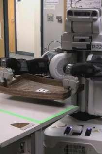
122 102 CHAPTER 6: ANYTIME E-GRAPHS (a) (b) (c) (d) Figure 6.4: The first, highly suboptimal path (a) (b) (c) (d) Figure 6.5: The final path

123 6.5 CHAPTER SUMMARY cells. The heading dimension is discretized into 16 directions. (a) E-Graph for an outdoor map (b) E-Graph for an indoor map Figure 6.6: Maps (x, y, θ) navigation experiments Our two methods were bootstrapped with 10 planning queries to build up an E-Graph with good coverage (Figure 6.6). Then, all methods were given the same 50 randomly generated test queries (E-Graph methods were not allowed to feed back the solutions to these queries so that they would have the same E-Graph throughout the tests). We compared our two methods against ARA*. The heuristic h G is a 2D Dijkstra search starting from the goal (this was also the heuristic used for ARA*). All methods planned to a first solution with a bound of 6 and were given two minutes total to plan, though optimality was generally reached much earlier than that. Figure 6.7 shows the average bound (across the 50 trials) reached over time. The optimal solution is generally found in the first 10 seconds for the outdoor map and within 30 seconds for the indoor map. We can see that H 2 has on par performance with H 1 even though it only computes the first E-Graph heuristic. The anytime profiles of our methods are actually slightly better than ARA* especially on the outdoor map. Examples of a first and final path for method H 2 on each map are shown in Figure Chapter Summary In this chapter, we have presented an anytime extension to planning with Experience Graphs. Anytime planners generate an initial solution quickly, which is typically suboptimal. Then, as additional time allows, they improve the solution quality until either the planning time expires or the optimal solution is reached. We discussed why anytime versions of planners are useful. One common situation is when the planner is allocated a time budget, such as when a planner is run in a repeatedly in a loop

124 104 CHAPTER 6: ANYTIME E-GRAPHS (a) Average bound over time on an outdoor map (b) Average bound over time on an indoor map Figure 6.7: Anytime profiles for (x, y, θ) navigation during the robot s execution. In this situation, we want the best possible path from the planner. However, at the same time we want to make sure some path is returned within the planning time (even if it is not optimal). While running something like A* (planning E-Graphs using a very low suboptimality bound) would produce a good path, we do not know how long it will take to find such a path and the time limit might expire before anything is found. Therefore, we instead start by finding any solution quickly by setting the E-Graph reuse bias very high, and then iteratively reducing it and replanning. This is more likely to always return some path, but still tries to use all the time to produce better solutions. We leveraged Anytime Repaired A* (ARA*) [56] in order to make an anytime variant of planning with Experience Graphs. Not only does this save quite a bit of repeated computation between iterations of the anytime algorithm, but it also provides a theoretical bound on the solution quality of the path after each iteration (better bounds after each). In our experimental analysis, we evaluated performance on full-body mobile manipulation pick-and-place tasks (both on the real PR2 robot and in simulation) as well as navigation. We saw that while ARA* and anytime E-Graphs improved solution quality at similar rates, E-Graphs found the first solution quicker and therefore got a head start in the improvement process. Compared RRT* (a sampling-based anytime algorithm) E-Graphs tended to have both faster planning times and better solution quality.

125 6.5 CHAPTER SUMMARY 105 (a) Outdoor first path (b) Outdoor final path (c) Indoor first path (d) Indoor final path Figure 6.8: Examples of anytime planning with the H 2 heuristic

126 106 CHAPTER 6: ANYTIME E-GRAPHS

127 Chapter 7 Planning with Experience Graphs in Dynamic Environments While planning with Experience Graphs performs best when environments are static, in practice, this is rarely the case. In this chapter, we explore ways to allow E-Graphs to perform better in dynamic environments as long as the changes are small. 7.1 Lazy Validation of Experience Graphs In this section, we leverage given experiences to tackle difficult planning scenarios where a robot s movement in a structured environment is encumbered by unpredictable clutter. Figure 7.1 shows a mailroom environment where the general task of sorting mail is a structured one. However, this environment typically has clutter appearing inside cubby holes or on shelves. By learning from experiences, we expect a mail-sorting robot to accumulate enough experience over time so that planning to constrained spaces (cubbyholes, boxes, etc) becomes very fast. At the same time, we expect this framework to be robust against the fact that portions of its given experiences are constantly becoming invalid due to clutter. In the absence of changing clutter, Experience Graphs provide fast planning times in this kind of challenging environment. The planner accumulates experiences throughout its lifetime by feeding back solutions. This results in faster planning times while maintaining completeness guarantees and a bound on the suboptimality of the solution with respect to the optimal path. While E-Graphs provide an efficient planning framework for a completely static environment with a large number of given experiences, planning times suffer once the possibility of unpredictable clutter is introduced. The E-Graph planner is only able to plan with a completely valid set of experiences; even a negligible change in the environment forces the planner to test for va- 107

128 108 CHAPTER 7: PLANNING WITH EXPERIENCE GRAPHS IN DYNAMIC ENVIRONMENTS Figure 7.1: PR2 in a simulated mailroom environment. lidity its entire set of experiences to ensure a valid plan. Considering the robot may be working tirelessly for long periods of time, the E-Graph can grow substantially and introduce more and more overhead into every single planning request. In this chapter, we address a question that affects any data-driven algorithm: does it scale? We describe efficient experience validation by introducing a general method that lazily validates experiences that the planner deems potentially relevant to the planning task. This method leads to performance improvements in changing, cluttered environments. Specifically, we show speedups using a simulated environment where the PR2 conducts single arm, 7D manipulation tasks in a constrained mailroom environment. In the following sections, we describe extensions to E-Graphs. In particular, we present the general method for lazy validation of E-Graphs, along with two possible design choices for its implementation (on-the-fly validation and post-validation). These two design options offer tradeoffs between speed and path quality (defined as the total length traveled by the end effector) and can be exercised when implementing a planner for a specific robotic domain. We present the post-validation version first to introduce the general idea of lazy validation, and then present the subtleties behind post-validation and on-the-fly validation Lazy Post-Validation Lazy post-validation is built on top of the original E-Graph planner described in Chapter 4; it uses the same heuristic computation to focus the search towards experiences. However, now instead of maintaining E-Graph feasibility and validity as an invariant, we loosely assume that the E-

129 7.1 LAZY VALIDATION OF EXPERIENCE GRAPHS 109 Graph is valid until the E-Graph planner returns a complete solution. Only then do we validate the vertices and edges in the solution path that lie on the E-Graph. During this validation, we also know that the only E-Graph edges that could be invalid are those used in the E-Graph shortcut - any other type of successor would be validated during the search. Algorithm 10 Planning with lazy E-Graphs 1: procedure LAZYPLAN(s start, s goal, G E ) 2: while not valid π do 3: initializeegraph(s goal ) 4: π = computep ath(s start, s goal ) 5: G E = G E π 6: (V invalid, E invalid ) = returninvalidelements(π) 7: G E = G E \ (V invalid, E invalid ) 8: if π = NULL and s start s goal then 9: return NO SOLUTION 10: else if s start = s goal then 11: return GOAL REACHED 12: else if E invalid = { } then 13: return π 14: procedure INITIALIZEEGRAPH(s goal ) 15: precomputeshortcuts 16: compute heuristic according to Equation 4.1 Algorithm 10 shows a high level overview of the logic for lazy post-validation. Given a prebuilt E-Graph G E, we run the standard procedure for E-Graph planning: initializing relevant E- Graph mechanisms (INITIALIZEEGRAPH), which pre-computes the shortcuts and the E-Graph heuristic. Once we compute a path π, we feed it back into the E-Graph in order to further accumulate experiences for later use. In returninvalidelements, we validate elements of G E related to π and return those that are invalid. In line 6, we remove these from G E, and rerun the planning cycle. Given that the E-Graph contains a sufficient amount of experience and the environment has not change dramatically, the number of total replans remains low. The goal of returninvalidelements goes beyond discovering points on the returned path that are invalid. Because the while loop continues to run until a valid path is returned, it is advantageous to discover as many invalid edges and vertices in G E as possible in a single run of returninvalidelements, especially those that are not explicitly part of π. In the ideal case, one could run a pre-computation to determine vertex connectivity in terms of the validation procedure. (i.e. return all V invalid given that a particular vertex is invalid). However, this is likely computationally expensive, so faster approximations can be used. In our implementation of lazy E-Graphs for robot arm planning, we check that the 3D location of the end effector for V ɛ invalid is not an obstacle. If it is, we look up all other V E that result in the same end effector position and invalidate those as well.

130 110 CHAPTER 7: PLANNING WITH EXPERIENCE GRAPHS IN DYNAMIC ENVIRONMENTS Figure 7.2: Three iterations of the post-validation method. While the plans are 7-dimensional, the pictures show their corresponding end-effector trajectories. The dark regions in the top two images show the invalid regions of the 7 DoF arm s path, while the dotted lines are the valid regions of the path. The last image shows a final (without shortcutting) path of the end effector.

131 7.1 LAZY VALIDATION OF EXPERIENCE GRAPHS 111 An example run of the post-validation method can be seen in Figure 7.2. Two replans are required before a completely valid path is found in the third image On-the-Fly Validation In the previous method, when a path was found, it needed to be checked for validity. The only parts of a path that could be invalid were the shortcut successors, which use the unverified E- Graph edges. In on-the-fly validation, we check the edges in a shortcut successor s shortcut (as described in Section 4.5.1) during the search as soon as the shortcut is generated. Therefore, when a path is found, it is guaranteed to be valid. There is no need to check for validity, and the loop in algorithm 1 is no longer needed Post-Validation vs. On-the-Fly Validation We now explore the subtle differences between these two implementations. As presented above, the post-validation algorithm validates the E-Graph paths only after a path has been successfully found. However, in certain domains, there can be substantial overhead in completely restarting the search (recomputation of heuristics, reinitializing data structures, etc.), especially if the environment changes drastically, resulting in many invalid E-Graph edges and many replans. On-the-fly validation avoids this overhead by validating the E-Graph edges during the search process. Specifically, this would occur whenever an E-Graph shortcut successor is generated. If the shortcut is found to be invalid, the successor is thrown out and the search proceeds in the standard fashion. This avoids the overhead problem associated with the post-validation method because the search does not have to restart when this occurs. However, the major caveat is that the E-Graph structure changes in the middle of the search. In the case where the E-Graph heuristic is pre-computed (which is the case for the implementations discussed in this thesis), there is now a potential problem for the heuristic to become extremely misinformed. This is illustrated in detail in Figure 7.3. We begin with two paths leading to the goal. When we introduce an obstacle that obstructs one of the experiences, a segment of the experience is taken out. At this point, we hope that the method will use the second path to the goal to quickly find a solution. Because the post-validation method reruns the heuristic computation every time the heuristic is invalidated, the search will be lead to the second path. However, the on-the-fly method s heuristic becomes uninformed because the heuristic is still drawn to follow the E-Graph as if the invalid segment is still connected to the goal. The correct choice between these two methods is very application dependent - if the overhead of recomputing the heuristic is negligible compared to overall planning time, then post-validation

132 112 CHAPTER 7: PLANNING WITH EXPERIENCE GRAPHS IN DYNAMIC ENVIRONMENTS Figure 7.3: A scenario where on-the-fly validation becomes highly inefficient due to a misinformed heuristic, whereas post-validation remains efficient. Before any invalidation occurs, the heuristic guides the search along the bottom path. When both methods discover that the experience passes through the obstacle, the corresponding edges are invalidated. Post-validation will recompute the heuristic and guide the search towards the top segment of experience. On-the-fly, however, will not recompute the heuristic, and will get stuck trying to bypass the obstacle. remains the better choice because the heuristic will be better informed and will result in higher path quality for the solution. However, if the average planning time is low enough that the overhead becomes significant, then on-the-fly validation can be used to improve planning times at the expense of success rate due to pathologically bad cases. In our experiments, these bad cases almost never occur Experimental Results We tested our approach in a simulated mailroom environment, where the PR2 robot is sorting objects between cubby holes, as seen in Figure 7.1. We use an existing benchmarking framework to run all experiments [15]. All the tasks involve manipulation with a single 7 DoF arm of the PR2. The goals are specified as the position and orientation of the end effector. We first build up a usable E-Graph by running 200 trials of random start goal pairs between the 18 cubby holes in the environment. These 200 trials are run with a very low bound (ε = 1.5) to ensure high quality experiences between locations. This results in an E-Graph of near 7000 vertices. Figure 7.4 shows a visualization of the E-Graph - each vertex represents the 3D location of the end effector of a particular V G and the edges represent end effector motions. For testing, we run 50 trials where each trial introduces six randomly placed obstacles in-

133 7.1 LAZY VALIDATION OF EXPERIENCE GRAPHS 113 Figure 7.4: An E-Graph with 7000 vertices. Each vertex represents the end effector location of a state, and edges represent the 3D movement of the end effector. side the cubbies. We plan using three different E-Graph based methods and the OMPL [18] implementation of the RRT-Connect. We do not report any results for Probabilistic Roadmaps or RRT* since they were both unable to successfully plan in this scenario. For the E-Graph based methods, we plan with a higher ɛ and ɛ E, allowing for more reuse of experiences. The choice of ɛ is based on the quality of the heuristic - when the heuristic well represents the planning problem, a low ɛ is acceptable. All paths undergo shortcutting in a post-processing phase. After each trial, the E-Graph is reloaded with the 200 trial training set. All statistics are computed on trials where all the planners succeed. We compare the two lazy validation (post and on-the-fly) methods with the naive solution: full validation. In full validation, we validate every vertex and edge in G E once a planning request has been received. This computation is factored into the planning time. In all algorithms, the validation of any E-Graph edge is equivalent to running a full collision check of the robot arm against the environment.

134 114 CHAPTER 7: PLANNING WITH EXPERIENCE GRAPHS IN DYNAMIC ENVIRONMENTS Post Full On-the-fly RRT-Connect Median CC/request Average CC/request Table 7.1: Collision check count comparison between three E-Graph methods and RRT-Connect. All E-Graph methods are initialized with an E-Graph of 7000 vertices. Post Full On-the-fly RRT-Connect Fast CC Medium CC Slow CC Success Rate 76% 80% 73% 84% Table 7.2: Average planning time in seconds using different speeds of collision checkers. The fast collision checker takes sec/collision check. The medium collision checker takes sec/collision check. The slow collision checker takes sec/collision check. As a reference, the SBPL approximate collision checker is the fast checker. The FCL collision checker is slightly slower than our medium collision checker at sec/collision check. The first experimental result we present is statistics on the number of collision checks that each planner issued. Because collision checking generally takes up a large portion of planning times, this offers an implementation-independent view of performance (compared to planning times, which depend on the particular collision checking implementation). Table 7.1 shows both the median and average number of collision checks for all planning methods. We see that the post and on-the-fly methods have lower average collision checks overall. We expect full validation to have a high average, because it is directly proportional to the number of E-Graph vertices. RRT-Connect has a difficult time in this environment, with an order of magnitude more collision checks due to the narrow passages from the cubbies. In order to get a sense of planning times, one experiment was run to demonstrate the planning times for different speeds of collision checkers. We begin with the SBPL collision checker, which operates very quickly because of its sphere-based approximate model of the robot [16]. However, in domains where a robot is manipulating objects, an exact collision checking model may be required, such as the Flexible Collision Library [63]. To get a sense of how the E-Graph methods scale with time required for a single collision check, we artificially increase the amount of computation in the SBPL collision checker to various speeds and measure the required planning time. Figure 7.5 shows a plot of the planning times, and Table 7.2 shows the times for several speeds of the collision checker. Overall, we see the clear relationship that, as collision checking time increases, full validation linearly increases

135 7.1 LAZY VALIDATION OF EXPERIENCE GRAPHS 115 Figure 7.5: A comparison between the post-validation and full validation method over different speeds of collision checking. These results were generated by artificially slowing the SBPL collision checker performance to various speeds. in planning time, while post-validation and on-the-fly validation do not suffer as much. As a reference, FCL takes roughly seconds per collision check. Interpolating on our results, FCL would spend about 12 seconds to plan for full validation, while post-validation still remains close to two seconds. The success rate for each method is calculated over the 50 test trials. We see that the on-the-fly is slightly faster in planning time than the post-validation method due to the reduced overhead associated with restarting a search and recomputing heuristics. However, in terms of path quality, on-the-fly does slightly worse, as seen in Table 7.3. This is expected, since the quality of the heuristic with the on-the-fly method is reduced as more E-Graph edges are obstructed by obstacles. Post Full On-the-fly RRT-Connect Average Path Quality Table 7.3: Path quality comparison between three E-Graph methods and RRT-Connect. All E- Graph methods are initialized with an E-Graph of 7000 vertices. In Figure 7.6, we show how the planning times for each method change with the size of the E-Graph measured by the number of nodes it contains. We see that, without the use of lazy

136 116 CHAPTER 7: PLANNING WITH EXPERIENCE GRAPHS IN DYNAMIC ENVIRONMENTS Figure 7.6: A comparison between the post, on-the-fly, and full validation methods over different sizes of E-Graphs. We see that the full validation method planning time increases linearly, while post and on-the-fly validation remain relatively constant. validation, the E-Graph planner does not scale well - planning times increase linearly with the size of the E-Graph. Post-validation and on-the-fly are on-par in performance, though vary with the randomness of the E-Graph Post-Validation vs On-the-Fly Analysis In the following experiment, we engineer a situation where on-the-fly fails, while post-validation succeeds. Here, a small set of experiences have been added to the environment, and the robot is planning from the top half of the cabinet to the bottom half. As explained before, the plan here fails due to structural changes in the E-Graph, which causes the heuristic to become misinformed. Specifically, we include a block that intentionally disrupts the original end effector path from the top to bottom of the block, which renders the heuristic useless, and the plan is unable to finish. In Figure 7.7, we introduce the obstacles, which disrupts the original experience. Figure 7.8 reflects the state of both algorithms after updating the E-Graph structure - with post-validation, this occurs once the full path has been found, and for on-the-fly, it happens during the search.

137 7.1 LAZY VALIDATION OF EXPERIENCE GRAPHS 117 Post-validation succeeds the second time after recomputing the heuristic, which generates the path seen in Figure 7.9. On-the-fly validation fails to plan because its heuristic continues to drive the search into the block, unaware that the environment has changed.

138 118 CHAPTER 7: PLANNING WITH EXPERIENCE GRAPHS IN DYNAMIC ENVIRONMENTS Figure 7.7: An existing E-Graph is disrupted by an obstacle. Figure 7.8: The E-Graph structure once both methods (post-validation and on-the-fly) have been updated to reflect the new environment. Figure 7.9: The post-validation solution, which succeeds because the heuristic is updated. Onthe-fly fails to plan in this situation.

139 7.2 INCREMENTAL E-GRAPHS Incremental E-Graphs In this section, we will discuss the application of Experience Graphs to incremental planning especially for high dimensional replanning scenarios. Incremental planners like D* [85] and D* Lite [47] are typically used when interleaving planning with execution. They are able to reuse computations from previous searches when the environment changes or when the starting state (the pose of the robot) changes. They do this by planning backward from the goal toward the start so that the root of the search tree is at the goal. When the start state changes, the entire search tree is unaffected and the planner just needs to keep running until the new start state is connected (it may even be in the search tree already). When the environment changes, some parts of the tree are invalidated. When changes happen near the leaves of the search tree (e.g. near the start state), these methods can typically reuse much of their prior search efforts. However, when changes occur near the root of the search tree (i.e. near the goal state), often very little can be reused. Sometimes determining what parts of the search tree were affected by a change can take a substantial amount of time and it can be faster to plan from scratch due to the bookkeeping needed to update g-values of states that are affected by changed edges in the graph. Because of this bookkeeping, existing incremental graph searches are not well-suited for planning problems that are higher than 3-4 dimensions. In contrast, E-Graphs are well-suited for high dimensional planning problems. (a) An initial plan to the goal. Here, the robot is shown at its start position as a circle. (b) After encountering a new obstacle (square object in figure), the planner reconnects the robot to the rest of the E-Graph by planning around the obstacle. (c) When the robot discovers an open door it thought was closed, h E guides the search through the door instead of continuing to follow the old path in order to stay within the suboptimality bound. It is able to reconnect with part of the E-Graph on the other side of the door. Figure 7.10: An example of using E-Graphs for incremental planning. E-Graphs can be used to plan incrementally with minimal bookkeeping and can still replan using prior computations even when both the start and goal states change. Unlike D*, which plans optimal paths, E-Graphs are only beneficial when searching for paths within a given sub-

140 120 CHAPTER 7: PLANNING WITH EXPERIENCE GRAPHS IN DYNAMIC ENVIRONMENTS optimality bound. E-Graphs handle incremental planning automatically just by feeding planned paths back into the E-Graph. Then if the start, goal, or both change, replanning is quick since the planner will just reconnect the states to parts of the E-Graph as long as it is within the bound on suboptimality the user provides. An experiment showing this kind of scenario is in our real robot experiments. E-Graphs also handle changing environments. When the environment changes, either of the lazy validation methods discussed in the previous section (Section 7.1) can be applied in order to minimize how much of the E-Graph is re-checked. For a sufficiently high bound, the planner will automatically repair the previous path if new obstacles broke the path. The planner will also shorten a previous path if an obstacle disappears, in order to stay within its suboptimality bound. To demonstrate how E-Graphs can be used to handle a changing environment, we give a small example in Figure Experimental Results We performed a proof of concept experiment demonstrating how E-Graphs can be used to do incremental planning. The experiment is on 10 DoF full-body planning for the real PR2 robot. The robot s task is to bring a tray to a person. The initial planning time is 8.15 seconds (with an empty Experience Graph). Figure 7.11a shows this first path. After the PR2 starts executing the path, the person slides down to the left side of the table and the goal state moves. The robot is told where the new goal is, stops, generates a new plan (Figure 7.11b) in 1.15 seconds, and finishes the task. The second planning time is short because the first path is now in the E-Graph and most of this path can be reused (only the end of the path needs to be modified). An interesting thing to note is that E-Graphs allowed previous computations to be reused even when both the start and goal states changed between the two planning requests. 7.3 Chapter Summary In this chapter, we discussed planning with Experience Graphs in dynamic environments. We stated early in this thesis that Experience Graphs work best when the environment is static. However, even in structured environments like warehouses, objects move and therefore, it is important that E-Graphs can still be used when there are changes. This chapter presented one approach to handling dynamic environments which assumes that changes in the environment are relatively small. For instance, when objects move on a table top, or the locations of packages in a mailroom. Our approached parallels the Lazy PRM. We assume the E-Graph is completely valid, plan a path, validate any edges in the path that came from the

141 7.3 CHAPTER SUMMARY 121 (a) Path to the first goal (b) Path to the goal after it moved Figure 7.11: Incremental E-Graph Experiment E-Graph, and then if any are not valid disable them in the E-Graph and plan again. The naive alternative to this lazy approach is to collision check the entire E-Graph before planning if the environment changed. In this chapter, we discussed a trade-off between these two methods. Our experiments on single arm planning in a mailroom show that the lazy method becomes more important as the E-Graph gets larger since checking up front becomes very expensive. However, if the collision checker is slower (high fidelity checks), it also becomes more beneficial to use lazy validation over full E-Graph validation upfront. Finally, we showed an application of E-Graphs to replanning scenarios. These are situations where a path is planned and then during execution, the planner is called again because a new obstacle was detected, the robot drove off the path, or the goal has changed. E-Graphs handles these situations naturally by simply keeping each generated path. When replanning, the algorithm will try to reuse as much of the previous path while staying within the set suboptimality bound. There are a number of other graph search algorithms which solve this problem, such as D*. They tend to have substantial bookkeeping that prevents them from performing well in high dimensional domains. High dimensional tasks are less of an issue when planning with E-Graphs. On the other hand, E-Graphs only provide bounded suboptimal solutions while D* provides optimal paths. Bounded suboptimal variants of D* exist, such as Anytime D* [55], which may perform the actual search quicker than D* in high dimensional spaces, but these methods must still perform the same substantial preprocessing (bookkeeping) to determine what states in the search tree were affected by environmental changes. Finally, an interesting qualitative difference

142 122 CHAPTER 7: PLANNING WITH EXPERIENCE GRAPHS IN DYNAMIC ENVIRONMENTS is how the location of environmental changes affects the planners. For most incremental planners (like D*), changes near the leaves typically require less work to repair than changes near the root. For E-Graphs, this makes little difference. Instead, it matters more if there is enough free space around the change to make a local repair to the path.

143 Chapter 8 Application to Assembly Domain Assembly is a well motivated task as it is performed in many factories. While automated assembly is used, it tends to be done with prescripted motions on expensive products like cars, which are produced in relatively high volume for an extended period of time. For these types of products, companies can afford to hand generate scripted motions for their manipulators. However, when looking at low volume production, or situations where very little time is given to set up production, assembly is often still performed by people. This is especially true for custom assemblies where only a few instances of a specific product will be produced. The domain we are interested in is assembly for custom objects where there are pre-made parts, and the robot s task is to attach them to each other. In addition to it being a useful problem, we believe this domain presents many opportunities to showcase Experience Graphs. In these tasks, new parts to be assembled come in from a constant small set of locations. Additionally, the robot s arms will continuously be visiting a central area where the product is being constructed. The fact that there is a small set of regions that the robot s end effectors travel between makes this an ideal task for reusing prior experience. Furthermore, in assembly tasks, while the robot is constantly using new pieces, the pieces will be instances coming from a small set of piece types. For instance, the robot may be working with many bolts or boards of certain dimensions. This means that the configuration space does not change in dramatic ways that the planner has not seen before. 8.1 Birdhouses The specific assembly domain chosen was constructing birdhouses (and other wooden objects of similar size like mailboxes). We imagine a scenario where people could design a birdhouse of their choice in CAD-like software and then send it to a company where a robot builds one (or a 123

144 124 CHAPTER 8: APPLICATION TO ASSEMBLY DOMAIN Figure 8.1: Examples of birdhouses. few) instance which is then shipped to them. Under this scenario, it would be too costly to handdesign trajectories for the robot to build this novel object. Therefore, if robots were desired to automate this task, they would need to generate their own motions to complete the construction. There were several reasons for choosing birdhouses for the set of objects. First, we wanted to choose a class of objects with a lot of variance in their design. The design of a birdhouse is up to personal preference and can be as varied as people s creativity Figure 8.1. The second reason was physical limitations of the robot we have access to. The PR2 robot has relatively weak arms and can only lift about 1-2 pounds when an arm is at full extension. Therefore, we had to choose objects that could be constructed from parts that were not too large or heavy (e.g. we considered furniture but this would have been too heavy). Conversely, perception limitations and the imprecision of the PR2 s arms would make assembling smaller objects too difficult (like constructing a matchbox or clothespin). 8.2 Task Setup and Hardware We assume that the pieces for the birdhouse the robot will assemble have already been cut out (Figure 8.2 shows pieces used for one of our birdhouses). The pieces are assumed to all be within reach of the robot, though if during the task the robot cannot reach a piece, it will ask a person to move it closer. We used a single parts table to hold all the pieces that will be used for the construction (though several surfaces could have been used). The pieces can be arranged in any way. In fact, we have many experiments with the pieces arranged in different ways. The parts table is labeled with a 1 in Figure 8.3. The PR2 will pick up pieces with its left arm using a vacuum gripper (Figure 8.4 and item 2 in

145 8.2 TASK SETUP AND HARDWARE 125 Figure 8.2: Various pieces used to assemble our birdhouses. Figure 8.3: The birdhouse assembly setup. Item 1 shows the parts table where pieces used to build the house are arbitrarily placed. Item 2 is the vacuum gripper the PR2 uses to pick up pieces. Item 3 is the work table which the robot builds the house on top of. The work table has a suction cup which holds the house down. The table also has a servo inside so the robot can command the table surface to rotate. Item 4 is the nailgun the robot uses to attach pieces.

146 126 CHAPTER 8: APPLICATION TO ASSEMBLY DOMAIN Figure 8.4: The vacuum gripper the robot uses to pick up pieces. The robot s fingertips fit snugly into the grooves on the black block on the left. The suction cup on the right picks up the pieces. The robot can turn the suction on and off. When a piece is picked up, the suction cup compresses inward and the piece is held against the green plastic bowl, which keeps the piece rigid. Without this plastic, the rubber suction cup could flex. Figure 8.3). The robot can turn suction on and off using a valve it can control through an arduino. We found the vacuum gripper to pick up pieces much faster than using the robot s pincher and provided solid grasps. It also made it very easy to generate a large set of valid grasps for pieces. The assembly is built on the work table (Figure 8.5 and item 3 in Figure 8.3). The worktable acts as a third hand for the robot. It has another suction cup (which the robot can also turn on and off) which is used to hold the base of the birdhouse down to its surface while the robot attaches new pieces to it. Additionally, the top of the work table (and suction cup) can rotate using a servo motor inside. The PR2 can control the servo as well and can use this ability to spin the birdhouse in order to make different sides easier to reach during construction. When the robot has moved a piece into place, it attaches it to the current structure with nails. We built a custom nailgun built for the robot which it can grip easily (Figure 8.6). The internals of the nailgun come from an off-the-shelf electric nailer. A new casing was 3D printed to include notches which the robot s fingers fit snugly into. The nailgun is held in the robot s right gripper (item 4 in Figure 8.3). The PR2 is able to fire the nailgun via an arduino. Additionally, there is a button near the muzzle of the nailgun which the robot gets feedback from. This allows the robot to make sure it only fires the nailgun if it is making contact with a surface. On the software side, the robot is given geometric models of all the pieces (for collision checking), a list of possible grasps for each piece (typically per piece), the poses of all the

147 8.2 TASK SETUP AND HARDWARE 127 Figure 8.5: The birdhouses are build on top of this wooden cylinder, called the work table. Notice the suction cup on top which which the robot can turn on and off. The suction allows the robot to hold the house down while it is being built. The top section of the work table (the dark part of the cylinder) can be rotated using a servo which is contained inside the bottom section (light part of the cylinder). The robot can control the angle of this servo. Figure 8.6: The nailgun casing was custom made in a 3D printer. The internals of the nailgun are from an off-the-shelf electric nailer. The robot can fire the nailgun by wire. The robot s fingertips fit snugly into the dark-colored rectangular notches in the middle of the nailer (only one of the two notches is visible, the other is underneath). The metal rectangle on the right holds the nails and the nails shoot out the upper right corner (firing in the rightward direction). A small metal tab sticks out the upper right corner which is connected to a button that tells the robot when it is in contact with a surface.

148 128 CHAPTER 8: APPLICATION TO ASSEMBLY DOMAIN Figure 8.7: Several examples of AR Marker fiducials. Each marker encodes a unique identification number. Using a camera, the robot can estimate the position, orientation, and identification number of these markers. pieces in the birdhouse (all relative to a designated base piece), and the locations of all the nails. 8.3 Software modules This project required many software modules including those related to motion planning. This section will describe the various modules and a brief idea of how they were implemented Perception All perception for the project was done with the aid of fiducials, specifically, AR Markers (Figure 8.7). Using a ROS package (ar track alvar), the robot can estimate the position and orientation of each of the tags in view. Additionally, each tag encodes an identifying number which the robot can read as well. By attaching these tags to each of our pieces, we can estimate their pose in the world as well as identify which piece is being seen (we can then associate that piece s geometric model with it). We found through experimentation that while there is some noise in the position estimation (< 1cm), the estimation of the orientation can be much worse, sometimes up to 90 degrees off. We therefore sought to improve the estimation of the orientation. We decided to use bundles of markers, which are patterns of markers the user can lay out. The robot is told the transform from each of the markers in the pattern to some chosen bundle frame and therefore, when the robot see several of the markers simultaneously, it can make better estimates for the pattern as a whole. The ROS package, ar track alvar already has the ability to do bundle tracking. However, it incorporates both the positions and orientations of the markers in order to have each visible marker provide its own estimate of the bundle frame, and then averages these estimates. This works well when the noise is small. However, if there is significant orientation error in a marker that happens to be far from the bundle frame, it will result in that marker providing an

149 8.3 SOFTWARE MODULES 129 Figure 8.8: An example of the bundle tracking detecting pieces in an image. estimate for the bundle frame which has large position error. When averaged with the estimates from the other markers, this outlier can skew the average. We improved this by implementing our own version of bundle tracking, which ignores the orientation estimates of the individual markers and only uses the position estimates. The pose of the bundle frame can then be found by finding a rigid transform from the set of points in the known pattern and the set of points currently being seen. Since we know the correspondences between the two sets of points (the AR Markers encode an identifying value), we can find the rigid transform that minimizes the squared error between the points using SVD [7]. We found that this implementation of bundle tracking works significantly better in practice. We attached these bundles to both sides of each piece that the robot would be using. We incorporated some additional domain knowledge to improve accuracy. For instance, we knew that the pieces would be lying flat (either face-up or face-down) on a table. Therefore, we can adjust the orientation to the nearest of those two cases while maintaining the same yaw (lying flat tells us nothing about the yaw of the piece). Figure 8.8 shows several pieces and the detections found by bundle tracking. We also attached these bundles to important objects in the environment. For instance, the parts table had one of these patterns on it. By knowing where the parts table is located, we can be sure to generate motion plans which do not run into it, but it also informs the robot where it should scan to look for available pieces. The work table also has markers placed on it which ensure we do not collide with it and also tells the robot where it should assemble the birdhouse.

150 130 CHAPTER 8: APPLICATION TO ASSEMBLY DOMAIN Figure 8.9: Examples of possible grasps for a piece High-level planning Each birdhouse is constructed with a number of instructions or steps. Each instruction involves attaching another piece onto the house and possibly putting some number of nails into that piece to hold it on (the first piece does not have any nails as there is nothing to attach it to). To complete each instruction, a number of discrete decisions must be made and motion plans generated. For any given instruction, the first decision is piece selection. Suppose the next piece to be attached is a 6 by 6 square. It may be that there are 3 such pieces of the exact same type (shape and dimensions) used in the birdhouse. Therefore, the robot can choose from any of these piece instances. The next discrete decision is which grasp to use to install the piece. Each piece has around grasps which are typically in 5 or 6 different locations on the surface of the piece. Each has 8 different possible yaws of the suction cup. Figure 8.9 shows two possible piece grasps. The third discrete decision is the work table orientation. Recall that the work table can be rotated to make the attaching easier. A reasonable guess for the needed angle is made by looking at where the piece needs to be attached in the structure and choosing an angle which puts this location as close to the robot s body as possible. Then, several angles (usually about 3-4) in the neighborhood of this angle are options that can be used in the upcoming step. At this point, enough discrete decisions have been made to pick up the piece and put it in place. Therefore, the remaining choices involve putting in nails. The fourth decision to be made is which nail from this piece will be put in first. The first nail is different from all the others. After the first nail has been installed, the vacuum gripper can safely release the piece because it will stay in place on its own. This makes the nails after the first one much easier to install. However, the first nail needs to be put in while the vacuum gripper is still holding the piece in

151 8.3 SOFTWARE MODULES 131 Figure 8.10: When the first nail for a piece is put in, both the vacuum gripper and nailgun need to be near the piece, making it crowded. The choice of which nail to put in first can make this much easier (or even feasible). place, making it much more crowded since both the vacuum gripper and nailgun will be very close to one another (Figure 8.10). The final discrete decisions are the rolls of the nailgun for each of the nails for this piece. A nail is rotationally symmetric about the axis that runs from head to tip (roll). Therefore, the nailgun can be rotated about this axis and the result of the nailing will be the same. However, certain choices of the nailgun roll will be easier due to arm kinematics and proximity to the environment. One obvious discrete decision that I did not mention was choosing the order that the pieces should be assembled in. In order to make the problem a bit simpler, we decided to have the user specify this order in advance. It would be interesting to remove this assumption in the future. We chose to approach the birdhouse assembly problem as a two-level planning problem. A high-level planning phase makes all the discrete decisions while a low-level motion planner validates that those decisions are valid and can be executed. If the motion planner fails, the highlevel planner makes different choices which may have better success. This is called hierarchical planning. Performing hierarchical planning in a principled manner is a research challenge that a number of people have looked at [84, 39]. Our particular high-level planning problem is not as complicated as the ones tackled by these cited works which can handle combining symbolic planning with motion planning. Our problem only involves selecting a valid assignment to a set of variables. This is known as a Constraint

152 132 CHAPTER 8: APPLICATION TO ASSEMBLY DOMAIN Figure 8.11: The Constraint Satisfaction Problem being solved for our assembly task can be visualized as a decision tree. The solver we implemented tries to search from the root to a leaf (assign all variables), and then validate the assignment with motion planning. A number of simpler validations are done at intermediate nodes in the tree in order to prune branches before they are searched. Satisfaction Problem (CSP). We created a simple solver which iterates over the possible assignments of values to each of our discrete variables and then invokes the motion planners (using E-Graphs) for validation. Specifically, the variables in our CSP are: The piece to use for the upcoming attachment step if there are several remaining instances of the same piece type. (usually 1-3 options) The grasp to use for installing the piece. (usually options) The angle the work table should be rotated to. (usually 3-4 options) Which nail will be put in first. (usually 2-6 options) For each nail, what roll should nailgun use. (usually 2-6 variables, each having 6 options) The CSP can be viewed as a tree structure (Figure 8.11) where each variable represents a layer in the tree. Moving from the first layer to the second represents choosing a value for the first variable. Therefore, the branching factor at the first node is the number of values the first variable can take. Moving from a node in the second layer to the third layer means choosing a value for the second variable, and so on. Clearly, the size of the tree (and number of assignments) is exponential in the number of variables. In order to accelerate finding a valid assignment, there are number of pruning rules that can be used to cut branches off of this search tree at shallow depths which prevent searching over large sets of assignments.

153 8.3 SOFTWARE MODULES 133 Most of these pruning rules make use of domain knowledge. For instance, once a piece and grasp have been chosen, the process of picking up the piece can be validated without having to choose values for any other variables. If this passes, the work table angle is chosen and then validation can be run (without assigning any other variables) to see if the piece can be held at the put down pose in the structure. If these checks were to fail, it means that entire branch of possibilities can be pruned away. Another example of a simple check is not allowing a selection of a first nail which happens to be very close to the chosen grasp since this would mean that the gripper holding the vacuum gripper would come into collision with the gripper holding the nailgun. Many of the checks used involve running inverse kinematics, such as: to see if it is possible to put the vacuum on the piece for pick up, hold the piece in the put down position in the structure, or hold the nailgun at each of the nail poses. While there are many of these inverse kinematics feasibility checks that are used directly in the CSP-solver, we do not actually use motion planning to validate anything until all variables have been assigned (since IK calls are much cheaper than planning). Then, all motion plans are generated (pick up, put down, nailgun motion, etc). If any of the plans fail, the CSP solver is told to try another assignment Motion planning The motion planning problem needs to be solved constantly in an assembly task. As discussed earlier, since the environment changes very little and the robot is moving its tools between a small set of regions, it makes this task ideal for experience reuse. Now that more details have been given about our birdhouse assembly domain, we can see that the vacuum gripper will be moving to various places over the parts table to pick up pieces, and then to a region around the work table. The nailgun also travels to locations around the work table and then to a position off to the side (to get out of the way). We can clearly see that each arm is traveling between two regions repeatedly. E-Graphs should do very well in this situation. We ran two different 7DoF arm planners (for the left and right arm). Each is planning in joint space for its arm [16]. The heuristic for the planner is a 3D Dijkstra search which guides the wrist toward the goal position of the wrist. We use Experience Graphs on top of this, making use of the fast implementation possible when the domain-specific heuristic is computed by dynamic programming (Section 4.6). Figure 8.12 shows an example of the E-Graphs for the left and right arm after building a birdhouse. The motion planners are called from the CSP-solver described in the previous section. They are used to validate the high-level plan for attaching the next piece to the structure. Recall, that the CSP-solver will probably try many assignments before finding one that is valid with respect to

154 134 CHAPTER 8: APPLICATION TO ASSEMBLY DOMAIN Figure 8.12: A visualization of the E-Graphs for each arm after constructing a birdhouse. The red line segments show the edges while blue dots are the vertices. In order to not clutter the image, the states and edges of the E-Graph (which are 7 DoF) are shown as down-projected points in 3D which represent the location of the wrist. all constraints and motion plans. This presents a unique opportunity to reuse experience. When the CSP-solver validates one phase and it succeeds (like picking up the piece) but then a later phase fails (like moving the nailer to put in the first nail), the plan generated from that first phase is saved, even though other plans did not succeed. When another assignment is tried, E-Graphs allows the validation to be much faster. If the piece and grasp did not change, the plan is just recalled. If the grasp changed, it is typically a small change to adapt the previous trajectory to move to the new grasp Dealing with imprecision A major challenge we encountered while getting the PR2 to build birdhouses was dealing with the large amount of imprecision in the arms and cameras. Even after performing the PR2 s calibration procedures [76], we found the robot s ability to put its end effector at a point it looked at could be off by up to 2cm. For many common manipulation tasks, like picking up objects and moving them to other places, this level of inaccuracy is acceptable. When using a pinch grasp, the gripper is often wider than the object by a margin larger than 2cm. Therefore, the gripper can still fit around the object and grasp it. Even with a vacuum gripper, if our only task was to pick up the pieces, we could always use grasps that were more than 2cm away from any edge and this amount of error would be acceptable. However, this amount of imprecision is too much for meshing two pieces of wood together to

155 8.3 SOFTWARE MODULES 135 form a square joint. Therefore, there were several modules we used in order to reduce the error to within a millimeter. We added several components to the system in order to mitigate the effect of imprecision: correction libraries, a piece alignment behavior, visual confirmation, and a nailgun alignment behavior. Correction Library The optimization performed in the calibration routine tries to fit the parameters of a model to minimize the error across all possible locations that we may see and want to grasp in the robot s workspace. We noticed that this meant some regions of the workspace had smaller error than others (i.e. when looking at a marker and trying to touch it with the end effector, the robot got closer to the mark in some regions than in others). We also noticed that the error was generally consistent (i.e. the error in the position of the end effector was usually similar when the marker was put in different places within a small region). Therefore, we thought we could apply a region based correction when moving the end effector to something perceived visually. We did this by having the robot repeatedly reach for a marker which we would move around. When there was error, we would provide a kinesthetic demonstration by moving the robot s hand to the proper place. The robot would record the error vector between where it thought it should go and where the human put the gripper, and then the robot could use this correction in the future when it was near this correction. We used a simple 1 Nearest Neighbor lookup to predict the correction for a novel location (Gaussian Process Regression may have been useful if we had noticed more noise in the data). After collecting a number of corrections on both the parts table and work table, we saw some improvement. The error on picking up pieces was usually within 1cm. Figure 8.13 shows a visualization of the correction library for the left arm. The small spheres over the table are shown in pairs indicating where the end effector was placed and then where it was corrected to. The green pair of spheres is a query point where the robot would like to put the vacuum and a corrected location automatically generated from finding the nearest neighbor in the correction library (the red pair of spheres). Piece alignment behavior The part where the error is the biggest problem is meshing the pieces together. This is because, while there is still error in putting a piece down, there was also error in picking the piece up. This means that the piece is not exactly in the gripper where the robot thinks it is, resulting in compounded error.

156 136 CHAPTER 8: APPLICATION TO ASSEMBLY DOMAIN Figure 8.13: The correction library for the left arm in the assembly domain. In order to eliminate the error, we developed a behavior which can detect contact between the piece and the structure. We then used this in a sequence of motions to reduce the error to a negligible amount for our task (typically within a millimeter). The behavior is run once the robot believes it has moved the piece to within a few centimeters of contact. The behavior is best illustrated with an example, as shown in Figure Imagine trying to attach a vertical wall to the base of the birdhouse. The placement procedure works by intentionally starting the piece too far back and too low. We then move the piece forward in small steps by running inverse kinematics for a piece pose with the same orientation, but with the position that is slightly closer to the structure. We move the piece forward with these small steps until contact is detected between the piece and structure. We then move the piece upward in small steps until contact is not detected in front of the piece. This means that the piece has risen above the base piece. At this point, we again move the piece forward until contact. We designed the pieces to have a stair-step edge so that the pieces fit together more snugly (Figure 8.14). This also allows the robot to move the piece forward this second time and expect to have contact again. Once this happens the piece is pushed forward and down a bit in order to make a snug fit. Then nails are put in. One important detail to this procedure is how contact is detected. We do not have any sensors on the pieces and therefore we don t have any direct means of measuring contact. We instead detect contact by measuring the workspace error in the end effector. Specifically, if we

157 8.3 SOFTWARE MODULES 137 Figure 8.14: All pieces used in the structure have a stair-step around their edge. This allows pieces to fit together snugly. (a) The piece starts back and below the edge. (b) The piece moves forward until contact. (c) The piece moves up until no contact. (d) The piece moves forward until contact. Figure 8.15: The behavior used to put pieces into place.

158 138 CHAPTER 8: APPLICATION TO ASSEMBLY DOMAIN wanted to test for contact in the positive x-direction in the held piece s frame (let s say this is the direction that moves the piece toward the structure). Then we take the current piece s pose, increase its x-coordinate by a small amount, and run inverse kinematics to get joint angles that would put the piece at this pose. We then send these joint angles to the arm controller. After the joint angles are no longer changing, one of two things has happened. Either the controller reached the desired goal or a collision occurred which prevented the controller from reaching the goal. Which of these two cases it is can be determined by taking the current joint angles of the arm and running forward kinematics to get the current pose of the piece. If the current pose is very close to the desired pose, then the test for contact failed (as we did not hit anything). If there is substantial error, this implies that contact was made. We then use the ability to detect contact or lack of contact in the behavior described above. Visual confirmation The above described behavior works well at seating new pieces into the structure even if the point grasped on the piece is off from where was desired. However, the behavior only corrects for position error. If the piece is yawed on the vacuum gripper, it can cause the behavior to fail. This is because the piece will never sit flat on the edge in the structure we are trying to attach it to. Therefore, before trying to install the piece, the robot will hold the piece up in front of its cameras and observe the locations of the AR Markers on the underside of piece (Figure 8.16). This lets the robot estimate the error it had when it picked up the piece off the table. Any yaw error that is detected can then be removed by rotating the piece when we start the behavior discussed above. This method worked very well at detecting yaw error, which we attribute to holding the piece closer and straight on to the camera, as opposed to the view the robot gets when the piece is on the parts table. This visual check has the added benefit of confirming that the piece was picked up at all as the robot has no other way of telling if it missed the piece. Nailgun alignment behavior We designed a similar procedure (Figure 8.17) to the one used for installing pieces in order to putting in nails. The nailgun however, has a small button at the muzzle that makes it substantially easier to detect contact. If a nail was trying to be put in along the bottom edge of the birdhouse, we first start with the nailgun artificially high and back. The robot then moves the nailgun forward until contact is detected. Then, it moves the nailgun down until no contact is detected. At this point the nailgun is just below the bottom edge of the birdhouse. We then move it back up until contact is detected again and fire the nail.

159 8.4 EXPERIMENTS 139 Figure 8.16: After picking up a piece, the PR2 looks at the piece to determine the error in the grasp. 8.4 Experiments In order to evaluate the performance of E-Graphs for motion planning, as well as the system as a whole we ran a number of experiments. We built several birdhouses with the real robot and then built much larger and more interesting houses in simulation experiments Real Robot The real robot experiments test the entire assembly process (all modules described above). The birdhouse we had the robot build is shown in Figure This birdhouse is built from 6 pieces of wood and 12 nails. The robot constructed 5 instances of this house (Figure 8.19 shows 3 of them). An additional unexpected constraint we found during our experiments was that the robot could not lift the nailgun too high due to its weight. Unfortunately, this meant that the birdhouse we would construct in real life could only have one floor and that putting nails into the roof was very unreliable. Therefore, the robot attached the roof of each of these houses with velcro. Table 8.1 shows the amount of time spent on each instruction of the birdhouse. Prep time includes scanning the parts table to find the piece needed for this step, running the CSP-solver, generating all motion plans, and shortcutting paths. Execution time includes executing all motions to rotate the work table, to pick up the piece, perform visual confirmation, move the piece to the work table, execute the piece meshing behavior, install all nails (using nail alignment behavior), and move each arm back to its home configuration. The first and last instructions take the least amount of time to execute since these steps do not have any nails (the first piece has nothing to attach to and the last piece is the roof, attached with velcro). In fact, the piece meshing

160 140 CHAPTER 8: APPLICATION TO ASSEMBLY DOMAIN (a) The nailgun starts back and above the edge. (b) The nailgun moves forward until contact. (c) The nailgun moves down until no contact. (d) The nailgun moves up until contact. Figure 8.17: The behavior used to algin the nailgun with the piece edge. Figure 8.18: The visualization of a desired birdhouse and an actual instance of the birdhouse constructed by the PR2.

161 8.4 EXPERIMENTS 141 Figure 8.19: Several of the birdhouses the PR2 built (3 of 5 shown). Table 8.1: Time spent on each instruction during real birdhouse assembly mean std mean std mean std prep prep execution execution total total instruction time(s) time(s) time(s) time(s) time(s) time(s) behavior and nail alignment behaviors consume the vast majority of the birdhouse construction time. Therefore, with a more precise arm we may be able to achieve much lower construction times. On average it took seconds (20 minutes) to complete the entire construction, with a standard deviation of 106.1s. Figure 8.20 shows the full construction of one of the birdhouses Simulation Our simulation experiments are used to build many more and creative birdhouses. They also more rigorously test the motion planners and E-Graphs. In simulation, perception and behaviors that deal with imprecision were not tested. The robot is told exactly where the pieces and tables are in the world and the robot is capable of moving its end effectors exactly where it wants to. Therefore, these experiments primarily test the CSPsolver and motion planners.

162 142 CHAPTER 8: APPLICATION TO ASSEMBLY DOMAIN Figure 8.20: This sequence of images shows the construction of one of the birdhouses.

163 8.4 EXPERIMENTS 143 (a) 6 pieces, 14 nails (b) 12 pieces, 40 nails (c) 6 pieces, 18 nails (d) 5 pieces, 14 nails (e) 11 pieces, 36 nails (f) 5 pieces, 12 nails Figure 8.21: The different birdhouses constructed in our simulation experiments and how many pieces each used Six different types of birdhouses were constructed and each was built 10 times where the pieces were arranged differently between each of the runs. Figure 8.21 shows the six types of houses constructed. As mentioned earlier, since the robot has a difficult time lifting the nailgun above a certain height, some of the houses shown here would have been impossible to construct with the real robot unless the nailgun were lightened. The results shown in Table 8.2 show how the CSP-solver performed across all assembly tasks. This table shows each of the decisions that the CSP-solver must make. Piece refers to choosing a piece when there are multiple instances on the table. Grasp refers to which grasp is used to pick up the piece. Work table angle refers to what angle the work table is rotated to for this instruction. First nail refers to which nail is chosen to put in first while first nail roll is what roll the nailgun uses for that nail. Other nail rolls refers to the choice of roll for