Applying vessel inlet/outlet conditions to patientspecific models embedded in Cartesian grids
|
|
|
- Lizbeth Logan
- 5 years ago
- Views:
Transcription

 thesis, University of Iowa, 2015. https://doi.org/10.17077/etd.6yjl67sm Follow this and additional works at: https://ir.uiowa.")
1 University of Iowa Iowa Research Online Theses and Dissertations Fall 2015 Applying vessel inlet/outlet conditions to patientspecific models embedded in Cartesian grids Aaron Matthew Goddard University of Iowa Copyright 2015 Aaron Matthew Goddard This thesis is available at Iowa Research Online: Recommended Citation Goddard, Aaron Matthew. "Applying vessel inlet/outlet conditions to patient-specific models embedded in Cartesian grids." MS (Master of Science) thesis, University of Iowa, Follow this and additional works at: Part of the Biomedical Engineering and Bioengineering Commons
2 APPLYING VESSEL INLET/OUTLET CONDITIONS TO PATIENT-SPECIFIC MODELS EMBEDDED IN CARTESIAN GRIDS by Aaron Matthew Goddard A thesis submitted in partial fulfillment of the requirements for the Master of Science degree in Biomedical Engineering in the Graduate College of The University of Iowa December 2015 Thesis Supervisor: Associate Professor Sarah C. Vigmostad
3 Graduate College The University of Iowa Iowa City, Iowa CERTIFICATE OF APPROVAL This is to certify that the Master s thesis of MASTER S THESIS Aaron Matthew Goddard has been approved by the Examining Committee for the thesis requirement for the Master of Science degree in Biomedical Engineering at the December 2015 graduation. Thesis Committee: Sarah C. Vigmostad, Thesis Supervisor H.S. Udaykumar Madhavan Raghavan Edward Sander Jia Lu
4 To my wife and family for all their love and support. ii
5 ACKNOWLEDGEMENTS I would like to thank my advisors, Associate Professor Sarah Vigmostad, and Professor H.S Udaykumar for their guidance and opportunity to create this body of work. I would like to thank my wife, Amanda, and my family for their love and continued support during my education. I would also like to thank lab mates Nirmal, Oishik, Liza, Moustafa, Ehsan, Mike, Sidhartha, Pratik, Kayley, and Jared for creating an enjoyable work environment. iii
6 ABSTRACT Cardiovascular modeling has the capability to provide valuable information allowing clinicians to better classify patients and aid in surgical planning. Modeling is advantageous for being non-invasive, and also allows for quantification of values not easily obtained from physical measurements. Hemodynamics are heavily dependent on vessel geometry, which varies greatly from patient to patient. For this reason, clinically relevant approaches must perform these simulations on patient-specific geometry. Geometry is acquired from various imaging modalities, including magnetic resonance imaging, computed tomography, and ultrasound. The typical approach for generating a computational model requires construction of a triangulated surface mesh for use with finite volume or finite element solvers. Surface mesh construction can result in a loss of anatomical features and often requires a skilled user to execute manual steps in 3rd party software. An alternative to this method is to use a Cartesian grid solver to conduct the fluid simulation. Cartesian grid solvers do not require a surface mesh. They can use the implicit geometry representation created during the image segmentation process, but they are constrained to a cuboidal domain. Since patient-specific geometry usually deviate from the orthogonal directions of a cuboidal domain, flow extensions are often implemented. Flow extensions are created via a skilled user and 3rd party software, rendering the Cartesian grid solver approach no more clinically useful than the triangulated surface mesh approach. This work presents an alternative to flow extensions by developing a method of applying vessel inlet and outlet boundary conditions to regions inside the Cartesian domain. iv
7 PUBLIC ABSTRACT Cardiovascular modeling has the capability to provide valuable information allowing clinicians to better classify patients and aid in surgical planning. Modeling is advantageous for being non-invasive, and also allows for quantification of values not easily obtained from physical measurements. Fluid flows are heavily dependent on vessel geometry, which varies greatly from patient to patient. For this reason, clinically relevant approaches must perform these simulations on individual patient geometry. Geometry is acquired from various imaging methods including MRI, CT, and ultrasound. The typical approach for generating a computational model requires construction of a triangulated surface mesh for use with finite volume or finite element solvers. Surface mesh construction can result in a loss of anatomical features and often requires a skilled user to execute manual steps in 3rd party software. An alternative to this method is to use a Cartesian grid solver to conduct the fluid simulation. Cartesian grid solvers do not require a surface mesh. They can use the geometry representation created during the image segmentation process, but they are constrained to a box shaped domain. Since individual patient geometry usually deviate from the perpendicular directions of a boxshaped domain, flow extensions are often implemented. Flow extensions are created via a skilled user and 3rd party software, rendering the Cartesian grid solver approach no more clinically useful than the triangulated surface mesh approach. This work presents an alternative to flow extensions by developing a method of applying vessel inlet and outlet boundary conditions to regions inside the Cartesian domain. v
8 TABLE OF CONTENTS LIST OF TABLES... viii LIST OF FIGURES... ix CHAPTER 1 INTRODUCTION Applications of computational modeling in the cardiovascular system Challenges of patient-specific modeling in the clinical environment Challenges with the conventional approach to Cartesian domain boundaries Proposed alternative Interior boundary conditions... 6 CHAPTER 2 METHODS Specific features of the selected computational framework Comparison of Cartesian grid construction Defining interior boundary cap parameters Locating the boundary cap endpoints Cell reclassification Ghost Fluid cell classification Flow solver modifications Time splitting method Modification to the gradient scalar calculation Modification to the convection calculation Modification for extrapolation to boundary Modifications for the Dirichlet boundary condition Global mass conservation Modifications to the outlet boundary condition Modification to the Helmholtz equation Modification to the divergence calculation Modifications to the Pressure Poisson equation CHAPTER 3 VALIDATION Validation of Poiseuille flow Validation of 2D aortic arch with commercial software CHAPTER 4 EMPLOYING INTERIOR BOUNDARY CAPS TO MODEL IMAGE- BASED GEOMETRY Image-to-flow on patient-specific data vi
9 4.2 Other image-to-flow uses Image-to-flow on computer drawn image Image-to-flow on hand drawn image CHAPTER 5 CONCLUSIONS Summary Limitations and future work REFERENCES vii
10 LIST OF TABLES Table 1: Comparison of boundary cap max to the analytical value viii
11 LIST OF FIGURES Figure 1: Example of a typical physiologic geometry which fails to conform to a Cartesian domain Figure 2: Flow extensions for conventional domain boundaries. (a) 2D representation of idealized aorta geometry (b) Idealized aorta with flow extensions that would be traditionally required to perform flow computation on Cartesian grid solver Figure 3: Illustration of cells near the desired interior boundary cap being inserted into the conventional domain arrays for purposes of applying vessel inlet/outlet boundary conditions Figure 4: Comparison of computational domain construction between (a-d) conventional domain boundary conditions and (e-h) interior boundary caps. (a,e) set up initial grid and insert geometry, (b,f) prune mesh and apply boundary caps, (c,g) refine mesh and classify cells as fluid/solid, (d,h) perform flow simulation Figure 5: Some of the new geometric configurations interior boundary caps allow. The fluid domain is marked in dark gray. (a) Entire geometry inside the domain, (b) All inlets/outlets crossing domain boundaries, (c) Combination of each, (d) Interior boundary caps used with conventional domain boundary conditions Figure 6: Comparison of how boundary conditions cells are selected (a-c) conventional domain boundaries (d-f) interior boundary conditions, (a,d) initial grid, (b,e) insert geometry and reclassify outside cells as solid, (c ) level set values are used to identify domain boundary cells, (f) level set values and boundary cap plane are used to identify boundary cap cells and cells outside the place are changed to solid Figure 7: Differences between conventional domain boundary cells (a-c) and interior boundary cap cells (d-f). (a,d) boundary cell spacing, (b,e) flux contribution to neighbors, (c,f) boundary condition normal Figure 8: Linear extrapolation to boundary. Interpolation between the encircled cells is used to determine values of the probe points (solid black circles) Figure 9: Dirichlet boundary condition projection for interior boundary conditions Figure 10: Calculation of mass flux using stair step method Figure 11: Helmholtz equation stencil of coefficients for interior cells ix
12 Figure 12: Helmholtz equation stencil of coefficients for boundary adjacent cells (a) conventional domain boundaries (b) interior boundary conditions Figure 13: Pressure Poisson equation stencil of coefficients for interior cells Figure 14: Pressure Poisson equation stencil of coefficients for west boundary adjacent cells (a) conventional domain boundaries, (b) typical interior boundary conditions, (c) stair step interior boundary conditions Figure 15: Neumann conditions for construction of the Poisson operator matrix at boundary adjacent cells noted by a plus, (a) typical boundary adjacent stencil including a single boundary neighbor, (b) indication of cells needed to apply substitution for boundary cell, (c) boundary adjacent stencil at stair step showing two boundary neighbors, (d) boundary adjacent stencil for stair step cell for substitution of boundary cells Figure 16: Velocity magnitude comparison (Re = 100) using pelafint3d with interior boundary caps (top) to pelafint3d using conventional domain boundaries (bottom) Figure 17: Poiseuille flow validation at Re = 100. (top) longitudinal centerline velocity, (bottom) fully developed radial velocity profile at 8 diameters from the inlet Figure 18: Velocity magnitude comparison (Re = 100) between pelafint3d using interior boundary caps (left) and ANSYS Fluent (right) Figure 19: Comparison of velocity profiles between pelafint3d with interior boundary caps and commercial software Fluent at selected locations Figure 20: Image to flow simulation on patient specific data. (left) patient image data of descending aorta, (center) level set field generated from image segmentation with interior boundary cap locations marked, (right) velocity magnitude contours at Re of 115 with parabolic inlet velocity profile Figure 21: Image-to-flow on computer drawn image. (left) 128 x 128 pixel image, (right) Velocity magnitude contours at Re = Figure 22: Image-to-flow via scanner. (left) hand drawn image, (right) Velocity magnitude contours at Re = Figure 23: Image-to-flow via cellphone camera. (left) hand drawn image, (right) Velocity magnitude contours at Re = x
13 CHAPTER 1 INTRODUCTION 1.1 Applications of computational modeling in the cardiovascular system Computational modeling in the cardiovascular system is an active area of research. Modeling capabilities in this field continue to be developed and enhanced, with efforts focusing on enabling advancements in the ability to understand disease development, progression, and treatment pathways. Most of the applications can be grouped into five general categories. First, consider computational modeling for the understanding of disease development and progression. An example of this is Groen et al. in [1] where computational fluid dynamics is used to correlate wall shear stresses with plaque composition and rupture. Magnetic Resonance Imaging (MRI) data was used to construct a volumetric mesh for simulation purposes. Upon completing these simulations they had evidence to conclude that high wall shear stresses influence plaque vulnerability and may be a reliable predictor of rupture. Computational modeling can be used to identify and evaluate alternative treatments. Esmaily-Moghadam et al. present an exciting example of this in [2] where they evaluate alternative surgical treatments for hypoplastic left heart syndrome. The traditional treatment plan consists of three surgical procedures to correct this congenital defect. Computational modeling was used to investigate alternatives to the traditional approach. The simulations were performed on idealized geometric models. The models were volumetrically meshed to perform a finite element simulation with lumped parameter boundary conditions. The insights gained from these idealized models have 1
14 resulted in the group identifying a promising two-step procedure to replace the traditional approach. Research and development of new medical devices is another area where computational tools have the potential for large impact. For example, Borazjani et al. in [3] use a curvilinear immersed boundary method to simulate the fluid structure interaction (FSI) of a bi-leaflet mechanical heart valve operating through the cardiac cycle. The motivation for doing so is to better design mechanical heart valves to minimize thrombus formation, which is thought to be caused by the high fluid shear stresses near the valve hinge regions. Putting a tool such as this in the hands of research engineers at medical device companies, would likely produce better quality products resulting in improved patient outcomes. Computation modeling can be used to make non-invasive measurements and aid in patient classification. For example, Taylor et al. in [4] have developed the capability to evaluate Fractional Flow Reserve (FFR) in patients with coronary occlusion. FFR has been shown to be a useful index for determining the severity of coronary stenosis [5]. Starting from patient-specific Computed Tomography (CT) data, Taylor et al. are able to extract patient geometry, create a volumetric mesh, apply lumped-parameter boundary conditions, and solve for FFR using the Finite Element Method (FEM). The measurement of FFR is traditionally performed via catheter, thus computational modeling enables a technique to obtain these measurements in a less-invasive manner. Finally, computational modeling can also be used for patient-specific treatment planning. Xiong et al. in [6] have developed a method of assessing and optimizing patient-specific outcomes by simulating medical interventions of stent and graft 2
15 deployment. Patient image data is reconstructed as a triangular surface mesh. The geometric mesh is cut and spliced to replace the diseased portion of the vessel with the treatment geometry, allowing for the simulation and prediction of the proposed treatment. When developed into a clinical tool, this will allow for clinicians to tailor the treatment to the individual patient. The latter two applications described above have focused on the development of patient-specific modeling within the clinical environment. It should be evident that a simulation tool developed for the clinical environment requires specific features. It should be a single software platform and require minimal data transfer/translation. It should also be designed for ease of use with minimal training or user specific knowledge required to conduct the simulation. Methods intended to streamline this process or decrease user burden are integral to bringing these applications to fruition. 1.2 Challenges of patient-specific modeling in the clinical environment As described above, numerical simulations have been shown to be a useful tool in patient classification and surgical planning [4], [6], [7]. Variation in patient parameters and geometry can have significant effects on the cardiovascular hemodynamics, thus individual patient simulation is the ideal approach [8]. Patient geometry may be acquired through a variety of non or minimally-invasive imaging techniques including, magnetic resonance imaging (MRI), computed tomography (CT), and ultrasound. The process of performing simulations from these images follows a typical set of steps [6], [7], [9]. The image is first filtered and segmented, for which the levelset approach is commonly used [10], [11]. Often a marching cubes method is used to convert this implicit surface representation into an explicit triangular surface mesh [12]. Depending on the specific 3
16 patient geometry, several additional mesh processing steps are performed including mesh smoothing, trimming, elongation, refining and remeshing. This surface mesh is then used to construct a volumetric mesh. Finally, a finite volume or finite element method is used to perform the computational fluid dynamic (CFD) simulation. While software packages such as Mimics and VMTK have become available to aid in the construction of the surface/volumetric meshes, the process still requires significant intervention from a skilled user. Often the flow computations are performed in a software different from which the mesh is generated. These two factors render this traditional process as too burdensome for the clinical environment. Cartesian grid CFD solvers offer an alternative solution by eliminating the need for construction of surface or volumetric meshes. This process begins in a similar fashion to the traditional approach previously described. As before, the image is first filtered and segmented using the level set method. However, rather than using the level set field to generate a surface mesh, level set values can directly map onto the Cartesian grid domain using an immersed boundary type method to apply boundary conditions at the vessel walls. Image-to-flow computation without a volumetric mesh is an attractive solution which has spurred many groups to pursue this capability [13] [16]. While the advantages of image-to-flow computation on a Cartesian grid are substantial, there exists a burdensome restriction that has yet to be sufficiently resolved. Cartesian grid solvers operate by embedding an implicit representation of the geometry inside a rectangular or cuboidal domain. All inlet and outlet boundary conditions are thus applied to the domain boundary (sides of the rectangular or cuboidal domain). This means all vessels must extend to a side of the domain, crossing it in a perpendicular 4
17 orientation. Unfortunately, physiologic geometry is tortuous and does not typically conform to these burdensome restrictions. Despite efforts to selectively rotate and crop geometry, much of the patient data will not conform to a rectangular or cuboidal domain. The top face of Figure 1 is a clear example of patient geometry that doesn t meet the necessary requirements. The vessel crossing the top face does so at an angle other than 90 degrees. A boundary condition applied to this vessel has the potential to create undesired entrance effects. 1.3 Challenges with the conventional approach to Cartesian domain boundaries In Cartesian domains, flow extensions can be used to incorporate a nonconforming vessel within a rectangular/cuboidal domain. For simplicity, consider the idealized 2D aorta representation shown in Figure 2a. An example of the flow extensions needed to compute this geometry using a Cartesian grid solver is shown in Figure 2b. Flow extensions have multiple major drawbacks. First, non-physiologic vessel curvature is often introduced to align the ends of the vessel perpendicular to the domain. This added curvature has the potential to introduce unwanted secondary flows thus decreasing the accuracy of the simulation. Second, the added cells increase the domain size, and thus the computation time. Third, flow extensions limit the locations where boundary conditions can be applied. This is demonstrated by considering the original geometry shown in Figure 2. To perform an accurate simulation of flow through the aorta, one would apply a known velocity profile, as described in [17], to the inlet at the aortic root as denoted by AR in Figure 2a. The measured velocity profiles should be applied as the inlet boundary condition at location 1 of Figure 2b, but due to the addition of the flow extension, the velocity profile can only be applied to location 2. The fourth 5
18 and most significant drawback of flow extensions, is the manual process required to construct them. A skilled user must apply his or her best judgement in creating appropriate flow extensions using a third party software. Using multiple software applications with manual input of a skilled user is in conflict with the goal of developing a tool that can be used in the clinical environment. Flow extensions are sometimes used for reasons other than conformance to the Cartesian domain. They can be used to generate a fully developed velocity profile from a uniform velocity inlet. Directly applying the velocity profile is a better alternative due to the computational savings. 1.4 Proposed alternative Interior boundary conditions This work presents an alternative to flow extensions by applying boundary conditions to the interior of the rectangular domain rather than the conventional approach of applying them to the sides of the rectangular domain. The general approach combines user defined interior boundary cap locations with the implicit geometric representation in order to identify interior cells that will be reclassified as boundary cells. These interior cells are then inserted into the conventional domain boundaries for computational purposes. This concept is illustrated in Figure 3. Multiple modifications must be made to the flow solver to accommodate the difference between the interior boundary cells and the domain boundary cells to which boundary conditions are traditionally applied. Additional flow solver modifications are necessary to allow the interior boundary conditions to be supplied at an orientation other than perpendicular to the domain boundary. The method developed and implemented is described in Chapter 2, with validation studies and applications of this technique demonstrated in subsequent chapters. 6
 2D representation of idealized aorta geometry (b) Idealized aorta with flow extensions that would be traditionally required to perform flow computation on Cartesian grid")
19 Figure 1: Example of a typical physiologic geometry which fails to conform to a Cartesian domain. AR 1 a 2 b Figure 2: Flow extensions for conventional domain boundaries. (a) 2D representation of idealized aorta geometry (b) Idealized aorta with flow extensions that would be traditionally required to perform flow computation on Cartesian grid solver. 7

20 Figure 3: Illustration of cells near the desired interior boundary cap being inserted into the conventional domain arrays for purposes of applying vessel inlet/outlet boundary conditions. 8
21 CHAPTER 2 METHODS To implement the method of interior boundary caps, one must consider all aspects of the computational framework which may be affected. First the specific features and capabilities of the computational framework must be considered. For example, flow solvers which have the ability to automatically refine the computational mesh must be handled differently from those which do not. Next, the parameters needed to fully define the interior boundary cap location, orientation, mapping, etc. must be identified. Then, construction of the Cartesian domain must be examined for required changes. Cell classifications per the features of the flow solver must be also be considered. Finally, the discretization schemes used to perform the CFD computation must be examined and modified accordingly. 2.1 Specific features of the selected computational framework While this approach can be applied to many Cartesian based CFD solvers, it has been developed with respect to pelafint3d. pelafint3d is a software package specializing in simulation of Fluid-Structure Interaction (FSI) problems of incompressible fluid flow. The boundary conditions from the immersed geometry are communicated to the flow equations via a sharp interface approach which directly incorporates the boundary conditions into the discretization operators near the interface [18]. Multiple sharp interface methods have been developed. This framework employs the Ghost Fluid Method (GFM) [19] [21]. It utilizes a four step pressure correction scheme to solve the incompressible Navier-Stokes equations [22] [24]. pelafint3d is massively parallel with the partitioned domain being load balanced at regular intervals [25]. Mesh pruning has been implemented to remove cells far from the region of interest 9
22 for computational efficiency. Automatic Local Mesh Refinement (LMR) is used to increase the simulation accuracy while minimizing the computational burden [25], [26]. The immersed geometry is represented via level set function. This package also includes the capability to filter and segment the patient images allowing for a complete image-toflow computation [27]. 2.2 Comparison of Cartesian grid construction To clearly describe the method of applying internal boundary caps, it is helpful to identify the steps employed to create the Cartesian grid, and embed a geometry of interest within the domain, represented using level sets. First consider the case for conventional boundary conditions shown in Figure 4a-d. Initially a rectangular or cuboidal domain is created to a particular size and cell spacing per user specification. The geometry is then immersed in the Cartesian grid (a). For the image-to-flow application, the geometry is inserted by mapping the level set field created from image segmentation. For the case of conventional domain boundaries, the geometry is restricted to having all vessels extend to and align perpendicular to the sides of the domain. Next the initial base mesh is pruned to remove cells far outside the geometry resulting in significant computational savings (b). LMR then automatically refines the mesh via octree method [26]. The cells near the vessel wall are the smallest refinement level allowed (c). Level set values are then used to determine which cells are inside the fluid domain and then flagged accordingly. Finally, the flow solver is able to perform the flow computations (d). This process is slightly altered when implementing the internal boundary end caps (Figure 4e-h). The initial creation of the rectangular or cuboidal domain boundary remains the same. Now, however, the geometry can be placed into the domain with 10
23 fewer restrictions (e). In the same manner as before, the cells far outside the geometry are then pruned from the computational domain. An additional step defines the interior boundary caps from user specified values (f). LMR proceeds in a similar manner by refining near the vessel walls, but also refines to the lowest allowed level near the boundary cap (g). Fluid cells are now determined by two criteria. These cells must have a positive level set and must lie in the region between the boundary caps. Thus, not all cells with a positive level set value will be considered part of the fluid domain. The flow solver is then able to conduct the flow simulation (h). Since conventional domain boundaries are applied to the sides of the cuboidal domain, they have the advantage of being oriented in the direction of the Cartesian rows and columns. It would be simple to implement interior boundary caps in those same orientations, but this would not provide the flexibility needed to accommodate the variability of physiologic geometry. For this reason, the current framework has been developed to support all of the following configurations shown in Figure 5. The inlet/outlet vessels can (a) end short of the domain boundary, (b) cross the domain boundary, or (c) any combination of the two. Also, vessel orientation is no longer a restriction. It should also be evident that the geometry can now be oriented in any manner. Figure 5d shows how conventional domain boundary conditions may also be combined with interior boundary caps. 2.3 Defining interior boundary cap parameters To perform a simulation utilizing interior boundary caps, additional parameters are needed. The current framework requires three additional inputs for each boundary condition. First is the Cartesian coordinates of the point where the vessel is to be cut. 11
24 Second is a unit vector defining the orientation of the boundary cap cut plane. The current convention is for the vector pointing toward the fluid domain. Third is the side of the Cartesian domain the boundary cap is to be mapped onto. For the current framework, all of these parameters are defined by the user Locating the boundary cap endpoints After construction of the initial base mesh, the first step of implementation is to locate the boundary cap endpoints. These are the locations where the boundary cap plane crosses the zero level set contour. All points in the zero level set array are tested for proximity to the plane defined by the cut point and the normal vector (boundary cap plane). This framework utilizes a narrow level set tube approach with the cells adjacent to the interface populated into the zero level set array [10]. Tortuous vessels may cross the boundary cap plane more than once resulting in extra zero level set cells being identified. For the 2D case, only the two closest zero level set points are used to construct the boundary cap end points. Neighbors of each are used with a least squares method to construct a line representing the interface at that location. The intersection of the line and the boundary cap plane is taken to be the boundary cap end point. This newly defined interior boundary cap region (between the two end points) is used as criteria for the adaptive mesh refinement. Cells within a prescribed distance from the boundary cap region are refined to the smallest cell size allowed. We have found a distance of twice the base cell size to be sufficient refinement criteria. 12
25 2.4 Cell reclassification When creating the initial domain, the conventional domain boundary cells are already known from construction of the Cartesian base mesh. Upon inserting the vessel geometry, these cells are tested for a positive level set value where the vessel crosses the cuboidal domain boundary. This process of conventional domain boundary cell selection and fluid cell reclassification is illustrated in Figure 6(a-c), with Figure 6(d-f) showing the steps for interior boundary caps. First the initial grid is constructed Figure 6(a,d). The geometry is inserted, such that cells outside the geometry are classified as solid, denoted as hollow circles Figure 6(b,e). Conventional domain boundaries then use only the level set value to determine which cells are to be used for applying boundary conditions, marked by X s Figure 6(c). Both the level set and interior boundary cap plane are used to identify boundary cap cells. A search algorithm is implemented to identify cells just inside of the boundary cap plane and inside the vessel. This will results in a stair step arrangement of interior boundary cap cells to which vessel inlet or outlet boundary conditions will be applied. Cells in the domain boundary arrays are removed and the boundary cap cells are populated instead. Cells outside of the boundary cap plane, regardless of their level set value, are reclassified as solid Figure 6(f). Tortuous geometry may result in a boundary cap plane which crosses another region of the vessel. The inlet at the aortic root (AR) from Figure 2(a) is an example of this. The boundary cap plane defining this inlet also crosses the descending aorta. Thus, an additional criteria must be used to determine which cells should no longer be part of the fluid domain. This specific approach limits cell reclassification to a distance beyond 13
26 the endpoints of the boundary cap line. Twice the level set tube thickness has been found to be sufficient criteria Ghost Fluid cell classification Since the current framework utilizes GFM for the immersed boundary conditions, GFM classification of cells must also be considered for the use of interior boundary caps [28]. Computational cells are given one of five classifications: (1) Fluid cells are located in the fluid domain far from an interface; (2) Hybrid cells are in the fluid domain, but are in close proximity to the solid interface. These cells are given special treatment to reduce pressure oscillations when the boundary is moving. Only stationary geometry is currently being considered; therefore, the hybrid cells will be treated as if they are fluid cells; (3) Solid cells are far outside of the fluid domain and are thus not included in the GFM computations; (4) Ghost cells are also outside the fluid domain, but have a neighbor inside the fluid domain. It is these cells which will have a ghost value computed for use in the finite difference schemes; (5) Finally, boundary cells are ones to which domain boundary conditions are applied. All cells selected for the interior boundary cap will be reclassified to GFM boundary type. Also, all fluid or hybrid cells which now lie on the outside of the interior boundary cap plane are reclassified to GFM solid type. 2.5 Flow solver modifications Conventionally, domain boundary conditions are applied to a layer of zero thickness cells constructed on the surface of the cuboidal domain (domain boundary cells). The method of interior boundary caps instead applies the constraints to cells inside the domain, which can be oriented in any direction, and thus are likely to be 14
27 arranged in a stair-step manner. Figure 7 shows the three main differences between these cells. The flow solver must be modified to accommodate these differences. First is cell spacing (Figure 7a,d). Since the domain boundary cells have zero thickness, the cell centers lie directly on the face of the first interior cell resulting in the distance between the cell centers being only half the cell width. Everywhere inside the domain, the distance between cell centers is the full width of the cell, which is the case for the interior boundary cap cells. Finite difference schemes must be modified for every step of the flow solver. Second is the boundary cell contribution (Figure 7b,e). Conventional domain boundary cells lie on the surface of the cuboidal domain and thus only contribute a flux to one interior neighbor. This is also true for many of the boundary cap cells. When the boundary cap is not parallel to the cuboidal domain, boundary cap cells will be selected in a stair step manner. At each stair step the last boundary cap cell will have two interior neighbors, thus contributing a flux to each. Finally the boundary orientation must be considered (Figure 7c,f). Conventional domain boundaries are always in the direction of the Cartesian grid. All Neumann boundary conditions or extrapolations simply use the cells in that particular row or column. Since interior boundary caps are not necessarily oriented in a Cartesian direction, the cells needed to calculate Neumann boundary conditions or extrapolations may include cells from other rows and columns Time splitting method To outline the changes to the flow solver due to these differences, the specifics of the four step pressure correction algorithm must be described. Sub-iterations are used to march the solution forward in time. The starting point is the incompressible Navier- Stokes equations for a Newtonian fluid. The non-dimensional form of these equations is 15
28 shown below with u and p denoting the non-dimensional velocity and pressure fields. U and L are the characteristic length and velocity scales of the problem with ν as the constant kinematic viscosity. u t + (u )u = p + ν UL 2 u (2.1) u = 0 (2.2) A four step pressure correction scheme is used to solve these equations. First, a provisional velocity denoted by u * is calculated from the momentum equation. The time derivative is computed using a second order backwards differencing scheme. The convection and pressure gradient terms are explicitly computed from the most recent values available, either the previous sub-iteration or the previous time step. This results in the following representation of the momentum equation where the n superscript denotes the time step, k denotes the sub-iteration and α is a scalar value based on the time step sizes. (α 1 u + α 2 u n + α 3 u n 1 ) + ((u )u) k n+1 = pk n+1 + ν 2 u (2.3) All of the explicit terms can be moved to the right hand side resulting in the following Helmholtz equation. α 1 u ν 2 u = p k n+1 α 2 u n α 3 u n 1 ((u )u) k n+1 (2.4) Before solving the Helmholtz equation the explicit convection and pressure gradient terms must be evaluated. Both of these computations must be modified to accommodate the implementation of interior boundary conditions. 16
29 2.5.2 Modification to the gradient scalar calculation First consider the gradient of a scalar calculation. For this instance the scalar field is pressure. The pressure values from the previous sub iteration will be used to perform this calculation. The term is expanded as follows. φ = [ dφ dx dφ dy dφ dz ] (2.5) First order central differencing can be used to approximate these derivative values. This finite difference scheme is 2 nd order accurate. dφ = φ i+1 φ i 1 dx 2dx (2.6) For clarity, notations defined below can replace the subscript indices with the cell neighbor direction. [ φ i+1,j = φ E φ i 1,j = φ W φ i,j+1 = φ N φ i,j 1 = φ S φ i,j = φ IC ] EAST WEST NORTH SOUTH CURRENT (2.7) The finite difference equation is rewritten below in terms of cell neighbors. dφ dx = φ E φ W 2dx (2.8) This can also be expressed in terms of the values at the cell faces. dφ dx = φe+φic 2 φ IC +φ W 2 dx (2.9) 17
30 If either of these faces lie on the Cartesian domain boundary, the cell spacing is not a full cell (dx) away. The finite difference scheme must be updated accordingly. This condition is illustrated in Figure 7a. Domain boundary cells are positioned on the cell face, so those values should directly be substituted into the finite difference scheme as shown below for a west domain boundary. φe+φic dφ = 2 dx Wbdry φ W dx (2.10) For convenience Equation 2.10 can be split into two arguments as shown below. The first will be executed on all domain interior cells, and the second term will only be executed on boundary adjacent cells to account for the half cell spacing. The equation below shows this formulation for a west boundary with only the direction indices changing for the other boundary directions. φe+φic dφ = φ IC +φ W 2 2 dx dx + φ IC φ W 2 dx Wbdry (2.11) direction. For computational efficiency the first term is split as shown below for the x φe+φic dφ = 2 dx dx φ IC +φ W 2 dx + φ IC φ W 2 dx Wbdry (2.12) In the x direction the current cell will share the first term with the west neighbor and share the second term with the east neighbor. Rather than duplicating every one of these computations, the current cell only calculates the second term. The value is 18
31 summed as a negative contribution to the current cell and summed as a positive term to the east neighbor. Each cell will thus receive the first term from the calculation of the west neighbor. After this calculation has been completed on all interior cells, the boundary adjacent cells of the west and south boundaries will be missing the neighbor contribution of the first term in Equation The conventional domain approach loops through the domain boundary cells on the west and south sides. This allows the those domain boundary cells to contribute the missing first term to a single interior cell as shown in Figure 7b. Since interior boundary cap cells are often arranged in a stair step manner (Figure 7e), the boundary cap cells at the star step may need to contribute this term to east and north neighbors. Finally, the conventional approach will loop through all of the domain boundary cells to contribute the third term of Equation 2.12 to the interior neighbor. Since interior boundary cap cells are a full cell width as shown in Figure 7d, the third term is ignored Modification to the convection calculation Next consider the convection term. This term is computed using the velocity values from the previous sub-iteration or time step and can be expanded as shown below. (u )u = (u + v x u u ) [u y v ] = [ x u v x + v u y + v v y ] (2.13) For computational efficiency the calculation is broken in half and evaluate at each face of the cell. du = u E u W = u E+u IC u IC+u W (2.14) dx 2dx 2dx 2dx 19
32 du = u N u S = u N+u IC u IC+u S dy 2dy 2dy 2dy (2.15) dv = v E v W = v E+v IC v IC+v W dx 2dx 2dx 2dx (2.16) dv = v N v S = v N+v IC v IC+v S dy 2dy 2dy 2dy (2.17) Each velocity term at the relevant faces is derived below. u (EF) = u E+u IC 2 (2.18) u (WF) = u W+u IC 2 (2.19) v (NF) = v N+v IC 2 (2.20) v (SF) = v S+v IC 2 (2.21) Each of these terms can be populated in the matrix of above. ( u E+u IC u E +u IC 2 2dx ( u E+u IC v E +v IC 2 2dx [ u W+u IC 2 u W+u IC 2 u IC +u W 2dx v IC +v W 2dx ) + ( v N+v IC 2 ) + (v N+v IC 2 u N +u IC v S+v IC u IC +u S ) 2dy 2 2dy v N +v IC 2dy v S+v IC v IC +v S ) ] (2.22) 2 2dy The terms can then be arranged by the direction of contribution with the east and north terms collected to the left and the west and south collected to the right. ( u E+u IC u E +u IC 2 2dx ( u E+u IC v E +v IC 2 2dx [ + v N+v IC 2 + v N+v IC 2 u N +u IC 2dy v N +v IC 2dy ) (u W+u IC 2 ) (u W+u IC 2 u IC +u W + v S+v IC u IC +u S ) 2dx 2 2dy v IC +v W 2dx + v S+v IC v IC +v S ) ] (2.23) 2 2dy For computational efficiency this equation can be split in the same manner as for the gradient scalar calculation above. The terms on the left are summed as a positive value for the current cell. Those same terms will be contributed to the east and north 20
33 neighbors as a negative value accordingly. Therefore, the current cell will receive the terms on the right side of this matrix from the west and south neighbors. As before boundary cells on the west and south domain boundaries must be computed to include the missing term to those boundary adjacent cells. Again when implementing interior boundary caps, the boundary cell at a south-west stair step must contribute flux values to two cells Modification for extrapolation to boundary To complete the calculation of the convection filed, values must be extrapolated to the boundary cells. Conventional domain boundaries utilize a 1 st order forward difference. Since conventional domain boundaries are orthogonal to the Cartesian grid, as shown in Figure 7c, the finite difference scheme requires only the two adjacent neighbors in the domain normal direction. Interior boundary conditions often have a boundary normal which is non-orthogonal to the domain. This condition is illustrated in Figure 7f. To construct an equivalent linear extrapolation, a total of four neighboring cells are needed. This is shown in Figure 8. The boundary normal vector is used to project the boundary cap cell location to the next two adjacent cell rows. The two probe points are given values by linear interpolation of the two adjacent cells in each row. These two probe values are then used to for linear extrapolation of value to the interior boundary cap cell Modifications for the Dirichlet boundary condition Now that all terms on the right hand side of Equation 2.4 are known, the Helmholtz equation can then be solved. To do so, the boundary conditions must first be applied. Dirichlet boundary conditions are applied directly to the boundary cap cells 21
34 even though they do not lie exactly on the boundary cap plane. The velocity vector must be rotated to the orientation of the boundary cap using the equation below where u Domain is the inlet velocity as would be applied to the side of the Cartesian domain and u Bcap is the inlet velocity vector rotated to the orientation of the interior boundary cap. u Domain = Qu Bcap (2.24) Q is an orthogonal rotation tensor that can be constructed from the Cartesian domain basis and the interior boundary cap basis as shown below for the 2 dimensional case. The superscript bar denotes the basis vector of the interior boundary cap. [Q] = [ e 1 e 1 e 1 e 2 ] (2.25) e 2 e 1 e 2 e 2 In the case of a user defined inlet velocity profile the boundary cell locations are projected to the boundary cap line using the following equation. x is the location vector of the boundary cell with p1 and p2 representing the location vector of the boundary cap end points. This projection is illustrated in Figure 9. Projected Distance = (x p1) (p2 p1) p2 p1 (2.26) Cubic spline interpolation is used to obtain the velocity value at the projected distance. The interpolated value is transformed to the orientation of the boundary cap in the same way as before by using Equation Global mass conservation For this framework, conservation of mass is enforced globally. The total mass flux is computed at every inlet and outlet. Since the interior boundary cap case is likely 22
35 not pointed in a Cartesian direction, a stair-step approach is used to sum the mass flux at the interior boundary cap cells. Only the component of velocity normal to the stair-step boundary are used for this computation. This mass flux scheme is illustrated below in Figure 10. Any necessary correction is applied to the vessel outlet boundary conditions. Since the mass flux correction is summed in the boundary normal direction (Figure 7f), the plug velocity correction must be decomposed into the x and y velocity components. This is accomplished with the equation below. u Correction = Q T u Flux (2.27) Q is the same rotation tensor as previously defined. u Flux is the discrepancy of bulk velocity between the inlets and outlet with u Correction being the correction velocity applied to all boundary cells of the outlet Modifications to the outlet boundary condition This framework uses an advection equation to apply a mass conserving Dirchlet boundary condition shown below where U is the bulk velocity through the outlet and n is a unit vector normal to interior boundary cap pointing in the direction of flow. u t + U ( u)n = 0 (2.28) For this equation to be evaluated in the Cartesian basis, the bulk velocity must be rotated using the same transformation from Equation A second order backward difference scheme is used to approximate the time derivative. 23
36 2.5.8 Modification to the Helmholtz equation All terms on the right hand side of the Helmholtz equation (Equation 2.4) are known. The convection term, the pressure gradient, and the velocity values from the two previous time steps can be combined into a single array. This results in the following Helmholtz type equation where b is the sum of the known values. α 1 u ν 2 u = b (2.29) Since this equation is a second order PDE, it is beneficial to put it in the form of a system of linear equations as shown below, where A is the operator matrix, x is the vector of unknowns, and b is the solution vector. Ax = b (2.30) The Helmholtz equation can be expanded as shown below, expressing the second derivatives of velocity, where u and v are the velocities in the x and y directions respectively. For simplicity, this is demonstrated for the 2-dimensional case. αu ν ( 2 u + 2 u ) x [ 2 y 2 b x ] = [ ] (2.31) αv ν ( 2 v + 2 v ) b y x 2 y 2 The second derivative terms can be represented by the second order accurate central differencing scheme shown below. 2 u x 2 = u i+1,j 2u i,j +u i 1,j (2.32) dx 2 2 u y 2 = u i,j+1 2u i,j +u i,j 1 dy 2 (2.33) 24
37 Converting these into the Cartesian neighbor indexing per Equation 2.7 yields the following notation. 2 u x 2 = u E 2u IC +u W (2.34) dx 2 2 u y 2 = u N 2u IC +u S (2.35) dy 2 of equations. Substituting these expressions into Equation 2.31, results in the following system αu IC [ αu IC ν ( ue 2u IC +uw dx 2 ν ( v E 2v IC dx 2 +vw + u N 2uIC+uS ) dy 2 + v N 2vIC +vs dy 2 ) ] = [ b x ] (2.36) b y Finally, these equations can be simplified to the following form. This result can be represented as a stencil of coefficients shown in Figure 11. αu IC ν (u dx [ 2 E + u W αv IC ν dx 2 (v E + v W 2u IC ) 2v IC ) ν ) (u dy 2 N + u S 2u IC ν (v dy 2 N + v S 2v IC ) ] = [b x ] (2.37) b y Conventional domain boundary cells have zero thickness in the boundary normal direction. This means the cell center is located on the edge of the interior neighbor, resulting in the neighbor cell center being half the cell size away as shown in Figure 7a. The finite difference scheme can be partitioned as shown below for the x direction. 2 u x 2 = u i+1,j 2u i,j +u i 1,j = dx 2 u i+1,j u i,j u i,j dx dx dx ui 1,j (2.38) 25
38 For a west domain boundary, the second term is modified by halving the cell spacing as shown below. 2 u x 2 Wbdry = u i+1,j u i,j dx dx ui 1,j u i,j 0.5dx = u i+1,j 3u i,j +2u i 1,j dx 2 u E 3u IC +2u W = (2.39) dx 2 The same procedure must be constructed in the y direction and combines to result in the following equations for the cells adjacent to the west domain boundary. αu IC [ αv IC ν dx 2 (u E + 2u W ν dx 2 (v E + 2v W 3u ν IC) (u dy 2 N + u S 2u IC 3v ν IC) (v dy 2 N + v S 2v IC ) ] ) Wb = [ b x b y ] (2.40) A visual representation of the corresponding stencil for a west conventional domain boundary conditions shown in Figure 12a. For ease of construction the operator matrix these equations can be factored in the following manner for a west boundary condition. Only the cell direction indexes of the fourth term change for other sides of the domain ν αu IC [ ν αv IC dx 2 (u E + u W dx 2 (v E + v W 2u IC 2v IC ) ) ν dy 2 (u N + u S 2u IC ν dy 2 (v N + v S 2v IC ) ) ν (u dx 2 W ν dx 2 (v W u IC) v IC ) ] Wb = [ b x b y ] (2.41) The only difference between this and Equation 2.37 is the addition of the fourth term for the boundary adjacent cells. Since interior boundary caps are at a full cell spacing as described in Figure 7d, the fourth term is no longer needed. The west interior boundary cap stencil is shown in Figure 12b. The boundary cell values have been already computed during application of the inlet and outlet boundary conditions. Since these velocity values are known, they must be lifted to the right hand side of the equation. First consider a cell located adjacent to a 26
39 conventional west domain boundary. After lifting the known value to the right hand side, the equation will take the following form. αu IC [ αv IC ν (u dx 2 E 2u IC ν (v dx 2 E 2v IC ) ν ) ν ) ] ) dy 2 (u N + u S 2u IC dy 2 (v N + v S 2v IC Wb = [ b x + ν2u W dx 2 b y + ν2v W dx 2 ] (2.42) Since interior boundary caps allow for boundary orientations other than orthogonal, as shown in Figure 7f, the cells are often arranged in a stair step manner. When this occurs there will be interior cells which have more than one boundary cell neighbor. This is shown in Figure 7e. The equation below is the example of the boundary condition lift when the cell has a boundary cap cell to the west and a boundary cap cell to the north. αu IC ν (u dx [ 2 E 3u IC ) ν (u dy 2 S 2u IC ) αv IC ν (v dx 2 E 3v IC ) ν (v dy 2 S 2v IC ) ] W/Nb b x + ν2u W dx = [ 2 b y + ν2v W dx 2 + νu N dy 2 + νv N dy 2 ] (2.43) To enhance stability of the non-staggered grid, the pressure gradient is removed from the provisional velocity resulting in a second provisional velocity denoted by u Modification to the divergence calculation Next the divergence operation is performed on the second provisional velocity to construct the pressure Poisson equation. The term is expanded as follows for the 2 dimensional case. u = du i dx i = du dx + dv dy (2.44) 27
40 First order central differencing can be used to approximate these derivative values. This finite difference scheme is 2 nd order accurate and shown below for the x direction. u = u i+1 u i 1 2dx + v j+1 v j 1 2dy (2.45) For clarity, notations are replaced with the subscript indices of cell neighbor directions. The finite difference equation is rewritten below in terms of cell neighbors. u = u E u W 2dx + v N v S 2dy (2.46) This can also be expressed in terms of the values at the cell faces. u = u E +uic u IC +u W 2 2 dx + v N vic v IC v S 2 2 dx (2.47) If either of these faces lie on the Cartesian domain boundary, the cell spacing is not a full cell (dx) away. The finite difference scheme must be updated accordingly. This condition is illustrated in Figure 7a. Domain boundary cells are positioned on the cell face, so those values should directly be substituted into the finite difference scheme as shown below for a West domain boundary. u Wbdry = u E +uic u 2 W dx + v N vic v IC v S 2 2 dx (2.48) For computational efficiency Equation 2.47 can be split into three arguments as shown below. The first two will be executed on all domain interior cells, and the third term will only be executed on boundary adjacent cells to account for the half cell spacing. 28
41 The equation below shows this formulation for a west boundary with only the direction indices changing for the other boundary directions. u = u E +uic u IC +u W 2 2 dx + v N vic v IC v S 2 2 dx + u IC uw 2 dx Wbdry (2.49) Since the interior boundary cap cells are inserted into the domain boundary arrays, without modification the second term would be applied to them even though they are at a full cell spacing as illustrated in Figure 7d. Thus, the only modification to the gradient scalar calculation for interior boundary cap implementation is to remove the third term of Equation Modifications to the Pressure Poisson equation The scalar potential φ can be calculated from the following equation which is of the Poisson type. The negative signs are added so that construction of the operator matrix is similar to that of the Helmholtz equation. 2 φ = α( u ) (2.50) Since this equation is a second order PDE, it is necessary to put it in the form of a system of linear equations as shown in Equation 2.30, where A is the operator matrix, x is the vector of unknowns, and b is the solution vector. In this case the b vector contains a time step scalar multiplied by the divergence of u. The Poisson equation can be expanded as shown below, expressing the second derivatives of in the x and y directions respectively. For simplicity, this is demonstrated for the 2-dimensional case. ( 2 φ x φ y 2) = α( u ) (2.51) 29
42 The second derivative terms can be represented by the second order accurate central differencing schemes shown below. 2 φ x 2 = φ i+1,j 2φ i,j +φ i 1,j dx 2 (2.52) 2 φ y 2 = φ i,j+1 2φ i,j +φ i,j 1 dy 2 (2.53) For clarity, notations defined below can replace the subscript indices with the cell neighbor direction as defined in Equation φ x 2 = φ E 2φ IC +φ W dx 2 (2.54) 2 φ y 2 = φ N 2φ IC +φ S dy 2 (2.55) Substituting these expressions into the left side of Equation 2.51 results in the following equation. A visual representation of this stencil for interior cells is shown in Figure dx 2 (φ E + φ W 2φ IC ) 1 dy 2 (φ N + φ S 2φ IC ) = α( u ) (2.56) When using conventional domain boundary conditions, the boundary adjacent cells must be modified for the half cell spacing. For example the finite difference term in the x direction at a west boundary can be represented by the following equation. 2 φ x 2 Wb = φ i+1,j φ i,j φ i,j φ i 1,j dx 0.5dx = φ i+1,j 3φ i,j +2φ i 1,j dx dx 2 = φ E 3φ IC +2φ W dx 2 (2.57) The same procedure must be constructed in the y direction and combines to result in the following equation for the cells adjacent to the west domain boundary. A visual representation of this cell is shown in Figure 14a. 30
43 1 (φ dx 2 E + 2φ W 3φ IC ) 1 (φ dy 2 N + φ S 2φ IC = α( u ) Wb ) (2.58) Neumann boundary conditions are then constructed for the domain boundary. This example will continue to consider the west boundary, again recalling 1 dx is the cell 2 spacing at the domain boundary. φ = φ IC φ W = C (2.59) n W 0.5dx Since φ W is treated as a known value in the system of linear equations, an expression for this value must be created. Solving the previous equation for φ W results in the following. φ W = φ IC 0.5Cdx (2.60) This can now be substituted back into Equation 2.58 to apply the boundary condition. A visual representation of the final domain adjacent cell with boundary conditions applied to the operator matrix can be seen in Figure 14a. 1 dx 2 (φ E φ IC ) 1 dy 2 (φ N + φ S 2φ IC ) Wb = α( u ) C dx (2.61) Implementation of internal boundary caps will results with the same calculation on interior cells, but Poisson construction at the boundary caps must be modified due to all three major difference illustrated in Figure 7. The modification in Equation 2.58 for the half cell spacing at conventional domain boundary is no longer needed, thus the interior boundary cap formulation will start with Equation As before, a Neumann boundary condition must be constructed for the domain boundary. For interior boundary caps, the normal direction is not necessarily normal to the domain boundary as shown in Figure 7f. The Neumann boundary condition must be 31
44 constructed from the boundary cell and interpolated point between neighbors in much the same way extrapolation to the boundary was previously performed. This approach differs in the fact that the values at the neighbor cells are not known as well. Instead an analytical substitution must be derived to replace the boundary cell Poisson contribution to the operator matrix. To explain, consider a west boundary cap cell with the boundary cap pointed downward an angle less than 45 degrees. This configuration is shown in Figure 15a-b. The equation below constructs the Neumann equation using linear interpolation between the adjacent cells with the λ values representing the geometric position of the interpolation point. φ = φ IC φ P = λ 1φ IC +λ 2 φ S φ W = C (2.62) n dn dn Solving this equation for the west term and substituting into equation 2.56 will provide the following result which is shown in Figure 14b. 1 (φ dx 2 E + (λ 1 2)φ IC + λ 2 φ S ) 1 (φ dy 2 N + φ S 2φ IC = α( u ) Wb ) C Wdn (2.63) dx 2 There exists a second interior boundary cap arrangement when substituting for the Neumann condition. The boundary adjacent cell at the stair step will have two boundary neighbors in the stencil as shown in Figure 15c. Equation 2.62 again must be applied to the boundary cell to the west. This equation is also used to create the algebraic substitution for the north boundary neighbor as well. φ N = λ 1 φ NE + λ 2 φ E C N dn (2.64) When solved and substituted into Equation 2.56 the following results. This stair step cell stencil is shown in Figure 14c. 32
45 1 (φ dx 2 E + (λ 1 2)φ IC + λ 2 φ S ) 1 (λ dy 1φ 2 NE + λ 2 φ E + φ S 2φ IC = ) Wb α( u ) C Wdn C Ndn (2.65) dx 2 dy 2 It should be noted that the new stencil for this cell includes a north-east neighbor that wasn t in the initial stencil. This is shown in Figure 15d. After solving the pressure Poisson equation, the values are extrapolated to the boundary as done prior. These results are used to project onto the divergence free velocity field to get the final velocity value for the current sub-iteration using the following equation where α is a scalar function of time step size. u n+1 = φ α +u (2.66) Finally the pressure can be updated using the equation below p n+1 = φ 1 Re ( u ) (2.67) 33
 set up initial grid and insert geometry, (b,f) prune mesh and apply boundary caps, (c,g) refine mesh and classify cells as fluid/solid, (d,h) perform flow")
46 b f c g d h Figure 4: Comparison of computational domain construction between (a-d) conventional domain boundary conditions and (e-h) interior boundary caps. (a,e) set up initial grid and insert geometry, (b,f) prune mesh and apply boundary caps, (c,g) refine mesh and classify cells as fluid/solid, (d,h) perform flow simulation. 34
47 a b c d Figure 5: Some of the new geometric configurations interior boundary caps allow. The fluid domain is marked in dark gray. (a) Entire geometry inside the domain, (b) All inlets/outlets crossing domain boundaries, (c) Combination of each, (d) Interior boundary caps used with conventional domain boundary conditions. 35
48 a d b e c f Figure 6: Comparison of how boundary conditions cells are selected (a-c) conventional domain boundaries (d-f) interior boundary conditions, (a,d) initial grid, (b,e) insert geometry and reclassify outside cells as solid, (c ) level set values are used to identify domain boundary cells, (f) level set values and boundary cap plane are used to identify boundary cap cells and cells outside the place are changed to solid. 36
49 a d b e c f Figure 7: Differences between conventional domain boundary cells (a-c) and interior boundary cap cells (d-f). (a,d) boundary cell spacing, (b,e) flux contribution to neighbors, (c,f) boundary condition normal. 37
50 Figure 8: Linear extrapolation to boundary. Interpolation between the encircled cells is used to determine values of the probe points (solid black circles). Figure 9: Dirichlet boundary condition projection for interior boundary conditions. 38
51 Figure 10: Calculation of mass flux using stair step method. Figure 11: Helmholtz equation stencil of coefficients for interior cells. 39
52 a b Figure 12: Helmholtz equation stencil of coefficients for boundary adjacent cells (a) conventional domain boundaries (b) interior boundary conditions. Figure 13: Pressure Poisson equation stencil of coefficients for interior cells. 40
53 a b c Figure 14: Pressure Poisson equation stencil of coefficients for west boundary adjacent cells (a) conventional domain boundaries, (b) typical interior boundary conditions, (c) stair step interior boundary conditions. 41
54 a b c \ d Figure 15: Neumann conditions for construction of the Poisson operator matrix at boundary adjacent cells noted by a plus, (a) typical boundary adjacent stencil including a single boundary neighbor, (b) indication of cells needed to apply substitution for boundary cell, (c) boundary adjacent stencil at stair step showing two boundary neighbors, (d) boundary adjacent stencil for stair step cell for substitution of boundary cells. 42
55 CHAPTER 3 VALIDATION Upon completing all of the modifications listed above, it is important to validate the successful implementation of the interior boundary cap method. It is necessary to compare the boundary cap results will analytical results, simulations performed using conventional domain boundary conditions, and simulations performed using commercial software. It should be noted that all modified finite difference schemes have maintained the individual order of accuracy. 3.1 Validation of Poiseuille flow Poiseuille flow is the first case considered to validate the implementation of interior boundary caps. An interior boundary cap simulation at 20 degree decline is compared to a conventional domain simulation. Both have a plug inlet velocity assigned to the left end (Re = 100). Figure 16 shows the resulting velocity magnitude contours which are in excellent agreement. Velocity profiles of these two cases are also compared in Figure 17. Figure 17a shows the center line velocity profile along the length of the tube for both simulations. Not only do these profiles match very well, but they also show the length of development is in good agreements with the analytical solution of 6 diameters, calculated using the following equation for laminar flow. L e = 0.06(Re)D (3.1) Figure 17b shows the velocity profiles at a cross section located at 8 diameter lengths from the inlet. There is good agreement between the velocity profiles. The 43
56 maximum centerline velocity at this fully developed section is also in excellent agreement with the analytical solution (Table 1). Some of this error can be attributed to the centerline of the tube being at the coarsest level of mesh refinement. 3.2 Validation of 2D aortic arch with commercial software The next validation piece is selected to demonstrate the full capability possible with the implementation of interior boundary caps. A 2D idealized aorta model is simulated using interior boundary caps and with commercial software ANSYS Fluent. A body-fitted surface mesh was generated for the Fluent simulation. The interior boundary cap simulation utilized a total of five boundary caps. Three of these were mapped to the north domain boundary and two being mapped to the south boundary. The angle of the boundary cap ranges from horizontal (0 degrees) to 41 degrees. A plug inlet velocity (Re = 100) is applied to the ascending aorta, with the four outlets being constrained by mass split. Figure 18 shows velocity magnitude contours for both software packages. The results show excellent agreement. To further compare these results, velocity profiles were extracted for comparison at the ascending aorta, between the second and third branching vessels, and in the descending aorta. The results are in excellent agreement as shown below in Figure
 to pelafint3d using conventional domain boundaries (bottom).")
57 Figure 16: Velocity magnitude comparison (Re = 100) using pelafint3d with interior boundary caps (top) to pelafint3d using conventional domain boundaries (bottom). 45
58 Figure 17: Poiseuille flow validation at Re = 100. (top) longitudinal centerline velocity, (bottom) fully developed radial velocity profile at 8 diameters from the inlet. 46
 between pelafint3d using interior boundary caps (left) and ANSYS Fluent (right).")
59 Table 1: Comparison of boundary cap maximum centerline velocity to the analytical value Boundary Cap Analytical Error Figure 18: Velocity magnitude comparison (Re = 100) between pelafint3d using interior boundary caps (left) and ANSYS Fluent (right). 47
60 Figure 19: Comparison of velocity profiles between pelafint3d with interior boundary caps and commercial software Fluent at selected locations. 48
61 CHAPTER 4 EMPLOYING INTERIOR BOUNDARY CAPS TO MODEL IMAGE-BASED GEOMETRY 4.1 Image-to-flow on patient-specific data The method of interior boundary caps can now be extended to patient-specific images. Figure 20a shows the image data of a patients descending aorta. This is often a region of interest, as abdominal aortic aneurysms are known to occur in this region. An active contours method of image segmentation was used to generate the level set field shown in Figure 20b [27]. Interior boundary caps were then applied to the level set allowing for flow simulation to be completed. The resulting velocity magnitude contours are shown in Figure 20c. This simulation was performed at steady state with a Reynolds number of 115 achieved by supplying a parabolic inlet velocity profile. Neither flow extensions nor a surface mesh were used to conduct this simulation. This example clearly shows the benefit of interior boundary caps. 4.2 Other image-to-flow uses While the method of interior boundary caps is an important step toward patient specific modeling in the clinical setting, it can also be useful for many other applications. Internal boundary caps decrease the amount of skill, training, and third party software needed for educational purposes or experimental investigations Image-to-flow on computer drawn image For example, one can now create an image using a computer drawing program, identify the location of the interior boundary caps, and perform a flow simulation. Neither a surface mesh nor flow extensions are needed. An example of this is shown in 49
62 Figure 21. The computer drawn image of 128 x 128 pixels is shown on the left with the resulting velocity contours shown on the right. A parabolic velocity was applied to the inlet at the upper left at a Reynolds number of Image-to-flow on hand drawn image If generation of an image by computer drawing program is burdensome, the image can simply be drawn by hand as shown below in Figure 22a. This image loosely represents a fusiform aneurysm. The image was then scanned and converted to a grayscale image. A parabolic inlet velocity was applied to the left end at a Reynolds number of 100. The results of the flow simulation is shown in Figure 22b. A second example of a hand drawn image is shown in Figure 23a. Rather than using a scanner, a cellphone camera captured the image. It again was converted to grayscale to conduct the flow simulation. The results are shown in Figure 23b with a parabolic inlet velocity applied to the left at a Reynolds number of
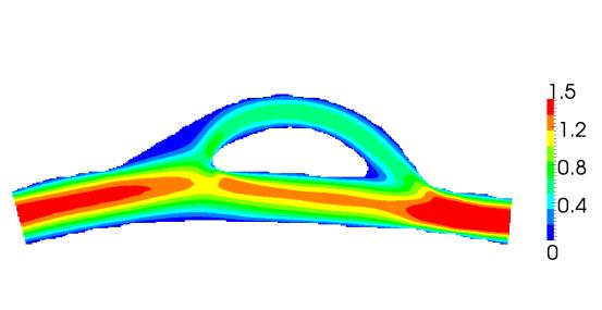
 patient image data of descending aorta, (center) level set field generated from image segmentation")

63 Figure 20: Image to flow simulation on patient specific data. (left) patient image data of descending aorta, (center) level set field generated from image segmentation with interior boundary cap locations marked, (right) velocity magnitude contours at Re of 115 with parabolic inlet velocity profile. Figure 21: Image-to-flow on computer drawn image. (left) 128 x 128 pixel image, (right) Velocity magnitude contours at Re =

 Velocity magnitude")

64 Figure 22: Image-to-flow via scanner. (left) hand drawn image, (right) Velocity magnitude contours at Re = 100. Figure 23: Image-to-flow via cellphone camera. (left) hand drawn image, (right) Velocity magnitude contours at Re =
1.2 Numerical Solutions of Flow Problems
 1.2 Numerical Solutions of Flow Problems DIFFERENTIAL EQUATIONS OF MOTION FOR A SIMPLIFIED FLOW PROBLEM Continuity equation for incompressible flow: 0 Momentum (Navier-Stokes) equations for a Newtonian
Driven Cavity Example
 BMAppendixI.qxd 11/14/12 6:55 PM Page I-1 I CFD Driven Cavity Example I.1 Problem One of the classic benchmarks in CFD is the driven cavity problem. Consider steady, incompressible, viscous flow in a square
Investigation of cross flow over a circular cylinder at low Re using the Immersed Boundary Method (IBM)
") Computational Methods and Experimental Measurements XVII 235 Investigation of cross flow over a circular cylinder at low Re using the Immersed Boundary Method (IBM) K. Rehman Department of Mechanical Engineering,
Computational Methods and Experimental Measurements XVII 235 Investigation of cross flow over a circular cylinder at low Re using the Immersed Boundary Method (IBM) K. Rehman Department of Mechanical Engineering,
ENERGY-224 Reservoir Simulation Project Report. Ala Alzayer
 ENERGY-224 Reservoir Simulation Project Report Ala Alzayer Autumn Quarter December 3, 2014 Contents 1 Objective 2 2 Governing Equations 2 3 Methodolgy 3 3.1 BlockMesh.........................................
Stream Function-Vorticity CFD Solver MAE 6263
 Stream Function-Vorticity CFD Solver MAE 66 Charles O Neill April, 00 Abstract A finite difference CFD solver was developed for transient, two-dimensional Cartesian viscous flows. Flow parameters are solved
A massively parallel adaptive sharp interface solver with application to mechanical heart valve simulations
 University of Iowa Iowa Research Online Theses and Dissertations Fall 2012 A massively parallel adaptive sharp interface solver with application to mechanical heart valve simulations John Arnold Mousel
The Immersed Interface Method
 The Immersed Interface Method Numerical Solutions of PDEs Involving Interfaces and Irregular Domains Zhiiin Li Kazufumi Ito North Carolina State University Raleigh, North Carolina Society for Industrial
Application of Finite Volume Method for Structural Analysis
 Application of Finite Volume Method for Structural Analysis Saeed-Reza Sabbagh-Yazdi and Milad Bayatlou Associate Professor, Civil Engineering Department of KNToosi University of Technology, PostGraduate
Strömningslära Fluid Dynamics. Computer laboratories using COMSOL v4.4
 UMEÅ UNIVERSITY Department of Physics Claude Dion Olexii Iukhymenko May 15, 2015 Strömningslära Fluid Dynamics (5FY144) Computer laboratories using COMSOL v4.4!! Report requirements Computer labs must
cuibm A GPU Accelerated Immersed Boundary Method
 cuibm A GPU Accelerated Immersed Boundary Method S. K. Layton, A. Krishnan and L. A. Barba Corresponding author: labarba@bu.edu Department of Mechanical Engineering, Boston University, Boston, MA, 225,
CPM Specifications Document Healthy Vertebral:
 CPM Specifications Document Healthy Vertebral: OSMSC 0078_0000, 0079_0000, 0166_000, 0167_0000 May 1, 2013 Version 1 Open Source Medical Software Corporation 2013 Open Source Medical Software Corporation.
Development of a Maxwell Equation Solver for Application to Two Fluid Plasma Models. C. Aberle, A. Hakim, and U. Shumlak
 Development of a Maxwell Equation Solver for Application to Two Fluid Plasma Models C. Aberle, A. Hakim, and U. Shumlak Aerospace and Astronautics University of Washington, Seattle American Physical Society
Coupling of STAR-CCM+ to Other Theoretical or Numerical Solutions. Milovan Perić
 Coupling of STAR-CCM+ to Other Theoretical or Numerical Solutions Milovan Perić Contents The need to couple STAR-CCM+ with other theoretical or numerical solutions Coupling approaches: surface and volume
Backward facing step Homework. Department of Fluid Mechanics. For Personal Use. Budapest University of Technology and Economics. Budapest, 2010 autumn
 Backward facing step Homework Department of Fluid Mechanics Budapest University of Technology and Economics Budapest, 2010 autumn Updated: October 26, 2010 CONTENTS i Contents 1 Introduction 1 2 The problem
CFD MODELING FOR PNEUMATIC CONVEYING
 CFD MODELING FOR PNEUMATIC CONVEYING Arvind Kumar 1, D.R. Kaushal 2, Navneet Kumar 3 1 Associate Professor YMCAUST, Faridabad 2 Associate Professor, IIT, Delhi 3 Research Scholar IIT, Delhi e-mail: arvindeem@yahoo.co.in
Computational Simulation of the Wind-force on Metal Meshes
 16 th Australasian Fluid Mechanics Conference Crown Plaza, Gold Coast, Australia 2-7 December 2007 Computational Simulation of the Wind-force on Metal Meshes Ahmad Sharifian & David R. Buttsworth Faculty
Shape optimisation using breakthrough technologies
 Shape optimisation using breakthrough technologies Compiled by Mike Slack Ansys Technical Services 2010 ANSYS, Inc. All rights reserved. 1 ANSYS, Inc. Proprietary Introduction Shape optimisation technologies
Finite Volume Discretization on Irregular Voronoi Grids
 Finite Volume Discretization on Irregular Voronoi Grids C.Huettig 1, W. Moore 1 1 Hampton University / National Institute of Aerospace Folie 1 The earth and its terrestrial neighbors NASA Colin Rose, Dorling
Isogeometric Analysis of Fluid-Structure Interaction
 Isogeometric Analysis of Fluid-Structure Interaction Y. Bazilevs, V.M. Calo, T.J.R. Hughes Institute for Computational Engineering and Sciences, The University of Texas at Austin, USA e-mail: {bazily,victor,hughes}@ices.utexas.edu
Edge and local feature detection - 2. Importance of edge detection in computer vision
 Edge and local feature detection Gradient based edge detection Edge detection by function fitting Second derivative edge detectors Edge linking and the construction of the chain graph Edge and local feature
Adarsh Krishnamurthy (cs184-bb) Bela Stepanova (cs184-bs)
 Bela Stepanova (cs184-bs)") OBJECTIVE FLUID SIMULATIONS Adarsh Krishnamurthy (cs184-bb) Bela Stepanova (cs184-bs) The basic objective of the project is the implementation of the paper Stable Fluids (Jos Stam, SIGGRAPH 99). The final
OBJECTIVE FLUID SIMULATIONS Adarsh Krishnamurthy (cs184-bb) Bela Stepanova (cs184-bs) The basic objective of the project is the implementation of the paper Stable Fluids (Jos Stam, SIGGRAPH 99). The final
FAST ALGORITHMS FOR CALCULATIONS OF VISCOUS INCOMPRESSIBLE FLOWS USING THE ARTIFICIAL COMPRESSIBILITY METHOD
 TASK QUARTERLY 12 No 3, 273 287 FAST ALGORITHMS FOR CALCULATIONS OF VISCOUS INCOMPRESSIBLE FLOWS USING THE ARTIFICIAL COMPRESSIBILITY METHOD ZBIGNIEW KOSMA Institute of Applied Mechanics, Technical University
Simulation of Flow Development in a Pipe
 Tutorial 4. Simulation of Flow Development in a Pipe Introduction The purpose of this tutorial is to illustrate the setup and solution of a 3D turbulent fluid flow in a pipe. The pipe networks are common
Using a Single Rotating Reference Frame
 Tutorial 9. Using a Single Rotating Reference Frame Introduction This tutorial considers the flow within a 2D, axisymmetric, co-rotating disk cavity system. Understanding the behavior of such flows is
11/1/13. Visualization. Scientific Visualization. Types of Data. Height Field. Contour Curves. Meshes
 CSCI 420 Computer Graphics Lecture 26 Visualization Height Fields and Contours Scalar Fields Volume Rendering Vector Fields [Angel Ch. 2.11] Jernej Barbic University of Southern California Scientific Visualization
Visualization. CSCI 420 Computer Graphics Lecture 26
 CSCI 420 Computer Graphics Lecture 26 Visualization Height Fields and Contours Scalar Fields Volume Rendering Vector Fields [Angel Ch. 11] Jernej Barbic University of Southern California 1 Scientific Visualization
ALE Seamless Immersed Boundary Method with Overset Grid System for Multiple Moving Objects
 Tenth International Conference on Computational Fluid Dynamics (ICCFD10), Barcelona,Spain, July 9-13, 2018 ICCFD10-047 ALE Seamless Immersed Boundary Method with Overset Grid System for Multiple Moving
Partial Differential Equations
 Simulation in Computer Graphics Partial Differential Equations Matthias Teschner Computer Science Department University of Freiburg Motivation various dynamic effects and physical processes are described
Manipulating the Boundary Mesh
 Chapter 7. Manipulating the Boundary Mesh The first step in producing an unstructured grid is to define the shape of the domain boundaries. Using a preprocessor (GAMBIT or a third-party CAD package) you
Introduction to ANSYS CFX
 Workshop 03 Fluid flow around the NACA0012 Airfoil 16.0 Release Introduction to ANSYS CFX 2015 ANSYS, Inc. March 13, 2015 1 Release 16.0 Workshop Description: The flow simulated is an external aerodynamics
NUMERICAL VISCOSITY. Convergent Science White Paper. COPYRIGHT 2017 CONVERGENT SCIENCE. All rights reserved.
 Convergent Science White Paper COPYRIGHT 2017 CONVERGENT SCIENCE. All rights reserved. This document contains information that is proprietary to Convergent Science. Public dissemination of this document
MESHLESS SOLUTION OF INCOMPRESSIBLE FLOW OVER BACKWARD-FACING STEP
 Vol. 12, Issue 1/2016, 63-68 DOI: 10.1515/cee-2016-0009 MESHLESS SOLUTION OF INCOMPRESSIBLE FLOW OVER BACKWARD-FACING STEP Juraj MUŽÍK 1,* 1 Department of Geotechnics, Faculty of Civil Engineering, University
Tutorial School on Fluid Dynamics: Topics in Turbulence May 24-28, 2010
 Applications of Large-eddy Simulation to Biological Flows Tutorial School on Fluid Dynamics: Topics in Turbulence May 24-28, 2010 Methodologies & Applications Elias Balaras Fischell Department of Bioengineering
µ = Pa s m 3 The Reynolds number based on hydraulic diameter, D h = 2W h/(w + h) = 3.2 mm for the main inlet duct is = 359
 = 3.2 mm for the main inlet duct is = 359") Laminar Mixer Tutorial for STAR-CCM+ ME 448/548 March 30, 2014 Gerald Recktenwald gerry@pdx.edu 1 Overview Imagine that you are part of a team developing a medical diagnostic device. The device has a millimeter
Laminar Mixer Tutorial for STAR-CCM+ ME 448/548 March 30, 2014 Gerald Recktenwald gerry@pdx.edu 1 Overview Imagine that you are part of a team developing a medical diagnostic device. The device has a millimeter
Life Sciences Applications: Modeling and Simulation for Biomedical Device Design SGC 2013
 Life Sciences Applications: Modeling and Simulation for Biomedical Device Design Kristian.Debus@cd-adapco.com SGC 2013 Modeling and Simulation for Biomedical Device Design Biomedical device design and
FEMLAB Exercise 1 for ChE366
 FEMLAB Exercise 1 for ChE366 Problem statement Consider a spherical particle of radius r s moving with constant velocity U in an infinitely long cylinder of radius R that contains a Newtonian fluid. Let
Commercial Implementations of Optimization Software and its Application to Fluid Dynamics Problems
 Commercial Implementations of Optimization Software and its Application to Fluid Dynamics Problems Szymon Buhajczuk, M.A.Sc SimuTech Group Toronto Fields Institute Optimization Seminar December 6, 2011
Introduction to ANSYS ICEM CFD
 Lecture 4 Volume Meshing 14. 0 Release Introduction to ANSYS ICEM CFD 1 2011 ANSYS, Inc. March 21, 2012 Introduction to Volume Meshing To automatically create 3D elements to fill volumetric domain Generally
Preliminary Spray Cooling Simulations Using a Full-Cone Water Spray
 39th Dayton-Cincinnati Aerospace Sciences Symposium Preliminary Spray Cooling Simulations Using a Full-Cone Water Spray Murat Dinc Prof. Donald D. Gray (advisor), Prof. John M. Kuhlman, Nicholas L. Hillen,
Surface Reconstruction. Gianpaolo Palma
 Surface Reconstruction Gianpaolo Palma Surface reconstruction Input Point cloud With or without normals Examples: multi-view stereo, union of range scan vertices Range scans Each scan is a triangular mesh
Visualization. Images are used to aid in understanding of data. Height Fields and Contours Scalar Fields Volume Rendering Vector Fields [chapter 26]
![Visualization. Images are used to aid in understanding of data. Height Fields and Contours Scalar Fields Volume Rendering Vector Fields [chapter 26]](/thumbs/74/70771954.jpg "Visualization. Images are used to aid in understanding of data. Height Fields and Contours Scalar Fields Volume Rendering Vector Fields [chapter 26]") Visualization Images are used to aid in understanding of data Height Fields and Contours Scalar Fields Volume Rendering Vector Fields [chapter 26] Tumor SCI, Utah Scientific Visualization Visualize large
Visualization Images are used to aid in understanding of data Height Fields and Contours Scalar Fields Volume Rendering Vector Fields [chapter 26] Tumor SCI, Utah Scientific Visualization Visualize large
CSE 554 Lecture 6: Fairing and Simplification
 CSE 554 Lecture 6: Fairing and Simplification Fall 2012 CSE554 Fairing and simplification Slide 1 Review Iso-contours in grayscale images and volumes Piece-wise linear representations Polylines (2D) and
Supersonic Flow Over a Wedge
 SPC 407 Supersonic & Hypersonic Fluid Dynamics Ansys Fluent Tutorial 2 Supersonic Flow Over a Wedge Ahmed M Nagib Elmekawy, PhD, P.E. Problem Specification A uniform supersonic stream encounters a wedge
FLUENT Secondary flow in a teacup Author: John M. Cimbala, Penn State University Latest revision: 26 January 2016
 FLUENT Secondary flow in a teacup Author: John M. Cimbala, Penn State University Latest revision: 26 January 2016 Note: These instructions are based on an older version of FLUENT, and some of the instructions
coding of various parts showing different features, the possibility of rotation or of hiding covering parts of the object's surface to gain an insight
 Three-Dimensional Object Reconstruction from Layered Spatial Data Michael Dangl and Robert Sablatnig Vienna University of Technology, Institute of Computer Aided Automation, Pattern Recognition and Image
Tutorial 2. Modeling Periodic Flow and Heat Transfer
 Tutorial 2. Modeling Periodic Flow and Heat Transfer Introduction: Many industrial applications, such as steam generation in a boiler or air cooling in the coil of an air conditioner, can be modeled as
CFD simulations of blood flow through abdominal part of aorta
 CFD simulations of blood flow through abdominal part of aorta Andrzej Polanczyk, Aleksandra Piechota Faculty of Process and Enviromental Engineering, Technical University of Lodz, Wolczanska 13 90-94 Lodz,
2.7 Cloth Animation. Jacobs University Visualization and Computer Graphics Lab : Advanced Graphics - Chapter 2 123
 2.7 Cloth Animation 320491: Advanced Graphics - Chapter 2 123 Example: Cloth draping Image Michael Kass 320491: Advanced Graphics - Chapter 2 124 Cloth using mass-spring model Network of masses and springs
Visualization Computer Graphics I Lecture 20
 15-462 Computer Graphics I Lecture 20 Visualization Height Fields and Contours Scalar Fields Volume Rendering Vector Fields [Angel Ch. 12] April 15, 2003 Frank Pfenning Carnegie Mellon University http://www.cs.cmu.edu/~fp/courses/graphics/
Using the Discrete Ordinates Radiation Model
 Tutorial 6. Using the Discrete Ordinates Radiation Model Introduction This tutorial illustrates the set up and solution of flow and thermal modelling of a headlamp. The discrete ordinates (DO) radiation
Height Fields and Contours Scalar Fields Volume Rendering Vector Fields [Angel Ch. 12] April 23, 2002 Frank Pfenning Carnegie Mellon University
![Height Fields and Contours Scalar Fields Volume Rendering Vector Fields [Angel Ch. 12] April 23, 2002 Frank Pfenning Carnegie Mellon University](/thumbs/90/102611276.jpg "Height Fields and Contours Scalar Fields Volume Rendering Vector Fields [Angel Ch. 12] April 23, 2002 Frank Pfenning Carnegie Mellon University") 15-462 Computer Graphics I Lecture 21 Visualization Height Fields and Contours Scalar Fields Volume Rendering Vector Fields [Angel Ch. 12] April 23, 2002 Frank Pfenning Carnegie Mellon University http://www.cs.cmu.edu/~fp/courses/graphics/
15-462 Computer Graphics I Lecture 21 Visualization Height Fields and Contours Scalar Fields Volume Rendering Vector Fields [Angel Ch. 12] April 23, 2002 Frank Pfenning Carnegie Mellon University http://www.cs.cmu.edu/~fp/courses/graphics/
Application of Wray-Agarwal Turbulence Model for Accurate Numerical Simulation of Flow Past a Three-Dimensional Wing-body
 Washington University in St. Louis Washington University Open Scholarship Mechanical Engineering and Materials Science Independent Study Mechanical Engineering & Materials Science 4-28-2016 Application
The goal is the definition of points with numbers and primitives with equations or functions. The definition of points with numbers requires a
 The goal is the definition of points with numbers and primitives with equations or functions. The definition of points with numbers requires a coordinate system and then the measuring of the point with
NUMERICAL 3D TRANSONIC FLOW SIMULATION OVER A WING
 Review of the Air Force Academy No.3 (35)/2017 NUMERICAL 3D TRANSONIC FLOW SIMULATION OVER A WING Cvetelina VELKOVA Department of Technical Mechanics, Naval Academy Nikola Vaptsarov,Varna, Bulgaria (cvetelina.velkova1985@gmail.com)
Introduction to C omputational F luid Dynamics. D. Murrin
 Introduction to C omputational F luid Dynamics D. Murrin Computational fluid dynamics (CFD) is the science of predicting fluid flow, heat transfer, mass transfer, chemical reactions, and related phenomena
Visualization Computer Graphics I Lecture 20
 15-462 Computer Graphics I Lecture 20 Visualization Height Fields and Contours Scalar Fields Volume Rendering Vector Fields [Angel Ch. 12] November 20, 2003 Doug James Carnegie Mellon University http://www.cs.cmu.edu/~djames/15-462/fall03
Mid-Year Report. Discontinuous Galerkin Euler Equation Solver. Friday, December 14, Andrey Andreyev. Advisor: Dr.
 Mid-Year Report Discontinuous Galerkin Euler Equation Solver Friday, December 14, 2012 Andrey Andreyev Advisor: Dr. James Baeder Abstract: The focus of this effort is to produce a two dimensional inviscid,
Optimizing Bio-Inspired Flow Channel Design on Bipolar Plates of PEM Fuel Cells
 Excerpt from the Proceedings of the COMSOL Conference 2010 Boston Optimizing Bio-Inspired Flow Channel Design on Bipolar Plates of PEM Fuel Cells James A. Peitzmeier *1, Steven Kapturowski 2 and Xia Wang
Overview of Traditional Surface Tracking Methods
 Liquid Simulation With Mesh-Based Surface Tracking Overview of Traditional Surface Tracking Methods Matthias Müller Introduction Research lead of NVIDIA PhysX team PhysX GPU acc. Game physics engine www.nvidia.com\physx
Simulation of Turbulent Flow around an Airfoil
 1. Purpose Simulation of Turbulent Flow around an Airfoil ENGR:2510 Mechanics of Fluids and Transfer Processes CFD Lab 2 (ANSYS 17.1; Last Updated: Nov. 7, 2016) By Timur Dogan, Michael Conger, Andrew
SUPPLEMENTARY FILE S1: 3D AIRWAY TUBE RECONSTRUCTION AND CELL-BASED MECHANICAL MODEL. RELATED TO FIGURE 1, FIGURE 7, AND STAR METHODS.
 SUPPLEMENTARY FILE S1: 3D AIRWAY TUBE RECONSTRUCTION AND CELL-BASED MECHANICAL MODEL. RELATED TO FIGURE 1, FIGURE 7, AND STAR METHODS. 1. 3D AIRWAY TUBE RECONSTRUCTION. RELATED TO FIGURE 1 AND STAR METHODS
CFD Post-Processing of Rampressor Rotor Compressor
 Gas Turbine Industrial Fellowship Program 2006 CFD Post-Processing of Rampressor Rotor Compressor Curtis Memory, Brigham Young niversity Ramgen Power Systems Mentor: Rob Steele I. Introduction Recent movements
STAR-CCM+: Wind loading on buildings SPRING 2018
 STAR-CCM+: Wind loading on buildings SPRING 2018 1. Notes on the software 2. Assigned exercise (submission via Blackboard; deadline: Thursday Week 3, 11 pm) 1. NOTES ON THE SOFTWARE STAR-CCM+ generates
Introduction to Computational Fluid Dynamics Mech 122 D. Fabris, K. Lynch, D. Rich
 Introduction to Computational Fluid Dynamics Mech 122 D. Fabris, K. Lynch, D. Rich 1 Computational Fluid dynamics Computational fluid dynamics (CFD) is the analysis of systems involving fluid flow, heat
FOURTH ORDER COMPACT FORMULATION OF STEADY NAVIER-STOKES EQUATIONS ON NON-UNIFORM GRIDS
 International Journal of Mechanical Engineering and Technology (IJMET Volume 9 Issue 10 October 2018 pp. 179 189 Article ID: IJMET_09_10_11 Available online at http://www.iaeme.com/ijmet/issues.asp?jtypeijmet&vtype9&itype10
Moving Interface Problems: Methods & Applications Tutorial Lecture II
 Moving Interface Problems: Methods & Applications Tutorial Lecture II Grétar Tryggvason Worcester Polytechnic Institute Moving Interface Problems and Applications in Fluid Dynamics Singapore National University,
Verification and Validation of Turbulent Flow around a Clark-Y Airfoil
 1 Verification and Validation of Turbulent Flow around a Clark-Y Airfoil 1. Purpose ME:5160 Intermediate Mechanics of Fluids CFD LAB 2 (ANSYS 19.1; Last Updated: Aug. 7, 2018) By Timur Dogan, Michael Conger,
Guidelines for proper use of Plate elements
 Guidelines for proper use of Plate elements In structural analysis using finite element method, the analysis model is created by dividing the entire structure into finite elements. This procedure is known
Level set methods Formulation of Interface Propagation Boundary Value PDE Initial Value PDE Motion in an externally generated velocity field
 Level Set Methods Overview Level set methods Formulation of Interface Propagation Boundary Value PDE Initial Value PDE Motion in an externally generated velocity field Convection Upwind ddifferencingi
CS205b/CME306. Lecture 9
 CS205b/CME306 Lecture 9 1 Convection Supplementary Reading: Osher and Fedkiw, Sections 3.3 and 3.5; Leveque, Sections 6.7, 8.3, 10.2, 10.4. For a reference on Newton polynomial interpolation via divided
Introduction to Computer Graphics. Modeling (3) April 27, 2017 Kenshi Takayama
 April 27, 2017 Kenshi Takayama") Introduction to Computer Graphics Modeling (3) April 27, 2017 Kenshi Takayama Solid modeling 2 Solid models Thin shapes represented by single polygons Unorientable Clear definition of inside & outside
Introduction to Computer Graphics Modeling (3) April 27, 2017 Kenshi Takayama Solid modeling 2 Solid models Thin shapes represented by single polygons Unorientable Clear definition of inside & outside
Problem description. The FCBI-C element is used in the fluid part of the model.
 Problem description This tutorial illustrates the use of ADINA for analyzing the fluid-structure interaction (FSI) behavior of a flexible splitter behind a 2D cylinder and the surrounding fluid in a channel.
Chapter 24. Creating Surfaces for Displaying and Reporting Data
 Chapter 24. Creating Surfaces for Displaying and Reporting Data FLUENT allows you to select portions of the domain to be used for visualizing the flow field. The domain portions are called surfaces, and
A Verification Study of ABAQUS AC3D8R Elements for Acoustic Wave Propagation
 A Verification Study of ABAQUS AC3D8R Elements for Acoustic Wave Propagation by Michael Robert Hubenthal A Project Submitted to the Graduate Faculty of Rensselaer Polytechnic Institute in Partial Fulfillment
and to the following students who assisted in the creation of the Fluid Dynamics tutorials:
 Fluid Dynamics CAx Tutorial: Channel Flow Basic Tutorial # 4 Deryl O. Snyder C. Greg Jensen Brigham Young University Provo, UT 84602 Special thanks to: PACE, Fluent, UGS Solutions, Altair Engineering;
Volume visualization. Volume visualization. Volume visualization methods. Sources of volume visualization. Sources of volume visualization
 Volume visualization Volume visualization Volumes are special cases of scalar data: regular 3D grids of scalars, typically interpreted as density values. Each data value is assumed to describe a cubic
Module D: Laminar Flow over a Flat Plate
 Module D: Laminar Flow over a Flat Plate Summary... Problem Statement Geometry and Mesh Creation Problem Setup Solution. Results Validation......... Mesh Refinement.. Summary This ANSYS FLUENT tutorial
Flow and Heat Transfer in a Mixing Elbow
 Flow and Heat Transfer in a Mixing Elbow Objectives The main objectives of the project are to learn (i) how to set up and perform flow simulations with heat transfer and mixing, (ii) post-processing and
ISSN(PRINT): ,(ONLINE): ,VOLUME-1,ISSUE-1,
: ,(ONLINE): ,VOLUME-1,ISSUE-1,") NUMERICAL ANALYSIS OF THE TUBE BANK PRESSURE DROP OF A SHELL AND TUBE HEAT EXCHANGER Kartik Ajugia, Kunal Bhavsar Lecturer, Mechanical Department, SJCET Mumbai University, Maharashtra Assistant Professor,
NUMERICAL ANALYSIS OF THE TUBE BANK PRESSURE DROP OF A SHELL AND TUBE HEAT EXCHANGER Kartik Ajugia, Kunal Bhavsar Lecturer, Mechanical Department, SJCET Mumbai University, Maharashtra Assistant Professor,
Modeling Unsteady Compressible Flow
 Tutorial 4. Modeling Unsteady Compressible Flow Introduction In this tutorial, FLUENT s density-based implicit solver is used to predict the timedependent flow through a two-dimensional nozzle. As an initial
STABILIZED FINITE ELEMENT METHODS FOR INCOMPRESSIBLE FLOWS WITH EMPHASIS ON MOVING BOUNDARIES AND INTERFACES
 STABILIZED FINITE ELEMENT METHODS FOR INCOMPRESSIBLE FLOWS WITH EMPHASIS ON MOVING BOUNDARIES AND INTERFACES A THESIS SUBMITTED TO THE FACULTY OF THE GRADUATE SCHOOL OF THE UNIVERSITY OF MINNESOTA BY Marek
Debojyoti Ghosh. Adviser: Dr. James Baeder Alfred Gessow Rotorcraft Center Department of Aerospace Engineering
 Debojyoti Ghosh Adviser: Dr. James Baeder Alfred Gessow Rotorcraft Center Department of Aerospace Engineering To study the Dynamic Stalling of rotor blade cross-sections Unsteady Aerodynamics: Time varying
COMPUTATIONAL FLUID DYNAMICS ANALYSIS OF ORIFICE PLATE METERING SITUATIONS UNDER ABNORMAL CONFIGURATIONS
 COMPUTATIONAL FLUID DYNAMICS ANALYSIS OF ORIFICE PLATE METERING SITUATIONS UNDER ABNORMAL CONFIGURATIONS Dr W. Malalasekera Version 3.0 August 2013 1 COMPUTATIONAL FLUID DYNAMICS ANALYSIS OF ORIFICE PLATE
Auto Injector Syringe. A Fluent Dynamic Mesh 1DOF Tutorial
 Auto Injector Syringe A Fluent Dynamic Mesh 1DOF Tutorial 1 2015 ANSYS, Inc. June 26, 2015 Prerequisites This tutorial is written with the assumption that You have attended the Introduction to ANSYS Fluent
Discrete representations of geometric objects: Features, data structures and adequacy for dynamic simulation. Part I : Solid geometry
 Discrete representations of geometric objects: Features, data structures and adequacy for dynamic simulation. Surfaces Part I : Solid geometry hachar Fleishman Tel Aviv University David Levin Claudio T.
Accurate and Efficient Turbomachinery Simulation. Chad Custer, PhD Turbomachinery Technical Specialist
 Accurate and Efficient Turbomachinery Simulation Chad Custer, PhD Turbomachinery Technical Specialist Outline Turbomachinery simulation advantages Axial fan optimization Description of design objectives
Lab 9: FLUENT: Transient Natural Convection Between Concentric Cylinders
 Lab 9: FLUENT: Transient Natural Convection Between Concentric Cylinders Objective: The objective of this laboratory is to introduce how to use FLUENT to solve both transient and natural convection problems.
Simulation of Turbulent Flow around an Airfoil
 Simulation of Turbulent Flow around an Airfoil ENGR:2510 Mechanics of Fluids and Transfer Processes CFD Pre-Lab 2 (ANSYS 17.1; Last Updated: Nov. 7, 2016) By Timur Dogan, Michael Conger, Andrew Opyd, Dong-Hwan
CS 231. Fluid simulation
 CS 231 Fluid simulation Why Simulate Fluids? Feature film special effects Computer games Medicine (e.g. blood flow in heart) Because it s fun Fluid Simulation Called Computational Fluid Dynamics (CFD)
Tutorial 1. Introduction to Using FLUENT: Fluid Flow and Heat Transfer in a Mixing Elbow
 Tutorial 1. Introduction to Using FLUENT: Fluid Flow and Heat Transfer in a Mixing Elbow Introduction This tutorial illustrates the setup and solution of the two-dimensional turbulent fluid flow and heat
Fluent User Services Center
 Solver Settings 5-1 Using the Solver Setting Solver Parameters Convergence Definition Monitoring Stability Accelerating Convergence Accuracy Grid Independence Adaption Appendix: Background Finite Volume
Computation of Velocity, Pressure and Temperature Distributions near a Stagnation Point in Planar Laminar Viscous Incompressible Flow
 Excerpt from the Proceedings of the COMSOL Conference 8 Boston Computation of Velocity, Pressure and Temperature Distributions near a Stagnation Point in Planar Laminar Viscous Incompressible Flow E. Kaufman
Verification of Laminar and Validation of Turbulent Pipe Flows
 1 Verification of Laminar and Validation of Turbulent Pipe Flows 1. Purpose ME:5160 Intermediate Mechanics of Fluids CFD LAB 1 (ANSYS 18.1; Last Updated: Aug. 1, 2017) By Timur Dogan, Michael Conger, Dong-Hwan
Computer Project 3. AA Computational Fluid Dyanmics University of Washington. Mishaal Aleem March 17, 2015
 Computer Project 3 AA 543 - Computational Fluid Dyanmics University of Washington Mishaal Aleem March 17, 2015 Contents Introduction........................................... 1 3.1 Grid Generator.......................................
Unstructured Mesh Generation for Implicit Moving Geometries and Level Set Applications
 Unstructured Mesh Generation for Implicit Moving Geometries and Level Set Applications Per-Olof Persson (persson@mit.edu) Department of Mathematics Massachusetts Institute of Technology http://www.mit.edu/
COMPUTATIONAL FLUID DYNAMICS USED IN THE DESIGN OF WATERBLAST TOOLING
 2015 WJTA-IMCA Conference and Expo November 2-4 New Orleans, Louisiana Paper COMPUTATIONAL FLUID DYNAMICS USED IN THE DESIGN OF WATERBLAST TOOLING J. Schneider StoneAge, Inc. Durango, Colorado, U.S.A.
CFD Analysis of a Fully Developed Turbulent Flow in a Pipe with a Constriction and an Obstacle
 CFD Analysis of a Fully Developed Turbulent Flow in a Pipe with a Constriction and an Obstacle C, Diyoke Mechanical Engineering Department Enugu State University of Science & Tech. Enugu, Nigeria U, Ngwaka
Sweeping Jet Flushing Method for EDM
 International Conference on Multidisciplinary Research & Practice P a g e 192 Sweeping Jet Flushing Method for EDM Kishor K Kulkarni # Production Engineering, ShivajiUniversity/Ashokrao Mane Group of Institution
Revised Sheet Metal Simulation, J.E. Akin, Rice University
 Revised Sheet Metal Simulation, J.E. Akin, Rice University A SolidWorks simulation tutorial is just intended to illustrate where to find various icons that you would need in a real engineering analysis.
Overview and Recent Developments of Dynamic Mesh Capabilities
 Overview and Recent Developments of Dynamic Mesh Capabilities Henrik Rusche and Hrvoje Jasak h.rusche@wikki-gmbh.de and h.jasak@wikki.co.uk Wikki Gmbh, Germany Wikki Ltd, United Kingdom 6th OpenFOAM Workshop,