L E A R N I N G O B JE C T I V E S

Transcription

1 2.2 Measures of Central Location L E A R N I N G O B JE C T I V E S 1. To learn the concept of the center of a data set. 2. To learn the meaning of each of three measures of the center of a data set the mean, the median, and the mode and how to compute each one. This section could be titled three kinds of averages of a data set. Any kind of average is meant to be an answer to the question Where do the data center? It is thus a measure of the central location of the data set. We will see that the nature of the data set, as indicated by a relative frequency histogram, will determine what constitutes a good answer. Different shapes of the histogram call for different measures of central location. 29

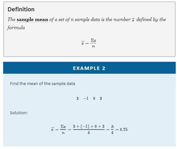
2 The Mean The first measure of central location is the usual average that is familiar to everyone. In the formula in the following definition we introduce the standard summation notation Σ, where Σ is the capital Greek letter sigma. In general, the notation Σ followed by a second mathematical symbol means to add up all the values that the second symbol can take in the context of the problem. Here is an example to illustrate this. In the definition we follow the convention of using lowercase n to denote the number of measurements in a sample, which is called the sample size. 30

3 31

4 32

5 33

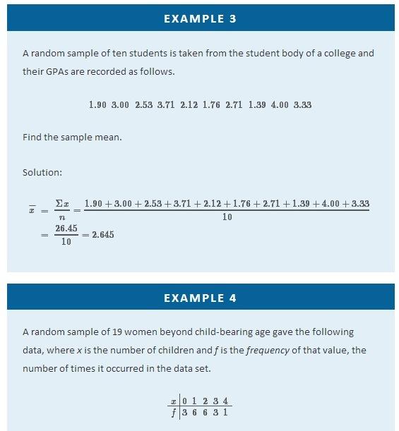
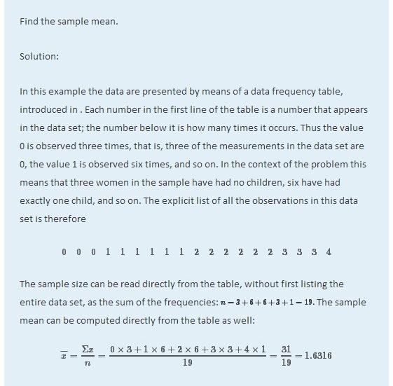
6 In the examples above the data sets were described as samples. Therefore the means were sample means, denoted by x. If the data come from a census, so that there is a measurement for every element of the population, then the mean is calculated by exactly the same process of summing all the measurements and dividing by how many of them there are, but it is now the population mean and is denoted by μ, the lower case Greek letter mu. The mean of two numbers is the number that is halfway between them. For example, the average of the numbers 5 and 17 is (5 + 17) 2 = 11, which is 6 units above 5 and 6 units below 17. In this sense the average 11 is the center of the data set {5,17}. For larger data sets the mean can similarly be regarded as the center of the data. The Median To see why another concept of average is needed, consider the following situation. Suppose we are interested in the average yearly income of employees at a large corporation. We take a random sample of seven employees, obtaining the sample data (rounded to the nearest hundred dollars, and expressed in thousands of dollars) The mean (rounded to one decimal place) is x -47.4, but the statement the average income of employees at this corporation is $47,400 is surely misleading. It is approximately twice what six of the seven employees in the sample make and is nowhere near what any of them makes. It is easy to see what went wrong: the presence of the one executive in the sample, whose salary is so large compared to everyone else s, caused the numerator in the formula for the sample mean to be far too large, pulling the mean far to the right of where we think that the average ought to be, namely around $24,000 or $25,000. The number in our data set is called an outlier, a number that is far removed from most or all of the remaining measurements. Many times an outlier is the result of some sort of error, but not always, as is 34

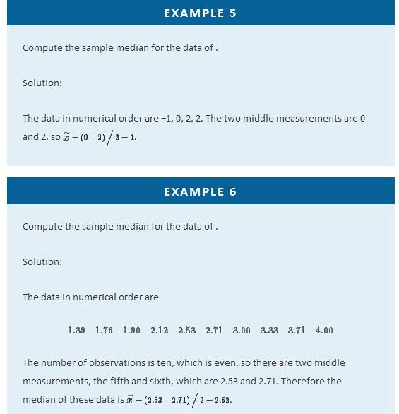
7 the case here. We would get a better measure of the center of the data if we were to arrange the data in numerical order, then select the middle number in the list, in this case The result is called the median of the data set, and has the property that roughly half of the measurements are larger than it is, and roughly half are smaller. In this sense it locates the center of the data. If there are an even number of measurements in the data set, then there will be two middle elements when all are lined up in order, so we take the mean of the middle two as the median. Thus we have the following definition. Definition The sample median x^~ of a set of sample data for which there are an odd number of measurements is the middle measurement when the data are arranged in numerical order. The sample median x^~ of a set of sample data for which there are an even number of measurements is the mean of the two middle measurements when the data are arranged in numerical order. The population median is defined in a similar way, but we will not have occasion to refer to it again in this text. The median is a value that divides the observations in a data set so that 50% of the data are on its left and the other 50% on its right. In accordance with, therefore, in the curve that represents the distribution of the data, a vertical line drawn at the median divides the area in two, area 0.5 (50% of the total area 1) to the left and area 0.5 (50% of the total area 1) to the right, as shown in. In our income example themedian, $24,600, clearly gave a much better measure of the middle of the data set than did the mean $47,400. This is typical for situations in which the distribution is skewed. (Skewness and symmetry of distributions are discussed at the end of this subsection.) 35

8 Figure 2.7 The Median 36

9 37

10 The relationship between the mean and the median for several common shapes of distributions is shown in. The distributions in panels (a) and (b) are said to be symmetric because of the symmetry that they exhibit. The distributions in the remaining two panels are said to be skewed. In each distribution we have drawn a vertical line that divides the area under the curve in half, which in accordance with is located at the median. The following facts are true in general: a. When the distribution is symmetric, as in panels (a) and (b) of, the mean and the median are equal. 38

11 b. When the distribution is as shown in panel (c) of, it is said to be skewed right. The mean has been pulled to the right of the median by the long right tail of the distribution, the few relatively large data values. c. When the distribution is as shown in panel (d) of, it is said to be skewed left. The mean has been pulled to the left of the median by the long left tail of the distribution, the few relatively small data values. Figure 2.8 Skewness of Relative Frequency Histograms The Mode Perhaps you have heard a statement like The average number of automobiles owned by households in the United States is 1.37, and have been amused at the thought of a fraction of an automobile 39

12 sitting in a driveway. In such a context the following measure for central location might make more sense. Definition The sample mode of a set of sample data is the most frequently occurring value. The population mode is defined in a similar way, but we will not have occasion to refer to it again in this text. On a relative frequency histogram, the highest point of the histogram corresponds to the mode of the data set. illustrates the mode. Figure 2.9 Mode For any data set there is always exactly one mean and exactly one median. This need not be true of the mode; several different values could occur with the highest frequency, as we will see. It could even happen 40

13 that every value occurs with the same frequency, in which case the concept of the mode does not make much sense. E X A M P L E 8 Find the mode of the following data set Solution: The value 0 is most frequently observed and therefore the mode is 0. E X A M P L E 9 Compute the sample mode for the data of. Solution: The two most frequently observed values in the data set are 1 and 2. Therefore mode is a set of two values: {1,2}. The mode is a measure of central location since most real-life data sets have moreobservations near the center of the data range and fewer observations on the lower and upper ends. The value with the highest frequency is often in the middle of the data range. K E Y T A K E A W A Y The mean, the median, and the mode each answer the question Where is the center of the data set? The nature of the data set, as indicated by a relative frequency histogram, determines which one gives the best answer. 41

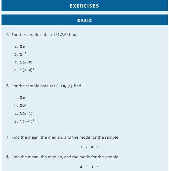
14 42

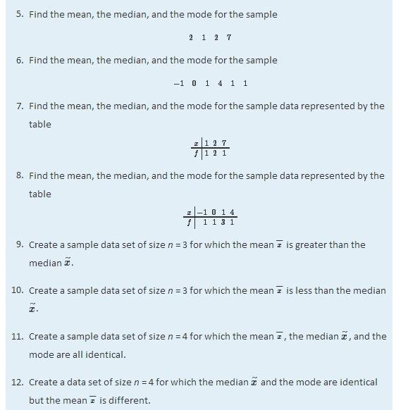
15 43

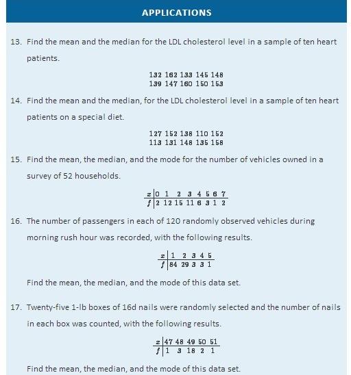
16 44

17 45

18 46

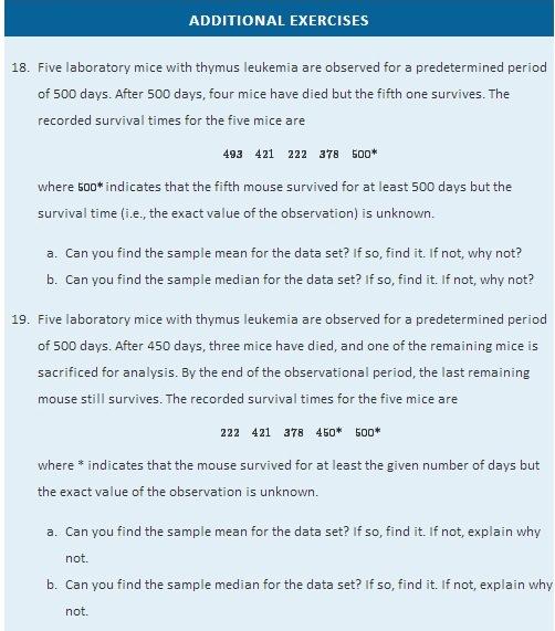
19 47

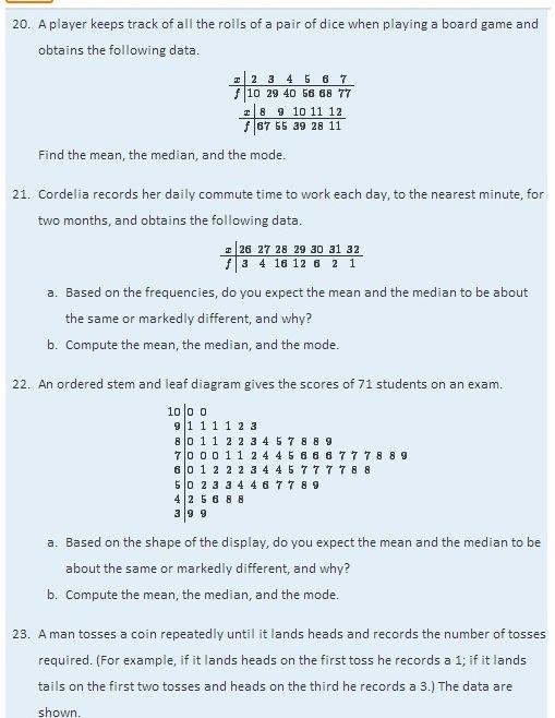
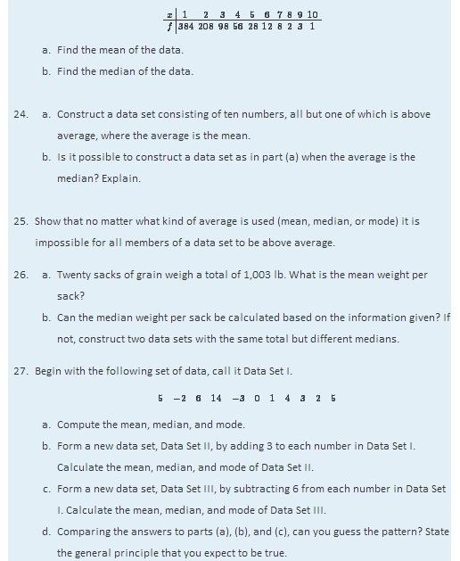
20 L A R G E D A T A S E T E X E R C I S E S 28. Large Data Set 1 lists the SAT scores and GPAs of 1,000 students. a. Compute the mean and median of the 1,000 SAT scores. b. Compute the mean and median of the 1,000 GPAs. 29. Large Data Set 1 lists the SAT scores of 1,000 students. a. Regard the data as arising from a census of all students at a high school, in which the SAT score of every student was measured. Compute the population mean μ. b. Regard the first 25 observations as a random sample drawn from this population. Compute the sample mean x^ and compare it to μ. c. Regard the next 25 observations as a random sample drawn from this population. Compute the sample mean x^ and compare it to μ. 30. Large Data Set 1 lists the GPAs of 1,000 students. a. Regard the data as arising from a census of all freshman at a small college at the end of their first academic year of college study, in which the GPA of every such person was measured. Compute the population mean μ. b. Regard the first 25 observations as a random sample drawn from this population. Compute the sample mean x^ and compare it to μ. c. Regard the next 25 observations as a random sample drawn from this population. Compute the sample mean x^ and compare it to μ. 31. Large Data Sets 7, 7A, and 7B list the survival times in days of 140 laboratory mice with thymic leukemia from onset to death a. Compute the mean and median survival time for all mice, without regard to gender. b. Compute the mean and median survival time for the 65 male mice (separately recorded in Large Data Set 7A). c. Compute the mean and median survival time for the 75 female mice (separately recorded in Large Data Set 7B). 48

21 49

22 2.3 Measures of Variability L E A R N I N G O B JE C T I V E S 1. To learn the concept of the variability of a data set. 2. To learn how to compute three measures of the variability of a data set: the range, the variance, and the standard deviation. Look at the two data sets in Table 2.1 "Two Data Sets" and the graphical representation of each, called a dot plot, in Figure 2.10 "Dot Plots of Data Sets". Table 2.1 Two Data Sets Data Set I: Data Set II: