FAsT-Match: Fast Affine Template Matching

Transcription

1 International Journal on Computer ision manuscript No. (will be inserted by the editor) FAsT-Match: Fast Affine Template Matching Simon Korman Daniel Reichman Gilad Tsur Shai Avidan Received: date / Accepted: date Abstract Fast-Match is a fast algorithm for approximate template matching under 2D affine transformations that minimizes the Sum-of-Absolute-Differences (SAD) error measure. There is a huge number of transformations to consider but we prove that they can be sampled using a density that depends on the smoothness of the image. For each potential transformation, we approximate the SAD error using a sublinear algorithm that randomly examines only a small number of pixels. We further accelerate the algorithm using a branch-and-bound scheme. As images are known to be piecewise smooth, the result is a practical affine template matching algorithm with approximation guarantees, that takes a few seconds to run on a standard machine. We perform several experiments on three different datasets, and report very good results. Keywords Pattern matching template matching image matching sublinear algorithms This work was supported by the Israel Science Foundation (grant No. 873/08, in part) and the Ministry of Science and Technology. Simon Korman Shai Avidan School of Electrical Engineering, Tel Aviv University, Tel Aviv, Israel simonkor@mail.tau.ac.il avidan@eng.tau.ac.il Daniel Reichman Computer Science department, Cornell University, Ithaca, NY, Work done while author was at the Weizmann Institute, Israel. daniel.reichman@gmail.com Gilad Tsur Yahoo Research Labs, Haifa, Israel Work done while author was at the Weizmann Institute, Israel. gilad.tsur@gmail.com 1 Introduction Image matching is a core computer vision task and template matching is an important sub-class of it. In this paper, we propose an algorithm that matches templates under arbitrary 2D affine transformations. The algorithm is fast and is guaranteed to find a solution that is within an additive error of the global optimum. We name this algorithm: FAsT-Match. Template matching algorithms usually consider the set of all possible 2D-translations of a template. They differ in the way they discard irrelevant translations (see Ouyang et al. [17] for a comprehensive survey of the topic). Template matching under more general conditions, which include also rotation, scale or 2D affine transformation leads to an explosion in the number of potential transformations that must be evaluated. Fast-Match deals with this explosion by properly discretizing the space of 2D affine transformations. The key observation is that the number of potential transformations that should be evaluated can be bounded based on how smooth the template is. Small variations in the parameters of the transformation will result in small variations in the location of the mapping, and therefore the smoother the template is, the less the Sum-of-Absolute-Difference (SAD) error can change. Given a desired accuracy level δ we construct a net of transformations such that each transformation (outside the net) has an SAD error which differs by no more than δ from that of some transformation in the net. For each transformation within the net we approximate the SAD error using random sampling. When we take a small δ the net size becomes large and we therefore apply a branch-and-bound approach. We start with a sparse net, discard all transformations in the net whose errors are not within a bound from the best error in the net and then increase the sampling rate around the remaining ones.

2 2 Simon Korman et al. It is instructive to contrast Fast-Match with classical direct methods, such as Parametric Optical Flow (OF) [13]. OF methods improved considerably over the years and are the building blocks of many computer vision applications. However, at their core OF are solving a nonlinear optimization problem and as such they rely on an initial guess and might be trapped in a local minimum. Fast-Match, on the other hand, does not rely on an initial guess and is guaranteed to find an approximation to the global optimum. To overcome the limitations of OF there is a growing focus on feature based methods, such as SIFT [12]. Such methods assume that feature points can be reliably detected and matched in both the image and the template so that there are enough potent matches to estimate a global transformation model, perhaps using RANSAC [4]. Despite the large body of work in this field, the process can fail, especially if there are not enough distinct features in the template or the image. See Figure 1 for illustrations. OF is clearly less practical when the size of the template is considerably smaller than the size of the image because it does not have a good initial guess. In such cases we can use feature point matching to seed the initial guess of an OF algorithm. However, it is increasingly difficult to detect distinct feature points as the size of the template decreases. Fast-Match does not suffer from this problem. Fast-Match has some disadvantages when compared to other techniques. When dealing with images where the important information is sparse, e.g. diagrams and text, Fast- Match treats background pixels as if they are as important as foreground pixels, potentially achieving good SAD error at the expense of good localization, in contrast to feature based techniques. In addition, the smoothness of a template determines the complexity-accuracy tradeoff of Fast-Match, while other methods are generally agnostic to this property of the template. In general, while Fast-Match handles a generalized version of (the standard 2D-translation) template matching, it does not deal with a wider range of problems that are addressed using optic-flow or feature-based techniques. By design, Fast-Match minimizes the SAD error and our experiments validate this, however we also show that minimizing SAD error serves as a proxy to finding the correct location of the template and we show results to this effect. Often, even when the size of the template is small, Fast-Match can still find the correct match, whereas feature based methods struggle to detect and match feature points between the template and the image. We present a number of experiments to validate the proposed algorithm. We run it on a large number of images from the Pascal OC 2010 data-set [3] to evaluate its performance on templates of different sizes, and in the presence of different levels of degradation (JPEG artifacts, blur, and gaussian noise). We also test Fast-Match on the data sets of Miko- Fig. 1 Shortcomings of current methods: Left: Direct Methods (OF) require (good) initialization. They find the correct template location (green parallelogram) given a close enough initialization (dashed green parallelogram), but might fail (converge to solid red parallelogram) with a less accurate initialization (dashed red parallelogram). Right: Indirect Methods (feature based) require (enough) distinct features. They typically will not detect a single matching feature in such an example. Fast-Match solves both these cases. lajczyk et al. [14, 15]. Finally, we report results on real-life image pairs from the ZURICH Buildings data-set [22]. 2 Background Our work grew out of the template matching literature which we review next. Since image-matching techniques can be used for template-matching we also include a short reference to this topic, whose full review is beyond the scope of this paper. Template Matching Evaluating only a subset of the possible transformations was considered in the limited context of Template Matching under 2D translation. Alexe et al. [1] derive an upper bound on appearance distance, given the spatial overlap of two windows in an image, and use it to bound the distances of many window pairs between two images. Pele and Werman [18] ask How much can you slide? and devise a new rank measure that determines if one can slide the test window by more than one pixel. Extending Template Matching to work with more general transformations was also considered in the past. Fuh et al. [6] proposed an affine image model for motion estimation, between images which have undergone a mild affine deformation. They exhaustively search a range of the affine space (practically - a very limited one, with only uniform scale). Fredriksson [5] used string matching techniques to handle also rotation. Kim and Araújo [8] proposed a grayscale template matching algorithm that considers also rotation and scale. Yao and Chen [27] propose a method for the retrieval of color textures, which considers also variations in scale and rotation. Finally, Tsai and Chiang [24] developed a template matching method that considers also rotation, which is based on wavelet decompositions and ring projections. The latter three methods do not provide guarantees regarding the approximation quality of the matching.

3 FAsT-Match: Fast Affine Template Matching 3 Rucklidge [20] proposed a branch-and-bound search for a gray-level pattern under affine transformations. His scheme is based on calculating worst-case ranges of pixel intensities in rectangles of the target image, which are in turn used to impose lower bounds on the improvement of match scores as a result of sub-divisions in transformation space. Another related work is that of Tian and Narasimhan [23], that estimates non-rigid distortion parameters of an image relative to a template under a wide variety of deformation types. Their method also employs an efficient search in parameter space, providing bounds on the distance of the discovered transformation, in parameter space, from the underlying deformation. Our method, is contrast, seeks a transformation that minimizes the distance in image (appearance) space. This allows us to provide provable guarantees even when the true deformation is not in the transformations space (e.g. in the existence of image noise or other geometric or photometric changes) or when the pattern appears repetitively in the image. We also explicitly show how distances in parameter space and distances in image space are related through the smoothness of the template. Image Matching Methods Image matching algorithms are often divided into direct and feature-based methods. In direct methods, such as Lukas-Kanade [13], a parametric Optic-Flow mapping is sought between two images so as to minimize the Sum-of-Squared-Difference (SSD) between the images. See the excellent review by Baker et al. [2] on optic flow image alignment algorithms. Such iterative methods do not generally guaranty global convergence and may discover local minima, unless provided with good initializations which are not always known in advance. One exception is the Filter-Flow work of Baker and Seitz [21], which gives an algorithm that can find globally optimal solutions for a broad range of transformations. However, it is done by solving a very large linear program, with impracticable runtime and memory requirements, even for the setting of limited scale and motion over low-res images. Alternatively, one can use feature-based methods such as SIFT [12], or its variant ASIFT [16] which is designed to be fully affine invariant. In this scenario, interest points are detected independently in each image and elaborate image descriptors are used to represent each such point. Given enough corresponding feature points it is possible to compute the global affine transformation between the images. This approach relies on the assumption that the same interest points can be detected in each image independently and that the image descriptors are invariant to 2D affine transformations so that they can be matched across the images. Other related work Our work is also inspired by techniques from the field of sublinear algorithms, which are extremely fast (typically approximation) algorithms. They are generally randomized and access only a subset of their input. The runtime of such algorithms is sublinear in the input size, and generally depends on some given accuracy parameters. The use of sublinear algorithms in the field of computer vision was advocated by Rashkodnikova [19] and later followed by Kleiner et al. [9] and Tsur and Ron [25]. 3 The Main Algorithm 3.1 Preliminaries We are given two grayscale images I 1 and I 2 of dimensions and n 2 n 2 respectively, with pixel values in the range [0, 1]. 1 We will refer to I 1 as the template and to I 2 as the image. The total variation of an image I, denoted by (I), is the sum over the entire image of the maximal intensity difference between each pixel p and any of its eight neighbors q N(p) (we omit the dependence on I as it is always clear from the context). That is, = p I max I(p) I(q) (1) q N(p) We generally consider rigid geometric transformations T that map pixels p in I 1 to pixels in I 2. Specifically, we deal with the set A of 2D-affine transformations of the plane that have scaling factors in the range [1/c, c] for a fixed positive constant c. Any transformation T A can be seen as multiplying the pixel location vector by a 2 2 non-singular matrix and adding a translation vector, finally rounding the resulting numbers. Such a transformation can be parameterized by six degrees of freedom. For images I 1 and I 2 and transformation T, we define the error T (I 1, I 2 ) to be the (normalized) Sum-of-Absolute- Differences (SAD) between I 1 and I 2 with respect to T. More formally: T (I 1, I 2 ) = 1 2 p I 1 I 1 (p) I 2 (T (p)) (2) Note that this error is in the interval [0, 1], as this is the range of pixels intensity values. If a pixel p is mapped out of the area of I 2 then the term I 1 (p) I 2 (T (p)) is taken to be 1. We wish to find a transformation T that comes close to minimizing T (I 1, I 2 ). The minimum over all affine transformations T of T (I 1, I 2 ) is denoted by (I 1, I 2 ). A crucial component of our algorithm is the net of transformations. This net is composed of a small set of transformations, such that any affine transformation is close to some transformation in the net. To this end we define the l distance between any two transformations T and T that 1 The algorithm is not restricted to square images but we discuss these for simplicity throughout the article

4 4 Simon Korman et al. Algorithm 1 Approximating the Best Transformation Input: Grayscale images I 1, I 2 ; a precision parameter δ; Output: A transformation T 1. Create a net N δ/2 that is a δ n2 1 -cover of the set of affine transformations 2. For each T N δ/2 approximate T (I 1, I 2 ) to within precision of δ (section 3.4). Denote the result by d T. 3. Return the transformation T with the minimal value d T quantifies how far the mapping of any point p in I 1 according to T may be from its mapping by T. Formally, l (T, T ) = max p I 1 T (p) T (p) 2 (3) where the 2 is the Euclidean distance in the target image plane. Note that this definition does not depend on the pixel values of the images, but only on the mappings T and T, and on the dimension of the source image I 1. The key observation is that we can bound the difference between T (I 1, I 2 ) and T (I 1, I 2 ) in terms of l (T, T ) as well as the total variation of I 1. This will enable us to consider only a limited set of transformations, rather than the complete set of affine transformations. For a positive α, a net of (affine) transformations T = {T i } l i=1 is an α-cover of A if for every transformation T A, there exists some T j in T, such that l (T, T j ) = O(α). In our algorithm, we use a net, which we denote by N δ, with a very particular choice of the density parameter α of the cover: α = δ n2 1, where δ (0, 1] is the accuracy parameter of the algorithm and and are the dimension and total-variation of the image I 1. Note that number of transformations in the net will grow as a function of both 1/δ and. 3.2 Algorithm Details We describe a fast randomized algorithm that returns, with high probability, a transformation T such that T (I 1, I 2 ) is close to (I 1, I 2 ). The algorithm, outlined in Algorithm 1, basically enumerates the transformations in a net N δ and finds the one with the lowest error. In Step 2 of the algorithm we use a sublinear method for the approximation of T (I 1, I 2 ) (instead of computing it exactly), which is presented in subsection 3.4. The rest of this section is dedicated to establishing guarantees on the algorithm s quality of approximation. We wish to bound the difference between the quality of the algorithm s result and that of the optimal transformation (i.e. one which attains the optimal error (I 1, I 2 )) in terms of two Fig. 2 Intuition for Theorem 1. Transformations that have an l distance of 1 from each other map neighboring pixels from the template to the same pixel in the image. Thus, the change in error (when changing from one transformation to the other) is bounded by the total variation of the template. parameters - the template total variation and the precision parameter δ. The following theorem, which is our main theoretical contribution, formulates a relation which will enable us to bound the degradation in approximation that occurs as a result of sampling the space of transformations rather then enumerating it exhaustively. More specifically, it bounds the difference between T (I 1, I 2 ) and T (I 1, I 2 ) for a general affine transformation T and its nearest transformation T on the sampling net. Theorem 1 Let I 1, I 2 be images with dimensions and n 2 and let δ be a constant in (0, 1]. For a transformation T, let T be the closest transformation to T in the net N δ (which is a δ n2 1 -cover). It holds that: T (I 1, I 2 ) T (I 1, I 2 ) O(δ). The full proof of Theorem 1 can be found in the Appendix. To get an intuition of why it holds, consider a degenerate case of horizontal translations, which is illustrated in Figure 2. Let T be a translation of k pixels and let T be a translation of k+1. Now consider the value of T (I 1, I 2 ) T (I 1, I 2 ). Every pixel p = (x, y) in I 1 is mapped by T to the same location that the pixel p = (x 1, y) is mapped to by T. Thus the difference between T (I 1, I 2 ) and T (I 1, I 2 ) is bounded by the total sum of differences between horizontally neighboring pixels in I 1. The sum of these differences is related linearly to the total variation of I 1. Likewise, in the case that one of the translations is by k pixels and the other is by k + δ pixels - the change in the SAD is bounded by the total variation multiplied by δ. After normalizing by the size of I 1 we get the bound stated in the theorem. In Section 3.3 we provide a construction of a net N δ, which is a δ n2 1 -cover of the space A of affine transformations, and whose size is Θ ( ) ( n2 ) 2 ( ) 6 1 δ. The correctness 6 of Theorem 1, along with the existence of such a net and the fact that each δ-approximation of T (step 2 of Algo-

5 FAsT-Match: Fast Affine Template Matching 5 rithm 1) takes Θ(1/δ 2 ) 2, lead directly to the following result on the accuracy and complexity of Algorithm 1: Theorem 2 Algorithm 1 returns a transformation T such that T (I 1, I 2 ) (I 1, I 2 ) O(δ) holds with high probability. Its total runtime (and number of queries) is Θ ( ( n2 ) 2 ( ) 6 1 δ 8 ). Interestingly, the fact that Algorithm 1 s complexity depends on the total variation of the template I 1 is not an artifact of the analysis of the algorithm. In a theoretical analysis of the query complexity of such problems [10] we prove a lower bound that demonstrates how the number of pixels that need to be examined by any algorithm (and hence its runtime) grows with the total variation of the template. 3.3 Construction of the Net N δ (a δ n2 1 -Cover) Once the density parameter of the net α = δ n2 1 has been selected, an appropriate α-cover of the space of affine transformations can be constructed. As a reminder, we consider the set of affine transformations from an image I 1 of dimension to an image I 2 of dimension n 2 n 2, which we denote by by A. The cover will be a product of several 1- dimensional grids of transformations, each covering one of the constituting components of a standard decomposition of Affine transformations [7], which is given in the following claim. Claim 1 Every orientation-preserving affine transformation matrix A can be decomposed into A = T rr 2 SR 1, where T r, R i, S are translation, rotation and non-uniform scaling matrices 3. We now describe a 6-dimensional grid, N δ, which we will soon prove to be a δ n2 1 -cover of A. The basic idea is to discretize the space of Affine transformations, by dividing each of the dimensions into Θ(δ) equal segments. According to claim 1, every affine transformation can be composed of a rotation, scale, rotation and translation. These basic transformations have 1, 2, 1 and 2 degrees of freedom, respectively. These are: a rotation angle, x and y scales, another rotation angle and x and y translations. The idea will be to divide each dimension into steps, such that for any two consecutive transformations T and T on any of the dimensions it will hold that: ( δ n l (T, T 2 ) ) < Θ 1 2 The symbol Θ hides (low order) logarithmic factors 3 arguments are similar for orientation-reversing transformations (which include reflection) (4) Starting with translations (x and y), since the template should be placed within the bounds of the image I 2, we consider the range [ n 2, n 2 ]. Taking step sizes of Θ(δn 2 1/), guarantees by definition that Equation (4) holds. Similarly, for rotations we consider the full range of [0, 2π], and use steps of size Θ(δ /). This suffices since rotating the template I 1 by an angle of δ / results in pixel movement which is limited by an arc-length of Θ(δn 2 1/). Finally, since the scales are limited to the interval [ 1 c, c] and since I 1 is of dimension, steps in the scale axes of size Θ(δ /) will cause a maximal pixel movement of Θ(δn 2 1/) pixels. The final cover N δ, of size Θ ( ( n2 ) 2 ( δ ) 6), is simply a Cartesian product of the 1-dimensional grids whose details are summarized in the following table. transformation step size range num. steps x translation Θ(δn 2 1 /) pixels [ n 2, n 2 ] Θ( n 2 /δn ) 1 y translation Θ(δn 2 1 /) pixels [ n 2, n 2 ] Θ( n 2 /δn ) 1 1st rotation Θ(δ /) radians [0, 2π] Θ(/δ ) 2nd rotation Θ(δ /) radians [0, 2π] Θ(/δ ) x scale Θ(δ /) pixels [1/c, c] Θ(/δ ) y scale Θ(δ /) pixels [1/c, c] Θ(/δ ) The final result is formulated in the following claim, where the proof follows directly from the above construction: Given the net N δ and an arbitrary affine transformation A in A, there exists a transformation A in N δ, such that A and A differ by at most Θ( δ n2 1 ) (in the sense of the distance l ) in each of the 6 constituting dimensions. Now, taking an arbitrary pixel p in I 1 and applying either A or A on it, the results may not differ by more than Θ( δ n2 1 ) pixels, and this can be shown by a sequential triangle-inequality argument on each dimension. Claim 2 The net N δ is a δ n2 1 -cover of A of size Θ( ( n2 ) 2 ( δ ) 6). 3.4 Approximating the Distance d T (I 1, I 2 ) We now turn to describe a sublinear algorithm which we use in Step 2 of Algorithm 1 to approximate T (I 1, I 2 ). This dramatically reduces the runtime of Algorithm 1 while having a negligible effect on the accuracy. The idea is to estimate the distance by inspecting only a small fraction of pixels from the images. The number of sampled pixels depends on an accuracy parameter ɛ and not on the image sizes. Algorithm 2 summarizes this procedure, whose guarantees are specified in the following claim. Claim 3 Given images I 1 and I 2 and an affine transformation T, Algorithm 2 returns a value d T such that d T T (I 1, I 2 ) ɛ with probability 2/3. It performs Θ(1/ɛ 2 ) samples.

6 6 Simon Korman et al. Algorithm 2 Single Transformation Evaluation Input: Grayscale images I 1 and I 2 ; a precision parameter ɛ; and a transformation T ; Output: An estimate of the distance T (I 1, I 2 ) Sample m = Θ(1/ɛ 2 ) values of pixels p 1... p m I 1. Return d T = m i=1 I 1(p i ) I 2 (T (p i )) /m. The claim holds using an additive Chernoff bound. Note that to get the desired approximation with probability 1 η we perform Θ(log(1/η)/ɛ 2 ) samples. Photometric Invariance An adaptation of Algorithm 2 allows us to deal with linear photometric changes (adjusting brightness and contrast). We calculate the optimal change for the points sampled every time we run Single Transformation Evaluation by normalizing each sample by its mean and standard-deviation. This adjustment allows us to deal with real life images at the cost of little additional time. 4 The Branch-and-Bound Scheme To achieve an additive approximation of O(δ) in Algorithm 1 we must test the complete net of transformations N δ. Achieving a satisfactory error rate would require using a net N δ where δ is small. The rapid growth of the net size with the reduction in the value of δ (linear i/δ 6 ) renders our algorithm impractical, despite the fact that our testing of each transformation is extremely efficient. To overcome this difficulty, we devise a branch-and-bound scheme, using nets Algorithm 3 Fast-Match: a Branch-and-Bound Algorithm Input: Grayscale images I 1, I 2, a precision parameter δ Output: A transformation T. 1. Let S 0 be the complete set of transformations in the net N δ0 (for initial precision δ 0 ) 2. Let i = 0 and repeat while δ i > δ (a) Run Algorithm 1 with precision δ i, but considering only the subset S i of N δi (b) Let Ti Best be the best transformation found in S i (c) Let Q i = {q S i : q (I 1, I 2 ) T Best i L(δ i )} (d) Improve precision: δ i+1 = fact δ i (by some constant factor 0 < f act < 1) (e) Let S i+1 = {T Net δi+1 : q Q i s.t. l (T, q) < δ i+1 n 2 1/} 3. Return the transformation T Best i (I 1, I 2 ) < Fig. 3 Branch-and-Bound Analysis. One stage of the branch-andbound scheme. For simplicity the space of transformations is id (x-axis) against the SAD-error (y-axis). ertical gray lines are the sampling intervals of the net. Dots are the samples. Horizontal dotted lines are SAD errors of: Black (Optimal transformation, which is generally off the net), Red (best transformation found on the net), Green (closestto-optimal transformation on the net) and Blue (threshold). Only areas below the (blue) threshold are considered in the next stage. The choice of the threshold is explained in the text. of increasing resolution while testing small fractions of the transformations in the rapidly growing nets. This improvement is possible with virtually no loss in precision, based on our theoretical results. As a result, the number of transformations we test in order to achieve a certain precision is reduced dramatically. We describe next the branch-and-bound scheme for which the pseudo-code appears below as Algorithm 3 (Fast-Match). In each stage, Algorithm 1 is run on a subset S of the net N δ. Figure 3 gives an illustration of transformations examined by the algorithm and their errors (in particular Opt - the optimal, Best - the best examined, and Closest - the closest on the net to opt). We denote by e(opt) the error of opt and similarly for best and closest. We wish to rule out a large portion of the transformation space before proceeding to the next finer resolution net, where the main concern is that the optimal transformation should not be ruled out. Had we known e(closest), we could have used it as a threshold, ruling out all transformations with error exceeding it. We therefore estimate e(closest) based on the relations between e(opt), e(best) and e(closest). On one hand, e(best) e(opt) = O(δ) (following Theorem 2) and on the other hand, e(closest) e(opt) = O(δ) (by the construction of the net and following Theorem 1). It follows that e(closest) e(best) = O(δ) hence e(closest) < e(best) + O(δ). Using a large set of data, we estimated constants c 1 and c 2, such that e(closest) < e(best)+c 1 δ+c 2 ) holds for 97% of the test samples. This learned function L(δ) = c 1 δ + c 2 is used in Step 2c of Algorithm 3, for the choice of the points that are not ruled out, for each net resolution. In specific cases where the template occurs in much of the image (e.g. flat blue sky patch), we limit the size of Q i so that the expanded S i+1 will fit into RAM.

7 FAsT-Match: Fast Affine Template Matching frequency Fig. 4 Example from a Fast-Match Run Left: The template (shown enlarged for clarity), with the 152 pixels that Fast-Match samples. Right: Target image, with origin of the template (ground truth location) in green and a candidate area it is mapped to in magenta. 5 Experiments In this section we present three experiments that evaluate the performance of our algorithm under varying conditions and setups, using several data-sets. In the first such experiment (Section 5.1) each template is extracted from an image and matched back to it. In the second (Section 5.2), the template is extracted from one image and matched to another, that is related to it geometrically by a homography. In the third experiment (Section 5.3) the template is taken from one image of a scene and is mapped to an entirely different image of the same scene. 4 Implementation Details Fast-Match, when evaluating a transformation, estimates the SAD error between the template and the image region in the target location. This is consistent with the general approach of template matching schemes, minimizing a photometric measure (e.g. SAD, SSD) between the matching subimages. This approach allows the analysis of approximation quality, however it may not be informative in practice. A location-dependent measure of the correct mapping (which guarantees with respect to it could not be provided, due to ambiguity) is the overlap error, which quantifies the overlap between the correct location and mapped location of the template in the image (see for example the green and magenta quadrilaterals in Figure 4). The overlap error is defined (following, e.g., Mikoalyciz et al [14,15]) to be: 1 minus the ratio between the intersection and union areas of the regions. In addition to validating our performance with respect to the SAD error, we use the overlap error to evaluate performance in the first two experiments (where ground truth location is available). Achieving an accuracy of O(δ) was based on using a net N δ which was a δ n2 1 -cover of transformation space A. The size of the required net is template-specific, depending not only on the precision δ but also on the template dimension and its total-variation. Recall that can, theoretically, take any value in the range [0, n 2 1]. Nevertheless, we can take advantage of the piecewise smoothness of natural images 4 source-code and extended results are available at [11] template total variation divided by dimension Fig. 5 Normalized total variation of 9500 random templates: We measured the total variation of 9, 500 random square templates of varying edge dimension. The total-variation values are arranged in a 30-bin histogram after dividing each by the specific template dimension. The fact that natural image templates are typically smooth results in a distribution of values which allows us to empirically upper bound the total-variation by a small constant times the template dimension. See text for further details. and specifically use the fact that natural images are known to have small total variation (see, e.g., [26]). We provide here a simple experiment, using the large collection of natural images of the Pascal OC 2010 dataset [3]. We repeatedly extracted random templates from these images using the following steps: (i) choose an image, uniformly at random; (ii) pick a random dimension for a square template to be extracted (betwee0% and 90% of the smaller image dimension) and a random center location; (iii) Measure the total variation of the extracted template and normalize it by its own dimension. We then organized the 9500 values of / in a histogram of 30 bins, as can be seen in Figure 5. When examining the distribution of the per-template normalized values / - the high concentration around very low values (considering the mean E[ ] 200 and the standard deviation σ( ) 100 of the dimensions over the 9500 random templates) suggests that taking to be a relatively small constant times will suffice for a vast majority of templates. In our implementation, we take such an average-case approach regarding the total-variation, allowing the net sizes to depend only on the template dimension and precision δ, resulting in more average, predictable, memory and runtime complexity. 5.1 Affine Template Matching In this large scale experiment, we follow the methodology used in the extensive pattern matching performance evaluation of Ouyang et al. [17]. We use images from the Pascal OC 2010 data-set [3], which has been widely used for the evaluation of a variety of computer vision tasks. Each pattern matching instance involves selecting an image at random from the data-set and selecting a random affine transformation, which maps a square template into the image (the mapped square being a random parallelogram). The parallelogram within the image is then warped (by the inverse

8 8 Simon Korman et al. % success (over 50 examples) jpeg (Fast Match) jpeg (ASIFT) noise (Fast Match) noise (ASIFT) blur (Fast Match) blur (ASIFT) degradation level % success (over 50 examples) jpeg (Fast Match) jpeg (ASIFT) noise (Fast Match) noise (ASIFT) blur (Fast Match) blur (ASIFT) degradation level (a) template dimension of 50% (b) template dimension of 20% Fig. 6 Performance under different template sizes and image degradations. Analysis is presented for two different template dimensions: (a) 50% and (b) 20% of image dimension. In each, the x-axis stands for the increasing levels of image degradation, ranging from 0 (no degradation) to 5 (highest). The y-axis stands for the success rates of Fast-Match and ASIFT. Fast-Match is capable of handling smaller and smaller template sizes, while the feature based method ASIFT, deteriorates significantly as template dimension decreases. Like ASIFT, Fast-Match is fairly robust to the different image degradations and is even more robust to high levels of image blur than ASIFT (σ = 4/7/11 pixels). See text for details. affine transformation) in order to create the square template. See Figure 4 for an example. We test the method on different template sizes, where the square template dimensions are betwee0% and 90% of the minimum image dimension. For each such size, we create 200 template matching instances, as described above. In the table in Figure 7 we report SAD and overlap errors of Fast-Match for the different template sizes. Fast-Match achieves low SAD errors, which are extremely close to those of the ground-truth mapping. The ground-truth errors are at an average of 4 graylevels (not zero), since interpolation was involved in the creation of the template. As can be seen, Fast-Match does well also in terms of overlap error. In the following experiments, we measure success only in terms of overlap error. Template Dimension 90% 70% 50% 30% 10% avg. Fast-Match SAD err avg. ground truth SAD err avg. Fast-Match overlap err. 3.2% 3.3% 4.2% 5.3% 13.8% Fig. 7 Fast-Match Evaluation: SAD and Overlap errors. SAD errors are in graylevels (in [0,255]). Low SAD error rates are achieved across different template dimensions (10% to 90% of the image dimension). Fast-Match guarantees finding an area with similar appearance, and this similarity translates to a good overlap error, correctly localizing the template in the image. Fast-Match SAD error is comparable to that of the ground truth. See text for details. Comparison to a feature based approach After we have evaluated Fast-Match on the Pascal dataset, we now show that its performance is comparable to template matching that can be achieved through a feature based approach. To this end, we compare its performance to that of ASIFT [16] - a state of the art method which is a fully affine invariant extension of SIFT [12], for extracting feature point correspondences between pairs of related images. As a disclaimer, we note that feature-based methods, such as SIFT, were designed (and are used) for handling a wide range of tasks, which our method does not attempt to solve. Nevertheless, they are most commonly used in practice for finding a rigid geometric transformation between a pair of images, e.g. in the process of stitching a panorama. We examine Fast-Match s performance under 3 types of image degradations: additive white gaussian noise, image blur and JPEG distortion. We show its performance under varying template sizes at different levels of such degradations. Since ASIFT (without additional post-processing for transformation recovering) and Fast-Match cannot be directly compared due to their different output types 5, we define for ASIFT a success criterion which is the minimal requirement for further processing: Namely, it is required to return at least 3 correspondences, which are fairly close to being exact - the distance in the target image between the corresponded point and the true corresponding point must be less than 20% of the dimension of the template. The success criterion for Fast-Match is an overlap error of less than 20%. This is an extremely strict criterion, especially for templates mapped to small areas - See a variety of examples, below and above this criterion, in [11]. As is claimed in Mikolajczyk et al. [15], an overlap error of 20% is very small since regions with up to 50% overlap error can still be matched successfully using robust descriptors. We consider 2 different template dimensions which are 50% and 20% of the minimal dimension of the image. For each such size, we repeat the template matching process described above. We consider 6 degradation levels of each type (applied to the target image), as follows: Image blurring with 5 Unlike our method, such feature based methods do not directly produce a geometric mapping. These can be found, based on good quality sets of matching points, using robust methods such as RANSAC [4] by assuming a known geometric model that relates the images (e.g. affine).

9 FAsT-Match: Fast Affine Template Matching 9 Template Dimension 90% 70% 50% 30% 10% ASIFT 12.2 s. 9.9 s. 8.1 s. 7.1 s. NA Fast-Match 2.5 s. 2.4 s. 2.8 s. 6.4 s s. Fig. 8 Runtimes on different template sizes: Average runtimes (in seconds) over 100 instances for each template dimension. Fast-Match is much faster in general. As opposed to ASIFT, Fast-Match s runtime increases with the decrease of template dimension. The reason is twofold: 1] The size of our net grows linearly in the imagearea/template-area ratio. 2] Smaller templates are more common in the image and hence the Branch-And-Bound enhancement becomes less effective. gaussian kernels with STD of {0,1,2,4,7,11} pixels, additive gaussian noise with STDs of {0,5,10,18,28,41} greylevels and finally - JPEG compression with quality parameter (in Matlab) set to {75,40,20,10,5,2}6. The comparison of the above success rates of ASIFT and Fast-Match is presented in Figure 6. This experiment validates our claim that unlike feature-based methods (e.g. ASIFT) our method can handle smaller and smaller templates (10% in each image dimension - which translate to 30x30 templates). In addition, Fast-Match is fairly robust with respect to noise and JPEG compression and even more robust to blur in comparison with ASIFT 7. The table in Figure 8 shows the algorithm s average runtimes for several templates sizes, run on a single cpu of an Intel i7 2.7 MHz processor. 5.2 arying Conditions and Scene Types In the second experiment we examine the performance of Fast-Match under various imaging conditions and on different scene types. We test our algorithm on a dataset by Mikoalyciz et al [14, 15], originally used to evaluate the performance of interest-point detectors and descriptors. The data set is composed of 8 sequences of images, 6 images 6 Note that in the 3 distortion types, the lowest degradation level is equivalent to no degradation at all 7 ASIFT is based on SIFT, which has been shown in [14] to be prominent in its resilience to image blur, with respect to other descriptors. Seq. \ Distortion Level Zoom + Rotation (Bark) Blur (Bikes) Zoom + Rotation (Boat) iewpoint change (Graffiti) Brightness change (Light) Blur (Trees) JPEG compression (UBC) iewpoint change (Wall) % 100% 87.5% 97.5% 87.5% 100% 100% 100% 100% 100% 100% 100% 75% 87.5% 55% 95% 95% 87.5% 90% 85% 97.5% 100% 100% 100% 97.5% 100% 100% 100% 97.5% 100% 97.5% 100% 100% 100% 100% 100% 100% 100% 5% 0% Fig. 9 Percent of successful matches (overlap error< 20%) per sequence and degradation level. Several examples appear in Fig. 10. Fig. 10 A typical experiment for each of the Mikolajczyk [15] sequences. In the leftmost image - the area marked in blue is the input given to Fast-Match. In each of the remaining images a blue parallelogram indicates the mapping produced by Fast-Match, while a green quadrilateral marks the ground truth. each: Blur (2), a combination of rotation and zooming (2), viewpoint change (2), JPEG compression (1) and light conditions (1). In each sequence the degradation increases, e.g., in a blur sequence, from entirely unblurred extremely blurred. Unlike the first experiment, here the template is taken from one image and searched for in a different one, related by a homography (rather than an affinity), increasing the difficulty of the task. Each experiment is conducted as follows: We first choose a random axis-aligned rectangle in the first image, where the edge sizes are random values betwee0% and 50% of the respective image dimensions. We then use Fast-Match to map this template to each of the other 5 images in the series. We perform 50 such experiments for which the success rates are given in the table in Figure 9. The success criterion is identical to the first experiment (i.e. overlap error < 20%) 8. The sequences of images (with an example of a single experiment for each) are shown in Figure 10. We achieve high success rates across the dataset, with the exception of the higher degradation levels of the Wall and Boat sequences. Note that, the smaller the template 8 Note that because we are approximating a projective transformation using an affine one (which means matching a general quadrilateral using a parallelogram), the optimal overlap error may be far greater than 0.

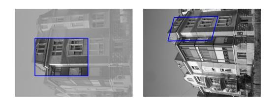
10 10 Simon Korman et al. Fig. 12 Zurich Dataset [22] - the remaining: Failures (row 1), Occlusions (row 2), Template or Target template is out of plane/image (row 3) Fig. 11 Zurich Dataset [22] - Good Examples: In the blue rectangle on the left of each pair of images is the template presented to FastMatch. In the blue parallelogram on the right is the region matched by the algorithm. Note that also for some of the non-affine mappings Fast-Match gives a good result. area in the target image, the more demanding the overlap error criterion becomes9. This is relevant especially to the zoom sequences. The Wall images are uniform in appearance and this makes it difficult to translate good SAD error to correct localization. The results of Experiment II can not be compared with those of [14] as they do not deal directly with template or image matching. In this experiment too, Fast-Match deals well with photometric changes as well as the blur and JPEG artifacts. 5.3 Matching in Real-World Scenes In the third experiment, we present the algorithm s performance in matching regions across different view-points of real-world scenes. We use pairs of images from the Zurich buildings dataset [22]. As done in the second experiment, we choose a random axis-aligned rectangle in the first image, where the edge sizes are random values betwee0% and 50% of the respective image dimensions. This dataset is more challenging for the performance of the algorithm, as 9 This issue has been extensively discussed in [15]. well as for experimentation: The template typically includes several planes (which do not map to the other image under a rigid transformation), partial occlusions and changes of illumination and of viewpoint. As there is no rigid transformation between the images, we evaluated the performance of fast match on 200 images visually. O29 of these we found that the mapping produced by the algorithm was good, in the sense that it corresponded almost exactly to what we judged as the best mapping. In most of the remaining cases producing a good mapping from the given template was impossible: On 40 of the images, the location corresponding to the template was not present in the other image, or that the template spanned several planes which can not be mapped uniquely. I2 of the images the location that the template was a photograph of was occluded by some outside element, such as a tree. In only 19 of the images was locating the template possible, and the algorithm failed to do so. Examples of good mappings can be found in Figure 11. Examples of cases where a good match was not found appear in Figure 12. The results on the entire dataset appear in [11]. 6 Conclusions We presented a new algorithm, Fast-Match, which extends template matching to handle arbitrary 2D affine transformations. It overcomes some of the shortcomings of current, more general, image matching approaches. We give guarantees regarding the SAD error of the match (appearance related) and these are shown to translate to satisfactory overlap errors (location related). The result is an algorithm which can locate sub-images of varying sizes in other images. We tested Fast-Match on several data sets, demonstrating that it performs well, being robust to different real-world conditions. This suggests that our algorithm can be suitable for practical applications. An interesting direction for future research is to apply similar methods to more diverse families of transformations (e.g. homographies) and in other settings, such as matching of 3D shapes.

11 FAsT-Match: Fast Affine Template Matching 11 Appendix - Proof of Theorem 1 We first restate Theorem 1 for completeness: Let I 1, I 2 be images with dimensions and n 2 and let δ be a constant in (0, 1]. For a transformation T, let T be the closest transformation to T in the net N δ (which is a δ n2 1 - cover). It holds that: T (I 1, I 2 ) T (I 1, I 2 ) O(δ). To understand why the claim holds we refer the reader to Figure 13. Two close transformations T, T map the template to two close parallelograms in the target image. Most of the error of the mapping T is with respect to the area in the intersection of these parallelograms (the yellow region in Figure 13). This error cannot be greater than the total variation multiplied by the distance between the transformations T and T, as shown below. The rest of the error originates in the area mapped to by T that is not in the intersection (the green region). The size of this area is also bounded by the distance between the transformations. Thus, the distance between the transformations, and the total variation, bound the difference in error between T and T. This is formalized in the remainder of the section. For convenience, throughout the discussion of the algorithm s guarantees we consider points in a continuous image plane instead of discrete pixels. Analyzing the problem in the continuous domain makes the theorem simpler to prove, avoiding several complications that arise due to the discrete sampling, most notable, that several pixels might be mapped to a single pixel. We refer the reader to a (slightly more involved) proof in the discrete domain, which we made available in a previous manuscript [10]. In order to switch to the continuous domain, we give some definitions and state some claims for points in the image plane. We begin by relating the intensity of points to that of pixels. Definitio The intensity of a point p = (x, y) in the image plane (denoted I 1 (p)) is defined as that of the pixel q = ([x], [y]), where [ ] refers to the floor operation. The point p is said to land in q. We now define the variation of a point and relate it to the variation of a pixel. Definition 2 The variation of a point p, which we denote v(p), is max q : d(p,q) 1 I 1 (p) I 1 (q). Note that this is upperbounded by the variation of the pixel that p lands in. For convenience of computation (this does not change the asymptotic results), for points p that have a distance of less tha from the boundary of the image, we define v(p) = 1. Finally, we define the total variation of an image in terms of the total variation of points in the image plane. Definition 3 The total variation of an image (or template) I 1 is I 1 v(p). We denote this value. Note that this is upper bounded by the total variation computed over the pixels. Fig. 13 A template mapped to an image by two close transformations. The close transformations map the template to close parallelograms. The error of T cannot be very different from that of T. Most of the change in error is from different points being mapped to the intersection area (in yellow). This difference depends on the total variation of the template. The remaining error depends on the green area which is small because the transformations are close. Our strategy towards proving Theorem 1 involves two ideas. First, instead of working with the pair of transformations T and T, we will more conveniently (and we show the equivalence) work with the identity transformation I and the concatenated transformation T 1 T. Second, note that in Theorem 1, we bound the difference in error between transformations T and T, which are δ apart. A simplifying approach, is to relate the transformations T and T through a series of transformations {T i } m i=1 (where T 0 = T and T m = T ), which are each at most at a unit distance apart, with m = O( δ n2 1 ). Thus, in Claim 6 we handle the case of transformations that are a unit distance apart. In the following lemmas we introduce a constant u, such that if l (T, T ) u it holds that l (T 1, T 1 ) 1. Claim 4 Given affine transformations T, T with scaling factors in the range [1/c, c] such that l (T, T ) fracδ n 2 1, it holds that l (T 1, T 1 ) = O( δ n2 1 ). Proof To see that the claim above holds, consider a point q and we will show that T 1 (q) T 1 (q) c δ n2 1 (see Figure 14). Let p = T 1 (q) and let p = T 1 (q). We wish to bound p p. Let r = T (p ). We get p p = T 1 r T 1 q = T 1 (r q) c r q c δ n2 1. Claim 5 There exists a value u (0, 1) such that for any affine transformations T, T where l (T, T ) u and for any point p I 1, it holds that p, T 1 (T (p)) 1. The correctness of Claim 5 follows directly from Claim 4 by noting that p = T 1 (T (p)). Claim 6 Let I 1, I 2 be images with dimensions and n 2. There exists a constant u (0, 1) for which the following holds. For any two affine transformations T and T such that l (T, T ) u: ( ) T (I 1, I 2 ) T (I 1, I 2 ) O 2