Excel 2000 MICROSOFT. Level 3. Version N2

Transcription

1 MICROSOFT Excel 2000 Level 3 Version N2 ICT Training First Floor Victoria House Queen Alexandra Hospital Cosham PO6 3LY Tel: ext: ICT.Training@porthosp.nhs.uk Website: ICT TRAINING has made every effort to ensure that the material in this manual was correct at the time of publication but cannot be held responsible for any errors or inaccuracies. ICT TRAINING reserves the right to change or replace information contained in the manual without notice. For the most up to date version please refer to the ICT Training website.

2 CONTENTS 1. GENERAL COURSE INFORMATION HIDE AND PROTECT CELLS AND FORMAT CELL DATA TYPE Hide/Unhide Cells Cell and Workbook Protection Protect a worksheet Protect a workbook To remove the protection for a worksheet or workbook CREATE A SHARED WORKBOOK How to create a shared workbook Using a shared workbook PIVOT TABLES Editing Pivot Tables Pivot table Layouts The summarize by tool Showing certain fields Viewing related information Grouping data Creating charts from Pivot Tables ADD DATA RESTRICTIONS AND MESSAGES TO DATA Comments Validation ADVANCED LOOKUP THE CONCATENATE FUNCTION THE VALIDATION DROP DOWN LIST VLOOKUP FUNCTION ADVANCED FORMULAE AND FUNCTIONS IF Function Nested If functions IFAND DATEIF SUMIF DSUM...28

3 11. FORMS CUSTOMISING MENUS AND TOOLBARS 'Personalized' menus and toolbars in Excel Creating a personalised toolbar AUTOMATING COMMON TASKS USING MACROS What is a macro? Running a macro FAULT REPORTING Out of office hours ICT TRAINING CANDIDATE APPEALS PROCEDURE VERSION CONTROL/LOG...39

4 1. GENERAL COURSE INFORMATION COURSE TITLE METHOD OF TRAINING DURATION PRE-REQUISITES EXCEL 2000 LEVEL THREE Classroom 3 hours Excel 2000 Level Two ABOUT THE COURSE This course covers the skills necessary to produce Excel spreadsheets. It allows the attendees hands on practical experience withthe help and guidance of a trainer. SUITABLE FOR Those who are familiar with Microsoft Excel's functionality and who have completed the Excel Spreadsheets Level 2. OBJECTIVES This course will enable the student to: 1. Hide and protect cells 2. Create a shared workbook 3. Create and use pivot tables to filter data 4. Add data restrictions and messages to data 5. Use data validation 6. Advanced formulae and functions 7. Customising menus and toolbars 8. Automating common tasks using macros 4

5 2. HIDE AND PROTECT CELLS AND FORMAT CELL DATA TYPE 2.1. Hide/Unhide Cells Function Hide/Unhide a column Hide/Unhide a formula Hide/Unhide a row Hide/Unhide a sheet Protect workbook Protect Worksheet Unlock/Relock cells Method Format, Column, Hide or Unhide Format, Cells, Protection tab, select/deselect Hidden check box Format, Row, Hide or Unhide Format, Sheet, Hide or Unhide Tools, Protection, Protect Sheet, assign optional password Tools, Protection, Protect worksheet, assign optional password Format, Cells, Protection tab, deselect/select Locked check box Note: some of the hide and protect options do not take effect until protection is enabled Locked This function prevents selected cells from being changed, moved, resized, or deleted. Locking cells has no effect unless the sheet is protected. To protect a sheet, point to Protection on the Tools menu, click Protect sheet, and then select the Contents check box. 5

6 Hidden Hides a formula in a cell so that it doesn't appear in the formula bar when the cell is selected. If you select this option, it has no effect unless the sheet is protected. To protect a sheet, point to Protection on the Tools menu, click Protect sheet, and then select the Contents check box, as shown above Cell and Workbook Protection If you have a workbook which is used by others, to may want to protect it so that important data is not accidentally altered or lost. You can protect all or part of the workbook. It is also possible to make these worksheets password protected, so that users would need a password to gain access or to alter certain worksheets and workbooks. You can protect a specific worksheet against changes to cell contents, objects or scenarios or you can protect the entire workbook so that it is not possible to insert or remove sheets, change the window size etc. If users are to be able to change the contents of selected cells in a protected worksheet, these cells have to be locked before the sheet is protected. For extra security a workbook can be given a password, which when entered will open the protected workbook. When a protected sheet is opened a password box like the one below will appear: To specify cells which are not be write-protected 1. Select the desired cell or range 2. Right-click the selected cell or range and choose Format Cells from the shortcut menu 3. Choose the Protection tab 4. Uncheck the Locked box and choose OK 2.3. Protect a worksheet 1. Choose the Tools/Protection/Protect Sheet menu item 2. Specify what is to be protected under Protect worksheet for 3. If necessary, enter a password and choose OK 4. If necessary, re-enter the password and choose OK 2.4. Protect a workbook 1. Choose the Tools/Protection/Protect Workbook menu item 2. Specify what is to be protected under Protect workbook for 6

7 3. If necessary, enter a password and choose OK 4. If necessary, re-enter the password and choose OK 2.5. To remove the protection for a worksheet or workbook 1. Choose the Tools/Protection/Unprotect Sheet or Workbook menu item 2. If necessary enter a password and choose OK 7

8 3. CREATE A SHARED WORKBOOK To allow several users on a network to work on the same workbook simultaneously, you must share it How to create a shared workbook 1. Open the workbook that you want to share 2. Tools > Share Workbook 3. Click the Editing tab 4. Activate the Allow changes by more than one user at the same time option. You can see the names of the users who are currently working with the workbook, in addition to the date and time they opened the workbook. 5. Click OK. Excel asks you to save the workbook so click OK If you have not already done so, you now need to make the shared workbook available to other users by saving it on the network where other users can access it. To do this, use File > Save As. By doing this you make a copy of the shared workbook. The name of the workbook appears on the title bar, followed by the word Shared Using a shared workbook Open the workbook concerned You can add data, insert rows, columns, sort the data, but you cannot delete worksheets, define conditional formatting, merge cells, insert charts, objects or hyperlinks. To find out who the other users are, use Tools > Share Workbook, and click the Editing tab. The Advanced tab gives more options concerning saving and maintaining a shared workbook. To change a workbooks status so it is no longer a shared workbook, go to tools, shared workbook 8

9 and remove the tick from the allow changes by multiple users. 9

10 4. PIVOT TABLES Occasionally you will want to create a report summarising the data in a spreadsheet. Your report will probably perform a particular type of calculation using the data. You might even want to filter the data you include in a particular calculation. Where the spreadsheet you are working with are large and detailed, creating a summary report can be a complicated and demanding task. Excel s PivotTable functionality allows you to create dynamic, interactive summaries of a set of data. You can change what information is shown in a pivot table by simply clicking the drop down arrow and selecting and deselecting different options. Below is an example of a pivot table, it shows the category and method fields from the source data, from which the pivot table has been created. Source Data Pivot table report A PivotTable can quickly be reorganised by dragging a field to another section of the PivotTable. All data and totals will automatically be updated. In addition it is possible to show subtotals, change the summary function or choose custom calculations for the PivotTable. Page Field Column Field Data Field Row Field Grand Total To create a PivotTable, you must specify the data to be used as row fields, column fields and page fields and the data to be calculated in the data range. The way in which data is displayed in a PivotTable can vary, depending on which fields and items are included from the source data and their position in the table. 10

11 A PivotTable is created using the PivotTable and PivotChart Wizard which provides step-by-step help in choosing source data and the layout for the PivotTable. 1. Open the workbook that contains the data and place the cursor in the list of source data 2. Show the PivotTable Toolbar 3. Click the PivotTable Wizard button 4. Select Microsoft Excel list or database and PivotTable in the first step of the wizard then choose next. In the second step you have to specify the range containing the source data. As the cursor is place in the list, the wizard automatically chooses the entire list as the range. 5. Make sure that the correct range is chosen then choose next. In the third step you specify the position of the PivotTable. If you choose Existing worksheet you will need to type a cell address as the position of the table. 6. Click Finish 11

12 An empty PivotTable is inserted in the specified range and the PivotTable Toolbar now has separate buttons for the relevant fields. The PivotTable is created by dragging the desired column and row fields to the correct positions in the table. The PivotTable is completed when fields are dropped into the Drop Data Items Here field Editing Pivot Tables The pivot table can be altered to show different results by simply dragging a data source out of the table area and dragging a new data source in or adding another data source to existing ones, as shown here: 12

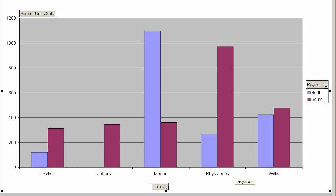
13 4.2. Pivot table Layouts The layout of the pivot table can be altered using the same technique, rows and column headings can be moved around to change the look of the table: If the source data is changed, a PivotTable can be refreshed without it needing to be created from scratch. New records added and inserted at the end of the list will not be show in the PivotTable. The data range for the PivotTable must be changed for these records to be included as well. To update the pivot table data right click over the pivot table and select refresh data from the popup menu, or click the refresh data button on the pivot table toolbar The summarize by tool As well as the table layout, you can also change how the tables contents is summarized. A pivot table shows it s results by summarizing the data within the original list. Pivot tables default to the sum function, but you can also summarize the data by count, average, max and min for example. The example below shows a table which is summarized by sum. This can be changed by double clicking the area which say s Sum of units sold. The box shown below will then appear. Simply select a new way to summarize your table from the list and select Ok. The table will then show the data summarised in the new way. Original table layout Altered table layout 13

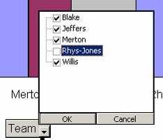
14 4.4. Showing certain fields You can also edit the table to show certain data within a field. For example if you just want to view the totals from only certain team members rather than the whole body of staff, you can do so. Simply select the drop down list next to the field name and remove the tick by clicking once from all the data sources you don t want to view, and select OK. The table will now be showing information concerning only the data sources which you want to see Viewing related information By double clicking on a cell a new sheet is inserted into your file containing relevant information to the cell you selected. By double clicking on the cell which contains a sale for the team member Blake in the central region, a new sheet is inserted showing all the sales Blake has made within the Central region. 14

15 4.6. Grouping data Data within a pivot table can be grouped. The example on the right shows the individual sales from members of a team. If two members began working together, their data could be grouped together in the pivot table to illustrate this. For example, if you wanted to group together the team members Blake and Rhys-Jones, you would firstly select the cell containing Blake s name, hold down Ctrl and then select the name Rhys-Jones. Right click over the cells you have just selected and on the popup menu select the option Group and Outline, then select Group from the submenu. The pivot table will now show the team members as part of a group as illustrated below: 4.7. Creating charts from Pivot Tables Charts can be created from a pivot table by simply selecting the chart wizard button on the pivot table toolbar. A new sheet will automatically be inserted into the workbook containing a chart showing the details currently showing in the pivot table. The chart can be altered to show different data in the same way a pivot chart can, simply by clicking the field drop down list and selecting what data to show in the charts. The charts type, titles and legends can all be editing by clicking the chart wizard button in the chart sheet. 15

16 16

17 5. ADD DATA RESTRICTIONS AND MESSAGES TO DATA 5.1. Comments Occasionally it may be necessary to write comments or tips on data in a worksheet. Comments can be inserted on yellow notes in the workbook without making changes to the cells themselves. Cells which contain comments have a little red symbol in the top right corner To Show or hide the Reviewing toolbar right click the toolbar area and choose Reviewing from the shortcut menu. To insert a comment click New Comment on the Reviewing Toolbar Use the Reviewing toolbar to go to the next or previous comment, edit a comment, delete a comment or show/hide a comment. Format comment text by first using edit comment, selecting the text then right-clicking and choosing Format Comment from the shortcut menu. 17

18 5.2. Validation Using the Validation tool allows you to specify rules that control what data the user can enter. Select the cell or range to have validation applied. Use the Data > Validation menu option Choose the data type and apply any additional criteria; for example, when selecting the whole number option, you can choose from a range of operators, minimum or maximum values. If you choose the list option, you must nominate an Excel range that contains values to populate a dropdown list Move to the Input Message page. The text that you supply in the title and message areas is displayed whenever the user clicks into a cell containing this validation. Move to the Error Alert page. The text that you enter here is displayed whenever the user violates the validation rule that you have set. Note that there are 3 styles of error message. The example shown first is the warning style. Shown below are examples of the stop and information styles. 18

19 6. ADVANCED LOOKUP You can create quite an advanced lookup system by combining several commands together. This is useful if you have a large list of data which you need to search. The example below shows a system which combines the vlookup function with a validation list and a text function called CONCATENATE. By using this system the user can lookup all the relevant details about a person by selecting their name from the drop down validation list, which is shown in cell A2 in the example. Lookup area List of data A1 = Contains a drop down validation list. B2:G2 = Contains the vlookup function A1:G2 = The lookup area C7:C22 = Contains the concatenate function A7:I22 = The list of data The text function concatenate, allows you to combine piece of text together, so if you had a persons firstname and surname in different columns, you could create a new column within your list that contains the concatenate function. This would add the first and surnames together so that you could search the list by full name, rather than by surname only, which could produce duplicate results. The validation list would then allow you to create a drop down list of the full names within the list, within the lookup area of your spreadsheet. The vlookup function looks up information in a large list so you avoid having to manually search for the data you are looking for. 19

20 7. THE CONCATENATE FUNCTION The concatenate text function allows you to add together different cells that contain text. For example, if one column within the list contains a persons firstname, and another column contains a persons surname, you can add another column to your list containing the concatenate function and add the two cells together. This makes it easier and more accurate when searching for information when combined with a drop down validation list. The concatenate function looks like this: =CONCATENATE(B8," ",A8) B8 = Is the cell within the list which contains the persons firstname = Is a space contained within speech marks. (This is so a space will appear between the two pieces of text.) A8 = Is the cell within in the list that contains the persons surname This function can then be copied to any other cells in the normal way. A Validation drop down list can then be created using this new column containing the concatenate function as a reference. See page 21 for information on Data Validation. 20

21 8. THE VALIDATION DROP DOWN LIST In the example we have been using, the spreadsheet contains a lookup area where the information you re a searching for is displayed. In this case the vlookup will only work when there is a lookup value entered. In this example our lookup value is the full name of a person. This could be manually typed in but to avoid any spelling errors you can create a drop down list containing all the full names of the people in the list so that the user will only need to select a name from the drop down list. 1. Select the cell you want the drop down list to be in, this will be in the first cell within your lookup area. 2. Select the validation option from the data menu 3. The data validation box will open. Select the settings tab and in the allow drop down list select the list option. 4. In the source area enter the cell range that contains the information that you want to appear in the drop down list, by clicking and dragging over the appropriate cells. 5. Click Ok. A drop down list will now be active in the selected cell. Any name from the list could be selected and the relevant information for that person will show in the area where the vlookup function is entered. 21

22 9. VLOOKUP FUNCTION The lookup function used in this example is: =VLOOKUP(A2,C7:I22,2,FALSE) A2 = The cell containing the chosen name we are looking for C7:I22 = The original list of data we are searching. (The columns containing the surname and firstname are not recognised as part of the table due to the fact that the column containing the concatenate function is seen as the first column of the list) 2 = The column we are searching within the original data list. False = So only the exact match is found and displayed. 1 st column of the list This function is entered in cells separate from the original list of data, where you want the information retrieved from the original list to be displayed. The cell references within the function will stay the same, apart from the column reference (shown above as 2 within the function) which will change depending on what column within the original list of data, we want to search. For example in the image above, column B shows the data of birth of a person. This is the second column within the original data list, (the columns containing the surname and firstname are not recognised as part of the table due to the fact that the column containing the concatenate function is seen as the first column of the list) hence why 2 is inserted in the function. In this example below, the column number has changed from 2 to 3, this is because we are looking for the persons doctor which is contained in column 3 of the original data list. =VLOOKUP(A2,C7:I22,3,FALSE) 3 rd column of the list 22

23 10. ADVANCED FORMULAE AND FUNCTIONS IF Function An if function, allows you to test a cell for two scenarios, and what will happen if it is true and what will happen if it is false. If the test proves true, one action is performed if false, a different action is performed. The action could be a calculation, or it could be adding in a value or text into the cell. The function is split into three areas: 1. The Condition (i.e. the test of the cell value) 2. What will happen if it is true 3. What will happen if it is false In the example shown below, we want to give a bonus of 10% if a salesman has made sales over 1000, however, if the amount is under 1000, we want the cell to state that no bonus is given. The condition being tested for is: If the value in the total sales cell is greater than 1000 the value in this cell is to be multiplied by 1%. If the test proves false, the text No bonus is to be inserted into the cell instead. This formula will be in the Bonus cell. (G3) =IF(F3>1000,F3*10%,"No Bonus") Note that the three arguments are within brackets, separated by commas: The condition: F3>1000 Tests whether F3 is greater than 1000 (no sign needed) If TRUE works out 10% of the amount in F3 that is over 1000 If FALSE displays the text No Bonus When entering any text into a formula all text entered has to be inserted between speech marks like this: No Bonus. No spaces are added to the formula, as commas are used to separate the different conditions and actions 23

24 10.2. Nested If functions A nested IF function works in the same way as a normal IF function does, but it allows you to give more than one true condition. In the previous example the condition was that if a salesman had total sales over 1000, they would receive a 10% bonus. We can build on this scenario for our nested IF function. If we needed to give the salesman one bonus for getting over 800 total sales, and a bigger bonus if they got more than 1000 sales we would have to create a nested If function. The formula would look like this: =IF(F3>1000,F3*15%,IF(F3>800,F3*10%,"No Bonus")) Condition 1: F3>1000 = this tests whether the value in F3 is greater than 1000 If this is true: F3*15% = Will work out 15% of the amount in F3 that s over 1000 Condition 2: F3>800 = this tests whether the value in F3 is greater than 800 If this is true: F3*10% = Will work out 10% of the amount in F3 that s over 800 If any of the values do not fit these statements (i.e. if any of the total sales are less than 800) then: False: No Bonus = the cell will display the text No Bonus. The highest bonus ( 1000 = 15%) needs to be entered into the function first, with the lower bonus entered afterwards. If this were not done, Excel would not be able to calculate the bonus correctly. =IF(F3>1000,F3*15%,IF(F3>800,F3*10%,"No Bonus")) Highest: 1000 & 15%, Lowest: 800 & 10% 24

25 As before any text entered into the formula has to be entered within speech marks like this: No Bonus. There are no spaces within the formula and commas are used to separate the different conditions and actions IFAND The If function can be combined with other functions to make a more complex formula which allows you to analyse data to a greater scale. Here I want to return the number 1 if the Surname is Anderson and the Type is Advanced. 1. Select the cell you want the formula to appear in. 2. Click the function button and select If from the function list. 3. Before you type any arguments, immediately start the And function by clicking the drop down arrow within the formula bar: (If it is not in the list, go to More Functions and find it there.) 4. The And Function will open. Enter the Arguments: (Text needs to be in quotation marks) 25

26 You now need to go back to the If function. Click the word IF in the formula bar: Enter the Values for true and false and replicate the formula down as required. 26

27 10.4. DATEIF You may need to calculate the number of days which have elapsed between one date and another. In this case you would use the DATEIF function. =DATEDIF(B1,B2,"D") B1 = Refers to the cell with the first date. B2 = Refers to the cell with the last date. D = Refers to the time element involved which is days. If you want to calculate the time in months replace the D with an M in the formula, and if you want to calculate the years, replace it with a Y SUMIF The SUMIF function adds a range of values together when a specific criteria is defined. For example if you had a list of different drinks along with the amount sold for each, and you wanted to calculate only the amounts sold for one type of drink, you would use the sumif function. The example below shows a list containing different types of drinks and the total of each. The total figure in B9 is showing the total for Coke only. The total is calculated by the formula: =SUMIF(A2:A7,B8,B2:B7) A B 1 Drink Total 2 Coke 44 3 Fanta 66 4 Fanta 23 5 Coke 89 6 Sprite 12 7 Sprite 43 8 Drink: Coke 9 Total: 133 A2:A7 : The range of cells in which to look for the criteria B8: The cell containing the criteria s value B2:B7 : the range of cells to add up if the value is TRUE (i.e. if the cell values and the criterion value matches) The criteria in B8 can be changed and the formula will update to show the new results, for example if you were to replace the word coke with sprite, the formula would calculate the totals for sprite. 27

28 Exercise: Create a SUMIF function to calculate the amount of apples using the table below: A B 1 Produce type Total sold 2 Apples 52 3 Pears 45 4 Oranges 21 5 Apples 56 6 Apples 82 7 Oranges 53 8 Pears 16 9 Apples Produce: 11 Total: DSUM Functions are a set of instructions/calculations which allows Excel to find specific information within a range of data. The functions used in excel databases are constructed in a similar way to regular Excel functions, and are indicated as being database functions by incorporating the letter D at the beginning of the function name. These database functions can be used to define specific data within an excel database list. These functions are: DSUM DAVERAGE DMIN DMAX adds up a list of values averages a list of values finds the minimum value in a list finds the maximum value in a list The functions are almost the same as regular excel functions, the difference being that the letter D is incorporated into the function name and that there are more cell references needed within the function to calculate the result. These cell references can either be a single cell reference, a cell range or a named area. Broken down the DSUM looks like this: =DSUM (database area, Field name, criteria area) A1:D24: The range of cells which contain the complete database area. D1: The field name (i.e. the total column) F1:F2: The area where the criteria is entered. 28

29 In the example below we are searching for the summed total for the East area only. A1:D24 = the complete range of cells within the database list D1 = the heading of the column we want to calculate, this must be entered into the function enclosed in double quote marks. In this case we want to sum the totals; therefore the total column heading is the field name. F1:F2 = the range of cells which contain the criteria, this needs to include the column heading of our search criteria and the criteria itself, so in this example this is the column 29

30 title Region and the criteria, and as we are summing the totals for the East area only, search criteria is East. G6 = This cell shows the result of our DSUM function; the overall summed total of all the total results for the East. By having a criteria area which is separate to the table, the criteria can be changed and the function will update itself automatically. 30

31 11. FORMS By using a data form you can find and edit specific records easily. Click within your list and then select Data from the main menu and then the Form option. A form will appear over your data list, displaying the first record. The number of records is displayed at the top of this form. By using the relevant buttons you can add a New record or Delete the one displayed. If you select the Criteria button you can find a specific record. The form becomes an entry form so you can enter the values of the record you wish to find. By clicking next after entering your criteria the form will jump to any matching records within the list. Keep clicking Find Next to step through each similar record Comparison operators can also be used to find a specific record: > Greater than < Less than <> Not equal to >= Greater than or equal to <= Less than or equal to If no operators are used, it is assumed to be Equal To the entered value. Click Clear to delete criteria and start again and click Form to finishe searching and return the normal form screen. 31

32 12. CUSTOMISING MENUS AND TOOLBARS 'Personalized' menus and toolbars in Excel 2000 From a standard Excel 2000 installation, as you navigate the new menus and toolbars you see that the menus are shorter than they were in previous versions and the toolbars change in appearance from time to time all on their own. The idea is that Excel 2000 displays only the commands you use most often on the new personalized menus and toolbars. So you just see a short (abbreviated) menu at first and you can expand menus to reveal all categorised Office commands by clicking a little expansion bar in the menu that becomes a spacer. After you click a menu command, it appears on your short personalized menu. Toolbars share space in a single row so that more screen space is available for your work. When you click a button on a toolbar, that button is added to the personalized toolbars on your screen. You can also customize toolbars in the same way as in previous versions of Office. Left: The abbreviated Excel - Edit menu as you click the Edit menu command. Right: the full length menu after you click the expansion icon (fast forward symbol). Expansion icon. If you were to select the Replace menu item, the next time you launch the Format menu it includes that item in your abbreviated menu; see below. 32

33 Office assumes you would like this option on your abbreviated menu 33

34 To turn off the abbreviated/dynamic menus. 1. Select View, Toolbars, Customize. 2. In the upper area of the Customize dialog box, uncheck the Menus show recently used commands first check box Creating a personalised toolbar 1. Select Tools from the main menu and then select customize from the tools drop down list. 2. Then select the toolbar tab in the customize box. 3. Click the New option. You will be prompted to give the new toolbar a name, click OK when you have done this. A toolbar with no command icons will appear. It can be moved and used in exactly the same way you normally use toolbars. We now need to add command icons to our toolbar. 4. Click the toolbar drop down arrow, select the add and remove option and then the Customize option. 5. You will be returned to the customize box, this time select the commands tab. 6. Click on the command you want to add and drag onto your new toolbar. The chosen command icon will now appear on your toolbar. 34

35 You can choose any menu category from the list and the command icons will change to reflect the chosen menu. Thus allowing you to have command icons from various toolbars all contained on one toolbar. Command icons can be rearranged on your toolbar by clicking and dragging the icon to a new position. You can change the image of your icon by right clicking on a command icon, and selecting the change button image from the drop down list. The following picture pallet will appear from which you can assign any of the imagery to your command icon. Altered command icon: You can also add text to the altered command icon to make the toolbar easier to use, by using the drop down list. NOTE To alter a toolbar s appearance, the customize box must be open. You will not be able to alter a toolbar by right-clicking otherwise. Even macros can be created and assigned to a toolbar with a command icon. See page 36 on how to create a macro. 35

36 13. AUTOMATING COMMON TASKS USING MACROS What is a macro? In Excel, tasks can be automated using macros. A macro is a series of actions which are stored in a Visual Basic module, and which can be run when the task is to be performed. 1. Open the workbook 2. Tools > Macro > Record New Macro 3. Type the name of the macro in the Macro name box 4. Indicate, if necessary, the shortcut key that will run the macro. 5. Indicate where the macro should be recorded: in This Workbook (if the workbook is open) or in a New Workbook. If the macro is to be available all the time, choose Personal Macro Workbook. 6. If necessary, enter text in the Description box to change or add to the information about the macro. 7. Click OK The macro toolbar (with two tools) appears as well as the word Recording on the status bar. 8. Carry out the action you want to record in the macro. Once all the actions have been completed, click the Stop Recording button on the macro toolbar Running a macro 1. If the macro was recorded in a workbook or other than Personal.xls, open the workbook. 2. Open the workbook in which you want to run the macro. 3. Tools>Macro>Macros or Alt+F8 4. Indicate where the macro you want to run is saved, using the Macros in list 5. Double-click the macro you want to run. 36

37 14. FAULT REPORTING Contact ICT Service Desk: PHT network users phone or SJH (7703) Some of the reasons you may need to contact the ICT Service Desk: EQUIPMENT FAILURE SOFTWARE PROBLEMS SCREEN FREEZES PASSWORD NON-ACCEPTANCE * You will need to give the Service Desk certain information, so always ensure you have the following information available. They may need to know: Your Username. The KB Number of the equipment. This is found on a small label (usually red or blue) stuck to the equipment. The function set and function you were working in. The patient s details e.g. casenote no. Exactly what you were attempting to do, e.g. log on, admit patient, register patient Out of office hours Contact the ICT Service Desk and leave a message on the answer machine. They will deal with the problem as soon as they can. Alternatively them. If you feel there is a major system problem contact the switchboard for them to contact the engineer on call. 37

38 15. ICT TRAINING CANDIDATE APPEALS PROCEDURE Candidates who are unhappy with any aspect of the end of course/test assessment decision should first discuss the problem with the ICT Trainer at the time of receiving the result. The reasons must be made clear by the candidate at this time. If the candidate is still unhappy with the result further discussion should take place involving the ICT Training Team Leader or ICT Training Senior Trainer within 3 days of the course/test date. The ICT Training Department will keep a record of such discussion together with date and outcome. Where necessary the 1 st marker will be asked to re-mark and the marking checked by the ICT Training Team Leader or Senior Trainer. It should be noted that if the candidate was borderline double marking should already have been undertaken. If this does not provide satisfaction the candidate may raise a formal appeal. Appeals will only be accepted if made in writing (not ) to the ICT Training Audit & Quality Manager within 10 days of the candidate receiving their result, outlining clearly the circumstance of the appeal. The 1 st & 2 nd markers will meet with the Training Audit & Quality Manager to consider if there are any aspects that should be taken into account in the candidate s performance. In some circumstances the candidate may be offered a re-test (e.g. hardware or software problems). If this is not the case and the result remains unchanged and the Training Audit & Quality Manager is unable to resolve the impasse then the candidate may write to the ICT Training Manager (within 5 days of receiving the 3 rd result) who will consider all evidence and circumstances of the appeal also taking into consideration responsibilities to the Trust and Data Protection Act to make a final decision. ICT Training QAH July

39 16. VERSION CONTROL/LOG Manual Excel 2000 Level Three Version V.N2 Date July 2008 Revisions Page Updated Formatting and text refinements (unlisted as content and ALL meaning unchanged) NEW Course Outline 4 Updated Protection new image 5 Updated Shared Workbook text and image 8 Moved Advanced Functions reordered in manual 19 NEW Fault Reporting 37 NEW Candidate Appeals Process 38 NEW Version Control/Log 39 Removed Conditional Formatting moved to level 2 manual - 39