SECTION - B MS-EXCEL 2010

Transcription

1 SECTION - B MS-EXCEL 2010

2 C R1 Office automation-ms-excel INTRODUCTION 2010 H TO A P MS-EXCEL 2010 T E LEARNING OBJECTIVES To understand the basics of spreadsheet application To create a worksheet file To enter and edit data in the worksheet file 1.1 INTRODUCTION TO MS-EXCEL A Spreadsheet is a computer application that simulates a paper worksheet. It displays multiple cells that together make up a grid consisting of rows and columns, each cell containing either alphanumeric text or numeric values. A spreadsheet cell may alternatively contain a formula that defines how the contents of that cell is to be calculated from the contents of any other cell (or combination of cells) each time any cell is updated. Spreadsheets are frequently used for financial information, because of their ability to re-calculate the entire sheet automatically, after a change to a single cell is made. Examples of popular spreadsheet software are MS-Excel, Gnumeric, KSpread, ZCubes-Calci, Lotus Symphony (2007) and Resolver One. Microsoft Excel consists of a proprietary spreadsheet application written and distributed by Microsoft. Excel 2010 needs Windows Vista or Windows 7 as operating system to run on an IBM PC. However, it can also be used with Windows XP operating system, if service pack 3 is installed. MS-Excel features calculation, graphing tools, pivot tables and, a macro programming language called VBA(Visual Basic for Applications). A typical blank Microsoft Excel 2010 spreadsheet is shown in the Fig Fig : A typical blank Microsoft Excel 2010 spreadsheet 184 INFORMATION TECHNOLOGY

3 Introduction to MS-Excel 2010 Excel also allows multiple sheets, so a spreadsheet could be split over several pages, say one for input, one page for calculations, and another for output. This collection of pages is known as a Workbook. By default, a workbook opens with three worksheets and it can contain a maximum of 255 worksheets. In addition to powerful calculations, Excel is also able to produce a wide range of high quality charts to make presentation of data more effective. Spreadsheet programs are developed to automate tasks such as technical calculations, inferential statistics, analyzing data etc. They also have a powerful program for graphical preparation of numerical data. They are commonly used in Production, Planning, Personnel Management, Marketing, Payroll and Accounting. Moving Around an Electronic Spreadsheet : Users can move the cursor around the electronic spreadsheet, changing the current cell. Most spreadsheets allow many more rows and columns than can be displayed at a time on the screen. If the user moves the cursor off the screen, the program will reveal columns or rows that were previously kept in memory but not displayed on the screen. Entering Data on an Electronic Spreadsheet : To enter data into a cell, the user can move the cursor to the cell and type in the data. If the data consists of a formula, the formula appears only at the top of the screen and not in the cell itself. The electronic spreadsheet automatically calculates the value of the formula and inserts the value into the cell. At the same time, the values of all other cells that depend on the value of the current cell are recalculated. Changing the Content of a Cell : To change the content of a cell, the user must move the cursor to the cell and enter the new content. The old content of the cell is lost, and the new cell value is inserted (or computed, if the new cell value is determined by a formula). Any cell values that depend on the value of the changed cell are recalculated. This ability to change the content of a cell easily and to see the effects of the change on the other cells in the spreadsheet immediately is what makes electronic spreadsheets so useful. Editing the Electronic Spreadsheet : Electronic spreadsheets allow the user to save the current contents of the spreadsheet on a disk and to recall the spreadsheet at a later time. They also include a number of editing features that make it simpler to create and change spreadsheets. The editing features allow the user to erase the content of a single cell or of an entire rectangular block of cells. They allow the user to add or remove rows or columns, and they automatically adjust the formula from one cell to another. The editing features even allow users to merge spreadsheets and to add and subtract spreadsheets on a cell by cell basis. They also make it simple to enter or alter the data in the cells. Spreadsheets are too large to appear completely on the screen. A number of editing features compensate for this limitation. One such feature, Freeze Panes freezes titles on the screen so that when the user brings a remote section of the spreadsheet onto the screen, the horizontal or vertical titles remain on the screen. 1.2 SPREADSHEET DETAILS Worksheet is a grid made up of horizontal rows and vertical columns. The Excel 2010 worksheet contains 1,048,576 rows and 16,384 columns.each intersection of a row and a column forms a cell, in which the user can store data (see Fig ). INFORMATION TECHNOLOGY 185

4 Office automation-ms-excel 2010 Quick Access Toolbar Ribbon Active Cell Name Box Formula Bar Column Letter Row Number Sheet Tab Fig : Spreadsheet Details Row number Identifies a horizontal row in the worksheet. It appears on the left border of the worksheet. Column letter Identifies a vertical column in the worksheet. It appears on the top border of the worksheet. Columns are lettered A-Z, then AA-AZ, then BA-BZ, and so on to 16,384th column. Active Cell In an Excel 2010 worksheet, the active cell can be identified with the black outline. Data is always entered into the active cell. FormulaBar Located above the worksheet, this area displays the constant value or formula used in the active cell. It can also be used for entering or editing data and formulas. Name Box Located at the left of the formula bar, the Name Box displays the cell reference or the name of the active cell. Sheet Tab Displays the names of the worksheets. Switching between worksheets is done by clicking on the sheet tab at the bottom of the screen. Quick Access Toolbar This customizable tool bar allows user to add frequently used commands. Click on the down arrow at the end of the toolbar to display the toolbar s options. 186 INFORMATION TECHNOLOGY

5 Introduction to MS-Excel 2010 Ribbon The Ribbon is the strip of buttons and icons located above the work area in Excel In Ribbon, commands are organized in logical groups, which are collected together under tabs. We can hide the ribbon by double-clicking the active tab. In Excel 2010, the ribbon is completely customizable meaning the tabs and groups can be created by the user as well as the order of the built-in tabs and groups can be renamed or changed. Also, user can add or remove commands from the tabs. A new tab File Tab has been added in the Excel 2010 ribbon. It replaces the Office Button in Excel It leads to a full-window file menu, known as the Backstage View, giving easy access to taskcentered functions such as printing and sharing. Fig : File Tab Cell reference A cell reference is the name of some cell in a spreadsheet. Most cell references indicate another cell in the same spreadsheet, but a cell reference can also refer to a cell in a different sheet within the same spreadsheet, or (depending on the implementation) to a cell in another spreadsheet entirely, or to a value from a remote application. A typical cell reference consists of one or two case-insensitive letters to identify the column followed by a row number. Either part can be relative (it changes when the formula in it is moved or copied), or absolute (indicated with $ sign in front of the part concerned of the cell reference). A cell on the same sheet is usually addressed as:- = A1 A cell on a different sheet of the same spreadsheet is usually addressed as:- =SHEET2!A1(that is; the first cell in sheet 2 of same spreadsheet) Some spreadsheet implementations allow a cell reference to another spreadsheet (not the current open and active file) on the same computer or on a local network. It may also refer to a cell in another INFORMATION TECHNOLOGY 187

6 Office automation-ms-excel 2010 open and active spreadsheet on the same computer or network that is defined as shareable. These references contain the complete file name, such as:- = C:\Documents and Settings\Username\My spreadsheets\[main sheet] Sheet 1!A1 In a spreadsheet, references to cells are automatically updated when new rows or columns are inserted or deleted. Formula A formula identifies the calculation needed to place the result in the cell it is contained within. A cell containing a formula therefore has two display components; the formula itself and the resulting value. The formula is normally only shown when the cell is selected by clicking the mouse over a particular cell; otherwise it contains the result of the calculation. A formula assigns values to a cell or a range of cells, and typically has the format: =Expression Example:=sum(A2..B2) Where the expression consists of: values, such as 2,9.14 or 6.67E-11; references to other cells, e.g., A1 for a single cell, B1:B3 or B1..B3 for a range; arithmetic operators, such as +,-,*,/, and others; relational operators, such as >, =,<, and others; and, functions, such as SUM(), AVG(), and many others. When a cell contains a formula, it often contains references to other cells. Such a cell reference is a type of variable. Its value is the value of the referenced cell or some derivation of it. If that cell in turn references other cells, the value depends on the values of those. References can be relative (e.g., A1, or B1:B2), absolute (e.g., $A$1, or $B$1:$B$2) or mixed row-wise or column-wise absolute/ relative(e.g., $A1 is column-wise absolute and A$1 is row-wise absolute). 1.3 APPLICATIONS OF ELECTRONIC SPREADSHEETS Many applications of electronic spreadsheets involve collecting numeric information that can be organized in the form of an electronic spreadsheet. Some examples are discussed here. Budgets Electronic spreadsheets are commonly used to develop and monitor budgets.the budgeted items are usually listed across the rows. The columns indicate various budget periods (weeks, months, years). Certain columns contain summary statistics, such as year to date, quarterly expenditures, and comparison of budgeted amount with actual amount. Inventory Management Many small businesses use electronic spreadsheets to keep track of inventory. The various inventory items are listed down the rows.the columns give the number of items shipped and the number of items remaining in the inventory at particular times. The electronic spreadsheets may also contain statistics relating to changes in inventory over various time periods. 188 INFORMATION TECHNOLOGY

7 Introduction to MS-Excel 2010 Portfolio Management Electronic spreadsheets are used to keep track of investment portfolios. Each investment occupies a single line. The columns indicate income from the investments for particular time periods. Some columns may give portfolio statistics, such as total portfolio cost, current yield, current investment value, and total income for the year to date. Management Decision Support Electronic spreadsheets are commonly used to wake projections of business conditions. They are used in analyzing the effects of changes in various conditions. (How will shipments be affected if the supply of railroad cars decreases by 30 percent? What will happen to profits if the cost of sugar increases by 15 percent and wages increase by 8 percent?) 1.4 FEATURES OF MS-EXCEL 2010 Microsoft Excel 2010 is developed on the GUI concept. It is the most comprehensive spreadsheet application available in the market. It is not just a tool for calculating, manipulating and analyzing data, but also a versatile organizational tool for presenting information. The features of Excel 2010 are listed below: Worksheet and Graphics : The worksheet and graphics feature includes extremely powerful calculating features. Apart from working with numbers and text, it is also possible to present graphical data using Excel Datalists and Databases : Database functions are another important feature of Excel. Several useful functions are available for working with data that are listed in a tabular form. Functions are also available for evaluating values, combining data and soon. Data exchange with other applications : Excel takes advantage of the Windows environment. The Windows environment especially applies to the DDE (Dynamic Data Exchange) and OLE (Object Linking and Embedding) concepts within Excel and between Excel and other Windows application. Results-oriented user interface : The new results-oriented user interface makes it easy to work in Microsoft Excel. Commands and features that were often buried in complex menus and toolbars are now easier to find on task-oriented tabs that contain logical groups of commands and features. Many dialog boxes are replaced with drop-down galleries that display the available options, and descriptive tooltips or sample previews are provided to help user choose the right option. Optimized memory consumption : Excel 2010 has 64-bit architecture, which enables the applications to use more physical memory than ever, especially important for those who need to work with really large data sets. In Excel 2010, investments were made in 64-bit architecture to optimize the memory consumption while keeping the cell table (and related operations) as fast as possible. Access spreadsheets from virtually anywhere : The Excel 2010 spreadsheets can be posted online and then accessed, viewed and edited from virtually anywhere from the Web or from Windows Mobile-based Smartphone. Connect and share when working together : Co-authoring through the Excel Web App makes it possible to edit the same spreadsheet with others simultaneously from different locations. INFORMATION TECHNOLOGY 189

8 Office automation-ms-excel STARTING MS-EXCEL To start Excel 2010,click the Start Button, All Programs, and Microsoft Office and then select Microsoft Excel On starting Excel, a blank workbook is opened. This workbook has three worksheets. By default, Sheet 1 is selected. Excel 2010 provides options in the ribbon and the user can select the appropriate options to perform an operation. When Excel 2010 is loaded, two windows appear that are nested one within the other. The larger window is called the Application Window, which covers the entire screen. The application window is used to communicate with the Excel program. The smaller window is called the Document Window and is used to create and edit Excel worksheets and charts Workbook in Excel A workbook is an Excel file where the data is stored. A workbook consists of many worksheets. A worksheet is a page in the workbook where data can be entered. The current sheet is always highlighted in the sheet tab. Sheets belonging to a particular application can be stored in the same workbook. When the workbook is opened, all the worksheets contained in that workbook are automatically opened. Since each workbook contains many sheets, the user can organize various types of related information in a single file. To move from one sheet to another sheet, click the sheet tab Creating a New Workbook Every time the user starts Excel, it automatically loads up a blank workbook. 1. Click the File Tab, and then click New. Fig : Creating a new workbook 190 INFORMATION TECHNOLOGY

9 Introduction to MS-Excel Under Available Templates, double-click Blank workbook. To create a new workbook based on an existing workbook Select New from existing under Available Templates. In the New from Existing Workbook dialog box, browse to the location that contains the workbook to open. After finding the required workbook, select it to create a new workbook based on that Opening a Workbook 1. Click the File Tab, and then click Open. Fig : Opening a Workbook 2. Inthe Open dialog box, browse to the location that contains the workbook to open. 3. After finding the required workbook, select it. 4. Click Open Saving a Workbook 1. Click the File Tab, and then click Save As. Or Press Ctrl+S or F12 key on the keyboard. INFORMATION TECHNOLOGY 191

10 Office automation-ms-excel 2010 Fig : Saving a Workbook 2. In the Save As dialog box, browse to the location where the workbook is to be saved. 3. Specify the name of the file in the File name box. 4. In the Save as type box, give the type of file. 5. Click Save. 1.6 EXECUTING COMMANDS Excel commands can be given in one of the following ways: Choosing an option from the File Tab (see Fig ) Choosing an option from the Shortcut menu (see Fig ) Selecting a tool from the Ribbon Using Shortcut key combinations Shortcut Menus A shortcut menu is invoked by pressing the right mouse button. The shortcut menu gives direct access to the most commonly used commands. For example, clicking the right mouse button on the active cell displays a shortcut menu of editing and formatting options. 192 INFORMATION TECHNOLOGY

11 Introduction to MS-Excel 2010 Fig : Shortcut Menu using Right-click Shortcut Keys The following is a table of commands available in Microsoft Excel. The left column gives the desired action and the right column gives the associated keyboard shortcut. Desired Action Show a shortcut menu Make the menu bar (Ribbon, Quick Access toolbar) active for using KeyTips Show the program icon menu (on the program title bar) Select the next or previous command on the office button submenu Select the menu to the left or right, or, with a submenu visible, switch between the main menu and the submenu Select the first or last command on the menu or submenu Close the visible menu and submenu at the same time Close the visible menu, or, with a submenu visible, close the submenu only Keyboard Shortcut SHIFT+F10 F10 or ALT ALT+SPACEBAR DOWN ARROW or UP ARROW LEFT ARROW or RIGHT ARROW HOME or END ALT ESC 1.7 USING TEMPLATES A template is like a pad of preprinted paper. Everytime a template is opened, a copy of the template is created. Templates can be extremely helpful when working with workbooks with identical formatting, labels, formulas, and so on. To save a workbook as a template, follow the steps given below: 1. Setup the workbook to the desired format. 2. Choose SaveAs from the File Tab. The Save As dialog box appears. 3. Select Excel Template in the Save as type box. INFORMATION TECHNOLOGY 193

12 Office automation-ms-excel Specify a file name to the template and click Save. Excel gives a.xltx extension to the template file. To open a copy of the template, choose New from the File Tab. Then click My templates under Available Templates. In the New dialog box, select the required template and click OK. Editing a Template: To make changes to the template, follow the steps given below: 1. Click the Open command in the File Tab. 2. In the Open dialog box, navigate to the Templates folder, open the template file, do the necessary changes and save the template file. 1.8 USING SHEETS IN A WORKBOOK Changing the name of a worksheet Each sheet is a full spreadsheet. Having a workbook with multiple sheets allows the user to easily establish relationships from one sheet to another. The name of the sheet may be changed. Doubleclick the name of the sheet in the Sheet Tab, and type the new name. or 1. On the Sheet Tab, right-click on the sheet tab to rename, and then click Rename. 2. Type the new name Changing default number of sheets in new workbooks 1. Click the File Tab. 2. Then click Options. The Excel Options dialog box appears with General properties. Fig : Excel 2010 General Properties 3. Enter the number of sheets in Include this many sheets box under the When creating new workbooks group. 4. Click OK. 194 INFORMATION TECHNOLOGY

13 Introduction to MS-Excel Inserting additional worksheets To insert a new worksheet, do one of the following: 1. To insert a new worksheet at the end of the existing worksheets, click the Insert Worksheet tab present after the sheet tab. 2. To insert a new worksheet before an existing worksheet, select that worksheet, and then on the Home Tab, in the Cells group, select Insert Sheet option from Insert drop-down list Delete a worksheet To delete a worksheet, select that worksheet and do one of the following: 1. On the Home Tab, in the Cells group, click the arrow next to Delete, and then click Delete Sheet. 2. Right-click on the sheet in the sheet tab and then click Delete To navigate between cells To move from cell to cell, follow these steps: 1. Hit the Return/Enter key to move down to the row below. 2. Hold down the Shift key, then hit the Return/Enter key to move up to the row above. 3. Hit the Tab key to move over to the column to the right. 4. Hold down the Shift key, then hit the Tab key to move back to the column to the left. 5. Move the cursor to any cell and click there. 6. Use the arrow keys to move up, down, left, or right Copying or moving sheet To copy/move a sheet within the workbook: 1. Select the sheet to be copied or moved. 2. To copy: Press and hold down Ctrl key and drag the sheet tab to its new location. 3. To move: Drag the sheet tab to its new location. To copy/move a worksheet to another existing workbook: 1. Open both the workbooks. 2. On the View Tab, in the Window group, click Arrange All. The Arrange Windows dialog box appears. Fig : Opening two workbooks simultaneously INFORMATION TECHNOLOGY 195

14 Office automation-ms-excel Select the desired arrangement. Then click OK. 4. To copy: Press and hold down Ctrl key and drag the sheet tab from one workbook to its new location in the second workbook. 5. To move: Drag the sheet tab from one workbook to its new location in the second workbook. To copy/move a worksheet to a new workbook: 1. Select the sheet to be copied or moved. Then right-click and click Move or Copy. This will open the Move or Copy dialog box. Fig : Moving or copying a worksheet 2. In the To book drop-down list, select (new book). 3. To copy: Select the Create a copy check box. 4. To move: Clear the Create a copy check box. 5. Click OK. 1.9 ENTERING DATA There are three kinds of data the user can enter into an Excel worksheet: text (a label), a number (a value), or a formula Entering a Label (Text) or a Value (Number) 1. Click the cell to enter a label or a value. 2. Type a label (text) or a value (number). A label can include uppercase and lowercase letters, numbers and keyboard symbols. 3 Press the ENTER key on the keyboard or click on another cell with the mouse. Fig : Entering data into the worksheet Entering Date in different formats Excel 2010 provides number of DATE functions that can be used to insert date to the worksheet. 1. Click on the cell in which the date is to be entered. 2. On the Formulas Tab, in the Function Library group, click Date & Time. 196 INFORMATION TECHNOLOGY

15 Introduction to MS-Excel Click TODAY to enter today s date Entering Series-Auto Fill To fill the same number (or text value) over and over, instead of entering the data several times, the user can enter the data once, then select the fill handle of the selected cell and drag the mouse. All the cells in between will be filled with the same original value. In this example, the number 1 is repeated over several cells. Fig : Auto Fill The user can also select the range, type the value into a cell, and then press Ctrl + Enter. Incrementing series of numbers or dates: Excel is designed to recognize, when series or the beginning of series is entered. Fig : Auto Fill Incrementing Series In this example, fill two cells with 1 and 2. Drag the fill handle down, the cells are filled with the series 1, 2, 3, 4, 5, EDITING DATA The cell contents can also be rearranged apart from being changed or edited. Rearranging involves copying, moving, clearing cells or inserting and deleting rows.when copying or moving data, a copy of that data is placed in the Clipboard Copying and Pasting Cell Contents To copy a range of cells, follow the steps given below: 1. Select the cell or the range that contains the data to copy. 2. Click the Copy button under the Clipboard group in the Home Tab or press Ctrl+C keys together. An outline of the selected cells, called a marquee, shows the boundary of the selected cells. INFORMATION TECHNOLOGY 197

16 Office automation-ms-excel Click the first cell where the user wants to paste the data. 4. Click the Paste button under the Clipboard group in the Home Tab or press Ctrl+V keys together. Moving Cell Contents To move a selection rather than copy it, the user should use the Cut button or press Ctrl+X keys together rather than the Copy button or Ctrl+C keys in step Moving Cell Contents Using Mouse 1. Select the cell or the range that contains the data to move. 2. Move the mouse cursor to one of the thick black outside lines surrounding the selection. The cursor will change from a white plus sign to a black arrow. 3. Click and hold the mouse button down and drag the selected range of data to where the user wants to relocate it. 4. Release the mouse button. To copy a selection rather than moving it, the user should press the Ctrl key while doing step 3. When the mouse button is clicked, the cursor will change from a black arrow to an arrow with a + (plus) sign. To move or copy data to a different sheet, press Alt key (with Ctrl key if data is to be copied) while dragging the selection to the destination sheet s tab. Excel switches to that sheet, where the selection can be dropped in the appropriate location In-cell Editing 1. Double-click the cell to edit. The insertion point appears within the cell. 2. To make corrections: Use the mouse pointer or the arrow keys, Home, and End keys to position the insertion point where required. The Backspace and Delete keys can also be used to erase unwanted characters. 3. Press Enter to accept the edit, or press Esc to cancel it Inserting Cells, Rows or Columns Inserting Cells 1. Select a cell or a range of cells where the user wants to insert new cells. 2. On the Home tab, in the Cells group, click the arrow next to Insert, and then select Insert Cells. The Insert dialog box will appear. Fig : Inserting cells 3. To insert cells, select the direction in which the user wants the remaining cells to move. 4. Click OK. 198 INFORMATION TECHNOLOGY

17 Introduction to MS-Excel 2010 Inserting Rows or Columns 1. Select a cell or a range of cells in the rows or columns where the user wants to insert new rows or columns. 2. Select Insert Sheet Rows from Insert drop-down list of the Cells group of the Home Tab to insert rows. 3 Select Insert Sheet Columns from Insert drop-down list of the Cells group of the Home Tab to insert columns Deleting Cells, Rows or Columns 1. Select the cell or range of cells, rows, or columns that the user wants to delete. 2. On the Home tab, in the Cells group, click the arrow next to Delete and then do one of the following: To delete selected cells, click Delete Cells. The Delete dialog box will appear. Fig : Deleting cells To delete cells, select the direction in which the user wants the remaining cells to move. Click OK. To delete selected rows, click Delete Sheet Rows. To delete selected columns, click Delete Sheet Columns SAVING A FILE IN PDF FORMAT Files created in MS-Excel can also be saved in Portable Document Format (PDF), which is a common format for sharing documents. PDF is a fixed-layout electronic file format that preserves document formatting and enables file sharing. The PDF format ensures that when the file is viewed online or printed, it retains exactly the format that is intended, and that data in the file cannot easily be changed. The PDF format is also useful for documents that will be reproduced by using commercial printing methods. To view a PDF file, the PDF reader must be installed on the computer. The file saved as PDF, can not be directly changed. The changes have to be made to the source file of Excel and saved again in the PDF format CLOSING A WORKBOOK Click the File Tab, and then select Close. Do not click Exit unless, of course, the user wants to close, not just the workbook but Excel too. The user can also close the workbook by clicking the bottom X in the upper right corner of the screen. Please be aware that if the X icon on top is clicked, it will close Excel. INFORMATION TECHNOLOGY 199

18 C R2 Office automation-ms-excel CELL 2010 H REFERENCING, A P RANGES AND T E FUNCTIONS LEARNING OBJECTIVES To understand cell references and ranges To enter formulas and using functions To learn formula auditing 2.1 CELL REFERENCING The intersection of a column and a row is called a cell. Each cell on the spreadsheet has a cell address that is the column letter and the row number. Cells can contain text, numbers, or mathematical formulae Cell and Range References A reference identifies a cell or a range of cells on a worksheet and tells Microsoft Excel where to look for the values or data the user wants to use in a formula. The user can also refer to cells on other sheets in: the same workbook, or other workbooks. References to cells in other workbooks are called links Relative Cell References This is the most widely used type of cell reference in formulas. Relative cell references are basic cell references that adjust and change when copied or when using AutoFill. (See Fig ) Fig : Cell Referencing In the above figure, cells A5 to A7contain relative references, whereas cells B5 to B7contain absolute references. The formula was entered in cells A5 and B5, and the AutoFill feature was used to fill all the other cells Absolute Cell References When a formula or function is copied or moved to another location, any cell references in the formula or function get adjusted as well. However, there are some situations where a cell reference inside a formula must ALWAYS refer to the same cell. Here s an example: 200 INFORMATION TECHNOLOGY

19 Cell Referencing, Ranges and Functions Fig : Cell Referencing Watch what happens when the formula in cell B4 (=B3*F2) is copied and pasted into cells C4 and D4. Fig : Requirement of Absolute Cell References If user uses ABSOLUTE CELL REFERENCES for cell F2 in the original formula, this will lock the reference in place. Then, when the formula is copied to columns C & D, the taxes will be correctly calculated. To fix the formula in cell B4: Click in the formula bar on the F2 reference in the formula. Press the F4 key, until the correct combination of dollar signs, i.e. $F$2 appears. The dollar signs lock the references in place. (One $ for the column, one for the row) Mixed Cell References To create a mixed reference, make part of a cell address absolute and part relative, by locking in either the column or the row. Use mixed references to copy a formula down and across and to have a reference change relatively in one direction but not in the other. For example, E$5 will remain E$5 when copied down because the row reference is absolute, but it can change to F$5, G$5, and so on when copied across because the column reference is relative. 2.2 RANGES A range is a rectangular group of cells. The smallest range is a single cell and the largest range includes all the cells in the worksheet. A range can include cells from same sheet or cells from adjacent sheets. Ranges are defined by the addresses of two opposite or diagonally paired corner cells separated by a colon (:) or two dots (..) Naming Ranges The user can apply a name to refer to a cell or a range of cells, rather than using cell addresses as references. Names provide multiple benefits: Names are more descriptive and easier to remember than cell addresses. INFORMATION TECHNOLOGY 201

20 Office automation-ms-excel 2010 When a cell moves, the name moves with it. The user can use a name in place of a cell or range address in a formula or function argument, just like a row or column label. When a formula is copied that uses a name, the effect is the same as using an absolute cell reference. The rules for using range names include the following requirements: Names can be 1 to 255 characters long and can include letters, numbers, underscores or periods. The name must begin with either a letter or the underscore character. The user cannot use spaces, commas, exclamation, or other special characters. Names cannot be valid cell addresses; e.g.- F1998 cannot be used as a name. Names are not case sensitive. Names can be given at workbook level (i.e. global names) or at worksheet level (i.e. local names). Names defined globally apply to all the sheets in that workbook. But, the area of the local name is limited only to that sheet. The user can also link to a defined name in another workbook, or define a name that refers to cells in another workbook. For example, the formula =SUM(Sales.xls!ProjectedSales) refers to the named range ProjectedSales in the workbook named Sales.xls. By default, names use absolute cell references. There are three ways to name a range: Use the Name Box. Use the Define Name option from the Formulas Tab. Create a name from a row or column of text Naming a Range Using the Name Box Using the Name Box at the left end of the Formula Bar is the easiest way to name a range. 1. Select the range to be named; it can include non-contiguous cells. 2. Click in the Name Box. (See Fig ) Fig : Name Box 3. Type a valid name for the range and press Enter key Using the Define Name option 1. Select the range of cells to name. 2. From the Formulas Tab, click Define Name in the Defined Names group. The New Name dialog box appears. 202 INFORMATION TECHNOLOGY

21 Cell Referencing, Ranges and Functions Fig : Defining a new range name 3. Write the name of the range in the Name box. 4. Select the scope of the defined name in the Scope drop-down list. 5. Click Close Create Names from a Row or Column 1. Select the range of cells to be named. 2. From the Formulas Tab, click Create from Selection in the Defined Names group. The Create Names from Selection dialog box appears. Fig : Creating names from a row or column 3. Select the row (Top or Bottom) and/or column (Left or Right) that contains the labels the user wants to use to name the selected range. 4. Click OK. While creating names from a row or column, Excel edits text as needed to make valid names. Excel uses these standards to generate names from labels or other text: If the label for a column or row contains spaces, Excel will replace the space with an underscore. If the cell contents begin with a number, Excel will add an underscore to the beginning of the name. Excel will not create a name from a cell that contains only a number (like 1998, 78, or ) Using the Name Manager Click Name Manager in the Defined Names of Formulas Tab. The Name Manager dialog box appears as shown. INFORMATION TECHNOLOGY 203

22 Office automation-ms-excel 2010 Fig : Using the Name Manager Using the Name Manager, the following operations can be performed: Click on the New button to display the New Name dialog box to create a new name for a range. Select a name and click on the Edit button to display the Edit Name dialog box for editing the range or the name of the range. Select a name and click on the Delete button to delete the name. Click on the Filter button and select an option from the drop-down list to display selected names Using Names as References Once a range has been defined, the user can enter it where a regular cell reference is valid. For example, the user can type in the name of a range as an argument for a function: =SUM(Totals). Names also serve as a valuable navigation function, particularly in large workbooks and worksheets. To select and display a named range anywhere in the workbook, click the down arrow in the Name Box and select the name from the list. 2.3 FORMULAE When using a formula in the spreadsheet, (a cell containing a formula that references other cells), the result will automatically change as other cell values referenced in the formula change. This feature is very valuable when editing or adding information to the worksheet. The user does not have to remember to update other cells that rely on that cell s information. A formula always begins with an equal sign (=) followed by some combination of numbers, text, cell references, and operators. If a formula is entered incorrectly, an ERROR IN FORMULA message will appear Formula Operators Operators are used in formulas to execute operations on the values taken by formulas. The four categories of operators are: Arithmetic operators (+,-,*,/,%,^) are used in conjunction with numbers to create mathematical formulas. - operator can also be used for negation of a number, e.g. =-5+2 will give result -3. % operator is Percentage operator, e.g. =6% will give result Text concatenation operator (&) is used for joining text within quotation marks or text contained in referenced cells. E.g. If cell A10 contains the text Excel, then = MS &A10 will give result MS Excel. 204 INFORMATION TECHNOLOGY

23 Cell Referencing, Ranges and Functions Comparison operators (=,<,<=,>,>=,<>) are used to compare two values. E.g. =10<>15 will give result TRUE as 10 and 15 are not equal. Reference operators (colon(:), comma(,), space( )) make no changes to constants or cell contents. : is used to specify a range, e.g. A1:A3 refers to the cells A1, A2 and A3, B:B refers to all cells in column B., is the Union operator, e.g. SUM(A7:A11, B11) will give the sum of the cells A7, A8, A9, A10, A11 and B11. is the Intersection operator, e.g. SUM(A9:A11 A7:A10) will give the sum of the cells common to both the ranges, i.e. sum of cells A9 and A How to Enter Formulae A formula can also contain any or all of the following: functions, references, operators and constants. e.g. = PI() * A2 ^ 2 Parts of a formula 1. Functions: The PI( ) function returns the value of pi: References: A2 returns the value in cell A2. 3. Constants: Numbers or text values entered directly into a formula, such as Operators: The ^ (caret) operator raises a number to a power, and the * (asterisk) operator multiplies two numbers. Example 1. Click a cell to enter a formula. 2. Type = (equal sign) to begin the formula. 3. Type the first argument. Remember, an argument can be a number or a cell reference. The user can type in the number or if referencing a cell, type the cell reference or click on the cell to have the cell reference automatically included in the formula. The user can also type a defined name. 4. Type an arithmetic operator. 5. Enter the next argument. 6. Steps 4 and 5 can be repeated as many times as needed to add to the formula. 7. Last, tap the ENTER key. The result of the formula appears in the cell while the formula itself appears in the Formula Bar. To edit a formula, 1. Double-click the cell containing the formula. This will show the formula in the cell instead of the result. 2. Click the = sign in the Formula Bar Complex Formulas Complex formulas involve more than one operation. For example, user might have separate columns for hours worked in the first week of the pay period and hours worked in the second, the user wants to add the hours together before multiplying by the pay rate: =Hours Week 1 +Hours Week 2 * pay rate. When the user has more than one operation in a formula, the user needs to know about the order of operations. A short set of rules about how formulas are calculated is: INFORMATION TECHNOLOGY 205

24 Office automation-ms-excel The formulas are evaluated according to the following precedence order (highest to lowest): Operator Definition : Range Space Intersect, Union - Negation % Percentage ^ Exponentiation * and / Multiplication and division + and - Addition and subtraction & Text concatenation =, <, <=, >, >=, <> Comparison Table 2.3.1: Operator Precedence 2. If the operators are of same precedence, they are always evaluated from left to right: 15/3+2 is 7, never Any operation in parentheses is calculated first. To add parentheses to an existing formula, select the cell containing the formula and click in Formula Bar. Type parentheses around the expressions in the formula, but not around the initial = sign. By default, the above example formula will be calculated in the following manner. First, Hours Week 2 will be multiplied with pay rate. Then, Hours Week 1 will be added to the gross pay for the second week. To correct this, the formula should be written as: =(Hours Week 1 + Hours Week 2) * pay rate. 2.4 USING FUNCTIONS Excel includes hundreds of functions that can be used to calculate results used in statistics, finance, engineering, mathematics, and other fields. Functions are structured programs that calculate a specific result: a total, an average, the amount of a monthly loan payment, or the geometric mean of a group of numbers. Each function has a specific order or syntax that must be used for the function to work properly. Functions are formulas, so all functions begin with the equal sign (=). After that is the function name, followed by one or more arguments separated by commas and enclosed in parentheses. Example:=SUM(D6:D11) Excel s functions are grouped into 10 categories. Category Financial Date and Time Maths and Trignometrical Statistical Lookup and reference Examples Calculates interest rates, loan payments, depreciation amounts,etc. Returns the current hour, day of week or year, time, or date. Calculates absolute values, cosines, logarithms, etc. Calculates total, average, high and low numbers in a range; standard deviation etc. Searches for and returns values from a range; creates hyperlinks to network or Internet documents. 206 INFORMATION TECHNOLOGY

25 Database Text Logical Information Engineering Cube Compatibility Cell Referencing, Ranges and Functions Calculates average, maximum, minimum etc. in an Excel database table. Converts text to upper or lower case, trims characters from the right or left end of a text string, concatenates text strings. Evaluates an expression, and returns a value of TRUE or FALSE; used to trigger other actions or formatting. Returns information from Excel or Windows about the current status of a cell, object, or the environment. Included with MS-Office, but must be installed separately from the Analysis Toolpak. Returns a member or tuple from an OLAP cube, calculates the number of items in a set etc. Contains the original statistical functions which existed in earlier versions of Excel, since some of the earlier statistical functions have been renamed in Excel Table 2.4.1: Excel Functions Entering Functions As soon as the user types = into the cell, Excel shows the most recently used function in the Name Box. But if the user clicks on the down arrow to the right of the Name Box, the user gets a list of other recently used functions,including an option to see More Functions. (See Fig ) Fig : Recently used functions displayed in Name Box If the function required is on the list, select it, and Excel will move the function to the Formula Bar. The Function Arguments dialog box (shown in Fig ) will appear which will include a description of the function and one or more text boxes for the function s arguments. For common functions that use a single range of cells as an argument, Excel will guess which numbers the user might want to sum or average and place the range in the argument text box. Required arguments are bold, like Number. These text boxes must be filled in successfully, to use the function.alternatively, the user can specify cell references by clicking the cells or selecting the range with the mouse. After that, click OK to use the function. INFORMATION TECHNOLOGY 207

26 Office automation-ms-excel 2010 Fig : Function Arguments dialog box As with any formula, the results of the function are displayed in the active cell. The function itself is displayed in the Formula Bar when the cell is active. If the function needed is not listed in the Name box list, choose More Functions at the bottom of the list to open the Insert Function dialog box. Fig : Inserting a function Alternatively, the user can also select a function by clicking on any of the icons in the Function Library group of the Formulas Tab. 2.5 FINANCIAL FUNCTIONS Some of the useful financial functions are: A) NPV: It calculates the net present value of an investment based on a discount rate and a series of future payments (negative values) and income (positive values). Its syntax is: NPV(rate, value1, [value2],...) Rate is the rate of discount over the length of one period. Value1, value2,... are 1 to 254 payments and income, equally spaced in time and occurring at the end of each period. Value1 is required, subsequent values are optional. Note: Optional arguments are shown in square brackets. NPV uses the order of value1, value2,... to interpret the order of cash flows. Be sure to enter the payment and income values in the correct sequence. 208 INFORMATION TECHNOLOGY

27 Cell Referencing, Ranges and Functions Arguments that are empty cells, logical values, or text representations of numbers, error values, or text that cannot be translated into numbers are ignored. If an argument is an array or reference, only numbers in that array or reference are counted. Empty cells, logical values, text, or error values in the array or reference are ignored. Example: A B 1 Data Description 2 10% Annual discount rate 3-10,000 Initial cost of investment one year from today 4 3,000 Return from first year 5 4,200 Return from second year 6 6,800 Return from third year 7 Formula Description (Result) 8 =NPV(A2, A3, A4, A5, A6) or NPV(A2, A3:A6) Net present value of this investment (1,188.44) Table 2.5.1: Example of NPV function In the preceding example, we included the initial $10,000 cost as one of the values, because the payment occurs at the end of the first period. If the payment would have occurred at the beginning of the first period, the initial cost would not be included as one of the values, and the formula would have been =NPV(A2, A4:A6) + A3. Supposing, there is a loss of $9,000 in the fourth year, the formula would have been =NPV(A2, A4:A6, -9000) + A3. B)FV: It returns the future value of an investment based on periodic, constant payments and a constant interest rate. Its syntax is: FV(rate, nper, pmt, [pv], [type]) Rate is the interest rate per period. Nper is the total number of payment periods in an annuity. Pmt is the payment made each period. If pmt is omitted, the user must include the pv argument. Pv is the present value, or the lump-sum amount that a series of future payments is worth right now. If pv is omitted, it is assumed to be 0(zero), and the user must include the pmt argument. Type indicates when payments are due. It can take values 0 or 1. If type is omitted, it is assumed to be 0. Set type equal to If payments are due 0 At the end of the period 1 At the beginning of the period Table 2.5.2: Value of type argument in FV function For all the arguments, cash paid out, such as deposits to savings, is represented by negative numbers; whereas cash received, such as dividend cheques, is represented by positive numbers. INFORMATION TECHNOLOGY 209

28 Office automation-ms-excel 2010 Example: A B 1 Data Description 2 6% Annual interest rate 3 10 Number of payments Amount of the payment Present value 6 1 Payment is due at the beginning of the period 7 Formula Description (Result) 8 =FV(A2/12, A3, A4, A5, A6) Future value of this investment (2,581.40) Table 2.5.3: Example of FV function In the preceding example, the annual interest rate is divided by 12 because it is compounded monthly. C) IRR: It returns the internal rate of return for a series of cash flows represented by the numbers in values. These cash flows do not have to be even, as they would be for an annuity. However, the cash flows must occur at regular intervals, such as monthly or annually. The internal rate of return is the interest rate received for an investment consisting of payments (negative values) and income (positive values) that occur at regular periods. The syntax of IRR function is: IRR(values, [guess]) Values is an array or a reference to cells that contain numbers for which the user wants to calculate the internal rate of return. Values must contain at least one positive value and one negative value to calculate the internal rate of return. IRR uses the order of values to interpret the order of cash flows. Be sure to enter the payment and income values in the sequence required. If an array or reference argument contains text, logical values, or empty cells, those values are ignored. Guess is a number the user guesses to be close to the result of IRR. Microsoft Excel uses an iterative technique for calculating IRR. Starting with guess, IRR cycles through the calculation until the result is accurate within percent. If IRR can t find a result that works after 20 tries, the #NUM! error value is returned. In most cases the user does not need to provide guess for the IRR calculation. If guess is omitted, it is assumed to be 0.1 (10 percent). If IRR gives the #NUM! error value, or if the result is not close to what is expected, try again with a different value for guess. 210 INFORMATION TECHNOLOGY

29 Example: Cell Referencing, Ranges and Functions A B 1 Data Description 2-70,000 Initial cost of a business 3 12,000 Net income for the first year 4 15,000 Net income for the second year 5 18,000 Net income for the third year 6 21,000 Net income for the fourth year 7 26,000 Net income for the fifth year 8 Formula Description (Result) 9 =IRR(A2:A7) Investment s internal rate of return after five years (9%) 10 =IRR(A2:A4, -10%) To calculate the internal rate of return after two years, include a guess (-44%) Table 2.5.4: Example of IRR function D) PMT: It calculates the payment for a loan (installment) based on constant payments and a constant interest rate. Its syntax is: PMT (rate, nper, pv, [fv], [type]) Rate is the interest rate per period for the loan. Nper is the total number of payments for the loan. Pv is the present value, or the total amount that a series of future payments is worth now; also known as the principal. Fv is the future value, or a cash balance to be attained after the last payment is made, 0 (zero) if omitted. Type (as in FV function) indicates when payments are due. Example: A B 1 Data Description 2 8% Annual interest rate 3 10 Number of months of payment 4 10,000 Amount of loan 5 Formula Description (Result) 6 =PMT(A2/12, A3, A4) Monthly payment for this loan (-1,037.03) 7 =PMT(A2/12, A3, A4, 0, 1) Monthly payment for this loan, except payments are due at the beginning of the period (-1,030.16) Table 2.5.5: Example of PMT function E) SLN: It returns the straight-line depreciation of an asset for one period. Its syntax is: SLN(cost, salvage, life) Cost is the initial cost of the asset. Salvage is the salvage value of the asset at the end of its life. Life is the number of periods over which the asset is depreciated, also called the useful life of the asset. INFORMATION TECHNOLOGY 211

30 Office automation-ms-excel 2010 Example: A B 1 Data Description 2 30,000 Cost 3 7,500 Salvage value 4 10 Years of useful life 5 Formula Description (Result) 6 =SLN(A2, A3, A4) The depreciation allowance for each year (2,250) Table 2.5.6: Example of SLN function 2.6 MATHEMATICAL FUNCTIONS Some of the major mathematical functions are as follows: A) ABS: It returns the absolute value of a number, a number without its sign. Syntax: ABS(number) Number is the real number of which the user wants the absolute value. Example: Formula Description =ABS(2) Absolute value of 2 (2) =ABS(-4) Absolute value of -4 (4) Table 2.6.1: Examples of ABS function B) FACT: It returns the factorial of a number. The factorial of a number is equal to 1*2*3*...*number. Syntax: FACT(number) Number is the non-negative number for which the user wants the factorial. If the number is not an integer, it is truncated. Example: Formula Description =FACT(5) Factorial of 5, 1*2*3*4*5 (120) =FACT(1.9) Factorial of the integer of 1.9 (1) =FACT(0) Factorial of 0 (1) =FACT(-1) Negative numbers cause an error value (#NUM!) Table 2.6.2: Examples of FACT function C) GCD: It returns the greatest common divisor of two or more integers. Syntax: GCD(number1, [number2],...) Number1, number2,... are 1 to 255 values. Number1 is required, subsequent numbers are optional. If any value is not an integer, it is truncated. The arguments should be non-negative and should be less than 2^ INFORMATION TECHNOLOGY

31 Example: Cell Referencing, Ranges and Functions Formula Description =GCD(24, 36) Greatest common divisor of 24 and 36 (12) =GCD(5, 0) Greatest common divisor of 5 and 0 (1) Table 2.6.3: Examples of GCD function D) INT: It rounds a number down to the nearest integer. Syntax: INT(number) Number is the real number the user wants to round down to an integer. Example: A B 1 Data Formula Description (Result) 4 =INT(8.9) Rounds 8.9 down (8) 5 =INT(-8.9) Rounds -8.9 down (-9) 6 =A2 - INT(A2) Returns the decimal part of a positive real number in cell A2 (0.5) Table 2.6.4: Examples of INT function E) LN: It returns the natural logarithm of a number. Natural logarithms are based on the constant e ( ). Syntax: LN(number) Number is the positive real number for which the user wants the natural logarithm. F) LOG: It returns the logarithm of a number to a specified base. Syntax: LOG(number, [base]) Number is the positive real number for which the user wants the natural logarithm. Base is the base of the logarithm, 10 if omitted. G) MOD: It returns the remainder after number is divided by divisor. The result has the same sign as divisor. Syntax: MOD(number, divisor) Number is the number for which the user wants to find the remainder. Divisor is the number by which the user wants to divide the number. If divisor is 0, MOD returns the #DIV/0! error value. The MOD function can be expressed in terms of the INT function: MOD(n, d) = n d*int(n/d) INFORMATION TECHNOLOGY 213

32 Office automation-ms-excel 2010 Example: Formula Description =MOD(3, 2) Remainder of 3/2 (1) =MOD(-3, 2) Remainder of -3 by 2. The sign is the same as divisor (1) =MOD(3, -2) Remainder of 3 by -2. The sign is the same as divisor (-1) =MOD(-3, -2) Remainder of -3 by -2. The sign is the same as divisor (-1) Table 2.6.5: Examples of MOD function H) MROUND: It returns a number rounded to the desired multiple. Syntax: MROUND(number, multiple) Number is the value to round. Multiple is the multiple to which the user wants to round the number. MROUND rounds up, away from zero, if the remainder of dividing number by multiple is greater than or equal to half the value of multiple. Example: Formula Description =MROUND(10, 3) Rounds 10 to a nearest multiple of 3 (9) =MROUND(-10, -3) Rounds -10 to a nearest multiple of -3 (-9) =MROUND(1.3, 0.2) Rounds 1.3 to a nearest multiple of 0.2 (1.4) =MROUND(5, -2) Returns an error, because 5 and -2 have different signs (#NUM!) Table 2.6.6: Examples of MROUND function I) POWER: It returns the result of a number raised to a power. Syntax: POWER(number, power) Number is the base number. It can be any real number. Power is the exponent to which the base number is raised. J) RAND: It returns an evenly distributed random real number greater than or equal to 0 and less than 1. A new random real number is returned every time the worksheet is calculated. Syntax: RAND() K) RANDBETWEEN: It returns a random integer number between the numbers specified. A new random integer number is returned every time the worksheet is calculated. Syntax: RANDBETWEEN(bottom, top) Bottom is the smallest integer RANDBETWEEN will return. Top is the largest integer RANDBETWEEN will return. L) ROUND: It rounds a number to a specified number of digits. Syntax: ROUND(number, num_digits) Number is the number the user wants to round. Num_digits specifies the number of digits towhich the user wants to round the number. 214 INFORMATION TECHNOLOGY

33 Cell Referencing, Ranges and Functions If num_digits is greater than 0 (zero), the number is rounded to the specified number of decimal places. If num_digits is 0, the number is rounded to nearest integer. If num_digits is less than 0, then number is rounded to the left of the decimal point. Example: Formula Description =ROUND(2.15, 1) Rounds 2.15 to one decimal place (2.2) =ROUND(2.149, 1) Rounds to one decimal place (2.1) =ROUND(-1.475, 2) Rounds to two decimal places (-1.48) =ROUND(21.5, -1) Rounds 21.5 to one decimal place to the left of the decimal point (20) Table 2.6.7: Examples of ROUND function M) SIGN: It determines the sign of a number. Returns 1 if the number is positive, zero (0) if the number is 0, and -1 if the number is negative. Syntax: SIGN(number) Number is any real number. N) SQRT: It returns a positive square root. Syntax: SQRT(number) Number is the non-negative number for which the user wants the square root. O) SUBTOTAL: It returns a subtotal in a list or database. It is generally easier to create a list with subtotals by using the Subtotal command in the Outline group on the Data Tab in Excel. Once the subtotal list is created, the user can modify it by editing the SUBTOTAL function. Syntax: SUBTOTAL(function_num, ref1, [ref2], ) Function_num is the number 1 to 11 (includes hidden values) or 101 to 111 (ignores hidden values) that specifies which function to use in calculating subtotals within a list. Function_num Function_num Function (includes hidden values) (ignores hidden values) AVERAGE COUNT COUNTA MAX MIN PRODUCT STDEV STDEVP SUM VAR VARP Table 2.6.8: Function number in SUBTOTAL function Ref1 is the first named range or reference for which the user wants the subtotal. INFORMATION TECHNOLOGY 215

34 Office automation-ms-excel 2010 Ref2, are 2 to 254 named ranges or references for which the user wants the subtotal. Example: A B 1 Data Formula Description (Result) 7 =SUBTOTAL(9, A2:A5) Subtotal of the range using the SUM function (303) 8 =SUBTOTAL(1, A2:A5) Subtotal of the range using the AVERAGE function (75.75) Table 2.6.9: Examples of SUBTOTAL function P) SUMIF: It adds the cells specified by a given condition or criteria. Syntax: SUMIF(range, criteria, [sum_range]) Range is the range of cells the user wants to be evaluated by the criteria. Criteria is the criteria in the form of a number, expression, a cell reference, text, or a function that defines which cells will be added. For example, criteria can be expressed as 32, 32, >32, apples. Sum_range are the actual cells to add, if the user wants to add cells other than those specified in the range argument. If the sum_range argument is omitted, Excel adds the cells specified in the range argument. Example: A B 1 Property Value Commission Data 2 1,00,000 7,000 2,50, ,00,000 14, ,00,000 21, ,00,000 28,000 6 Formula Description (Result) Result 7 =SUMIF(A2:A5, > ) Sum of the property values over 1,60,000 9,00,000 8 =SUMIF(A2:A5, , B2:B5) Sum of the commissions for property 21,000 values equal to 3,00,000 9 =SUMIF(A2:A5, > & C2, B2:B5) Sum of the commissions for property 49,000 values greater than the value in C2 2.7 STATISTICAL FUNCTIONS Table : Examples of SUMIF function Some of the major statistical functions are: A) AVEDEV: It returns the average of the absolute deviations of data points from their mean. AVEDEV is a measure of the variability in a data set. Syntax: AVEDEV(number1, [number2],...) 216 INFORMATION TECHNOLOGY

35 Cell Referencing, Ranges and Functions Number1, number2,... are 1 to 255 arguments for which the user wants the average of the absolute deviations. Number1 is required, subsequent numbers are optional. The user can also use a single array or a reference to an array instead of arguments separated by commas. B) AVERAGE: Returns the average (arithmetic mean) of the arguments. Syntax: AVERAGE(number1, [number2],...) Number 1, number 2, are 1 to 255 numeric arguments for which the user wants the average. The arguments can be numbers or names, arrays, or references that contain numbers. C) COUNT: Counts the number of cells that contain numbers and also numbers within the list of arguments. Use COUNT to get the number of entries in a number field that is in a range or array of numbers. Syntax: COUNT(value1, [value2],...) Value 1, value 2, are 1 to 255 arguments that can contain or refer to a variety of different types of data, but only numbers are counted. D) COUNTIF: It counts the number of cells within a range that meet the given criteria. Syntax: COUNTIF(range, criteria) Range is the range of cells from which the user wants to count nonblank cells. Criteria is the condition in the form of a number, expression, or text that defines which cells will be counted. For example, criteria can be expressed as 32, 32, >32, apples. E) COVARIANCE.P : Returns population covariance, the average of the products of deviations for each data point pair in two data sets. Use covariance to determine the relationship between two data sets. For example, the user can examine whether greater income accompanies greater levels of education. Syntax: COVARIANCE. P (array1, array2) F) FORECAST: Calculates, or predicts, a future value by using existing values. The predicted value is a y-value for a given x-value. The known values are existing x-values and y-values, and the new value is predicted by using linear regression. The user can use this function to predict future sales, inventory requirements, or consumer trends. G) FREQUENCY: Calculates how often values occur within a range of values, and then returns a vertical array of numbers. For example, use FREQUENCY to count the number of test scores that fall within ranges of scores. Because FREQUENCY returns an array, it must be entered as an array formula. H) LARGE: Returns the k-th largest value in a data set. It can be used to select a value based on its relative standing. I) MAX: Returns the largest value in a set of values. J) MAXA: Returns the largest value in a list of arguments, including numbers, text and logical values. K) MEDIAN: Returns the median of the given numbers. The median is the number in the middle of a set of numbers; that is, half the numbers have values that are greater than the median, and half have values that are less. L) MIN: Returns the smallest number in a set of values. M) MINA: Returns the smallest value in a list of arguments, including numbers, text and logical values. N) MODE.SNGL: Returns the most frequently occurring, or repetitive, value in an array or range of data. INFORMATION TECHNOLOGY 217

36 Office automation-ms-excel 2010 O) PERMUT: Returns the number of permutations for a given number of objects. P) PROB: Returns the probability that values in a range are between two limits. If upper limit is not supplied, returns the probability that values in the range are equal to lower limit. Q) SMALL: Returns the k-th smallest value in a data set. It can be used to return values with a particular relative standing in a data set. R) STDEVA : Estimates standard deviation based on a sample, including numbers, text and logical values. S) STDEV.S : Estimates standard deviation based on a sample (ignores logical values and text in the sample). The standard deviation is a measure of how widely values are dispersed from the average value (the mean). T) VARA : Estimates variance based on a sample, including numbers, text and logical values. U) VAR.S : Estimates variance based on a sample (ignores logical values and text in the sample). 2.8 FORMULA ERROR MESSAGES If a formula is incorrectly entered in an Excel worksheet, an error message is displayed. Below is a list of formula error messages and their meanings. Error Message Description #DIV/0! The formula tries to divide by zero or the divisor is a reference to a blank cell, which Excel considers to be zero value. #NULL! Two or more cell references are not separated correctly in a formula, e.g., SUM(A1 A2) instead of SUM(A1,A2). #NAME? The formula contains text that Excel doesn t recognize, such as an unknown function or range name, e.g., summ instead of sum. #VALUE! The formula has the wrong type of argument (such as text where a TRUE or FALSE value is required), or the formula contains wrong type of operator. # # # # # The column is not wide enough to display the results of the calculation; or there is a negative number in the cell that has been formatted for dates or times. #REF! The formula refers to a cell that doesn t exist, such as a cell that was deleted. #N/A A value is not available to a function or formula. #NUM! A formula or function contains invalid numeric values. Table 2.8.1: Formula error messages with their description Avoid error displays in formulas: Sometimes a formula may return an error message. Usually, the user may want to know when a formula error occurs. But now and then, the user may prefer to avoid the messages. The user can do so by using an IF() function to check for an error. For example, the formula below displays a blank if the division results in an error. =IF(ISERROR(A1/B1),,A1/B1) The user can adapt this technique to any operation. The original formula serves as the argument for the ISERROR() function, and it repeats as the last argument of the IF() function, like this, = IF(ISERROR(OriginalFormula),,OriginalFormula) 218 INFORMATION TECHNOLOGY

37 Cell Referencing, Ranges and Functions 2.9 FORMULA AUDITING The process of examining a worksheet for errors in formulas is referred to as auditing. Finding and Correcting Errors in Calculations: Including calculations in a worksheet gives the user valuable answers to questions about data. As is always true, however, it is possible for errors to creep into the formulas. Excel makes it easy to find the source of errors in the formulas by identifying the cells used in a given calculation and describing any errors that have occurred. Excel identifies errors in several ways. The first way is to fill the cell holding the formula generating the error with an error code. If background error checking is enabled, a green triangular error indicator appears in the upperleft corner of the cell when a cell contains an error and an alert options button appears to the left of the cell when the cell is made active. If the mouse pointer is positioned on the alert options button, a ScreenTip appears describing the nature of the error. Also, the user can click the button s down arrow to display a menu with options that provide information about the error and offer to help the user fix it. Fig : Alert options menu To enable background error checking: Click the Options button on the File Tab, and then click Formulas. In the Error Checking section, select the Enable background error checking check box. Another technique the user can use to find the source of formula errors is to ensure that the appropriate cells are providing values for the formula. For example, user can calculate the total sales for a product category but accidentally creates a formula referring to the products names, not their prices. User can identify this kind of error by having Excel trace a cell s precedents, which are the cells with values used in the active cell s formula. Excel identifies a cell s precedents by drawing a blue tracer arrow from the precedent to the active cell Correct common formula errors one at a time 1. Select the worksheet to check for errors. 2. If the worksheet is manually calculated, press F9 to recalculate now. 3. Click the Error Checking button in the Formula Auditing group of the Formulas Tab. This will display the Error Checking dialog box. INFORMATION TECHNOLOGY 219

38 Office automation-ms-excel 2010 Fig : Locating errors in the worksheet 4. Mark common formula errors on the worksheet and correct them there. 5. Click Show Calculation Steps to open the Evaluate Formula dialog box which will show each successive step of the calculation after the user clicks on the Evaluate button. (The Evaluate Formula dialog box can also be opened by selecting the cell containing the error and clicking on Evaluate Formula button in the Formula Auditing group of the Formulas Tab.) Fig : Debugging a formula Add cells to the Watch Window 1. Select the cells to watch. 2. On the Formulas Tab, in the Formula Auditing group, click Watch Window. The Watch Window dialog box gets displayed. 3. Click Add Watch. Fig : Watch Window dialog box Fig : Adding cells to the Watch Window 4. Click Add. 5. Repeat steps 3 and 4 to add as many cells as the user wants to check. 5. Move the Watch Window to the top, bottom, left, or right side of the window, where it doesn t cover the worksheet. 220 INFORMATION TECHNOLOGY

39 Cell Referencing, Ranges and Functions 6. To display the cell that an entry in Watch Window refers to, double-click the entry. This way the user can track the cells that are to be checked, without having to switch to the sheet where the formula is to check its result Display the relationships between formulas and cells To assist in checking the formulas, use the Trace Precedents and Trace Dependents commands to graphically display, or trace the relationships between the cells and formulas with tracer arrows. 1. On the File Tab, click Options, and then click Advanced. 2. In the Display options for this workbook section, select the workbook user wants, and then check that All is selected under For objects, show heading. 3. If formula references cells in another workbook, open that workbook. Microsoft Excel cannot go to a cell in a workbook that is not open. 4. Do one of the following. A) Trace cells that provide data to a formula (precedents) 1. Select the cell that contains the formula for which the user wants to find the precedent cells. 2. To display a tracer arrow to each cell that directly provides data to the active cell: On the Formulas Tab, in the Formula Auditing group, click Trace Precedents. Blue arrows show cells with no errors. Red arrows show cells that cause errors. If selected cell is referenced by a cell on another worksheet or workbook, a black arrow points from the selected cell to a worksheet icon. The other workbook must be open before Excel can trace these dependencies. 3. To identify the next level of cells that provide data to the active cell, click Trace Precedents again. 4. To remove tracer arrows one level at a time, starting with the precedent cell farthest away from the active cell, on the Formulas Tab, in the Formula Auditing group, click the arrow next to Remove Arrows, and then click Remove Precedent Arrows. To remove another level of tracer arrows, click the button again. B) Trace formula that reference a particular cell (dependents) 1. Select the cell to identify the dependent cells. 2. To display a tracer arrow to each cell that is dependent on the active cell, on the Formulas Tab, in the Formula Auditing group, click Trace Dependents. 3. To identify the next level of cells that depend on the active cell, dick Trace Dependents again. 4. To remove tracer arrows one level at a time, starting with the dependent cell farthest away from the active cell, on the Formulas Tab, in the Formula Auditing group, click the arrow next to Remove Arrows, and then click Remove Dependent Arrows. To remove another level of tracer arrows, click the button again. C) To see all the relationships on a worksheet 1. In an empty cell, type = (equal sign). INFORMATION TECHNOLOGY 221

40 Office automation-ms-excel Click the Select All button. Select All button 3. Select the cell, and on the Formulas Tab, in the Formula Auditing group, click Trace Precedents twice. 4. To remove all tracer arrows, on the Formulas Tab, in the Formula Auditing group, click Remove Arrows. 222 INFORMATION TECHNOLOGY

41 C R3 WORKING Working with Worksheets, Charts, Macros and Hyperlinks H WITH A P WORKSHEETS, CHARTS, T E MACROS AND HYPERLINKS LEARNING OBJECTIVES To learn formatting and restructuring of worksheets To learn creating and using charts To work with sparklines To understand the concept of macros To create and run macros To create hyperlinks To open non-excel files in Excel 3.1 FORMATTING WORKSHEET MS-Excel provides several features to format the text data and numeric data for better representation of the worksheet data. Formatting adds interest and readability to documents. You can format documents in Excel 2010 with any of these three methods: Formatting commands Format text and individual characters: To make text stand out, change the font, borders, fill, numeric formatting, column widths and row heights. The usual formatting icons are available in the Home Tab as well as in the Format Cells dialog box.to format the text in a cell or the selected characters, click a button on the Home Tab. (See Fig ) Fig : Home Tab Cell styles Styles of a cell to identify titles, headings and accent cells by applying new themes to change the look and feel of a document. To distinguish between different types of information in a worksheet, apply borders to cells, shade cells with a background color or shade cells with a color pattern Table styles The fundamental use of Excel being for analyzing two-dimensional tables of data; a worksheet contains headings at the top and then rows of data. The Format as Table style helps in creating tables with banded rows, border colors, patterns, intonations for totals and so on. INFORMATION TECHNOLOGY 223

42 Office automation-ms-excel FORMATTING WORKSHEET-FORMATTING COMMANDS The formatted report in Fig is more interesting and at ease to read than the unformatted one in Fig for the following reasons: The reader can instantly focus on the totals for each line. Headings are aligned with the data. Borders break the data into sections. Accent colors highlight the subtotals and totals. The title is prominent, in a larger font and a headline typeface is used. Numeric formatting has removed the extra decimal places and added thousands separators. The column widths are adjusted properly. A short row adds a visual break between the product lines. Headings for each product line are rotated, merged and centered. Fig : Unformatted Report 224 INFORMATION TECHNOLOGY

43 Working with Worksheets, Charts, Macros and Hyperlinks Fig : Formatted Report Formatting is normally carried out in the Format Cells dialog box or using the formatting icons located on the Home Tab. Most icons from the Formatting toolbar are in the Font, Alignment and Number groups on the Home Tab (see Fig ). Fig : Formatting toolbar The four ways to access the Format Cells dialog box, which provides access to additional settings, such as Shrink to fit, Strikethrough and more border settings, are: Press Ctrl+1, which is Ctrl and the number 1 or press Ctrl+Shift+F to display the Font tab on the same dialog box. Click the dialog box launcher icons in the lower-right corner of the Font, Alignment or Number INFORMATION TECHNOLOGY 225

44 Office automation-ms-excel 2010 groups on the Home Tab. Right-click any cell and select Format Cells. Select Format Cells from the Format drop-down list in the Cells group on the Home Tab. As shown in Fig , the Format Cells dialog box includes the following six tabs: Number Gives absolute control over numeric formatting. We can choose from 96,885 built-in formats or use the Custom category to create our own. Alignment Offers settings for horizontal alignment, vertical alignment, rotation, wrap, merge and shrinking to fit. Font Controls font, size, style, underline, color, strikethrough, superscript and subscript. Border Controls line style and color for each of the four borders and the diagonals on each cell. Fill Offers 16 million fill colors and patterns. Cell gradients are also available. Protection Used to lock or unlock certain cells Numeric Formatting Fig : Format Cells Dialog Box For changing Numeric Formats by using the Home Tab, there are three icons- currency, percentage and comma style. Fig shows the Currency, Percentage, Comma, Increase Decimal and Decrease Decimal buttons in the Number group of the Home Tab.The General drop-down menu in the Number group has commonly used number styles (see Fig ), the range A2:F12 shows 226 INFORMATION TECHNOLOGY

45 Working with Worksheets, Charts, Macros and Hyperlinks these styles applied to four different numbers. By applying different number formats, user can change the appearance of numbers without changing the number. A number format does not affect the actual cell value that Microsoft Excel uses to perform calculations. The actual value is displayed in the Formula Bar. Fig is a summary of the number formats that are available on the Home Tab in the Number group. To see all available number formats, click the Dialog Box Launcher button in the Number group. Fig : Number Formats Fig : Number Format Styles INFORMATION TECHNOLOGY 227

46 Office automation-ms-excel CELL STYLES Aligning Cells Worksheets look best when the headings above a column are aligned with the data in the column. Excel s default behavior is to left-align text and right-align values and dates. Alignment refers to the position of cell contents within a cell. In most cases, the user can apply any of the alignment options to cells that contain text, values or the results of formulas. The alignment options are in the Alignment tab of the Format Cells dialog box and some of the options are also represented by buttons in the Alignment group of Home Tab. Fig : Aligning Text - Cells To access the alignment options, select the cells to format and then select any of the alignment command from the Alignment group on the Home Tab. Alternatively, right-click on the cells the user wants to format and choose the Format Cells command from the shortcut menu that appears. Both methods open the Format Cells dialog box. Click on the Alignment tab to display it. (See Fig ). The Alignment tab of the Format Cells dialog box offers additional alignment choices such as justified and distributed. Align Left Aligns cell contents along the left edge of the cell Align Right Aligns cell contents along the right edge of the cell Center Centers the cell contents within the cell Top Align Aligns text to the top of the cell Middle Align Aligns text so that it is centered between the top and bottom of the cell Bottom Align Aligns text to the bottom of the cell Orientation Allows the user to rotate text Decrease Indent Decreases the margin between the border and the text in the cell Increase Indent Increases the margin between the border and the text in the cell Wrap Text Wraps the text within a cell so it does not cross adjoining cells or get cut off 228 INFORMATION TECHNOLOGY

47 Working with Worksheets, Charts, Macros and Hyperlinks Fig : Alignment Tab in the Format Cells dialog box Formatting Font There are three icons in the Font group on the Home Tab for changing font size: The Increase Font Size (A^) icon increases the font size of the selected cells to the next larger setting. The Decrease Font Size (A v ) icon decreases the font size of the selected cells to the next smaller setting. The Font Size drop-down offers a complete list of font sizes. The user can hover over any font size to see the Live Preview of that size in the selected cells of the worksheet. By using the Font tab of the Format Cells dialog box, the user can also apply Strikethrough, Superscript and Subscript effects (see Fig ). INFORMATION TECHNOLOGY 229

48 Office automation-ms-excel 2010 Fig : Font group on the Home Tab Fig : Format Cells-Font Tab 230 INFORMATION TECHNOLOGY

49 Working with Worksheets, Charts, Macros and Hyperlinks Borders and Fill Patterns There are many unique combinations of borders for any four-cell range. The Borders drop-down in the Font group on the Home Tab offers commonly used border options plus five border tools. The border drawing tools is the fastest way to create anything other than basic borders. The Draw Border Grid option in the drop-down list will draw a border around each individual cell in a range. The Font group on the Home Tab offers a paint bucket drop-down and an 'A' icon drop-down. The paint bucket is a color chooser for the background fill of the cell. Fig : Border-Fill Patterns-Font Color Adjusting Column Widths and Row Heights The width of every column in a worksheet can be adjusted to reduce wasted space and allow a report to fit on one page. To adjust Column width or Row height, use one of the following methods: Click the border between the column headings and drag to the left to make the column narrow and to the right to make the column wide. A ToolTip appears, showing the width in points and pixels. Double-click the border between column headings to adjust the column to fit the widest value in the column. Select many columns and drag the border for one column, the width for all columns is adjusted. Select many columns and double-click one of the borders between column letters, all the columns adjust to fit their widest value. Using the ribbon select one or more columns. From the Cells group on the Home Tab, select Format, Column Width. Then enter a width in characters and click OK. INFORMATION TECHNOLOGY 231

50 Office automation-ms-excel COPYING FORMATS Fig : Widening a Column We usually find similar sections of data in an Excel worksheet, hence after a user spends time to format the first section it would save time and effort to be able to copy the formats from one section to another section. This can be achieved in one of the following two methods, pasting formats and using the Format Painter icon. Pasting Formats An option on the Paste Options menu allows the user to paste only the formats from the Clipboard. The rules for copying and pasting formats are as follows: If the selection is one cell, the user can paste the formats to as many cells as he wants. If the selection is one row tall and multiple cells wide, the user can paste the formats to multiple rows and the final paste area will be as wide as the original copied range. If the selection is one column wide and multiple cells tall, the user can paste the formats to multiple columns and the final paste area will be as tall as the original copied range. The steps to copy formats are: 1. Select a formatted section of a report. The selection can be one cell, one row of cells or a rectangular range of cells. 2. Press Ctrl+C to copy the selected section to the Clipboard. 3. Select an unformatted section of the worksheet. If the selection in step 1 is a rectangular range, then select just the top-left cell of the destination range. 4. Press Ctrl+V to paste. Press Ctrl again to open the Paste Options menu, as shown in Fig Press R to paste only the formats. The formats from the original selection are copied to the new range. Although the amounts initially changed after pressing Ctrl+C, the original amounts are restored after pressing R. 5. If the copy is to be made into multiple target destinations to format, repeat step 4 as needed. But while using the Paste Formats method it does not change column widths. To copy column widths without pasting values, on the Home Tab, click the Paste drop-down and then select Paste Special, Column widths, OK, as shown in Fig INFORMATION TECHNOLOGY

51 Working with Worksheets, Charts, Macros and Hyperlinks Fig : Paste Options menu Fig : Paste Special dialog box INFORMATION TECHNOLOGY 233

52 Office automation-ms-excel 2010 Using the Format Painter The Format Painter icon appears in the Clipboard group on the Home Tab. To copy a format from a source range to a destination range, follow these steps: 1. Select the source range. To copy column widths, the source range must include complete columns. 2. Click the Format Painter icon once in the Clipboard group on the Home Tab. The mouse icon changes to a plus and a paintbrush. 3. Use the mouse to click and drag to select a destination range. If the source range was five columns wide, the destination range should also be five columns wide. 4. To copy a format to many different ranges; after selecting the source range, double-click the Format Painter icon.when done with formatting the ranges, press Esc or single-click the Format Painter icon to turn off the feature. 3.5 CONDITIONAL FORMATTING Conditional Formatting icon in the Styles group on the Home Tab helps in easy to use data visualization.to apply conditional formatting in Excel 2010, select the cells the user want to analyse and then click Home Tab > Styles > Conditional Formatting. The possibilities in data visualizations are: Highlight Cells Rules When the user chooses this option he can highlight data that: is greater than a value is less than a value is between a high and low value is equal to a value contains a value is a date that occurs in a particular range is either unique or duplicated elsewhere in the worksheet Top/Bottom Rules Whereas the Highlight Cells Rules (above) involve comparison of cell data with values that the user specifies, Top/Bottom Rules apply formatting to cells whose values fall in the top x% or the bottom y% etc. The actual options here are: top 10 top 10% bottom 10 bottom 10% above average below average 234 INFORMATION TECHNOLOGY

53 Working with Worksheets, Charts, Macros and Hyperlinks Data Bars, Color Scales, Icon Sets Data bars, color scales and icon sets all provide a colourful, graphical way to provide a visual representation of how the data in each cell compares to the other cells in the worksheet. Adding color, bold, italic, patterns (Color Scales) to cells based on the cell values. (see Fig ) Adding data bars (Gradient Fill) to cells based on the cell value. The old conditional formatting applies one color if a value exceeds a certain amount; a color scale applies a range from a gradient based on how high the value is. (see Fig ) Adding icon sets (Shapes, Directions) to cells based on the cell value. (see Fig ) To identify cells those are above average, the top or bottom n% of cells, duplicate values etc. Fig : Manage Rules-Color Scales Fig : Data Bars-Gradient Fill INFORMATION TECHNOLOGY 235

54 Office automation-ms-excel 2010 Fig : Icon Sets Excel Tables A table is a range of cells that hold data, with each row corresponding to a single occurrence of an entity or one record of data. For example, each row might describe an invoice, a customer or an inventory item. Each column in the table creates another field for each row. Fields might include invoice number, customer name and total sales. A table usually includes headings in the first row. The methods to define a table in Excel 2010 are: Choose a cell in the data set and then select Table option in the Tables group on the Insert Tab. Select a cell in the data set and then select Home, Styles, Format as Table option in the Styles group on the Home Tab. Choose a style and then press OK. Select a cell in the data set and press Ctrl+T. Select a cell in the data set and press Ctrl+L. The Format as Table icon of the Styles group in the Home Tab provides a predefined table format to a selected cell range. This feature displays an extensive Table gallery with formatting thumbnails divided into three sections Light, Medium and Dark each of which describes the intensity of the colors used by the various formats.the simple range in Fig makes a suitable table because each row in this range is a record and each column is a field. The Fig shows the table with banded rows and columns where the range has been formatted using one of the Format as Table styles. 236 INFORMATION TECHNOLOGY

55 Working with Worksheets, Charts, Macros and Hyperlinks Fig : Range of cells Fig : A table style applied to the range of cells 3.7 RESTRUCTURING WORKSHEETS The worksheet in MS Excel can be restructured by freezing panes, splitting panes to help the user navigate in large worksheets Freeze Panes The Freeze Panes command freezes portions of a worksheet, typically column and row headings, so that we can view distant parts of the worksheet while the headings remain in place. Follow these steps to freeze panes in a worksheet: Position the cell on the column or the row from where to freeze the panes. Columns: Select the column to the right of the columns that is to be frozen. For example, click any cell in column B to freeze column A. Rows: Select the row below the rows is to be frozen. For example, click any cell in row 4 to freeze rows 1, 2 and 3. Columns and rows: Click the cell below the rows and to the right of the columns to be frozen essentially, the first cell that should not be frozen. For example, click cell B2 to freeze both column A and row 1. Freeze Panes option is available in the Window group on the View Tab. INFORMATION TECHNOLOGY 237

56 Office automation-ms-excel 2010 Fig : Freeze Panes Splitting Panes Splitting Panes is another feature that can help handle a large worksheet. By using the Split Panes feature located in the Window group on the View Tab, different areas of the worksheet can be viewed simultaneously. Split any sheet in a workbook horizontally, vertically or both vertically and horizontally into separate panes and scroll the worksheet in each pane so that the user can easily compare data from two separate worksheet locations. The user can make the panes in a workbook window disappear by double-clicking anywhere on the split bar that divides the window. To split a worksheet into two (upper and lower) horizontal panes, we can drag the split bar located right above the scroll arrow at the very top of the vertical scroll bar down until the window divides as we want it. Use the following steps: Click the vertical split bar and hold down the mouse button. The mouse pointer changes to a double-headed arrow with a split in its middle (like the one used to display hidden rows). Drag downward until we reach the row at which we want the worksheet window divided. A gray dividing line appears in the worksheet window as we drag down, indicating where the window will be split. Release the mouse button. Excel divides the window into horizontal panes at the pointer's location and adds a vertical scroll bar to the new pane. 238 INFORMATION TECHNOLOGY

57 Working with Worksheets, Charts, Macros and Hyperlinks 3.8 EXCEL CHARTS Fig : Horizontal Splitting Pane Charts are graphical representations of worksheet data.user can use charts to present complicated data to people who want to interpret the data quickly.when user creates a chart, user can either embed it in a worksheet or create a new chart sheet in the workbook. If the chart is in a separate sheet, user can set it up with its own printing options, such as wide carriage or in color Components of a Chart A chart graphically represents numerical data. Every chart is based on a data range of a worksheet in Excel. This range is called the Source Data. A simple chart has one series of data that includes the following components: Series Name: This is one cell that contains the name of the series. An example might be a cell with the value East Region. Series Values: This is a row or column of cells that contain the individual sales for each time period. Category Labels: This is a row or column of cells that contain the name for each time period. The Category Labels typically have the same size and shape as the Series Values. Chart area: Everything inside the chart window, including all parts of the chart (labels, axes, data markers, tick marks and other elements listed here). Data marker: A symbol on the chart that represents a single value in the worksheet. A data marker (or data point) may be a bar in a bar chart, a pie in a pie chart or a line on a line chart. Data markers with the same shape or pattern represent a single data series in the chart. INFORMATION TECHNOLOGY 239

58 Office automation-ms-excel 2010 Data series: A group of related values, such as all the values in a single row in the chart. A chart can have just one data series (shown in a single bar or line), but it usually has several. Axis: A line that serves as a major reference for plotting data in a chart. In two-dimensional charts there are two axes the x-axis (horizontal/category) and the y-axis (vertical/value). In most two-dimensional charts (except bar charts), Excel plots categories (labels) along the x-axis and values (numbers) along the y-axis. Bar charts reverse the scheme, plotting values along the x-axis. Pie charts have no axes. Three-dimensional charts have an x-axis, a y-axis and a z-axis. The x- and y-axes delineate the horizontal surface of the chart. The z-axis is the vertical axis, showing the depth of the third dimension in the chart. Tick mark: A small line intersecting an axis. A tick mark indicates a category, scale or chart data series. A tick mark can have a label attached. Plot area: The area where Excel plots the data, including the axes and all markers that represent data points. Gridlines: Optional lines extending from the tick marks across the plot area, thus making it easier to view the data values represented by the tick marks. Chart text: A label or title that we add to the chart. Attached text is a title or label linked to an axis such as the Chart Title, Vertical Axis Title and Horizontal Axis Title that we can't move independently of the chart. Unattached text is text that we add with the Text Box command button in the Text group on the Insert Tab of the Ribbon. Legend: A key that identifies patterns, colors or symbols associated with the markers of a chart data series. The legend shows the data series name corresponding to each data marker (such as the name of a column in the column chart). Fig : Components of a Chart 240 INFORMATION TECHNOLOGY

59 Working with Worksheets, Charts, Macros and Hyperlinks Inserting a Chart by Choosing a Chart Type There are 73 basic chart types from seven drop-down icons on the Insert Tab as shown in Fig The first six of these drop-downs hold the most popular charting types. The following seven dropdowns are available in the Charts group on the Insert Tab. Fig : Types of Charts Column: It includes 2-D Column, 3-D Column, Cylinder, Cone and Pyramid chart types. All column chart types feature markers that relate the vertical height to size. Line: It includes 2-D Line and 3-D Line chart types. Pie: It includes 2-D Pie and 3-D Pie chart types. A pie chart is suitable for a data set that has only one series of information. Bar: It includes 2-D Bar, 3-D Bar, Cylinder, Cone and Pyramid chart types. All bar chart types feature markers that relate the horizontal width to size. Area: It includes 2-D Area and 3-D Area chart types. Area charts are similar to line charts except that the area underneath the line is filled with color. Scatter: It is used to plot data on x and y axes. Other Charts: The Stock, Surface, Doughnut, Bubble and Radar charts Creating Charts At the bottom of each charting drop-down is the link All Chart Types. After a chart is created, the user can either click All Chart Types or select Chart Tools, Design, Type, Change Chart Type. INFORMATION TECHNOLOGY 241

60 Office automation-ms-excel 2010 Clicking either button leads to the Change Chart Type dialog box (see Fig ). In the Change Chart Type dialog box, the Column, Line, Bar and Area charts have multiple groups that repeat these three or four chart styles. For the most part, the various groups switch between rectangles, cubes, cylinders, cones, pyramids, lines showing markers and lines without markers. The following are the three basic patterns: Clustered: In a clustered chart, bars from each series are plotted side-by-side. This type of chart allows the user to compare each element to the next. A clustered chart is shown in the lower-left corner of Fig Stacked: In a stacked chart, bars from each series are plotted on top of each other. With this type of chart, it is very easy to tell if the total of all series is increasing or decreasing, but it is difficult to tell if a particular series (other than the first series) increases from month to month. A stacked chart is shown in the upper-right corner of Fig Fig : Change Chart Type dialog box Fig : Clustered, stacked and 100% stacked 242 INFORMATION TECHNOLOGY

61 Working with Worksheets, Charts, Macros and Hyperlinks 100% Stacked: In a 100% stacked chart, bars from each series are plotted on top of each other and all bars are scaled to have a height of 100%. This chart type helps to tell which data points make up the largest percentage of each bar. A 100% stacked chart appears in the lower right corner of Fig D chart types: Here the markers for each series are placed in front of each other. The 3-D column type of chart is shown in the upper-right corner of Fig Chart Layout - Customize the Chart Type Fig : 3-D Chart Types The first decision in creating a chart is to choose a chart type and the next decision is to choose a chart layout. The Chart Layouts gallery is on the Design Tab in Excel The most commonly used 4 to 12 combinations are found in the Chart Layouts gallery on the Design Tab in Excel There are 12 layouts available for line charts and 11 layouts for column charts as shown in Fig To customize the colors on a chart, from the Design Tab open the Chart Styles gallery. There are 48 styles in this gallery, as shown in Fig The colors and effects in this gallery will change depending on the Theme chosen on the Page Layout Tab. INFORMATION TECHNOLOGY 243

62 Office automation-ms-excel 2010 Fig : Chart Layouts Moving or Resizing a Chart Move a chart by clicking the border of the chart and dragging to a new location. To identify the exact location in a chart to move or resize hover the mouse above the chart and wait for a ToolTip to appear. If the ToolTip reads Chart Area, then the user can click and drag the entire chart.there are many spots inside of a chart that show a four-headed arrow on mouse hover over them to do any one of the following: Move the plot area within the chart area Move the legend within the chart area Move the chart area within the chart container To move a chart to a new location, click inside a whitespace somewhere outside the plot area. For example, click the whitespace between the axis values or the whitespace above the legend. 244 INFORMATION TECHNOLOGY

63 Working with Worksheets, Charts, Macros and Hyperlinks Fig : Chart Moving Resizing Changing Chart Settings Using the Layout Tab In the Design Tab, the user selected a built-in chart layout to create a certain combination of titles, legend, data labels, data table, axes, gridlines and background. By using the Layout Tab, the user can customize the settings for those elements.the Layout Tab offers easy-to-find drop-downs to control the major elements of a chart. There are drop-down options for the 11 major elements of a chart such as the Chart Title, Legend and Data Labels. Fig shows the Layout Tab. Fig : Chart Tools Layout Tab Using the Format Tab The Chart Tools-Format Tab in Excel 2010 contains command buttons that make it easy to format particular chart elements. The methods to select individual chart elements are: Click the element directly in the chart to select it use the ScreenTip that appears at the mouse pointer to identify the chart object before selecting. Click the name of the chart element on the Chart Elements drop-down list in the Current Selection group on the Format Tab. The Chart Elements combo box displays the current selected element. INFORMATION TECHNOLOGY 245

64 Office automation-ms-excel 2010 Fig : Chart Tools Format Tab Format the element by selecting the appropriate command button in the Shape Styles group or by clicking the Format Selection button in the Current Selection group to open the Format dialog box for that element and use its options to make the desired changes. Move the element within the chart by positioning the arrowhead pointer over the element and then dragging it around. With some elements, such as the legend, the selection handles help to resize or reorient the object. Remove the element from the chart by pressing the DELETE key. All chart elements have shortcut menus attached to them. After selecting a part or element of the chart, the user can open the shortcut menu by right-clicking the chart object Adding New Data to a Chart by Pasting Adding new data to an existing chart can be done in two methods. Follow these steps to expand the chart by pasting new data on the chart: Make sure that the new data has a heading consistent with the old data. Select the new data including the heading. Press Ctrl+C to copy the new data. Select the chart. Press Ctrl+V to paste the new data on the chart. 246 INFORMATION TECHNOLOGY

65 Working with Worksheets, Charts, Macros and Hyperlinks Fig : Add New Data to Chart To change the range of the source data that is the basis for the chart, use the Select Data Source dialog box. The Select Data Source dialog box enables the user to choose a different source range for an existing chart. We can also use this dialog box to switch the row and column values, change the order of the data series used in the chart and indicate how to deal with hidden and empty cells in the data range being charted. Select the chart and then, on the Chart Tools-Design Tab, click the Select Data button in the Data group. Click and drag in the worksheet to select the new data range.the Select Data Source dialog box appears (see Fig ). The Collapse/Expand button to the right of the Chart data range box helps to select the range and return to the dialog box. Release the mouse button.the Select Data Source dialog box reappears and the new data range appears in the Chart data range box. Click OK. The Select Data Source dialog box closes and the chart updates to display the new data source. Fig : Select Data Source dialog box INFORMATION TECHNOLOGY 247

66 Office automation-ms-excel Line Charts Data that is arranged in columns or rows on a worksheet can be plotted in a line chart. Line charts can display continuous data over time, set against a common scale and are therefore ideal for showing trends in data at equal intervals. In a line chart, category data is distributed evenly along the horizontal axis and all value data is distributed evenly along the vertical axis.user should use a line chart if the category labels are text and are representing evenly spaced values such as months, quarters or fiscal years. This is especially true if there are multiple series-for one series, user should consider using a category chart. User should also use a line chart if user has a few evenly spaced numerical labels, especially years. If user has more than ten numerical labels, use a scatter chart instead. Line charts have the following chart subtypes: Line and Line with Markers: Displayed with or without markers to indicate individual data values, line charts are useful to show trends over time or ordered categories, especially when there are many data points and the order in which they are presented is important. If there are many categories or the values are approximate, user should use a line chart without markers. Stacked Line and Stacked line with Markers: Displayed with or without markers to indicate individual data values, stacked line charts are useful to show the trend of the contribution of each value over time or ordered categories. If there are many categories or the values are approximate, user should use a stacked line chart without markers. 100% Stacked Line and 100% Stacked Line with Markers: Displayed with or without markers to indicate individual data values, 100% stacked line charts are useful to show the trend of the percentage each value contributes over time or ordered categories. If there are many categories or the values are approximate, user should use a 100% stacked line chart without markers. 3-D Line: These charts show each row or column of data as a 3-D ribbon. A 3-D line chart has horizontal, vertical and depth axes that user can modify Column Charts Fig : Line Chart Data that is arranged in columns or rows on a worksheet can be plotted in a column chart. Column charts are useful for showing data changes over a period of time or for illustrating comparisons among items. In column charts, categories are typically organized along the horizontal axis and values along the vertical axis. 248 INFORMATION TECHNOLOGY

67 Working with Worksheets, Charts, Macros and Hyperlinks Fig : Column Chart Column charts have the following chart subtypes: Clustered Column and Clustered Column in 3-D: Clustered column charts compare values across categories. A clustered column chart displays values in 2-D vertical rectangles. A clustered column in 3-D chart displays the data by using a 3-D perspective only. A third value axis (depth axis) is not used. Stacked Column and Stacked Column in 3-D: Stacked column charts show the relationship of individual items to the whole, comparing the contribution of each value to a total across categories. A stacked column chart displays values in 2-D vertical stacked rectangles. A 3-D stacked column chart displays the data by using a 3-D perspective only. A third value axis (depth axis) is not used. User can use a stacked column chart when user has multiple data series and when user wants to emphasize the total. 100% Stacked Column and 100% Stacked Column in 3-D: 100% stacked column charts and 100% stacked column in 3-D charts compare the percentage that each value contributes to a total across categories. A 100% stacked column chart displays values in 2-D vertical 100% stacked rectangles. A 3-D 100% stacked column chart displays the data by using a 3-D perspective only. A third value axis (depth axis) is not used. User can use a 100% stacked column chart when user has three or more data series and user wants to emphasize the contributions to the whole, especially if the total is the same for each category. 3-D Column: 3-D column charts use three axes that we can modify (a horizontal axis, a vertical axis and a depth axis) and they compare data points along the horizontal and the depth axes. User can use a 3-D column chart when user wants to compare data across the categories and across the series equally. Cylinder, Cone and Pyramid: Cylinder, cone and pyramid charts are available in the same clustered, stacked, 100% stacked and 3-D chart types that are provided for rectangular column charts and they show and compare data the same way. The only difference is that these chart types display cylinder, cone and pyramid shapes instead of rectangles Bar Charts Data that is arranged in columns or rows on a worksheet can be plotted in a bar chart. Bar charts illustrate comparisons among individual items. INFORMATION TECHNOLOGY 249

68 Office automation-ms-excel 2010 Consider using a bar chart when: The axis labels are long. Fig : Bar Chart The values that are shown are durations. Bar charts have the following chart subtypes: Clustered Bar and Clustered Bar in 3-D: Clustered bar charts compare values across categories. In a clustered bar chart, the categories are typically organized along the vertical axis and the values along the horizontal axis. A clustered bar in 3-D chart displays the horizontal rectangles in 3-D format; it does not display the data on three axes. Stacked Bar and Stacked Bar in 3-D: Stacked bar charts show the relationship of individual items to the whole. A stacked bar in 3-D chart displays the horizontal rectangles in 3-D format; it does not display the data on three axes. 100% Stacked Bar and 100% Stacked Bar in 3-D: This type of chart compares the percentage that each value contributes to a total across categories. A 100% stacked bar in 3-D chart displays the horizontal rectangles in 3-D format; it does not display the data on three axes. Horizontal Cylinder, Cone and Pyramid: These charts are available in the same clustered, stacked and 100% stacked chart types that are provided for rectangular bar charts. They show and compare data the same way. The only difference is that these chart types display cylinder, cone and pyramid shapes instead of horizontal rectangles Area Charts Data that is arranged in columns or rows on a worksheet can be plotted in an area chart. Area charts emphasize the magnitude of change over time and can be used to draw attention to the total value across a trend. For example, data that represents profit over time can be plotted in an area chart to emphasize the total profit. By displaying the sum of the plotted values, an area chart also shows the relationship of parts to a whole. 250 INFORMATION TECHNOLOGY

69 Working with Worksheets, Charts, Macros and Hyperlinks Area charts have the following chart subtypes: Fig : Area Chart 2-D Area and 3-D Area: Whether they are shown in 2-D or in 3-D, area charts display the trend of values over time or other category data. 3-D area charts use three axes (horizontal, vertical and depth) that we can modify. As a rule, we should consider using a line chart instead of a nonstacked area chart, because data from one series can be obscured by data from another series. Stacked Area and Stacked Area in 3-D: Stacked area charts display the trend of the contribution of each value over time or other category data. A stacked area chart in 3-D is displayed in the same way but uses a 3-D perspective. A 3-D perspective is not a true 3-D chart a third value axis (depth axis) is not used. 100% Stacked Area and 100% Stacked Area in 3-D: 100% stacked area charts display the trend of the percentage that each value contributes over time or other category data. A 100% stacked area chart in 3-D is displayed in the same way but uses a 3-D perspective. A 3-D perspective is not a true 3-D chart a third value axis (depth axis) is not used Surface Charts Surface charts are smooth lines between adjacent data points. It is difficult for the eye to follow the label on the x-axis up to the point on the surface chart. Fig shows a surface chart. Data that is arranged in columns or rows on a worksheet can be plotted in a surface chart. A surface chart is useful when user wants to find optimum combinations between two sets of data. As in a topographic map, colors and patterns indicate areas that are in the same range of values. User can use a surface chart when both categories and data series are numeric values. To make surface charts easier to read, we can add drop lines from each point on the surface chart. Select the chart. On the Layout Tab, in the Analysis group, select Lines, Drop Lines. Excel draws a vertical line from the x-axis to the surface of the chart, as shown in Fig Vertical drop lines make it easier to figure out where each data point crosses the chart. INFORMATION TECHNOLOGY 251

70 Office automation-ms-excel 2010 Fig : Surface Charts-Drop Lines Surface charts have the following chart subtypes: 3-D Surface: 3-D surface charts show trends in values across two dimensions in a continuous curve. Colors in a surface chart do not represent the data series; they represent the distinction between the values. Wireframe 3-D Surface: When displayed without color on the surface, a 3-D surface chart is called a wireframe 3-D surface chart. This chart shows only the lines. This chart type is useful for faster plotting of large data sets. Contour and Wireframe Contour charts are surface charts viewed from above. In a contour chart, colors represent specific ranges of values. A wireframe contour chart is displayed without color Trendline Charts Data presented with complicated functions for calculating linear regression lines can be visually represented with a simple plot of the data on a chart with a trendline. A line chart shows progress toward a goal for the first eight days of a month, as shown in Fig Excel can add a trendline to the chart and extend the trendline to predict the final goal. Follow these steps to add a trendline to a chart: Select a chart that contains data of past actuals. On the Layout Tab, in the Analysis group, select the Trendline drop-down. As shown in Fig , there are four trendlines options to predict the future. The Format Trendline dialog box appears. In the Format Trendline dialog box, enter a positive value in the Forecast Forward section. To display a legend on the chart, type a custom name for the Trendline name. Choose the Line Style category to change the line style to a dashed line to indicate that the projection is not real data but is a mathematical projection of what could happen. 252 INFORMATION TECHNOLOGY

71 Working with Worksheets, Charts, Macros and Hyperlinks Fig : TrendLine chart Candlestick Stock chart with volume Candlestick chart is a style of bar-chart used primarily to describe price movements of a security, derivative or currency over time. This chart type is often used in combination with the volume bar chart for technical analysis of stock and foreign exchange patterns. The four varieties of stock market charts track the historical stock performance and require different organization for the data. The order of the data must match the following requirements exactly: Fig : Stock Chart Types High-Low-Close: These charts require four columns of data: date, high, low and close. Open-High-Low-Close: These charts require five columns of data: date, open, high, low and close. Volume-High-Low-Close: These charts require five columns of data: date, volume, high, low and close. Volume-Open-High-Low-Close: These charts require six columns of data: date, volume, open, high, low and close. INFORMATION TECHNOLOGY 253

72 Office automation-ms-excel 2010 Fig : Stock Chart-Data Fig : Candlestick-Stock Chart 254 INFORMATION TECHNOLOGY

73 Working with Worksheets, Charts, Macros and Hyperlinks Pie Chart - Small Pie Slices In many data series, a few pie slices take up 80 percent of the pie and many tiny slices account forthe rest of the pie. To visualize the small sectors, the solution is to rotate the pie so that the smaller pie slices are near the front. Enter one series of data. Sort the values from high to low. Create a pie chart by using the 3-D Pie type. In the Labels group of the Layout Tab, turn off the legend. In the same group, select the Data Labels drop-down and then select More Data Label Options. Turn off the value and turn on Category Name and Percentage. Choose Best Fit. Right-click in the pie chart and select Format Data Series. The Format Data Series dialog box appears. In the Format Data Series dialog box, the first category is Angle of First Slice. Move this up to between 150 and 160 to rotate the last slices to the right-front position. In this position, the smaller slices are in front, so there is more room for labels to appear near each other, as shown in Fig For small data points at the end of a pie chart series and to visualize these smaller segments change the chart type to a special type called Bar of Pie where the smallest few categories are exploded out and shown as a bar chart next to the pie. Fig : 3-D Pie Chart To change an existing pie chart to a Bar of Pie chart, follow these steps: Select the chart. In the Type group of the Design Tab, select Change Chart Type. The Change Chart Type dialog box appears. In the Change Chart Type dialog box, select the last option for pie charts: Bar of Pie. Click OK to close the dialog box. Right-click the chart and select Format Data Series. The Format Data Series dialog box appears. The user can now have control over the number of values in the bar chart. INFORMATION TECHNOLOGY 255

74 Office automation-ms-excel 2010 Fig : Bar of Pie Chart XY (Scatter) Chart A scatter chart plots the values for two variables as a set of points on a graph. One variable controls the position on the x-axis of a point, whilst the other variable controls the position on the y-axis. While in a line chart the x-axis represents different categories, in a scatter chart it represents the actual values of the variable. The trendline helps in understanding the data better; it represents a linear equation (option- linear trendline). Fig : XY Scatter-Chart 256 INFORMATION TECHNOLOGY

75 Working with Worksheets, Charts, Macros and Hyperlinks Fig : XY Scatter Chart-TrendLine-Linear Equation Time Series Chart Data that is collected over a period of time is called time series data. A series of seconds, minutes, hours, days, weeks, months, quarters or perhaps number of years may represent time. Often, we draw graphs of time series data as line graphs that can be used to make predictions and draw conclusions. In this graph, time is measured on the horizontal axis and the variable being observed is measured on the vertical axis. Fig : Time Series Chart An observed time series can be decomposed into three components: the trend (long term direction without calendar related effects), the seasonal (systematic, calendar related movements) and the irregular (unsystematic, short term fluctuations) Bubble Chart A scatter chart or an XY chart shows points in a two-dimensional x,y-coordinate grid and is useful to explore the relationship between two measures. By using a bubble chart, we can display the relationship between three variables. For example, in Fig , the chart compares used vehicle INFORMATION TECHNOLOGY 257

76 Office automation-ms-excel 2010 prices from the local newspaper. The table shows age in year, miles and the asking price. In a bubble chart, the first column is plotted along the x-axis. The second column is plotted along the y-axis. The price becomes the size of the bubble at the intersection of each x, y coordinate. The size of the sphere at each intersection communicates about a third dimension - the relative price. Bubble charts have the following chart subtypes: Bubble and Bubble with 3-D Effect: Bubble charts are similar to xy (scatter) chart, but they compare sets of three values instead of two. The third value determines the size of the bubble marker. User can choose a bubble or a bubble with a 3-D effect chart subtype. Fig : Bubble Chart Radar chart Also known as a spider chart or a star chart because of its appearance. It plots the values of each category along a separate axis that starts in the center of the chart and ends on the outer ring. Data that is arranged in columns or rows on a worksheet can be plotted in a radar chart. Radar charts compare the aggregate values of multiple data series. Each data series in a chart has a unique color or pattern and is represented in the chart legend. Radar charts include the following chart subtypes: Radar and Radar with Markers: With or without markers for individual data points, radar charts display changes in values relative to a center point. Filled Radar: Here the area covered by a data series is filled with a color. Fig : Radar Chart 258 INFORMATION TECHNOLOGY

77 Working with Worksheets, Charts, Macros and Hyperlinks Doughnut Chart This is similar to a pie chart, a doughnut chart shows the relationship of parts to a whole, but a doughnut chart can contain more than one data series. Each data series that is plotted in a doughnut chart adds a ring to the chart. The first data series is displayed in the center of the chart. The doughnut chart subtypes are: Doughnut: Displays data in rings, where each ring represents a data series. If percentages are displayed in data labels, each ring will total 100%. Exploded Doughnut: Much like exploded pie charts, exploded doughnut charts display the contribution of each value to a total while emphasizing individual values, but they can contain more than one data series. Fig : Doughnut Chart Rotating 3-D Excel Chart 3-D charts help in understanding of height, width and depth using the 3-D View dialog box. First select a chart and then choose the Chart --> 3-D View. The Apply button in the 3-D View dialog box shows a preview of how settings affect the chart without having to close the dialog box. Not all chart types are available in a 3-D subtype and not all charts that are available in 3-D have all the same settings. The 3D View is used in rotating an Excel chart left or right. A complete 360 percent of rotation is available for all 3-D charts, except the Bar chart. Fig shows a chart formatted with different rotation settings that have 0% rotation, 60% rotation, 120% rotation and 270% rotation. The 0% rotation view is acceptable because the frontmost series is smaller than the series behind it. The 60% rotation view serves this data well because both series are easy to see. The 120% view hides most of the lesser-valued series. The 270% view does not create a conflict of the two series, but instead makes seeing all the data points within each individual series possible. Even adding a change to the elevation setting will not help much. INFORMATION TECHNOLOGY 259

78 Office automation-ms-excel 2010 Fig : 3-D Rotation Fig : Sample data 260 INFORMATION TECHNOLOGY

79 Working with Worksheets, Charts, Macros and Hyperlinks Adjusting the perspective makes parallel lines seem to come together in the distance. Perspective provides charts with an effect of objects that are closer appearing larger and those that are farther away appearing smaller; in other words, perspective adds depth to a chart. Fig shows the same column chart plotted twice. All settings are the same except for perspective. The chart on the left has a perspective setting of 0. All the columns are the same size and there is no perception of depth. The chart on the right has a perspective setting of 100 (the maximum setting). The columns seem to shrink in size, looking from front to back. The charts in Fig show the perspective as applied to a series of data points (the columns). Fig shows another example of perspective. The same line chart is plotted twice. The chart on the left has a low perspective setting of 30. The chart on the right has a full perspective setting of 100. The lines in the chart on the right seem to be heading slightly toward each other. This is a common depth perception, such as when railway tracks seem to converge in the distance. Fig : 3D-Perspective-Column Chart INFORMATION TECHNOLOGY 261

80 Office automation-ms-excel D Attributes Fig : 3D-Perspective-Line Chart Setting What It Does Possible Values Elevation Adjusts the over and under view. 90 to 90 for Column, Line, Area and Surface charts; 0 to 44 for Bar charts; 10 to 80 for Pie charts. Rotation Adjusts the left and right view. 0 to 360 for Column, Line, Pie, Area and Surface charts; 0 to 44 for Bar charts. Perspective Right-Angle Axes Height % of Base Auto Scaling Controls the effect of the closer part of a chart appearing larger and the farther part of a chart appearing smaller. This effect could be an enhancement or a detriment to the appearance of a chart, depending on how the effect appears given the settings for the other 3-D attributes. Overrides the perspective effect and forces the x-axis and y-axis to meet at a right angle. When the Right-Angle Axes check box is checked, the option to set perspective is not visible. Controls the height of the 3-D data series. The setting works by gauging the height of the series as a percentage of the base of the chart floor or plot area. Overrides the Height % of Base setting. When applied, Excel adjusts the height and width ratio. Fig: : 3-D Attributes 0 to 100 for Column, Line, Area and Surface charts. The effect is not available for Bar or Pie charts. As a check box, available for Column, Line, Area and Surface charts. 5 to 500 for Bar, Column, Line, Pie, Area and Surface charts. As a check box, available for Column, Bar, Line, Area and S urface charts. 262 INFORMATION TECHNOLOGY

81 3.9 SPARKLINES Working with Worksheets, Charts, Macros and Hyperlinks A sparkline is a tiny chart embedded in a worksheet cell that provides a visual representation of data. They are used to show trends in a series of values, such as seasonal increases or decreases, economic cycles or to highlight maximum and minimum values.they are intended to give the user a quick look at trends or patterns that may not be easily spotted in the data itself. They demonstrate the what, not the why of the data. There are three types of sparklines available in Excel 2010: Line Sparkline Column Sparkline Win/Loss Sparkline Line and column sparklines are just like regular line and column charts respectively. Win/Loss sparklines show whether the data is positive (a win) or negative (a loss). Positive data is placed above the sparkline s x-axis and negative data below the x-axis. The x-axis is not shown, but is situated in the middle of the cell. Fig : Sparkline examples Because a sparkline is a tiny chart embedded in a cell, we can enter text in a cell and use a sparkline as its background, as shown in the following figure Why use Sparklines? Data presented in a row or column is useful, but patterns can be hard to spot at a glance. The context for these numbers can be provided by inserting sparklines next to the data. Taking up a small amount of room, a sparkline can display a trend based on adjacent data in a clear and compact graphical representation. Although it's not mandatory for a sparkline cell to be directly next to its underlying data, it is a good practice. We can quickly see the relationship between a sparkline and its underlying data and when our data changes we can see the change in the sparkline immediately. In addition to creating a single sparkline for a row or column of data, we can create several sparklines at the same time by selecting multiple cells that correspond to underlying data. We can also create sparklines for rows of data that we add later by using the fill handle on an adjacent cell that contains a sparkline. One advantage of using sparklines is that, unlike charts, sparklines are printed when we print a worksheet that contains them. INFORMATION TECHNOLOGY 263

82 Office automation-ms-excel Creating a Sparkline 1. Select an empty cell or a group of empty cells in which the user wants to insert one or more sparklines. 2. On the Insert Tab, in the Sparklines group, click the type of sparkline that the user wants to create: Line, Column or Win/Loss. The Create Sparklines dialog box appears. Fig : Creating sparklines 3. In the Data Range box, type the range of the cells that contain the data on which the user wants to base the sparklines. We can also select the range using the mouse Customizing Sparklines When one or more sparklines are selected, the Sparkline Tools appear, displaying the Design Tab. On the Design Tab, we can choose one or more of several commands from among the following groups: Sparkline, Type, Show, Style and Group. We can use these commands to create a new sparkline, change its type, format it, show or hide data points on a line sparkline, set options on the vertical axis or control how empty or zero values are shown in the sparkline. A) Control which value points are shown Fig : Sparkline Tools Design Tab We can highlight individual data markers (values) in a line sparkline by making some or all of the markers visible. 264 INFORMATION TECHNOLOGY

83 Working with Worksheets, Charts, Macros and Hyperlinks To show all values, select the Markers check box. To show negative values, select the Negative Points check box. To show the highest or the lowest values, select the High Point or Low Point check boxes respectively. To show the first or the last values, select the First Point or Last Point check boxes respectively. B) Format sparklines 1. Select a single sparkline or a sparkline group. 2. To apply a predefined style, on the Design Tab, in the Style group, click a style or click the arrow at the lower right corner of the box to see additional styles. 3. To apply specific formatting, use the Sparkline Color or the Marker Color commands. C) Show and customize axis settings We can select Date Axis Type (in the Group group, click the arrow below the Axis button) to format the shape of the chart in a sparkline to reflect any irregular time periods in the underlying data. Fig : Applying the Date Axis Type In a line sparkline, applying the Date Axis Type can change the slope of a plotted line and the position of its data points in relation to each other. In a column sparkline, applying the Date Axis type can change the width of and increase or decrease the distance between the columns, as shown in the following figure. Fig : Sparkline with and without the Date Axis Type In the example shown here, there are two column sparklines that use data from the same range. The sparkline with the Trend label uses the General Axis Type and the sparkline with the Trend (Date Axis Type) label uses the Date Axis Type. In each sparkline, the first two data points are separated by two months and the second and third are separated by seven months. By applying the Date Axis Type, the space between the three columns changes proportionally to reflect the irregular time periods. INFORMATION TECHNOLOGY 265

84 Office automation-ms-excel 2010 We can also use these Axis options to set minimum and maximum values for the vertical axis of a sparkline or sparkline group. Setting these values explicitly helps us control the scale so that the relationship between values is shown in a more meaningful way. 1. With the sparkline or sparkline group selected, in the Group group, click the arrow below the Axis button. 2. Under Vertical Axis Minimum Value Options or Vertical Axis Maximum Value Options, click Custom Value. 3. Set minimum or maximum values that the user feels, will best emphasize the values in the sparklines. We can increase the height of the row that contains the sparkline to more dramatically emphasize the difference in data values if some are very small and some are very large. We can also use the Plot Data Right-to-Left option to change the direction in which data is plotted in a sparkline or sparkline group. If there are negative values in the data, we can emphasize this by showing a horizontal axis in the sparkline. 1. With the sparkline or sparkline group selected, in the Group group, click the arrow below the Axis button. 2. Under Horizontal Axis Options, click Show Axis. Any sparklines that contain negative data will display a horizontal axis at 0. D) Handle empty cells or zero values We can control how a sparkline handles empty cells in a range (and thus how the sparkline is displayed) by using the Hidden and Empty Cell Settings dialog box. Fig : Handling empty cells or zero values To open this dialog box, on the Design Tab, in the Sparkline group, click the arrow to the right of Edit Data and then click Hidden & Empty Cells Deleting Sparklines 1. Select a single sparkline or a sparkline group. 2. Right-click and select Sparklines. From the sub-menu, select Clear Selected Sparklines or Clear Selected Sparkline Groups. Or On the Design Tab, in the Group group, click the arrow to the right of Clear button and then select Clear Selected Sparklines or Clear Selected Sparkline Groups. 266 INFORMATION TECHNOLOGY

85 3.10 MACRO Working with Worksheets, Charts, Macros and Hyperlinks A macro is a way to automate a task that is to be performed repeatedly or on a regular basis. It is a series of commands or actions that can be stored and run whenever we need to perform the task. We can record or build a macro and then play the macro to automatically repeat the series of commands or actions. A macro is a program that uses Visual Basic Applications (VBA) code to automate a sequence of actions or instructions. A macro can be simple and consist of only a few steps or commands or be quite complex, involving large amounts of data manipulation and calculations. Macros can be saved with the workbook in which they were created or they can be saved in a separate personal macro workbook where they are more accessible. For macros stored in personal macro workbook, Excel creates a hidden personal macro workbook (Personal.xlsb), if it does not already exist and saves the macro in this workbook. This workbook is saved in the C:\Users\username\ AppData\Local\Microsoft\Excel\XLStart folder. Macros stored in personal macro workbookcan be used later on in other workbooks also. The user must decide whether to use absolute or relative cell reference. Use absolute cell reference if it requires that the macro recorded always occur in the same cell(s). Select relative cell reference if the user wants the macro to happen in whatever cell user chooses each time the macro is used Recording a Macro Before recording a macro, make sure that the Developer Tab is visible on the ribbon. If it is not there, do the following: Click the File Tab. Click Options and then click the Customize Ribbon category. Under Customize the Ribbon, in the Main Tabs list, select the Developer check box and then click OK. Set the security level temporarily to enable all macros by doing the following steps: 1. On the Developer Tab, in the Code group, click Macro Security. The Trust Center dialog box appears. INFORMATION TECHNOLOGY 267

86 Office automation-ms-excel 2010 Fig : Enabling all macros 2. Under Macro Settings, select Enable all macros (not recommended; potentially dangerous code can run). 3. Click OK. The steps to record a macro are: 1. On the Developer Tab, in the Code group, click Record Macro. The Record Macro dialog box appears. Fig : Recording a macro 2. In the Macro name box, enter a name for the macro. 268 INFORMATION TECHNOLOGY

87 Working with Worksheets, Charts, Macros and Hyperlinks Note: The first character of the macro name must be a letter. Subsequent characters can be letters, numbers or underscore characters. Spaces cannot be used in a macro name. If we use a macro name that is also a cell reference, we may get an error message that the macro name is not valid. 3. To assign a CTRL combination shortcut key to run the macro, in the Shortcut key box, type any lowercase letter or uppercase letter that the user wants to use. Note: The shortcut key will override any equivalent default Excel shortcut key while the workbook that contains the macro is open. 4. In the Store macro in list, select the workbook where the macro is to be stored. It contains the options Personal Macro Workbook, New Workbook and This Workbook. 5. In the Description box, type a description for the macro. 6. Click OK to start recording the macro. 7. Perform the actions that are to be recorded. Remember that all of the actions will be recorded as part of the macro, so try not to make any errors. 8. On the Developer Tab, in the Code group, click Stop Recording. Note: To use relative references, on the Developer Tab, in the Code group, select Use Relative References Running a Macro 1. On the Developer Tab, in the Code group, click Macros. The Macro dialog box appears. 2. Select the required macro. 3. Click Run. Fig : Running a macro INFORMATION TECHNOLOGY 269

88 Office automation-ms-excel 2010 Alternatively, we can use the keyboard shortcut (if defined while recording the macro) to run the macro Assigning Macro to a Button Following are the steps to create a button: 1. On the Developer Tab, in the Controls group, click Insert. 2. Click Button from the drop-down list. Fig : Inserting a button 3. Drag to draw the button on the worksheet. A dialog box will open up as shown in the figure below. Fig : Assigning macro to the button 4. Select the macro to be run on the click of this button. 5. Click OK Deleting a Macro 1. Do one of the following: Open the workbook that contains the macro to be deleted. 270 INFORMATION TECHNOLOGY

89 Working with Worksheets, Charts, Macros and Hyperlinks If the macro is stored in the personal macro workbook (Personal.xlsb) and this workbook is hidden, do the following to unhide the workbook: a) On the View Tab, in the Window group, click Unhide. b) Under Unhide Workbooks, click PERSONAL and then click OK. 2. On the Developer Tab, in the Code group, click Macros. The Macro dialog box appears. 3. In the Macros in list, select the workbook that contains the macro to be deleted. 4. In the Macro name box, click the name of the macro to be deleted. 5. Click Delete HYPERLINK A hyperlink is a link from an Excel file that opens a Web page or another file when it is clicked Create a Hyperlink to a new file 1. On a worksheet, click the cell where the user wants to create a hyperlink. Tip: We can also select an object, such as a picture or an element in a chart, that we want to use to represent the hyperlink. 2. On the Insert Tab, in the Links group, click Hyperlink. Tip: We can also right-click the cell or graphic and then click Hyperlink or we can press CTRL+K. The Insert Hyperlink dialog box appears. Fig : Insert Hyperlink dialog box 3. Under Link to, click Create New Document. INFORMATION TECHNOLOGY 271

90 Office automation-ms-excel 2010 Fig : Creating a hyperlink to a new document 4. In the Name of new document box, type a name for the new file. Tip:To specify a location other than the one shown under Full path, the user can type the new location preceding the name in the Name of new document box or the user can click Change to select the required location and then click OK. 5. Under When to edit, click Edit the new document later or Edit the new document now to specify when the user wants to open the new file for editing. 6. In the Text to display box, type the text that the user wants to use to represent the hyperlink. 7. To display helpful information when the user rests the pointer on the hyperlink, click ScreenTip, type the text that the user wants in the ScreenTip text box and then click OK. Fig : Specifying the ScreenTip for the hyperlink 8. Click OK Create a Hyperlink to an Existing File or Web page 1. On a worksheet, click the cell or the object where the user wants to create a hyperlink. 2. On the Insert Tab, in the Links group, click Hyperlink. 3. Under Link to, click Existing File or Web Page. 4. Do one of the following: 272 INFORMATION TECHNOLOGY

91 Working with Worksheets, Charts, Macros and Hyperlinks To select a file, click Current Folder and then click the file that the user wants to link to. Tip: We can change the current folder by selecting a different folder in the Look in list. To select a Web page, click Browsed Pages and then click the Web page that the user wants to link to. To select a file that has been recently used, click Recent Files and then click the file that the user wants to link to. To enter the name and location of a known file or Web page that the user wants to link to, type that information in the Address box. To locate a Web page, click Browse the Web button below the Text to display box, open the Web page that the user wants to link to and then switch back to Excel without closing the browser. 5. If the user wants to create a hyperlink to a specific location in the file or on the Web page, click Bookmark and then double-click the bookmark that the user wants to use. Note: The file or Web page must have a bookmark to be linked to. 6. In the Text to display box, type the text that the user wants to use to represent the hyperlink. 7. To display helpful information when the user rests the pointer on the hyperlink, click ScreenTip, type the text that the user wants in the ScreenTip text box and then click OK. 8. Click OK Create a Hyperlink to a Specific Location in a Workbook 1. On a worksheet of the source workbook, click the cell or the object where the user wants to create a hyperlink. 2. On the Insert Tab, in the Links group, click Hyperlink. 3. Under Link to, do one of the following: To link to a location in the current workbook, click Place in This Document. Fig : Creating a hyperlink to a specific location in the workbook INFORMATION TECHNOLOGY 273

92 Office automation-ms-excel 2010 To link to a location in another workbook, click Existing File or Web Page, locate and select the workbook that the user wants to link to and then click Bookmark. Do one of the following: In the Or select a place in this document box, under Cell Reference, click the worksheet that the user wants to link to, type the cell reference in the Type the cell reference box and then click OK. In the list under Defined Names, click the name that represents the cells that the user wants to link to and then click OK. 4. In the Text to display box, type the text that the user wants to use to represent the hyperlink. 5. To display helpful information when the user rests the pointer on the hyperlink, click ScreenTip, type the text that the user wants in the ScreenTip text box and then click OK. 6. Click OK Create a Custom Hyperlink by using the HYPERLINK function We can use the HYPERLINK function to create a hyperlink that opens a document that is stored on a network server, an intranet or the Internet. Syntax: HYPERLINK(link_location, [friendly_name]) Link_location is the path and file name to the document to be opened as text. It can be a text string enclosed in quotation marks or a cell that contains the link as a text string. Friendly_name is the jump text or numeric value that is displayed in the cell. It is displayed in blue and is underlined. If it is omitted, the cell displays the link_location as the jump text. It can be a value, a text string, a name or a cell that contains the jump text or value. Examples: =HYPERLINK(" report.xlsx", "Click for report") will create a hyperlink to a worksheet named Budget Report.xlsx stored on the Internet at the location named example.microsoft.com/report and displays the text Click for report. =HYPERLINK("[ report.xlsx]annual!f10", D1) will create a hyperlink to cell F10 on the worksheet named Annual in the workbook Budget Report.xlsx, which is stored on the Internet at the location named example.microsoft.com/report. The cell on the worksheet that contains the hyperlink displays the contents of cell D1 as the jump text Edit a Hyperlink 1. Select the cell or graphic that contains the hyperlink to be changed. Tip: To select a cell that contains a hyperlink without going to the hyperlink destination, click the cell and hold the mouse button until the pointer becomes a cross and then release the mouse button. We can also use the arrow keys to select the cell. To select a graphic, hold down CTRL key and click the graphic. 2. On the Insert Tab, in the Links group, click Hyperlink. The Edit Hyperlink dialog box appears. Tip: We can also right-click the cell or graphic and then click Edit Hyperlink or we can press CTRL+K. 3. In the Edit Hyperlink dialog box, make the required changes. 4. Click OK. 274 INFORMATION TECHNOLOGY

93 Delete a Hyperlink To delete a hyperlink, do one of the following: Working with Worksheets, Charts, Macros and Hyperlinks To delete a hyperlink and the text that represents it, right-click the cell that contains the hyperlink and then click Clear Contents. To delete a hyperlink and the graphic that represents it, hold down CTRL and click the graphic and then press DELETE. To deactivate a single hyperlink, right-click the hyperlink and then click Remove Hyperlink. The text remains in the cell, but it is no longer active nor is it formatted as a hyperlink. To delete (deactivate) several hyperlinks at once, do the following: Select a range of cells in which the user wants to remove the hyperlinks. The range of cells can be discontiguous. Position the mouse over any cell in the range that is selected, right-click and then click Remove Hyperlinks OPENING NON-EXCEL FILES IN EXCEL We can open many different types of files (Text file, Lotus 123, Quattro Pro, MS-Works or dbase files) in Excel. The files are opened directly on selecting it or sometimes the help of the Text Import Wizard is required. To open a non-excel file in Excel: 1. Click File Tab and then click Open. 2. In the box on the right of the File name box, select the type of file that has to be opened or select All Files. 3. Locate the folder in which the file was saved. 4. Select the filename and click Open. The file may get opened or the Text Import Wizard may appear. 5. If the Text Import Wizard appears, select Delimited under Original data type and then click Next. INFORMATION TECHNOLOGY 275

94 Office automation-ms-excel 2010 Fig : Selecting the original data type in Text Import Wizard 6. Mark other delimiters until a parsed data, arranged in neat columns appears in the Data preview window. Then click Next. Fig : Marking the delimiters in Text Import Wizard 7. Click the heading in the Data preview window for the column to be formatted. Select the data format for the column under Column data format. Do this for all the columns to be formatted. 276 INFORMATION TECHNOLOGY

95 Working with Worksheets, Charts, Macros and Hyperlinks Fig : Setting data format for all the columns 8. Click Finish and the data gets imported into the worksheet. SOURCES 1. Microsoft Excel 2010 In Depth, Bill Jelen, Que Publishing, Microsoft Office Excel 2010 QuickSteps [Paperback], John Cronan,McGraw-Hill Osborne Media; 2 edition April 19, Master VISUALLY Excel 2010 [Paperback], Elaine Marmel,Visual; 1 edition July 20, web.utk.edu INFORMATION TECHNOLOGY 277

96 C H A P T E Office automation-ms-excel 2010 R4 CONSOLIDATION OF DATA AND DATA ANALYSIS LEARNING OBJECTIVES To gain understanding of Working with Tables To understand Sorting, Filtering, Subtotal To understand Consolidation of Data To understand What if Analysis To understand use of Goal Seek, Scenarios, Solver To understand use of Statistical Analysis INTRODUCTION Imagine making a long list of names and addresses or Telephone numbers or dates or anything for that matter and putting it in order. Putting a list in order accomplishes several goals, including making our list easier to read and use, making it appear more orderly and giving the content a perceived priority. Now that priority can of course change, as the same list can be put in order or sorted by any field within the list. We enter data into an Excel Worksheet so that we can analyse it, manipulate it or turn it into a report. So any serious user of excel should be comfortable working with lists (now Tables in Excel 2010) organizing data, labeling it, editing it etc. We can utilize the potential of Excel by putting data in tables. Each row represents different transaction. Each column represents a different variable i.e. field. Each column is headed by name of that variable or header. In the Tables,we might have some preferred order for maintaining and viewing the records. Depending on the need, we may want the table arranged alphabetically or date wise as in case of Date of birth or some custom sort. Tip: Excel has got IntelliSense,we need to follow some rules to keep the data in Table format which makes powerful data commands possible. Use only a single row of headings above the data. If we need to have a two-row heading, set it up as a single cell with two lines in the row. Never leave one heading cell blank. We might do this if we add a temporary column. If we forget to add a heading before we sort, this will affect the IntelliSense and Excel will sort the headings down into the data. 278 INFORMATION TECHNOLOGY

97 Consolidation of Data and Data Analysis There should be no entirely blank rows or blank columns in the middle of our data. It is okay to have an occasional blank cell, but we should have no entirely blank columns. If our heading row is not in row 1, be sure to have a blank row between our headings and any other filled cells. Formatting the heading cells in bold will help the Excel s IntelliSense Module understand that these are headings. 4.1 SORTING Excel allows us to sort on various criteria. We can sort data by:- text (A to Z or Z to A), numbers (smallest to largest or largest to smallest), dates and times (oldest to newest and newest to oldest), custom list (such as Large, Medium and Small), cell color, font color or cell icon. Excel further gives us the option of One Click sorting or quick sorting -we can quickly sort your data by using the A-Z and Z-A Sort buttons on the Ribbon s Data tab. Sort Dialog Box We can also sort on various criteria through Sort Dialog Box on the Data tab. Case Study 4.1: In a Bank audit we are given a locker list with the header details Locker No., Name, Due Month, Arrear, Annual Rent, date_access. As shown in Fig We want to analyse the locker data on various criteria. Fig : Locker Rent Data in a Bank branch Strategy: We can analyse the locker data using Sort under Data Tab as shown in Fig INFORMATION TECHNOLOGY 279

98 Office automation-ms-excel 2010 Fig : Sort is available under Data Tab 1. If we need to sort it on only 1 column let s say we want to sort it on Names then we can easily sort it using Sort A to Z, resultant list would be available sorted alphabetically from A to Z as shown in Fig Fig : Locker Rent Data Sorted through Alternate strategy: Sorting on multiple columns When we need to go beyond a single field sort, the Sort command on the Data tab, is our ticket to multiple-field sorting. 2. Select one cell within our data. The one cell can be in the heading row or any data row. Select Data>Sort. Excel 2010 offers up to 64 sort levels if our data has headers select My data has headers. 3. Choose Sort by dropdown- Due Month, Sort on- values, Since, we want to do a sort on Due month the sort can be in alphabetic order i.e. A to Z but that will lead to a funny situation where after April, August will come & then December and so on if we look at dropdown we also see an option Custom Lists as shown in Fig INFORMATION TECHNOLOGY

99 Consolidation of Data and Data Analysis Fig : Sorting as per custom list-custom list dialog box 4. We can choose January, February from the custom list dialog box as shown in Fig our list will be sorted as per calendar year. Fig : Due months sorted as per calendar year 5. But we are not interested in calendar year we want the list sorted as per Financial year i.e. April to March. For the purpose we can also add/create custom lists. 6. Go to Blank section of our excel list & create a desired custom list as shown in Fig and Select the range of cells. INFORMATION TECHNOLOGY 281

100 Office automation-ms-excel 2010 Fig : Custom list in blank section of worksheet 7. Choose File >Options >Advanced. In the general category, Click Edit Custom Lists Button as shown in Fig Fig : Advanced Excel options Dialog box 8. In the Custom List Dialog Box our range of values from previous step is showing in import text box as shown in Fig Click the import button. click OK 282 INFORMATION TECHNOLOGY

101 Consolidation of Data and Data Analysis Fig : Custom List Dialog Box 9. The custom list is added to the custom list box & we can now select this list to sort our data as per Financial year as shown in Fig Fig : Sort Dialog box with due month sorted in order Financial year 10. We can add a level by clicking on Add Level in all we can sort upto 64 levels. Apart from values we can sort on Cell color, Font Color & Cell Icon as shown in Fig INFORMATION TECHNOLOGY 283

102 Office automation-ms-excel 2010 Fig : Locker Rent Data in a Bank branch 11. The resultant locker list sorted with due months in order of Financial Year & date of access sorted from oldest as shown in Fig Fig : Locker Rent Data sorted Financial yearwise Gist: We have analysed the locker data by sorting it according to the desired criteria. Commands learnt: Data > Sort, Using & adding Custom Lists Tip: The best field to sort by first is the one with the most duplicate entries i.e. creating groups and makes it easier to choose second- and third-level fields to sort by within those groups. Like in the above case grouping could be monthwise. The last field in our multiple-field sort should be one with few or no duplicates. Food for thought: Use the Copy Level button to duplicate a selected level in the Sort dialog box. We can make the best use of it when we want to sort by the same Sort On and Order values and then just change the Column designation. This shortcut saves us two of the three steps involved in establishing a new level for our sort. Food for thought: Excel remembers the last sort order, i.e. in above case study it will remember that the order was oldest to newest and if we click A to Z Button it will use the order oldest to newest. If we need to change the order we have to go to Data> Sort. 284 INFORMATION TECHNOLOGY

103 Consolidation of Data and Data Analysis Never select two Cells: Before any sort operation, we must select either the entire range or a single cell in that range. If we mistakenly choose two cells in a range, Excel will sort just those selected cells, resulting in a disaster i.e. few cells of our data being sorted within records. 4.2 FILTER We often want to extract figures more than a certain limit from our list, we again want to know sales made by john in a list of sales. Fortunately, Excel includes an easy-to-use Filter to show just what we want to see and hide the rest. Filtering doesn t change our data in any way. As soon as we remove the filter, all our data reappears, exactly the same as it was before. Filtering is a way that we can use Excel to quickly extract certain data from our spreadsheet. Unlike sorting, filtering doesn t just reorder the list. It actually hides the rows or columns containing data that do not meet the filter criteria we define. Excel has an AutoFilter feature that makes it very easy to extract data from our spreadsheet. After filtering data, we can copy, find, edit, format, chart and print the subset of filtered data without rearranging or moving it. In Excel 2010, if we re using an Excel Table, it has built-in filtering features. If the data is not in an Excel Table, we can bring it up from Filter under Sort & Filter in Data Tab. We can also filter by more than one column. Filters are additive, which means that each additional filter is based on the current filter and further reduces the subset of data. Case Study 4.2: As an auditor in a Bank we are given a Locker list. We want to create a Vacant locker list, so that we can match the keys physically available with the branch manager with vacant Lockers in the branch. Strategy: We can find records matching a certain criteria by using Filter under Data Tab as shown in Fig.4.2.1, since we want to create a list of all lockers with name Vacant we can use Filter feature in Excel. Fig : Filter is available under Data Tab 1. It is important that our data should have Header Row. Select any one cell within data and select Data > Filter. Excel will add a dropdown to each heading as shown in Fig INFORMATION TECHNOLOGY 285

104 Office automation-ms-excel 2010 Fig : Excel will add dropdown to each header 2. Select the Name Dropdown, Click the (Select All) check box to unselect all Names and then click the Vacant Check Box as shown in Fig Fig : A Drop down in Excel offers many choices We will now see only rows where name is Vacant all other rows are now hidden as shown in Fig Fig : List of vacant Lockers Gist: We have created a list of Vacant lockers using Filter Feature in excel. Commands learnt: Data > Filter 4.3 MORE FILTERING TECHNIQUES Excel also enables us to perform more intricate types of filtering. Two particularly useful types are the Top 10 filter and custom filtering. Finding the Top (or Bottom) 10 in a column. Using custom filters. 286 INFORMATION TECHNOLOGY

105 Consolidation of Data and Data Analysis When filtering under Text or Number or date filters we find the option of Custom Filtering. In custom Filtering dialog box where we could enter two logical filtering conditions and, or To filter the table column or selection so that both criteria must be true, select And. To filter the table column or selection so that either or both criteria can be true, select Or. We can now enter two filtering requirements for the column of data which could be anything like equals does not equal is greater than is greater than or equal to is less than is less than or equal to begins with does not begin with ends with does not end with contains does not contain value or text or date could also contain wildcard like? or *. We could even have DYNAMIC FILTER like in case of date filters we could have a filter for Today, Yesterday or next month, which would perhaps, give a different filtered value every day. Wherever we have dynamic filter it is important to note that AutoFilters don t refresh automatically. To see the updated filtered results, we can reapply the filter from Sort & Filter group in Data Tab. Filtering could even be done on the type of format we can Filter by Cell Color, Filter by Font Color or Filter by Cell Icon. Case Study 4.3: In a Bank audit we are given a Loan against FDR list with Rate of Interest on Loan & Rate of interest on FDR as shown in Fig Bank s interest rate circular states that in case of loan against FDR the spread of interest would be 1%. We as auditor want to check for cases where interest charged on loan is not 1% more than Rate of Interest paid on FDR. INFORMATION TECHNOLOGY 287

106 Office automation-ms-excel 2010 Fig : Loan with Interest Rate Data in a Bank Branch Strategy: We can find records matching a certain criteria by using Filter under Data Tab and using Advanced options available in dropdown. 1. In column G we will create a column Spread with the formula D2 - F2 i.e. difference between Rate of Interest Charged on Loan & ROI Paid on FDR. 2. Select any one cell within data and select Data>Filter. Excel will add a dropdown to each heading. 3. Select the Spread Drop down and we see a lot of options with one option Number Filters. As we select Number Filters we see more options and there is an option Less than which we can use to get all those cases where spread is less than 1% as shown in Fig INFORMATION TECHNOLOGY

107 Consolidation of Data and Data Analysis Fig : Use Less than option under Number filters to get cases where spread< 1% Gist: We have created a list of cases where spread of ROI charged on loan and ROI paid on FDR is less than 1%. Commands learnt: Data > Filter- Advanced 4.4 SUBTOTALS Many times we need to showmore complex information arranged in Tables, especially if it s split into separate groups, each with its own SUBTOTALS. For Example we could have data which could make more sense if we have Quarterly or Yearly or Region wise subtotals. The Subtotal tool lets us create groups and subtotals all in one click a feature that can save us lots of time. Excel s Subtotal feature helps you draw specific information from one or more subsections of a database or list of data. In addition to finding the subtotal for selected rows of data, you can also use the Subtotal feature to find, among other things, the average value for the selected range of data, the largest and smallest values or the total number of rows of data included in the range. Case Study 4.4: We have Datewise & lorrywise list of freight paid to various Lorries as shown in Fig we want to check for cases where total freight paid to any lorry is more than Rs so that we could check for TDS compliance under Income Tax. INFORMATION TECHNOLOGY 289

108 Office automation-ms-excel 2010 Fig : List of Freight Paid lorrywise & date wise Strategy: We can use SUBTOTAL from the OUTLINE group on the Data Ribbon as shown in Fig Fig : Subtotal is in Outline in Data Ribbon 1. Sort our list by Lorry No. 2. Choose SUBTOTAL from the Outline group on the Data Ribbon the dialog box will appear as shown in Fig INFORMATION TECHNOLOGY

109 Consolidation of Data and Data Analysis Fig : Subtotal Dialog Box with various options 3. Click the dropdown list arrow to the right of the At each change in box to display our column headings. Pick Lorry No.i.e. the heading of the column we want to sort the data. 4. Out of the dropdown list Use Function select SUM (there are other operations also) 5. Use the scroll arrows in Add subtotal to and check the box Freight. We can add subtotals to more than one column. 6. Set the options for new subtotal. 7. If we want each subtotaled group on a separate page, select Page Break between groups. 8. Summary below Data adds subtotals and an overall total below the groups rather than above. 9. To ensure that new subtotals overwrite any existing subtotals select Replace current subtotals. 10. Click OK. 11. Excel gives us tools for collapsing or expanding the lists. If we look above and to the left of cell A1, we ll see a series of three small numbers 1, 2, 3 as shown in Fig These are the Group & Outline buttons. INFORMATION TECHNOLOGY 291

110 Office automation-ms-excel 2010 Fig : Lorrywise Freight list &collapsing buttons on Top left There are three types of controls in the outline section: Hide detail buttons. When the rows in a group are visible, a hide detail button - appears next to the group. Show detail buttons. When we hide a group of rows, the button next to the group changes to a show detail button +. Clicking a show detail button restores the rows in that group to the worksheet. Level buttons. Each of the numbered level buttons represents a level of organization in a worksheet clicking a level button hides all levels of detail below that of the button you clicked. 12. We can use them to collapse subtotaled data in order to get the summary report we re looking for as shown in Fig Fig : Lorrywise summary of Freight paid 292 INFORMATION TECHNOLOGY

111 Consolidation of Data and Data Analysis 13. We can then use Filter to filter for case where Overall freight paid is more than Rs. 75,000. Gist: We have created a list of cases where aggregate of freight paid to a lorry is more than Rs.75,000 and we can check for TDS compliances in those areas. Commands learnt: Data > Subtotal, Data >Filter Food for thought: Summary Functions for data analysis: Sum The sum of the values. This is the default function for numeric source data Count The number of items. The Count summary function works the same as the COUNTA worksheet function. Count is the default function for source data other than numbers Average The average of the values. Max The largest value. Min The smallest value. Product The product of the values. Count Nums The number of rows that contain numeric data. The Count Nums summary function works the same as the COUNT worksheet function. StdDev An estimate of the standard deviation of a population, where the sample is all of the data to be summarized. StdDevp The standard deviation of a population, where the population is all of the data to be summarized. Var An estimate of the variance of a population, where the sample is all of the data to be summarized. Varp The variance of a population, where the population is all of the data to be summarized. 4.5 DATA CONSOLIDATION If we have data on separate worksheets we can check them individually in separate worksheets, but would be great, if we can get summarised results into one worksheet. Excel 2010 allows this though CONSOLIDATE feature under Data Tab thereby lets us to pull-each record from the separate worksheet, consolidating data from into single master sheet. Consolidation is used for budgets, inventory requirements, business forecasts, surveys, experimental results and a lot more. Consolidation is the process of combining values from several ranges of data either from within the same or different workbooks. It can be used to summarise data from different worksheets into master worksheet and create a report using a variety of calculations. The worksheets we consolidate can be in the same workbook as the master worksheet or in multiple workbooks. Benefits of consolidation of data Easy updation. Aggregation in one window on regular or adhoc basis. Data can be consolidated in different manner: Consolidated by Position when all the referring data is in the same location and order. Consolidate by Category when location and order is not the same. INFORMATION TECHNOLOGY 293

112 Office automation-ms-excel 2010 Consolidated by Formula Consolidated by Pivot tables Consolidate by Position Useful, when worksheet data is identical in order and location. This Consolidation works like layering i.e. if we open the workbook we wish to consolidate, we specify the ranges to consolidate, then the values in one worksheet are layered on those of another worksheet until all the worksheets are overlaid. It is then that we can select the calculation to be performed on the data. We could use Sum, Count, Average, Max, Min, Product, StdDev, StdevP, Var, etc. We can also, by checking the create links to source data box, have the consolidation to update automatically when the source data changes. Consolidate by Category Useful, when data is organized differently but has identical row and column labels. This consolidation works in nearly the same way but in this case while selecting data to consolidate, we have to include row and/or column headings. Excel will then examine the row and/or column headings and will be able to plot the layout of theworksheets and consolidate data by examining the contents of the ranges to be used. Consolidate using 3-D Formulas Useful, when worksheet data does not have a consistent layout or pattern. 3-D formulas are formulas that refer to multiple worksheets and can be used to combine this type of data. A formula such as =SUM(Sheet1!A6,Sheet2!C12, Sheet3!H9) or = SUM(Sheet1:Sheet6!b3) can be used to add cells from different worksheets to consolidate into a Summary sheet. This type of consolidation does not use the consolidate dialog box found under Data>Consolidate, but is created entirely as a formula, so therefore will automatically update if the data it is dependent on changes. Consolidate using a PivotTable report We can create a PivotTable report from multiple consolidation ranges. This method is similar to consolidating by category, but it offers more flexibility to reorganize the categories. Data consolidation s big advantage or disadvantage depending on perspective is that it generates a table filled with numbers, rather than formulas. Using consolidation feature we can consolidate data from multiple files and not worry about losing the information if the source files move or their structure changes Data Consolidation in multiple worksheets Case Study 4.5: CA Laxman Prasad has Operating results of 4 quarters in 4 worksheets Q1, Q2, Q3 & Q4 and they are having same layout and he wants to consolidate them into annual operating results. Strategy: We can help him consolidate the same using excel as follows: Consolidate by position 1. In each worksheet that contains the data that we want to consolidate, set up the data by doing the following: Ensure that range of data is in list format with Labels/Headers in first row. There are no blank rows & columns within list. 294 INFORMATION TECHNOLOGY

113 Consolidation of Data and Data Analysis Each range which we want to consolidate is on a different worksheet. Each range has the same layout. In our case all the worksheets are on same layout. 2. We can also give each quarter results, a Name range. Go to the first sheet by the name of Q1 and select the data, from top-left corner of the sheet, enter Quarter_1, as shown in Fig below. Fig.4.5.1: Naming a range in Worksheet Alternate strategy: Since layout of all worksheets is same we can select B1:B9 also 3. Repeat the same procedure in other sheets Q2, Q3 & Q4 to assign them name range Quarter_2, Quarter_3 and Quarter_4 respectively. 4. NowClick the upper-left cell of the destination area for the consolidated data (in our case Annual worksheet ) This is where the consolidated data will begin. 5. From the Data menu, under Data tools choose Consolidate. INFORMATION TECHNOLOGY 295

114 Office automation-ms-excel 2010 Fig.4.5.2: Consolidation is in the data tab under data tools 6. Consolidate Dialog Box appears as shown in Fig Fig.4.5.3: Use Sum under function and add the reference & other options 7. In the Function box, click the operation we want to use to consolidate the data. Since we want to Annual results we will use SUM (there are however 11 operations possible) Sum, Count, Average max, Min, Product Count Nums, STDdev StdevP, Var, VarP 8. In the Reference box, enter a source area we want to consolidate. If the worksheet that contains the data that we want to consolidate is in another workbook, click Browse to locate that workbook and then click OK to close the Browse dialog box. 296 INFORMATION TECHNOLOGY

115 Consolidation of Data and Data Analysis In our case since we have defined Name range and sheets are in the same workbook. So press F3 on keyboard to open name ranges in Paste Name dialog and select Quarter_1, rather than selecting sheets manually, which could be hectic if we are dealing with huge spreadsheet. 9. Click Add. 10. Repeat steps 8 and 9 for each source area to consolidate i.e. Quarter_2, Quarter_3 and Quarter_4 respectively. Fig.4.5.4: Press F3 to open name Ranges in paste Name dialog box 11. To update the consolidation table automatically when the source data changes, select the Create links to source data check box. To create links, the source and destination areas must be on different worksheets. Once we create links, we cannot add new source areas or change the source areas that are included in the consolidation. INFORMATION TECHNOLOGY 297

116 Office automation-ms-excel 2010 Fig.4.5.5:Adding all the references, enable create links to source data Upon click OK, we will notice that the values from the sheets have added-up in to final sheet, as shown in the Fig below. Fig.4.5.6: Final result after consolidation of data 298 INFORMATION TECHNOLOGY

117 Consolidation of Data and Data Analysis 12. To set up the consolidation so that we can update the consolidation manually by changing the included cells and ranges, clear the Create links to source data check box. 13. When we consolidate by position, MS Excel does not copy the category labels in the source areas to the destination area. If we want labels for the destination worksheet, copy them or enter them manually. Gist: We have consolidated Quarterly operating Results to Annual operating results. Commands discussed: Data > Consolidate, Naming ranges Case Study 4.6: CA Laxman Prasad has Operating results of 4 quarters in 4 worksheets Q1, Q2, Q3 & Q4 but the layout is different for each worksheet as given below in Fig and he wants to consolidate them into annual operating results. Fig : Quarterly Operating Results for 4 Quarters with different layout Strategy: We can help him consolidate the same using excel as follows: Consolidate Data by Category: 1. The steps 1-10 are the same as in case Study While consolidating- Under Use labels in, select the check boxes that indicate where the labels are located in the source area: either the top row, the left column or both. 3. To update the consolidation table automatically when the source data changes, select the Create links to source data check box. 4. Labels in a source area that do not match any labels in the other source areas result in separate rows or columns when we consolidate data. 5. In this case also result is as shown in Fig INFORMATION TECHNOLOGY 299

118 Office automation-ms-excel 2010 Fig : Annual Operating Results after consolidation with Category Gist: We have consolidated Quarterly operating Results to Annual operating results. Commands Learnt: Data > Consolidate Case Study 4.7: CA Laxman Prasad has Operating results of 4 quarters in 4 worksheets Q1, Q2, Q3 & Q4 he wants to consolidate them into annual operating results but he does not want us to use consolidation function. Strategy: We can help him consolidate the same using excel as follows: CONSOLIDATION THROUGH 3D FORMULAS We can also consolidate data by using 3D formulas to consolidate the Annual results. 1. Go to sheet Annual, First let us copy the labels in the right column then to get the values, Click in cell B2 2. Type in the formula = Q1'!B2+ Q2'!B2+ Q3'!B2+ Q4'!B2 Alternatively we can also use the formula =SUM( Q1:Q4!B2) 3. In the figure below we have used in B3 the formula =SUM( Q1:Q4!B3) This is how using a 3D formula, we can add cells from multiple worksheets. 300 INFORMATION TECHNOLOGY

119 Consolidation of Data and Data Analysis Fig : Use of 3D Formulas for consolidation Tip: If we reference 4 sheets like = SUM ( Q1:Q4!B3) and we add any Worksheets between Q1 and Q4 those sheets will automatically be included Challenge: in the above case layout is same, but, if Layout of each sheet is different in that case can we use 3D formula Case Study 4.8: Our Client M/s Jumbo Industries has given us an Invoice list inan Excel sheet, wherein they have Name of customers, Invoice nos, Amount and Profit in each invoiceand we want to combine the sales by customer to produce a customer wise report. Strategy: There are times when we will want to consolidate just a single range of data. This would be effective if we needed to combine duplicate customers from one list. CONSOLIDATING DATA IN SINGLE WORKSHEET 1. Go to a blank section of the worksheet, such as cell G1 and select Data>Consolidate. 2. In the Consolidate dialog, choose A1:E15 as the reference, Click Add. 3. In Use Labels in select Top Row and Left Column, as shown in Figure Click OK. INFORMATION TECHNOLOGY 301

120 Office automation-ms-excel 2010 Fig : To consolidate in single sheet 4. The resultant range we get a customerwise aggregation of invoice totals & profit as shown in Fig Fig : In Single Sheet consolidation data is consolidated customerwise Case Study 4.9: Our Client M/s Jumbo Industries has given us an Invoice list in an Excel sheet, wherein they have given Customer & Invoice information of Head office in Columns A-C and Branch in Columns D - E as shown in Fig , we want to combine the sales by customer to produce a customer wise report out of these two lists in same sheet. 302 INFORMATION TECHNOLOGY

121 Consolidation of Data and Data Analysis Fig : Invoice list of HO in Columns A-C and Branch in Columns D-F Strategy: We can use Consolidate function in Excel as follows CONSOLIDATING MULTIPLE LISTS IN SINGLE WORKSHEET 1. Go to a blank section of the worksheet, such as cell G1 and select Data>Consolidate. 2. In the Consolidate dialog, choose range A1:C15 as the reference, Click Add. 3. Repeat step 2 for range D1:F15 4. In Use Labels in select Top Row and Left Column, as shown in Figure Click OK. INFORMATION TECHNOLOGY 303

122 Office automation-ms-excel 2010 Fig : Select Two lists as ranges & Enable Top Row & Left Column 5. The resultant range we get a customerwise aggregation of invoice totals as shown in Fig Fig : Customerwise sales list Gist: We have created a customerwise list of total sales. Commands Learnt: Data > Consolidate 4.6 WHAT IF ANALYSIS We can perform a sensitivity analysis or What-if Analysis in Excel. Something to help assess a business s performance on both a historical and projected basis is financial model. It provides a way for the analyst to organize a business s operations and analyse the results in both vis-à-vis 304 INFORMATION TECHNOLOGY

123 Consolidation of Data and Data Analysis itself over a time period i.e. this year vs previous year, this quarter vs previous quarter or may be analyse performance against benchmarks or other industry peers. Once we have input both historical financial results and assumptions about future performance, we can then calculate and interpret various ratio analysis, scenarios and other operational performance metrics such as profit margins, inventory turnover, cash collections, leverage and interest coverage ratios, among numerous others. What-if analysis has powerful Excel tools that allowus to see what the desired result of the financial model would be under different circumstances. It allows us to select two variables or assumptions, in the model and to see how a desired output, such as earnings per share or profit would change based on the new assumptions. It includes, Goal seek, Scenario manager and data table. It gives us lots of flexibility to when it comes to analysis and presentation of data. Scenarios and Data Tables take sets of input values and determine possible results. A data table works only with one or two variables, but it can accept many different values for those variables. A scenario can have multiple variables, but it can accommodate only up to 32 values. Goal Seek works differently from scenarios and data tables in that it takes a result and determines possible input values that produce that result GOAL SEEK After Assembly elections we are glued to the news where psephologist are analyzing elections and predicting so many votes needed to achieve the goal of getting elected. We want to achieve the target sales or we want to achieve the goal of profit. In all these cases we want to achieve a certain goal and we want to analyse inputs required for the same. The Goal Seek feature in Excel 2010 is a what-if analysis tool that enables us to find the input values needed to achieve a goal or objective. This back-solves the problem and finds the input value that satisfies our requested output value. We can think of Goal Seek as opposite of formulas. Formulas tell us what is the output of some inputs connected with an equation. Goal seek tells us what inputs we need to give in order to get certain output. Goal Seek requires following Information. Set cell The output cell. To value the target value of the output cell. By changing cell - The cell that should change. Two important criteria for using Goal seek The set cell must contain a formula. By changing cell should never contain a formula. Case Study 4.10: As a Mortgage Analyst in a Bank we propose to give a Housing Loan to a prospective client on following terms Loan amount Rs. 20,00,000. ROI Annual 12% Term 240 Months We calculate the EMI but our client says he cannot spare more than every month. We want to reset the term to achieve targeted EMI of pm. INFORMATION TECHNOLOGY 305

124 Office automation-ms-excel 2010 Strategy: 1. We first set up Formula to calculate EMI in Excel =-PMT(B4/12,B5,B3) as shown in Fig which is based on syntax = PMT (rate,nper,pv,fv,type) Rate is the interest rate for the loan. In our case it is 12 % i.e. cell B4. The rate of interest should be in accordance with periods. Since period is in months use monthly interest i.e. B4/12 Nper is the total number of payments for the loan. In our case it is 240 months i.e. cell B5 Pv is the present value or the total amount that a series of future payments is worth now also known as the principal. In our case it is 20,00,000 i.e. cell B3 Fv is the future value or a cash balance we want to attain after the last payment is made. If fv is omitted, it is assumed to be 0 (zero), that is, the future value of a loan is 0. Type is the number 0 or 1 and indicates when payments are due. If type is omitted, it is assumed to be 0 which represents at the end of the period. If payments are due at the beginning of the period, type should be 1. Fig : Setting up formula to calculate EMI 1. Go to a Goal Seek under What-if Analysis under Data Tools in Data Ribbon as shown in Fig Fig : Goal Seek under What-if Analysis under Data Tools 2. Activate Goal Seek Dialog Box. 3. The Set cell must always contain a formula or a function, in this case set it to cell B8. 4. Under To Value enter which is the target EMI. 306 INFORMATION TECHNOLOGY

125 Consolidation of Data and Data Analysis 5. Then finally click or tab to the By changing cell,which must contain a value only and select cell that we wish to change in this case Cell B5 which has term for repayment as shown in Fig Fig : Enter the values in Goal Seek Dialog Box 6. Click OK. 7. The Goal Seek solution in cell B5 is 306 Months as shown in Fig Fig : Goal seek gives a solution Gist: We have created a Goal Seek solution & will propose a repayment period of 306 Months. Commands Learnt: Data > What if analysis>goal Seek, PMT Function SCENARIO MANAGER When preparing a budget, the Marketing and Finance departments may have different forecasts for sales. We can store each forecast as a Scenario, print them separately or compare them sideby-side. We can use Excel Scenarios to store several versions of the data in a worksheet. As the name indicates Excel 2010 s Scenario Manager enables us to create different scenarios i.e. different results based on different sets of input values (such as Best Case scenario, Worst Case scenario and Most Likely Case scenario). The key to creating the various scenarios for a table is to identify the various cells in the data whose values can vary in each scenario. We then select these cells (known as changing cells) in the worksheet before we open the Scenario Manager Dialog box. INFORMATION TECHNOLOGY 307

126 Office automation-ms-excel 2010 We can use the Scenario Manager to perform sensitivity analysis by varying as many as 32 input cells. We could create lots of different scenarios for different aspects of a spreadsheet and then permutate applying them or create more complex scenarios built from our initial ones. Scenarios can be imported and exported, so users of similar layout spreadsheets can apply scenarios someone else has created. Case Study 4.11: We are creating a sheet containing quarterly operating results of 4 quarters. And in last column we have Annual results. We have a case where quarter to quarter growth of sales, COGS and expenditure have been taken at 2%, 3% & 5% as shown in Fig but we want to create scenarios where the growth rates may be different. So we now want to also create a Best case scenario and worst case scenario with assumptive growth rates 3%, 3% & 5% and 1%, 2% & 2% respectively. Fig : Quarterly operating results Strategy: We can create scenarios using Scenario Manager. 1. Go to a Scenario Manager under What-if Analysis under Data Tools in Data Ribbon as shown in Fig Fig : Scenario manager under What-if Analysis under Data Tools 2. The Scenario Manager dialog box appears. 3. To create a scenario, click the Add button. 4. An Add Scenario dialog box appears. 5. Type the name of the scenario (Best Case, in this example) in the Scenario Name text box, specify the Changing Cells (if they weren t previously selected) and click OK as shown in Fig INFORMATION TECHNOLOGY

127 Consolidation of Data and Data Analysis Fig : Enter the scenario in Add Scenario Dialog Box 6. Excel displays the Scenario Values dialog box. 7. Enter the values for each of the changing cells in the text boxes. In this example, we would enter the following values for the Best Case scenario: 0.02 in the Sales text box 0.03 in the COGS text box 0.05 in the Expenses text box as shown in Fig Fig : Enter values for the changing cells 7. Click the Add button. 8. Excel redisplays the Add Scenario dialog box. 9. Repeat Steps 5 through 7 to enter the other scenarios 10. When we finish entering values for the final scenario, click OK instead of Add. 11. The Scenario Manager dialog box makes another appearance, this time displaying the names of all scenarios in its Scenarios list box as shown in Fig INFORMATION TECHNOLOGY 309

128 Office automation-ms-excel 2010 Fig : All the scenarios are displayed we can see any scenario using show 12. To have Excel plug the changing values from any scenario into the table, click the scenario name in the Scenarios list box and then click Show. 13. Click the Close button when we re finished with the Scenario Manager. After adding the various scenarios for a table in ourworksheet; don t forget to save the workbook. 14. That way, we ll have access to the various scenarios each time we open the workbook in Excel by opening the Scenario Manager, selecting the scenario name and clicking the Show button. 15. We can also create a summary by clicking Summary on Scenario Manager Dialog Box. 16. A scenario summary dialog box would appear, by specifying the result cells, a summary report can be created as shown in Fig Fig : Summary of all the scenarios Gist: We have created Scenarios for different Growth rates. Commands Learnt: Data > What if analysis>scenario Manager Food for Thought: The Scenario Pivot Table Report option on the Scenario Summary dialog box presents the scenario results in a PivotTable format. 310 INFORMATION TECHNOLOGY

129 Consolidation of Data and Data Analysis Food for Thought: It s hard to create a lot of scenarios with the Scenario Manager because we need to input each individual scenario s values. Monte Carlo Simulation makes it easy to create many scenarios. 4.7 SOLVER In many situations we want the best way to do something. Excel Solver can solve problems for us. That simple! Solver is an Excel add-in that can solve problems by enabling a Target cell to achieve some goal. This goal may be to minimise, maximise or achieve some target value.it solves the problem by adjusting a number of input cells according to a set of criteria or constraints which are defined by the user. Solver is a planning and analysis tool that enables users to find optimal solutions for Excel models that maximize profit or minimize cost or risk, by automatically adjusting multiple input cells. It is used in a wide range of industries, with a common thread of finding the best way to allocate scarce resources. Solver in Excel 2010, was developed by Frontline Systems Inc. and licensed to Microsoft. Frontline offers more powerful Solvers, for use inside and outside Excel, directly to end users via its Website For a given problem, excel solver can run various permutations and combinations and find out best possible solution for us. It is like goal seek, but better. For Goal Seek with more than one changing cell use solver. Wherever complex trial and error analysis is required solver should be used. Solver can alter a formula not just to produce a set value but also to maximize or minimize the results. Solver helps us answer optimization problems elegantly. An optimization model has three parts: Target cell - represents the objective or goal. Multiple Target can also be there. Changing cells-which can be changed/ adjusted to optimize Target. Constraints- Logical conditions within which solution is desired. Solver is available in Excel as an Add-in. To install Solver, click the File tab, click Options and then click Add-Ins. INFORMATION TECHNOLOGY 311

130 Office automation-ms-excel 2010 Fig.4.7.1: File Tab > excel Options>Add-ins In the Manage box at the bottom of the dialog box, select Excel Add-Ins and click Go. Select the Solver Add-In check box in the Add-Ins dialog box and click OK as shown in Fig Fig.4.7.2: Check solver Add-in 312 INFORMATION TECHNOLOGY

131 Consolidation of Data and Data Analysis After Solver is installed, we can run Solver by clicking Solver in the Analysis group on the Data tab. Fig.4.7.3: Solver The Solver Parameters dialog box will appear as shown in Fig Fig.4.7.4: Solver Parameter Dialog Box Solver in Excel 2010 provides us with following solving methods: The Simplex LP engine is used to solve linear optimization problems. The GRG Nonlinear engine is used to solve optimization problems in which the target cell and/ or some of the constraints are not linear INFORMATION TECHNOLOGY 313

132 Office automation-ms-excel 2010 The Evolutionary engine is used when our target cell and/or constraints contain non smooth functions that reference changing cells. Solver searches all feasible solutions and finds the one that has the best target cell value (the largest value for maximum optimization or the smallest for minimum optimization). Such a solution is called an optimal solution. Case Study 4.12: As CFO for a Icecream wallah pvt. Ltd that produces six different flavours of Ice creams at its New delhi plant. Production of each product requires labor and Milk as its primary raw material. We set up the data as shown in Fig relating to different Favours of ice-creams. Row 4 in shows the production in litres of each flavor, Row 5 shows the hours of labor needed to produce a Litre of each Flavour and row 6 shows the Litres of Milk needed to produce a Litre of each Flavour. For example, producing a Litre of Butterscotch Ice-cream requires 5 hours of labor and 0.8 Litres of Milk. For each Flavour, the Sales price perlitre is given in row 7, the cost per Litre is given in row 8 and the profit contribution per Litre is given in row 10. The monthly demand for each icecream is given in row 9.This month, 5000 hours of labor and 2000 Litres of Milk are available. How can Icecream wallah maximize its monthly profit. Fig : Product wise data of Icecreamwallah P. Ltd. Strategy: We can solve this problem using Solver which is under Analysis group under data tab. 1. The key to solution is to compute the resource usage and profit associated with any product mix. 2. In row 12 we set up labour for each Flavour by using the formula =C4*C5 and use Sum in A12, Similarly set up Milk Used in row 13. Alternately we could also use the Function SUMPRODUCT. 3. To calculate Total profit we can use Sum Product as =SUMPRODUCT(C10:G10,$C$4:$G$4) which simply means the formula =C10*$C$4+D10*$D$4+E10*$E$4+F10*$F$4+G10*$G$4 or which means (Flavour 1 profit per Litre)*(Flavour 1 Litres produced) + (Flavour 2 profit per Litre)*(Flavour 2 Litres produced) +...(Flavour 6 profit per Litre)*(Flavour 6 Litres produced). 314 INFORMATION TECHNOLOGY

133 4. For considering solver the inputs are as follows: Target- Maximise profit i.e. cell C15. Changing Cells- Number of Litres produced. Consolidation of Data and Data Analysis Constraints- Following Constraints are there Not to use more labour than available i.e. Total labour i.e. A12 is not more than Available Labour i.e. A5. Not to use more Milk than available i.e. Total Milk i.e. A13 is not more than Available Milk i.e. A6. Not to produce more than Demand. Production cannot be negative. 5. Now click Solver under Analysis group under Data tab. 6. Solver parameter box will appear. 7. Click the set objective box and then select the profit cell (cell C15). Click the By Changing Variable Cells box and then point to the range C4:G4, which contains the Litres produced of each Flavour. As Shown in Fig Fig : Solver Dialog Box 8. Now Add Constraints as follows click add and Add Constraint Dialog box will appear To add the resource usage constraints, click the Cell Reference box and then select the cell $A$12:$A$13 Select <= from the middle list. Click the Constraint box and then select the cell $A$5:$A$6. The Add Constraint dialog box should now look as shown in Fig INFORMATION TECHNOLOGY 315

134 Office automation-ms-excel 2010 Fig : Add Constraint Dialog Box with resource contraints 9. Click add to add to add another constraint ie $C$4:$G$4 <= $C$9:$G$9 which ensures that production will always be less than demand. 10. Selecting the Make Unconstrained Variables Non-Negative check box ensures that all the changing cells are forced to be greater than or equal to Next choose Simplex LP from the Select A Solving Method list. We choose the Simplex LP engine because the product mix problem is a special type of Solver problem called a linear model. Essentially, a Solver model is linear under the following conditions: The target cell is computed by adding together the terms of the form (changing cell)*(constant). Each constraint satisfies the linear model requirement. This means that each constraint is evaluated by adding together the terms of the form (changing cell)*(constant) and comparing the sums to a constant. 12. This problem is linear because target cell is calculated as (Flavour 1 profit per Litre)*(Flavour 1 Litres produced) + (Flavour 2 profit per Litre)*(Flavour 2 Litres produced) +... which is of the form (changing cell)*(constant). 316 INFORMATION TECHNOLOGY

135 Consolidation of Data and Data Analysis Fig : Solver dialog Box with constraints & other options 13. After we click Solve, Solver calculates an optimal solution (if one exists) for the product mix model. An optimal solution to the product mix model would be a set of changing cell values (Litres produced of each Flavour) that maximizes profit over the set of all feasible solutions. 14. The result we get is as shown in Fig Fig : Solution given by solver optimising the production of product mix INFORMATION TECHNOLOGY 317

136 Office automation-ms-excel Solver also prompts us if we want to save it as a scenario. Gist: We have used Solver for Maximising Profit within given constraints Commands Learnt: Data >Solver Food for Thought: In the above scenario let s assume we have a constraint that demand for each product must be met. We then have to change our demand constraints to $C$4:$G$4 >= $C$9:$G$9. To do this, open Solver, select the $C$4:$G$4 <= $C$9:$G$9 constraint and then click Change. When we click Solve, we ll see the message Solver could not find a feasible solution. This message does not mean that there is a mistake in our model, but rather that with limited resources, we can t meet demand for all products. Solver is simply telling us that if we want to meet demand for each product, we need to add more labor, more milk or more of both. 4.8 STATISTICAL ANALYSIS USING DATA ANALYSIS A lot of times people freak out when they hear the word statistics. That s too bad because many of the most useful statistical tools available to us are simple, easy-to-understand descriptive statistics. Descriptive statistics provides us with insight into the characteristics of a restricted set of beings or objects. They can be interesting and useful. With our data laid out properly, we can easily and efficiently combine records into groups, pull groups of records apart to examine them more closely. When we look at the statistics, we begin to understand what the numbers have to say. Descriptive Statistics and many more options are available in Data Analysis which is available in Excel as an Add in. To install Analysis ToolPak, click the File tab, click Options and then click Add-Ins. In the Manage box at the bottom of the dialog box, select Excel Add-Ins and click Go. Select the Analysis ToolPak check box in the Add-Ins dialog box and click OK. After Analysis ToolPak is installed, we can run Analysis ToolPak by clicking data analysis in the Analysis group on the Data tab and then selecting Descriptive Statistics as shown in Fig. Case Study 4.13: We are looking at a file which has daily rates of USD and Euro for a period of April 2012 as shown in Fig We want to create a set of descriptive statistics for this data. 318 INFORMATION TECHNOLOGY

137 Consolidation of Data and Data Analysis Fig : USD & Euro for April 2012 Strategy: We can solve this problem using Descriptive Statistics which is available in Data Analysis under Analysis under data tab. Fig : Data analysis 1. As we click on Descriptive statistics a Descriptive Statistics Dialog Box will appear as shown in Fig INFORMATION TECHNOLOGY 319

138 Office automation-ms-excel Fill in the data Input range is Daily rates of USD & Euro located in range $B$1 : $C$19 (Including Labels). Since each data set is in a different column we use Grouped by: Columns. Select Labels in First Row. Select E1 as the first cell for output Range Select summary statistics so that most commonly used descriptive statistics are displayed. Fig : Descriptive Statistics Dialog Box 3. When we click OK the descriptive Statistics are displayed as shown in Fig Fig : Descriptive Statistics for USD & Euro daily Rates 320 INFORMATION TECHNOLOGY

139 Consolidation of Data and Data Analysis Gist: We have learnt the use of Descriptive statistics Commands Learnt: Data >Data Analysis> Descriptive Statistics Food for Thought: Interpretation of various Descriptive Statistics is as follows: Mean: The mean of a data set is written as x and is refers to the total divided by the count or is the average of all observations in the sample. If the data values were x1, x2,xn, Mean = 1 = i n xi n i 1 Here, n equals the number of observations in the sample and x is the i th observation in the sample. Thus Mean Rate of USD is Thus, we can think of a data set s mean as a balancing point for the data. This information can obtained by use of AVERAGE Function in excel to calculate mean. Median: The median of a group of observations is usually and somewhat casually, thought of as the middle observation when they are in sorted order half the observations lie below the median while half lie above it. When a sample includes an even number of observations, we can simply average the two middle observations. The median is right on the 50th percentile of any Sample. This information can also be obtained by using the MEDIAN function. Mode: If we re thinking of average as a measure of what s most popular, we re usually thinking in terms of a mode the most frequently occurring value. Mode tells us which one of several categories occurs most frequently. Thus for USD no value occurred more than once the mode is #NA and for Euro Mode is because Value occurred more than once. This information can be obtained by using the MODE function also. When to use Mean, Median or Mode: If the data is Symmetric i.e. does not have an excessive skew mean is better Otherwise median is a better measure wherever there is excessive skew. Like If we are to look at property prices in New Delhi, Median would be a better measure since some properties could be very highly priced thereby distorting the mean. Skewness: Skewness quantifies the lack of symmetry in a probability distribution. A skewed distribution has values whose frequencies bunch up in one tail and stretch out in the other tail. A skew of greater than +1 indicates high positive skew. A Skew of less than -1 indicates a high negative skew A skew between -1 and +1 indicate relatively symmetric data. In the above case Euro indicate a slight positive skew.whereas USD shows almost symmetric distribution. Kurtosis: A distribution might be symmetric but still depart from the normal pattern by being taller or flatter than the true normal curve. This quality is called a curve s kurtosis. Positive kurtosis means a data is more peaked than Normal random variable. Sample variance and sample standard deviationa standard deviation describes how values in a data set vary around the mean. Another way to say this same thing is that a standard deviation describes how far away from the mean the average value is. In fact, we can almost think of a standard deviation as being equal to the average distance from the mean, not exactly the technical definition but pretty close concept. INFORMATION TECHNOLOGY 321

140 Office automation-ms-excel 2010 The sample variance s2 is defined by the following formula. 1 n 1 i n i 1 s 2 = x i x Sample variance is the average squared deviation of the data from its mean. Intuitively, it seems like we should divide by n to compute a true average squared deviation, but for technical reasons we need to divide by n 1. Dividing the sum of the squared deviations by n 1 ensures that the sample variance is an unbiased measure of the true variance of the population from which the sampled data is drawn. Wecalculate the variance before we calculate the standard deviation. Standard deviation S is just the square root of S 2. It s a deviation because it expresses a distance from the mean: a departure from the mean Value The variance is a different matter. It s the square of the standard deviation and it s fundamental to statistical analysis, Range: The maximum value in a set minus the minimum value. It s usually helpful to know the range of the values in a frequency distribution, if only to guard against errors in data entry. Many valuable insights can be derived from descriptive statistics. Descriptive statistics can be used to compare two data sets. For example in the data i.e. daily rates of USD & EURO above we can conclude the following: Euro rates are more variable as compared to USD (if we look at Standard deviation, Variance & range). Euro rates are more positively skewed as compared to USD which are more symmetric (Skewness). 4.9 NESTED IFS An IF formula, containing more than one IF statement is called a nested IF formula. When we need to have more than one condition and more than two possible outcomes a NESTED IF is required. This is based on the same principle as normal if statement but involves Nesting a secondary formula inside the main one. The secondary IF forms the False part of the main statement. Nesting IF functions increases the flexibility of the function by increasing the number of possible outcomes. =IF(1st Logic test,1st True Value, IF (2nd Logic Test,2nd True Value, False Value)) Only if Both Logic tests are found false will the false value be returned. There are two sets of parentheses, as there are two separate IF statements. This process can be enlarged to include more conditions and more eventualities. Excel allows up to a staggering 64 nested IF() statements in one formula to create a complex IF THEN ELSE statement. However care must be taken to ensure that correct number of parentheses is added. Case Study 4.14: We have 3 Tax slabs for Income Tax as follows: If Income is less than Tax rate 0% If Income is more than and less than Tax Rate 10% If Income is more than and less than Tax Rate 20% If Income is more than Tax Rate 30% INFORMATION TECHNOLOGY

141 Consolidation of Data and Data Analysis Use a NestedIF to calculate income of a person. Strategy: We can use a NESTED IF Formula as follows 1. for calculating tax on Income which is in cell A2 as follows: Test for the highest condition first. Excel stops testing when the first condition is met. There is only one argument left in the current IF function the argument for value_if_false. Instead of using a value as the third argument, start a second IF function to be used if the first test is FALSE =IF(A2<=200000,A2*0%,IF(A2<=500000,A2*10%,IF(A2<=100000,A2*20%,A2*30%))) This formula basically tells Excel; If A2 is less than or equal to is true Then multiply A2 with 0% Else go to second IF condition which is If A2 is less than or equal to is true Then multiply A2 with10% Else go to Third IF condition which is If A2 is less than or equal to is true Then multiply A2 with 20% Else multiply A2 with 30%. Gist: We have Calculated Income Tax Using NestedIFs. Commands Learnt: NestedIF Function Excel allows 64 Nested ifs but such a huge formula is very difficult to handle & trouble shoot. We have a far better & elegant solution in the form of Vlookup LOOKUP FUNCTIONS Now we come to one of the Star function of Excel which is perhaps one of the most powerful and most used function as far as Data analysis is concerned. Lookup functions enable us to look up values from worksheet ranges. Microsoft Excel 2010 allows us to perform both vertical lookups (by using the VLOOKUP function) and horizontal lookups (by using the HLOOKUP function). In a vertical lookup, the lookup operationstarts in the first column of a worksheet range. In a horizontal lookup, the operation starts in the first row of a worksheet range. Because the majority of formulas using lookup functions involve vertical lookups, so we concentrate on VLOOKUP functions. VLOOKUP() is the vertical lookup function. We use it to find a specific rowin a large table of data. VLOOKUP() works by scanning the values in a single column from top to bottom. Once it finds the entry we re looking for, it can then retrieve other information from the same row. VLOOKUP Syntax The syntax of the VLOOKUP function is as follows. VLOOKUP(lookup_value,table_array,col_index_num,[range_lookup]) The brackets ([ ]) indicate optional arguments. INFORMATION TECHNOLOGY 323

142 Office automation-ms-excel 2010 Lookup value is the value that we want to look up in the first column of the table range. Table range is the range that contains the entire lookup table. The table range includes the first column, in which we try and match the lookup value and any other columns in which we want to look up formula results. Column index parameters are known as offsets. Once the VLOOKUP() function finds the requested data, the offset tells Excel how many cells to move over inorder to find related data we want to retrieve. Range lookup is an optional argument. The point of range lookup is to allow we to specify an exact or approximate match. If the range lookup argument is True or omitted, the first column of the table range must be in ascending numerical order. If the range lookup argument is True or omitted and an exact match to the lookup value. Case Study 4.15: We have 3 Tax slabs for Income Tax as follows: If Income is less than Tax rate 0% If Income is more than and less than Tax Rate 10% If Income is more than and less than Tax Rate 20% If Income is more than Tax Rate 30% Use Vlookup to calculate income of a person. Strategy: In the case study 4.14 we could have 10 slabs in that case Nested if would have 10 Nested IF statements managing them would become unwieldy. A much more elegant strategy would be to use Vlookup. 1. Set up the Data in Worksheet as given in Fig Fig : Income Tax slabs with tax rates 2. If the Input Data Income is entered in Cell A2 and we want to Calculate Tax in Cell B2 we use Vlookup formula as shown in Fig INFORMATION TECHNOLOGY

143 Consolidation of Data and Data Analysis Fig : Using Vlookup to Calculate Tax on Income 3. We are writing a formula where we are multiplying income with tax rate. To calculate Tax rate from relevant slab we are using Vlookup as follows: Look up value in this case is cell A2 i.e. value we want to Look up Range is $C$2:$D$5 i.e. range where value is to be looked in leftmost column within the range Column Index in this case is 2 i.e. within the range $C$2:$D$5 answer will come from 2 nd column. Range lookup has been omitted thus assumed to be true which means results can be approximate also. Basically in this formula, Vlookup will lookup the value of A2 (6,00,000 in this case) and move along column from C2 to C5 (left most column in range $C$2:$D$5) when it reaches row 4 it finds an approximate match since, value in row 5 is more than After freezing on row 4 Vlookup will provide the result from 2 nd column in range $C$2:$D$5 for row 4 i.e. 20% Gist: We have Calculated Income Tax Using VlookUp. Commands Learnt: Vlookup Function Food for thought The lookup column has to be the first column or row in the range. That means we can t use VLOOKUP() to retrieve columns to the left of the lookup column, 4.11 MYSTERIOUS FOURTH LOOKUP ARGUMENT The range_lookup parameter or the fourth Argument in Lookup syntax is a Boolean (true or false) value. If we specify TRUE or leave out this parameter, then Excel finds approximate matches. If we specify FALSE, Excel gives us either an exact match or, if it finds no match, the error value #N/A. (We can also substitute 1 for TRUE or 0 for FALSE, if we findthat s easier.) Finally, the Type is optional, but if we omit it, Excel assumes True, which means that our database is sorted by the Item To Find column and that we will accept an answer that s close but not more than if the actual item can t be found. For example, suppose we are looking up an employee by his ID and that the Range issorted by ID, from lowest to highest. If we tell Excel to look up CustID number 256 and there isn t one, Excel will look up the closest CustID that isn t over 256 (such as say, 255) and give us the results for that person. If we set Type to False, Excel will only provide an answer if an exact match is found. Also, if we set Type to False, Excel does not assume that the Range is sorted by CustID. INFORMATION TECHNOLOGY 325

144 Office automation-ms-excel 2010 In some situations, we do not want VLOOKUP to return a value based on a close match. Instead, we want Excel to find the exact match in the lookup table. We would be using FALSE as the fourth parameter in VLOOKUP. We need to do this because close matches are not acceptable here. Using VLOOKUP to Join Two Lists Case study 4.16: We have two excel worksheets - Sheet Cust info contains customer No with name and address and Sheet Telephone List contains Customer no. and Telephone No. We want to join these two lists so that in Sheet Cust Info telephone no. is also displayed. Fig : Worsheets with customer Information & customer telephone list Strategy: We can use Vlookup to get the Telephone number of customer in Col D of sheet Cust info. 1. The formula would be =VLOOKUP(A2, Telephone List!$A$1$:$B17,2,FALSE) 2. In this case Arguments are Lookup value is A2 i.e. customer no. Range is $A$1$:$B17 in worksheet Telephone List Column No is 2 i.e. 2 nd column of range. Range lookup- now here lies the trick. If we omit it, Vlookup will try to find approximate match which we don t desire. In this case we are interested in exact match so we will be using False so that VLookup returns an exact match Fig : To get the telephone number of customer we will use a Vlookup Formula Gist: We have joined two lists using Vlookup Commands Learnt: Vlookup Function 326 INFORMATION TECHNOLOGY

145 Consolidation of Data and Data Analysis Food for Thought: The two versions of the VLOOKUP formula behave very differently. VLOOKUP with FALSE, as the fourth parameter, looks for an exact match, whereas VLOOKUP with TRUE as the fourth parameter looks for the closest (lower) match. In the TRUE version, the lookup table must be sorted. In the FALSE version, the table can be in any sequence. In every case, the key field must be in the left column of the lookup table SUMMARY Excel is an invaluable tool for Consolidation and data analysis by grouping together related data and rearranging it in the worksheet, it becomes easier to analyze and interpret the data in Excel. In this chapter, we learned how to apply the different tools available in Excel to organize and analyze the data. We learned to apply tools like sorting, filters, subtotals and outlining to view and summarize data as per specific needs. Sorting allows you to rearrange the data while filters allow for selective viewing of the data. Subtotals and outlines provide options to group the data in order to view the aggregates. We also learned to consolidate and summarize data given in different worksheets/workbooks into one single data range. Finally, we learned to use data analysis tools provided in Microsoft Excel like Goal Seek, Scenarios and Solver to look at the current state of data, make changes and see how those changes affect the rest of your data. Goal Seek can work with only one variable while Solver can work with multiple variables simultaneously. We also learnt to search for data using Logical Functions NestedIF and the star function of Excel,Vlookup. In addition, we learned how to install Excel add-ins and use them for performing various kinds of statistical analysis on the data. REFERENCES 1. Greg Harvey, Excel 2010 For Dummies, Wiley Publishing, Inc., Indianapolis, Indiana, Conrad Carlberg, Statistical Analysis: Microsoft Excel 2010,Que Publishing, INFORMATION TECHNOLOGY 327

146 C H A P T E Office automation-ms-excel 2010 R5 DATA VALIDATION AND PROTECTION LEARNING OBJECTIVES Understanding data validation features of Excel Understanding creation of Drop-Down list Understanding display of Invalid data Understanding Protection of Cell, Worksheet Understanding Protection of a shared workbook 5.1 INTRODUCTION Data validation is an Excel feature that we can use to define restrictions on what data can or should be entered in a cell. The data can be protected by simply locking it down, preventing anyone fromchanging it. When we re the only one populating an Excel worksheet with data, it s not too likelythat the wrong data will be entered. But things are not the same if many people are populating an excel worksheet. Fortunately, Excel has data Validation and Workbook protection features to help reduce errors prevent accidental or intentional modification of data. Using them, we can: Prevent people from changing a worksheets structure (inserting or deleting cells, columns, or rows). Prevent people from changing a worksheet s formatting (including the number format or other formatting details like column width and cell color). Prevent people from editing certain cells. Prevent people from entering data in a cell unless it meets certain criteria. Provide additional information about a cell in a pop-up tip box. Prevent people from editingor even seeingthe spreadsheet s formulas. Prevent people from moving to cells they don t need to edit or inspect. The reasons for putting in protection could be many ranging from, we don t want other people to tamper with data or to prevent errors especially when the workbooks are shared with data validation, we can lockout certain types of errors and guide the people using our workbook to make surethey fill in the right information. Among other things, we can use data validation to do the following: Restrict data to predefined items in a list e.g. Only Specified Departments Restrict numbers outside a specified range e.g. between 100 and INFORMATION TECHNOLOGY

147 Data Validation and Protection Restrict dates outside a certain time frame e.g. not beyond some end date Restrict times outside a certain time frame e.g. only up to 05:00 PM Limit the number of text characters e.g. 10 digit PAN Validate data based on formulas or values in other cells e.g. Salary not exceeding Rs. 4,00,000 Data validation options are located on the Data tab, in the Data Tools group. We can choose to show an input message when the user selects the cell. Input messages are generally used to offer users guidance about the type of data that we want entered in the cell We can lock down individual cells, a range of cells, or an entire worksheet in orderto prevent anyone from changing its data. We can also protect a whole workbook, in order toprevent changes to its structure, such as adding worksheets or changing the workbook window s size. Finally, when needed, we can prevent unauthorized users from even opening a workbook at all. 5.2 CREATE A DROP DOWN LIST FROM A RANGE OF CELLS To make data entry easier in Excel, or to limit entries to certain items that we define The List choice is interesting because it doesn t justrestrict invalid values, it also lets us add a handy drop-down list box that appears when anyone using the spreadsheet moves into that cell. The person who is entering data can use the list to quickly insert an allowed value, without needing to type it in. We can also type values in by hand, but Excel assumes that if the value we enter doesn t match one of the entries in the list, our entry is invalid and will show error message. Drop-down list of valid entries can be created out ofrange of cells else where on the worksheet or may be in another worksheet or workbook. When a drop-down list is created for a cell, it displays an arrow next to that cell. To enter information in that cell, click the arrow and then click the entry that we want. Case Study 5.1: We want to create a dropdown list in excel cell of the different Departments on our CA Firm i.e.audit & Assurance, Tax, Projects, Consulting, Fraud detection & KPO. Strategy: To create a drop-down list from a range of cells,we use the Data Validation feature under the Data Tab. Fig : Data Validation under Data Tab 1. To create a list of valid entries for the drop-down list, type the entries in a single column or row without blank cells. INFORMATION TECHNOLOGY 329

148 Office automation-ms-excel 2010 Fig : Type entries in an area of Excel Sheet 2. We first need to sort the data in the order that we want it to appear in the drop-down list. Best approach is always defining a name for the list. The list could be in another worksheet or another workbook Different worksheet in the same workbook - Type the list on that worksheet and then define a name for the list. Different worksheet in a different workbook - Type the list on that worksheet and then define a name with an external reference to the list. 3. Select the cell where we want the drop-down list. 4. On the Data Tab, click Validation and then click the Settings tab. Fig : Data Validation Dialog Box 5. In the Allow box, click List. 6. To specify the location of the list of valid entries, do one of the following: If the list is in the current worksheet, enter a reference to our list in the Source box. 330 INFORMATION TECHNOLOGY

149 Data Validation and Protection If the list is on a different worksheet in the same workbook or a different workbook, enter the name that we defined for our list in the Source box. In both cases, make sure that the reference or name is preceded with an equal sign (=). For example, enter =Deptt. 7. Make sure that the In-cell dropdown check box is selected. 8. To specify whether the cell can be left blank, select or clear the Ignore blank check box. 9. We can also display an input message when the cell is clicked. Fig : Select Input Message 10. We can also specify how Excel will respond when invalid data is entered. INFORMATION TECHNOLOGY 331

150 Office automation-ms-excel 2010 Fig : Error Message 11. Click OK and we get a Dropdown list in cell A1 Fig : Drop Down List 12. If we try to give an invalid input we get an error message 332 INFORMATION TECHNOLOGY

151 Data Validation and Protection Fig : Error Message on Invalid entry Gist: We have Created Drop Down List ofour Departments. Commands learnt: Data Validation. Food for thought: To delete a drop down list, select the cell with the list. Click the Data menu and then click Validation. In the Data Validation dialog box, click the Settings tab and then click Clear All. Food for thought: We need to know that Data validation has different options which have different effects on whether Excel tolerates invalid input. The choices are: Stop. Excel displays the error message along with a Retry and Cancel button.the person using the workbook must click Cancel to reverse the change (whichreturns the cell to its last value) or Retry to put the cell back into edit mode andtry to fix the problem. The Stop option is the only Style choice that completely prevents the person using the workbook from entering invalid data. Warning. In this case, the error message includes Yes and No buttons that let the person entering the data decide whether to go ahead with the input. ClickingYes makes Excel accept the data entered into the cell, even if it breaks the validation rules. Information. The error message comes with Cancel and OK buttons. Clicking OK enters the new (invalid) data in the cell; Cancel leaves the cell unchanged. TIPS FOR WORKING WITH DATA VALIDATION If we are planning to protect the worksheet or workbook, protect it after having finished specifying any validation settings. Make sure that any validated cells are unlocked before protecting the worksheet. Otherwise, users will not be able to type any data in the cells. If we are planning to share the workbook, share it only after having finished specifying data validation and protection settings. After sharing a workbook, we won t be able to change the validation settings unless we stop sharing. However, Excel will continue to validate the cells that we have designated while the workbook is being shared. We can apply data validation to cells that already have data entered in them. However, Excel does not automatically notify that the existing cells contain invalid data. In this scenario, we INFORMATION TECHNOLOGY 333

152 Office automation-ms-excel 2010 can highlight invalid data by instructing Excel to circle it on the worksheet. Once we have identified the invalid data, we can hide the circles again. If we correct an invalid entry, the circle disappears automatically. To quickly remove data validation for a cell, select it and then open the Data Validation dialog box (Data tab, Data Tools group). On the Settingstab, click Clear All. To find the cells on the worksheet those have data validation, on the Hometab, in the Editing group, click Find & Select and then click Data Validation. After we have found the cells that have data validation, we can change, copy, or remove validation settings. When creating a drop-down list, we can use the Define Name command (Formulas tab, Defined Names group) to define a name for the range that contains the list. After we create the list on another worksheet, we can hide the worksheet that contains the list and then protect the workbook so that users won t have access to the list. If data validation isn t working, make sure that: Users are not copying or filling data -Data validation is designed to show messages and prevent invalid entries only when users type data directly in a cell. When data is copied or filled, the messages do not appear. To prevent users from copying and filling data by dragging and dropping cells, clear the Enable fill handle and cell drag-and-drop check box in the Advanced category of the Excel Options dialog box (File tab, Options command) and then protect the worksheet. Manual recalculation is turned off. If manual recalculation is turned on, uncalculated cells can prevent data from being validated correctly. To turn off manual recalculation, on the Formulas tab, in the Calculation group, click Calculation Options and then click Automatic. Formulas are error free Make sure that formulas in validated cells do not cause errors, such as #REF! or #DIV/0!. Excel ignores the data validation until we correct the error. Cells referenced in formulas are correct - If a referenced cell changes so that a formula in a validated cell calculates an invalid result, the validation message for the cell won t appear. 5.3 APPLY DATA VALIDATION TO CELLS Data validation can be applied to cell to achieve the following objectives: Restrict data entry to values in a drop-down list. Restrict data entry to a whole number within limits. Restrict data entry to a decimal number within limits. Restrict data entry to a date/ time within a time frame. Restrict data entry to text of a specified length. Use a formula to calculate what is allowed. Restrict data entry to values in a drop-down list We have already considered this in previous section. 334 INFORMATION TECHNOLOGY

153 Data Validation and Protection Restrict data entry to a whole number within limits E.g. force the person using the workbookto enter a whole number from 100 to In the Data Validation dialog box, click the Settings tab. In the Allow box, select Whole number. In the Data box, select the type of restriction that we want.eg, to set upper and lower limits, select between. Enter the minimum, maximum, or specific value to allow. We can also enter a formula that returns a number value. For example we could only want values between 100 and as shown in Fig Fig : Data Validation between Limit Restrict data entry to a decimal number within limits In the Data Validation dialog box, click the Settings tab. In the Allow box, select Decimal. In the Data box, select the type of restriction that we want. For example, to set upper and lower limits, select between. INFORMATION TECHNOLOGY 335

154 Office automation-ms-excel 2010 Fig : Data validation to Decimal number Restrict data entry to a Date/Time within a time frame For Example, we want to restrict only to dates in current financial year In the Data Validation dialog box, click the Settings tab. In the Allow box, select Date /Time. In the Data box, select the type of restriction that we want. For example, to allow dates after a certain day, select greater than. Enter the start, end, or specific date/ time to allow. We can also enter a formula that returns a date. 336 INFORMATION TECHNOLOGY

155 Data Validation and Protection Fig : Data Validation Relating to Dates Restrict data entry to text of a specified length For Example, we want to enter PAN No which is 10 digit. In the Data Validation dialog box, click the Settings tab. In the Allow box, select Text Length. In the Data box, select the type of restriction that we want. For example, in the above case equal to. In the Length box select 10 since PAN is 10 digit INFORMATION TECHNOLOGY 337

156 Office automation-ms-excel 2010 Use a formula to calculate what is allowed Fig : Data validation relating to Text length In the Data Validation dialog box, click the Settings tab. In the Allow box, select the Custom. In the Formula box, enter a formula that calculates a logical value (TRUE for valid or FALSE for invalid entries). For example:to allow only text in cell B2 we could take the formula =ISTEXT(B2) Fig : Data Validation relating to Formula 338 INFORMATION TECHNOLOGY

157 5.4 COPY DATA VALIDATION SETTINGS Data Validation and Protection We have defined data validation in a cell, we now want to copy the data validation settings to other cells. Select the cell that has the data validation that we want to copy. On the Home tab, click Copy. Select the cells where we want to copy the data validation. On the Home tab, under Paste, click the arrow below to Paste and then click Paste Special. Fig : Paste Special Under Paste, select Validation and then click OK. Fig : Paste Validation INFORMATION TECHNOLOGY 339

158 Office automation-ms-excel FIND CELLS THAT HAVE DATA VALIDATION We wish to locate the cells which contain data validation On the Home tab in the Editing group, click Find & Select and then click Go To Special command to quickly find and select all cells that contain specific types of data (such as data Validation) Fig : Find Cell validation Click on Data Validation to find only cells that have data validation rules applied this again has two options Click All to find all cells that have data validation applied. Click Same to find cells that have the same data validation as the currently selected cell. Thus we can find cells where data validation has been applied. 5.6 USE VALIDATION TO CREATE DEPENDENT LISTS We can limit the choices in an Excel data validation list, by using named ranges and the INDIRECT function, to create dependent data validation lists. Case Study 5.2: We want to create two dropdown lists. The second list should be dependent on what is selected in the first one. Let s say we want to first dropdown list with CA Final Groups i.e. Group I & Group II and in dependent List in 2 nd cell we want dropdown list of subjects from relevant list Strategy: We can use the INDIRECT function as the source of the secondlist. 1. On a blank sheet, set up a list of items for the first dropdown: Final_Group_I& Final_Group_II. Name the range Group, as shown in Fig INFORMATION TECHNOLOGY

159 Data Validation and Protection Fig : Subject with Dropdown list 2. Define the first list. 3. In other columns, set up a list of choices available for each Group e.g. for Final_Group_I, it could be Financial Reporting, Strategic Financial Management, Advanced Auditing and Professional Ethics &Corporate and Allied Laws. 4. Name the second list Final_Group_ I, as shown in Fig It is critical that the range name for this list match the value in the original list. 5. Repeat step 3 for each item in the first list. In each case, the name of the new range must match the value in column A. In Fig, the name for C1:C4 would be Final_Group_II. 6. To select the subject from cell D2, select cell D2 and then selectdata>data Validation. Change the Allow box to List; in the Sourcebox, type =Group. 7. Click OK. Cell D2 will have a dropdown list of Groups. 8. To set up the second dropdown, select cell D4 and then select Data > Data Validation. Change the Allow dropdown under Validation Criteria from Any Value to List. In the Source box, enter =INDIRECT(D2), as shown in Fig Fig : Data Validation for dependent List INFORMATION TECHNOLOGY 341

160 Office automation-ms-excel When we select a value in D2, the formula for the second dropdown list will automatically update, as shown in Fig.5.2.3the INDIRECT function looks in D2 and hopes to find a formula there. When we select Final_Group_I in D2, the validation formula becomes = Final_Group_I. Because we cleverly set up a named range called Final_Group_I, Excel is able to populate the list. Fig : Dependent dropdown list Gist: Using the INDIRECT function with data validation will allow us to set up a second validation list that is dependent on the choicein an earlier list. Commands Learnt: Data Data Validation,INDIRECT() 5.7 DISPLAY OR HIDE CIRCLE AROUND INVALID DATA Data validation is designed to display messages and prevent invalid entries only when users type data directly in a cell. In the following cases, validation messages won t appear and invalid data can be entered: When a formula in the cell calculates a result that isn t valid. When a macro enters invalid data in the cell. We can audit our worksheets to look for incorrect data that may cause in accurate calculations or results. We can identify cells with data validation that contain invalid data by displaying a red circle around them so that we can easily find and correct any problems.data validation begins policing a cell only after it s been applied. If we apply a validation rule and the cell already contains invalid information, Excel doesn t complain Circle invalid cells On the Data tab in data tools under Data validation go to Circle Invalid Data 342 INFORMATION TECHNOLOGY

161 Data Validation and Protection Click Circle Invalid Data. Fig : Circle Invalid Data Microsoft Office Excel displays a red circle around any cells that contain invalid data. All cells that don t meet their data validation criteria are circled, including values that were typed, copied, or filled in the cells, calculated by formulas, or entered by macros HIDE VALIDATION CIRCLES We can do one of the following: Fig : In the above case study Forensic is invalid To remove the circle from a single cell, enter valid data in the cell. To hide all circles, On the Data tab in data tools under Data validation go to Clear Invalid Data. INFORMATION TECHNOLOGY 343

162 Office automation-ms-excel 2010 Fig : Clear validation circles 5.8 REMOVE DATA VALIDATION To remove data Validation On the Data menu, click Validation. In the Data Validation dialog box, click the Settings tab and then click Clear All. 5.9 PROTECT CELL DATA Fig : Remove data Validation Excel s data validation tools help make sure any invalid data doesn t end up in the worksheets.but they don t protect the worksheets against things like accidentally deleted formulas, mistakenly 344 INFORMATION TECHNOLOGY

163 Data Validation and Protection scrambled formatting and unintentionally modified values. To defend against these dangers, we need to use Excels worksheet protection features. How it works: each cell canhave one of two special settings: Locked- When a cell is locked,we can t edit it. Hidden- When a cell is hidden, its contents don t appear in the formula bar. The cell still appears in the worksheet, but if the cell uses a formula, it is not visible. We can use these settings individually or together. When a cell is both locked and hidden, we can t edit it, or view it in the formula bar. On the other hand, if a cell is hidden but not locked, people can edit the cell but can never tell whether the cell uses a formula, because Excel keeps that information secret. The most important thing we need to understand about locked and hidden cells is that these settings come into effect only when the worksheet is protected. If the worksheet isn t protected, Excel doesn t use these settings at all. In other words, we need to take two steps to buildinga protected worksheet. First, we specify which cells are locked and hidden, Thenwe finish up by protecting the sheet so our settings take effect. Interestingly, every cell in the worksheet starts off in an unhidden and locked state.if we switch on worksheet protection without making any changes, our whole worksheet becomes read-only. Excel uses this approach for a reason. Typically, we lluse worksheet protection to make sure the person using our workbook can editonly a few select cells. It s much easier to designate the few cells that are editable than it is to try to select every single cell that needs to be locked PROTECTING A WORKSHEET USING PASSWORD Worksheet Protection is mainly to prevent serious keying in errors that could damage the worksheet rather than security against reading content. By default all cells are protected but protection does not take effect until the sheet itself is protected. When we protect a worksheet by locking its cells, adding a password to edit the unlocked elements is optional. In this context, the password is only intended to allow access to certain users while helping to prevent changes by other users. Protecting a worksheet involves protecting cells and protecting worksheet. Case Study 5.3: We want to protect the cells where we have put cell validation so that nobody can accidentally also change validation settings. Strategy: The strategy needed to protect our worksheet: 1. First, unlock all the cells into which we want people to type information. a. we can perform this procedure one cell at a time, or b. we can select an entirerange of cells. INFORMATION TECHNOLOGY 345

164 Office automation-ms-excel 2010 Once we make our selection, right-click it and then choose Format Cells. The Format Cells dialog box appears as shown in Fig Fig : Protection Under Format Cells 2. Click the Protection tab. 3. Turn off the Locked checkbox and then clickok. 4. We now need to hide formulas that we don t want the person using the work book to see. 5. Select the cell or cells with the formulas we want to hide, right-click the selection,and then choose Format Cells again. 6. This time, click the Protection tab,check on the Hidden checkbox and then click OK. 7. Alternatively, we can change both the Hidden and Locked settings for a cell or group of cells at the same time. 8. Once we have finished unlocking and hiding 9. To protect the sheet. Select Review>Changes>Protect Sheet. 346 INFORMATION TECHNOLOGY

165 Data Validation and Protection Fig : Protect Sheet option under Review Tab 10. In the Protect Sheet dialog box that appears, turn on the check box labeled Protect worksheet and contents of locked cells. As shown in Fig Fig : Protect Sheet Dialog Box 11. In addition to protecting the contents of unlocked cells, this dialog box lets us toggle on or off a list of Excel actions that we want to let people using our worksheet perform. 12. From the Allow all users of this worksheet to list, turn on the things that we want people using our worksheet to be able to do. 13. If we want to stop other people from unprotecting the worksheet, specify a password in the Password to unprotect sheet text box. 14. Use strong passwords that combine uppercase and lowercase letters, numbers and symbols. Passwords should be 8 or more characters in length. 15. If ever we want to unprotect it. Select Review>Changes>Unprotect Sheet. And enter the password. INFORMATION TECHNOLOGY 347

166 Office automation-ms-excel 2010 Gist: We have learnt to protect cells & Worksheet so that any user of Worksheet does not accidentally delete validations. Commands Learnt: Review> Protect worksheet. Food for Thought: Actions of users which can be enabled or blocked. Select locked cells. Turn off this checkbox if we want to prevent people from moving to locked cells. Important: if we can t select a locked cell, there s also no way to copy and paste the information in the cell to another worksheet or program. If we want the people using our workbook to be able to do this, we should keep the Select locked cells setting switched on. Select unlocked cells. Turn off this checkbox if we want to prevent people from moving to unlocked cells. Format cells, Format columns and Format rows. Turn on these checkboxesif people need to be able to format individual cells or entire columnsand rows. If we allow row and column formatting, Excel also permits people to hide rows and columns. However, Excel never lets anyone change the locked and hidden settings of a cell while it is protected. Insert columns and Insert rows. Turn on these checkboxes if we want tolet people insert new rows or columns. Insert hyperlinks. Turn on this checkbox if we want to let people insert hyperlinks in unlocked cells. This setting can be dangerous becausea hyperlink can point to anything from another worksheet to a malicious Web page. Delete columns and Delete rows. Turn on these checkboxes to bestow the ability to remove columns or rows. Use this setting at our peril; because itlets people decimate our worksheet for example, removing entire ranges of data even if they contain locked cells. Sort. Turn on this checkbox to let people sort unlocked cells Use AutoFilter. Turn on this checkbox to let people use filtering on any tables in the worksheet. Use PivotTable reports. Turn on this checkbox to let people manipulate any pivot tables in the worksheet. Edit objects. Turn on this checkbox to let people edit or delete embedded objects in the worksheet. Edit scenarios. Turn on this checkbox to let people edit or delete what-ifscenarios PROTECT A SHARED WORKBOOK We can also protect an entire workbook, if protected Excel prevents people from inserting,moving, or removing worksheets. Workbook protection works hand-in-hand with worksheet protection. If we use workbook protection but not worksheet protection, people can still edit all the cells in our worksheets. However, they can t delete the worksheets or add new ones. Onthe other hand, if we use workbook protection and worksheet protection, people can t tamper with our data or the structure of our workbook. To protect the workbook. Select Review>Changes>Protect Workbook 348 INFORMATION TECHNOLOGY

167 Data Validation and Protection Fig : Protect Workbook under Review Tab Fig : Protect Structure 1. Under Protect Structure and windows dialog box, we have two options: To protect the structure of a workbook, select the Structure check box to protect Viewing worksheets that we have hidden. Moving, deleting, hiding, or changing the names of worksheets. Inserting new worksheets or chart sheets Moving or copying worksheets to another workbook. In PivotTable reports, displaying the source data for a cell in the data area, or displaying page field pages on separate worksheets. For scenarios, creating a scenario summary report. In the Analysis ToolPak, using the analysis tools that place results on a new worksheet. To keep workbook windows in the same size and position every time the workbook is opened, select the Windows check box. to protect from Changing the size and position of the windows for the workbook when the workbook is opened. Moving, resizing, or closing the windows. We can use these options to protect a workbook SUMMARY Workbooks are meant to be shared but it is important that anybody using our workbook accidentally or intentionally messes with our workbook. INFORMATION TECHNOLOGY 349

168 Office automation-ms-excel 2010 In this chapter, we learned how to apply the apply cell validations so that only values meeting our predefined criteria are entered or accepted by the cells. We have further learnt to copy, remove cell validations. Our need for creating dependent lists has been fulfilled using data validation along with function INDIRECT. Finding invalid data and finding cells with data validation has also been addressed in this chapter. Finally, we learned to protect cell,worksheet and workbooks so that nobody can temper with our Excel Sheets REFERENCES 1. Greg Harvey, Excel 2010 For Dummies, Wiley Publishing, Inc., Indianapolis, Indiana, Laurie Ulrich Fuller et al, Picture Yourself Learning Microsoft Excel 2010 Cengage Learning INFORMATION TECHNOLOGY

169 C H A P T E PivotTables Reports and PivotChart Reports R6 PIVOTTABLES REPORTS AND PIVOTCHART REPORTS LEARNING OBJECTIVES To gain understanding of PivotTables To understand Creating, Sorting, Grouping in PivotTables To understand Drill-Down in PivotTables To understand Calculations in PivotTables To understand PivotCharts INTRODUCTION In a number of situations we need to analyse data on multi-dimensional perspective. We might need to slice & dice data. Like out of a sales report of sales made in different periods, in different departments, of different products, by different salesmen, of different amounts; we need overview of sales period wise, salesmen wise, product wise, with different subgroups; for that matter we might have a hundred data points to track. All this is possible using a star feature of Excel called PivotTables. The PivotTables tool is one of the most powerful yet intimidating features in Excel. Pivot tables allow us to turn our data inside out, upside down, sideways and backwards, quickly summarize and analyze large amounts of data in lists and tables independent of the original data layout in our spreadsheet by dragging and dropping columns to different rows, columns or summary positions. Excel PivotTables are very useful and powerful feature of MS Excel. They can be used to summarize, analyze, explore and present our data. Source data could be: An Excel worksheet database/list or any range that has labeled columns. A collection of ranges to be consolidated. The ranges must contain both labeled rows and columns. A database file created in an external application. The data in a PivotTable cannot be changed as it is a summarized view of other data. Any change if needed has to be done in source data. We often use a PivotTable report when we want to analyze related totals, especially when we have a long list of figures to sum and we want to compare several facts about each figure. Here are some example uses of PivotTables: Summarizing data like finding the average sales for each region for each product from a product sales data table. Listing unique values in any column of a table. INFORMATION TECHNOLOGY TRAINING 351

170 Office automation-ms-excel 2010 Creating a pivot report with sub-totals and custom formats. Making a dynamic PivotChart. Filtering, sorting, drilling-down data in the reports without writing one formula or macro. Transposing data i.e. moving rows to columns or columns to rows. [learn more] Linking data sources outside excel and be able to make pivot reports out of such data. A PivotTable report is an interactive way to quickly summarize large amounts of data. We can use a PivotTable report to analyze numerical data in detail and to answer unanticipated questions about our data. A PivotTable report is especially designed for: Querying large amounts of data in many user-friendly ways. Subtotaling and aggregating numeric data, summarizing data by categories and subcategories and creating custom calculations and formulas. Expanding and collapsing levels of data to focus our results and drilling down to details from the summary data for areas of interest to us. Moving rows to columns or columns to rows (or pivoting ) to see different summaries of the source data. Filtering, sorting, grouping and conditionally formatting the most useful and interesting subset of data to enable us to focus on the information that we want. Presenting concise, attractive and annotated online or printed reports. 6.1 CREATING PIVOTTABLES Some prerequisites when creating a PivotTable The Excel data to be used as the source for a pivot table must be organized in rows andcolumns, Each column in the source data must contain a heading.if we try to create a pivot table from data that has blank heading cells, we see an error message. Each column in the source data should contain one type of data. Don t create multiple columns to store the same type of information. Each row in the source data should contain the details for one record The source data should not have any blank rows within it and cannot include any completely blank columns. We set the data up as Table. To create a PivotTable we select a cell in an Excel table or the entire Excel table.as we start creating a pivot table, that Excel table is shown as the default source range for the pivot table. If we want to use a different table or range, we can type an Excel table name or range address in the Table/Range box. We can create a Pivot in the same worksheet or an altogether different Worksheet. We see the Column Headings in the upper area of PivotTable Field Pane and at the bottom of the PivotTable Field List pane are the four areas of the pivot table: Report Filter, Column Labels, 352 INFORMATION TECHNOLOGY TRAINING

171 Row Labels and PivotTables Reports and PivotChart Reports Values. We can simply drag & drop the fields into these areas and they ll appear in the matching area of the PivotTable layout on the worksheet. Case Study 6.1: We have a list of salesmanwise list of sales made of different products in different months of M/s 3J Consortium as shown in Fig We want to analyse this data on different criteria. Fig : Sales Report Strategy: We can achieve our objective with a pivot table; we can create summary tables just by choosing the columns we want to compare. And once we ve built our summary, we don t need to stick with it instead, we can transform a sale by-month table into a Sales-by-product table just by dragging and dropping. We can even drill-down into the details, apply filter criteria and apply advanced subtotaling calculations etc. 1. Before creating a PivotTable, we must ensure that we have headings in the first row of our data in this case headers are already there. We will select the data range from which we want to make the pivot table. INFORMATION TECHNOLOGY TRAINING 353

172 Office automation-ms-excel Go to Insert ribbon and click on PivotTable option as shown in Fig Fig : PivotTable option 3. Select the target cell where we want to place the pivot table if we want pivot table in same worksheet but we could also select PivotTable to be placed in a new worksheet by choosing New worksheet option in Create PivotTable Dialog Box shown in Fig Fig : Create PivotTable Dialog Box 4. The pivot report User Interface is very intuitive and sandbox like. To make powerful analysis, all we have to do is drag and drop fields in to the pivot table grid area. Fill in the PivotTable Field List by dragging PivotTable headings or fields, into the boxes,or zones. These zones are: Row Labels: Fields dragged here are listed on the left side of the table in the order in which they are added to the box,in our case we select Who 354 INFORMATION TECHNOLOGY TRAINING

173 PivotTables Reports and PivotChart Reports Column Labels: Fields dragged here have their values listed across the top row of the PivotTable, in our case we select What Values Fields: dragged here are summarized mathematically in the table,in our case we select Amount Report Filter: These fields use filtering to limit which data the pivot table displays. For fields dragged to the Report Filter area, we can easily pick any subset of the field values so that the PivotTable shows calculations based only on that subset.in our case we select Month. 5. We can also control this by using the Pivot table Field List. What we seeis as shown in Fig Fig : Creating PivotTable using PivotTable Field List Excel generates the PivotTable, updating it dynamically as we add, rearrange or remove columns. We can dock the PivotTable Field List to either side of the Excel window and horizontally resize it. We can also undock the PivotTable Field List and can resize it both vertically and horizontally. To see the PivotTable Field List, make sure that we click anywhere in the PivotTable. After closing the PivotTable Field List, we can display it again by Right-click on the PivotTable and then click Show Field List. We can also click Field List on the Ribbon.as shown in Fig INFORMATION TECHNOLOGY TRAINING 355

174 Office automation-ms-excel 2010 Fig : Show Field list Gist: We have created a PivotTable out of Sales Data Commands learnt: Insert>PivotTables Food for thought: It is immaterial whether we group by column or rows, but what is sensible is to make the data readable. It makes more sense to make the field with Long names as rows which improves readability. 6.2 SWAPPING ROWS AND COLUMNS PIVOTTABLES ARE CALLED PIVOT TABLES BECAUSE WE CAN EASILY PIVOT FIELDS FROM A ROW TO A COLUMN AND VICE VERSA TO CREATE A DIFFERENT LAYOUT. One key feature of PivotTables is flexibility. We can move fields, recalculate,summarise in different ways, innumerable times. Case Study 6.2: We have a Pivot Table of Sales Data which has been summarized Salesman Wise as shown in previous case study. We want to analyse this data Product wise. Strategy: By simply dragging Who to column and What to rows Layout is changed as follows: Fig : Dragging columns to Rows 356 INFORMATION TECHNOLOGY TRAINING

175 Gist: We have learnt to swap Rows with Columns in PivotTables Commands learnt: PivotTables- Swapping Rows, Columns 6.3 GROUPING FIELDS PivotTables Reports and PivotChart Reports Pivot gives us the facility to Group & subgroup fields upto any Level by adding to Rows or Columns. Further, we can hide or show different groups. This feature lets us see detailed information for just the part of the table that we re interested in, while hiding the rest. Case Study 6.3: We have a Pivot Table of Sales Data which has been summarized Salesman Wise as shown in Case Study 6.1. We want to further group and subgroup Sales data salesmanwise ->Product wise-> month wise Strategy: PivotTables gives us Excellent Data summarization & analytical capability We can group & subgroup fields in a PivotTable. 1. In the PivotTable panel We can Drag Who, What, Month to Rows in that order as shown in Fig in order to group the data by Who then What and then month Fig : Grouped Data in PivotTables 2. We can Expand/ Collapse grouped Fields, since ability to expand and collapse(hide) fields is a great advantage in PivotTables. In Fig we see minus (-) signs by each Who, group. Clicking the minus sign collapses a field and changes the sign to a plus (+) sign. Clicking the plus sign expands the field as shown in Fig INFORMATION TECHNOLOGY TRAINING 357

176 Office automation-ms-excel 2010 Fig :Collapsed Field By click the (-) sign by Who or even What,in any cell in column F, the monthwise, Productwise sales are contracted to one row and months are hidden, by clicking + sign detailed view comes back. Alternate strategy; 3. We click on any cell in Row label column which we want to Expand or collapse 4. To Expand all our categories: Select PivotTable tools from Ribbon go to Options> Active field> Expand entire Field. 5. To Collapse all our categories: Select PivotTable tools from Ribbon go to Options> Active field> Collapse entire Field. Fig : Active Field under PivotTableTools 6. Further we can also GroupHeadingsin a PivotTable. In the above Case Study let s say we want to group Sales of Jan & Feb to have a bimonthly grouping of sales. Select the items to want to group, Right-click the selection and then go to Group 358 INFORMATION TECHNOLOGY TRAINING

177 PivotTables Reports and PivotChart Reports Fig : Group headings 7. Group 1 of Jan & Feb, will appear we can even change the name to Jan-Feb. 8. Alternatively we can go to PivotTable Tools>Group>Group Selection as shown in Fig : Fig : Group under PivotTable Tools Gist: We have learnt to Group/ Ungroup in PivotTables Commands learnt: PivotTables- Group Food for thought: To group non adjacent selections, hold down the Ctrl key while select non adjacent rows or columns. Case Study 6.4: We have a sales file of Desai Stores which has date of sales, salesman &Amount of Sales in Table format; we want to know datewise sales by different Salesmen. Further we also want to know monthly sales achieved by the salesmen. Strategy: We can Pivot the data according to Date & salesman to get datewise sales. Pivot tables have a very useful feature Group to group dates into months or quarter etc. INFORMATION TECHNOLOGY TRAINING 359

178 Office automation-ms-excel We select any cell in table and go to Insert > Pivot Table and create a PivotTable with Dates When in Rows Labels; Who in Column Labels and amount in Values as shown in Fig Fig : Date wise summary of Data in PivotTable 2. To group Right-click the Date field button. 3. Choose Group and Show Detail a grouping Dialog Box will appear as shown in Fig Fig : Grouping Dialog Box 360 INFORMATION TECHNOLOGY TRAINING

179 PivotTables Reports and PivotChart Reports 4. In the Grouping dialog box, select one or more options from the By list. 5. To limit the dates that are grouped, we can set a Start and End date, by typing the dates in the Starting at and Ending at boxes 6. Click OK to close the dialog box and we have a neat monthly report. Fig : Sales data Grouped by Months Gist: We have learnt to Group by Dates in PivotTables. Commands learnt: PivotTables- Grouping Dialog Box. Food for thought Grouping is available for time or numbers also. 6.4 DRILL DOWN PIVOTS Whenever we want to see the values behind a pivot field just double click on it. If we click any value in a pivot table, Excel adds a new worksheet. In this worksheet, it copies the records that were used to calculate the pivot table cell in question and nothing else. Case Study 6.5: We have a list of salesmanwise list of sales made of different products in different months as in Case Study 6.1. We have created PivotTable out of the data. We have Salesman wise summary of Sales made we want to know the detail of sales made by Salesman Janardan. Strategy: We want to get the data behind sales made by Janardan, When we double click on sales of Janardan, we get the data relating to Janardan in a new worksheet as shown in Fig INFORMATION TECHNOLOGY TRAINING 361

180 Office automation-ms-excel 2010 Fig : Sales data Relating to Janardan Gist: We have learnt to Drill Down in PivotTables Commands learnt: PivotTables- Drill down Food for thought: Of course, rather than drilling down, in Excel 2010 we have a feature Slicer. Slicers are easy to create and to use and they make it asnap to filter the contents of the pivot table on more than one field. Slicer can be accessed from PivotTable Tools > Options>Sort & Filter>Insert Sliceras shown in Fig LAYOUT AND FORMAT Fig : Slicers in Excel 2010 Formatting a PivotTable is a breeze and as easy as formatting any list or table in Excel.In order to format a PivotTable we simple need to click on any cell in Pivot table and go to PivotTable Tools> Design and Ribbon with lots of layout and formatting options is displayed as shown in Fig INFORMATION TECHNOLOGY TRAINING

181 PivotTables Reports and PivotChart Reports Fig : Layout & Formatting Options in PivotTables The Design tab on the PivotTable Tools contextual tab is divided into three groups: Layout group that enables us to add subtotals and grand totals to the pivot table and modify its basic layout. PivotTable Style Options group that enables us to refine the pivot table style we select for the table using the PivotTable Styles gallery to the immediate right. PivotTable Styles group that contains the gallery of styles we can apply to the active pivot table by clicking the desired style thumbnail. Case Study 6.6: We have Sales Data as in Case Study 6.1. We have created PivotTable out of the data. Now we want to change the Layout & Format of our PivotTable Strategy: PivotTables have great Design Options under PivotTables Tools> Design. 1. We want to jazz up our Pivot sheet by having Subtotals at the bottom of each Who and we want to have a blank Line after each item we can do it by selection appropriate items from the Layout Group. 2. We also want our PivotTable formatted in Light Gray and further want Banding of every Row. By selecting a Light > Gray option from PivotTable Styles group and selecting Banded rows from PivotTable Style Options we can achieve our objective. INFORMATION TECHNOLOGY TRAINING 363

182 Office automation-ms-excel 2010 Fig : PivotTables in Grey Gist: We have learnt to change the Layout & Format in PivotTables. Commands learnt: PivotTables- Layout & Style Options. 6.6 CALCULATIONS AND TOTALS Apart from sum PivotTable gives us the following options for summarisation. Count Average Max Min Product Count Numbers 364 INFORMATION TECHNOLOGY TRAINING

183 StdDev StdDevp Var PivotTables Reports and PivotChart Reports Varp Apart from summarization also PivotTable gives us various options for showing the values where we can show surface Values as a % of Grand Total % of Column Total % of Row Total % Of % of Parent Row Total % of Parent Column Total % of Parent Total Difference From % Difference From Running Total in % Running Total in Rank Smallest to Largest Rank Largest to Smallest Index Case Study 6.7: In the above case study, we want to know the average monthly sales of Who rather than Total sales. Strategy: Apart from Sum, Many other summarizing options are available in Pivots. 1. By default excel summarizes pivot data by sum or count depending on data type. 2. But we can change it. 3. Right click on pivot table values. 4. Select Summarize ValuesBy and select Average option as shown in Fig INFORMATION TECHNOLOGY TRAINING 365

184 Office automation-ms-excel 2010 Fig :Various Summarisation options 5. Some other options are Max, Min, Product etc. Gist: We have learnt to change the Summarisation options in PivotTables Commands learnt: PivotTables- Summarise Values by. Case Study 6.8: We want to know sales as % of Who for each product rather than Total sales. Strategy: Apart from Sum Many other summarizing options are available in Pivots. 1. Right click on any pivot table value, select Value Field Settings. 2. Under Show value as tab and Change Normal to % of Total Column 366 INFORMATION TECHNOLOGY TRAINING

185 PivotTables Reports and PivotChart Reports Fig : Value Field Settings in PivotTables 3. There are numerous other options to choose from as discussed above. Gist: We have learnt to show surface values by different parameters as percentages etc in PivotTables. Commands learnt: PivotTables- Show Values As. Case Study 6.9: We want to know the % Sales of current Year vs Sales in Previous year and of Who for each product rather than Total sales. Strategy: There are lots of calculation options available in PivotTables. 1. Click on any cell in pivot table. 2. Go to PivotTable Tools>Options> Fields, Items & Sets > Calculated Field. Fig : Calculated Field in PivotTable 3. Define a new calculated Field by giving a Name Percent Sales and Specifying the formula which is =Amount/Amount_PY% INFORMATION TECHNOLOGY TRAINING 367

186 Office automation-ms-excel We now get one more column in which we see Sales as percentage of corresponding sale in previous year. Fig : Insert Calculated field Gist: We have learnt to insert Sales percentage through calculated field in PivotTables. Commands learnt: PivotTables- Insert Calculated Field 6.7 FILTERING, SORTING AND CONDITIONALLY FORMATTING DATA When we create a new pivot table, we notice that Excel automatically adds drop-down buttons to the Report Filter field as well as the labels for the column and row fields. These drop-down buttons, called filter buttons, enable us to filter all but certain entries in any of these fields and in the case of the column and row fields, to sort their entries in the table. By sorting and filtering the data in a pivot table, we can focus on areas which need most attention. With these pivot table tools we can go from the big picture, comparing all aspects of our business, to the small details, homing in on problems for closer analysis. To show details, add a field to the Row Labels or Column Labels area. To limit the data, add a field to the Report Filter area and filter the data. When we add a field to the Column Labels or Row Labels area of the pivot table, the labels are usually sorted alphabetically in ascending order. For some fields, we may prefer the labels in descending order. We can sort the labels in our pivot table to see labels in descending or ascending order depending on our selection. Sorting could be from: Smallest to Largest. Largest to Smallest. Top to Bottom. Left to Right. We can use conditional formatting to colour cells in a pivot table and add data bars to illustrate the amounts. We can also add icons, such as red, yellow and green traffic lights to indicate progress 368 INFORMATION TECHNOLOGY TRAINING

187 PivotTables Reports and PivotChart Reports or decline or to indicate good or poor results.with conditional formatting, we can colour only the values that fall within a specific date range or those that are above or below a certain level. Case Study 6.10: The PivotTable we created in Case Study 6.9 shows What in alphabetic ascending order but we want the What in Descending order from Z to A. Strategy: Pivot Tables gives us numerous options to sort data 1. We can right click on any cell in What and select Sort and Select Sort Z to A. our Pivot would showwhat arranged in descending order. Fig : Right Click for Sorting Option 2. Try the same with Who also by arranging who in descending order. 3. Similarly if we right click on Amount we have sorting options for numeric as shown in Fig INFORMATION TECHNOLOGY TRAINING 369

188 Office automation-ms-excel 2010 Fig : Sorting Dialog Box Alternative strategy: 1. Move the cursor to any cell containing a product. 2. click the drop-down arrow to the right of the Row Labels. 3. We see the list of sorting & filtering options shown in Fig Fig : Sorting & Filtering Options 370 INFORMATION TECHNOLOGY TRAINING

189 PivotTables Reports and PivotChart Reports 4. By selecting a different field from Select Field dialog box we can perform desired sorting on those fields also. Fig : What sorted Z to A Gist: We have learnt to insert Sales percentage through calculated field in PivotTables. Commands learnt: PivotTables- Insert Calculated Field Filtering data When we create Pivot table filter buttons are addedto the Report Filter field(s). By selecting a particular option on the dropdown lists attached to one of these filter buttons, only the summary data for that subset displays in the pivot Table. For Example, in the pivot table created in case study we can filter the data based on months by clicking the months filter as shown in Fig If we select Feb than only the data relating to Feb would be displayed. INFORMATION TECHNOLOGY TRAINING 371

190 Office automation-ms-excel 2010 Fig : Report Filter FILTERING INDIVIDUAL COLUMN AND ROW FIELDS Filter buttons on the column and row fields attached to their labels enable us to filter out entries for particular groups and, in some cases, individual entries in the data source. We can easily while filtering filter for any condition= Equal to, > Greater than, < Less than, >= Greater than or equal to, <= Less than or equal to, <> Not equal to, Top 10 Case Study 6.11: Taking the Pivot Table of Desai Traders Case study we get a Pivot Table of sales according to date and Salesman. But we are interested only in top 10 sales by date. Strategy: We can use Filtering capabilities of Pivot tables to achieve our objective. 1. Move the cursor to any cell containing a Date. 2. Click the drop-down arrow to the right of the Row Labels. 3. We see the list of filtering options. 4. Click on Value Filters and we see a lot options and select Top 10 as shown in Fig to get a list of top 10 sales. 372 INFORMATION TECHNOLOGY TRAINING

191 PivotTables Reports and PivotChart Reports 5. Resultant Top 10 is as shown in Fig Fig : Setting up value Filters Fig : Top 10 Sales by date INFORMATION TECHNOLOGY TRAINING 373

192 Office automation-ms-excel 2010 Gist: We have Created Top 10 list of sales in PivotTables Commands learnt: PivotTables- Value Filters CONDITIONAL FORMATTING PivotTable also gives us the possibility of presenting data with conditional formatting. Case Study 6.12: We want to create Blue data bars for the sales amount for different products. Strategy: 1. We select Sum of Amount in PivotTtable. 2. Click Pivot Tables Tools> Options> Styles> Conditional formatting>data Bars> Solid Fill Fig : Conditional Formatting 3. When we click on New Formatting Rule dialog Box appears on which we can specify our options to create Conditional formatting data bars in our data as shown in Fig INFORMATION TECHNOLOGY TRAINING

193 PivotTables Reports and PivotChart Reports Fig : New Formatting rule Dialog box Gist: We have created Blue Bands based on Sales in PivotTables Commands learnt: PivotTables- Conditional Formatting. 6.8 PIVOTCHART REPORTS Excel makes it easy to visually summarize PivotTables by using PivotCharts. A PivotChart paints a picture of the data in a PivotTable and can make the data easier to understand. Instead of a table full of numbers, a PivotChart can use columns, bars or pie charts to illustrate the numbers Making a PivotChart from a PivotTable is very simple. Just click on the pivot chart icon from tool bar or Options ribbon area and follow the wizard. It is important to sort data and collapse or expand fields the way we want it in a PivotChart. After we insert a pivot chart, four new tabs are available: Design, Layout,Format and Analyze. The first three of these tabs are similar to the Chart Tools tabs. The fourth contains the pivot table features Case Study 6.13: We have the Sales PivotTable of M/s 3J Consortium we want to gain a visual Summary of the data. Strategy: We can use PivotChart Features of PivotTables. 1. Go to PivotTable Tools> Options> PivotChart and a charting dialog box opens as below from which we can select the type of chart we want. INFORMATION TECHNOLOGY TRAINING 375

194 Office automation-ms-excel 2010 Fig : Insert Chart Options 2. In this case we select line chart and a chart appears as shown in Fig : Fig : Pivot Chart of sales Data 3. When we click on chart four option appear on charting Ribbon as below Fig : Pivot Chart Tools The command buttons on the Design, Layout and Format tabs attached to the PivotChart Tools contextual tab make it easy to further format and customize our pivot chart. We can use the Design tab buttons to select a new chart style for our pivot chart or even a brand new chart type. We can Use the Layout tab buttons to refine our pivot chart by adding chart titles, text boxes and gridlines. We can Use the Format tab buttons to refine the look of any graphics,we have added to the chart as well as select a new background color for our chart. The Fourth option is for analysis of PivotTable. 376 INFORMATION TECHNOLOGY TRAINING

195 PivotTables Reports and PivotChart Reports Through these we can manage the various aspects of Pivot Chart Gist: We have Created PivotChart based on Sales in PivotTables Commands learnt: PivotTables- Pivot Chart. Food for Thought: If we close the PivotTable Field List, we can display it again. Right click the PivotTable and then click Show Field List. Food for Thought: If we don t see the fields that we want to use in the PivotTable Field List, refresh the PivotTable or PivotChart report to display any new fields. 6.9 SUMMARY Through the use of PivotTables we can examine the data for similarities, differences,highs and lows. Compare one region to another, view key results for several years of data or zero in on oneproduct s sales results. By making a few quick changes to the pivot table, we can see our data from a completely different angle. We have in this chapter learnt to Create and Modify PivotTables. Sorting and filtering Pivot Tables helps us in seeing the small picture out of the broader view of the data. The data can be grouped based on values, Dates, headings etc. To get a visual picture of data we have learnt to use PivotChart Reports. REFERENCES [1] Greg Harvey, Excel 2010 For Dummies, Wiley Publishing, Inc., Indianapolis, Indiana,2010. [2] Debra Dalgleish, Beginning Pivot Tablesin Excel 2007,Apress,2011. [3] [4] INFORMATION TECHNOLOGY TRAINING 377

196 C H A P T E Office automation-ms-excel 2010 R7 IMPORTING/ EXPORTING DATA LEARNING OBJECTIVES Introduction Importing data from a text file Exporting data to a text file Saving all or part of a workbook to a static web page Create a Web query 7.1 INTRODUCTION As Bank auditors, we find that many Banking applications generate text files in txt or csv format, these files we would need for our data analysis, but Text files do not provide us with data analysis capabilities. Whereas if the same could be converted to Excel File, we could get lot of data analysis capabilities. Excel provides us with these capabilities to import and export data 7.2 IMPORTING DATA FROM TEXT FILES We often get external data that we can import into Excel and analyze. Like data from accounting software, ERP Systems, Banking Applications, databases. At many of these places client would not like to give direct access to databases but he would be comfortable giving us output in text formats. However if we can import these text files, we don t have to type it into Excel saving time and avoiding transcription errors. Text files contain plain text, that is, text without formatting. In text files, data is split by delimiters, characters that separate each field of text. There could be following delimiters: Tab or some other special character delimited files. A tab usually separates each column. Comma separated value csv files. A comma (,) usually separates each column. a csv file is a native form to Excel. We notice this by looking at the file icon. It is like a normal one but with a letter a and a comma. If we double-click directly on a csv file, excel will open it Fixed-length or space delimited files, could be in prn file format. Several spaces usually separate each column. We can use Microsoft Office Excel to import data from a text file into a worksheet. The Text Import Wizard examines the text file that we are importing and helps us ensure that the data is imported in the way that we want 378 INFORMATION TECHNOLOGY

197 Importing/Exporting Data Data can be imported in two different ways, will depend on Whether data is static ie we don t have to change it in future or Whether data will change/revise in future depending upon external data source. Both the methods start in different ways but the last steps are same. The trick to importing data from a Word or text file into Excel is to use the Excel Text Import Wizard which imports the text file in 3 easy steps. Step 1- Wizard determines whether data is Delimited or Fixed width, the other usual option allows us to start the import at a certain row. Step 2-We can define Delimiters or in case of fixed width this step allows us to click at the fixed widths of your data to set the delimiting bars. Step 3- We can set the columns as certain data types ie text or Date etc. or not import at all. We can import or export up to 1,048,576 rows and 16,384 columns in Excel. Case Study 7.1: While auditing a bank, we want to check for all those Bank limits where validity of sanction has expired. We tell the auditee to provide us data relating to expiry dates of limits. To preserve data integrity the auditee does not give us direct access to the database but is willing to provide us any reports we desire in txt format, further he is willing to provide us text reports in delimiters of our choice, he provides us Limit Expiry list in Tab delimited form, csv, fixed length format as shown in Fig Tab Delimited Comma Separated Values (csv) Fixed Length delimited Fig Limit Expiry Report INFORMATION TECHNOLOGY 379

198 Office automation-ms-excel 2010 Strategy: We can convert these files to Excel files for easy data analysis. We will try to import all the three formats mentioned above and also try to import it with facility that we can revise it later on with changed data Import of Text File Not to be changed Open a new workbook, on the File menu, click Open. In the bottom of the Open dialog box, in the Files of type list, select All files or Text Files. Fig File selection area in open dialog box In the File Name list at the bottom of the dialog box, browse to the location where we stored the expired limits Tab.txt file we have received from auditee. Select the file, and then click Open. The Text Import Wizard opens. In the step 1 of 3, we select the correct delimiter to split the text into the proper columns. In our case since the file we have is tab delimited we select Delimited - characters such as commas or tabs separate each field. Fig Step 1 of Text Import Wizard If we look at the preview at the bottom of the wizard. On the first row at the top of the preview we find the name of bank and in second row is the title of report. 380 INFORMATION TECHNOLOGY

199 Importing/Exporting Data It is only from 3 rd row that data starts and delimiters are there. Sometimes a file can contain more than one delimiter in a row. If we want to leave the name of bank and title of report we can select Start import at row to start at 3. Row 3 in this file contains the headings Account Number, Acct Name, etc. which could be useful since they provide column headers. Click Next. In the step 2 of 3 of the wizard, we select the delimiters contained in the text file. Since our file is tab delimited file Tab is already selected for us. Fig Step 2 of Text Import Wizard Text qualifier - We can select double quotation marks ( ), single quotation mark ( ), or none, or we can leave this option alone. Text qualifiers ( or ) are sometimes used in text files to indicate the beginning and end of text strings. We can see in the preview if qualifiers are used. For example, double quotation marks around the Sanction limit on our case this tells excel that these are text strings. If the file contained more than one type of delimiter (commas or semicolons, for example), we would select them all. Further we could have more than one delimiters between two data, we need to select Treat consecutive delimiters as one check box. We see neatly aligned Columns. Click Next. In the step 3 of 3 of the wizard, allows you to set the columns as certain data types or not import at all as shown in Fig INFORMATION TECHNOLOGY 381

200 Office automation-ms-excel 2010 Fig : Step 3 of Text Import Wizard We can make formatting changes if necessary. Excel automatically formats each column as General. Numeric values are converted to numbers, date values are converted to dates, and all remaining values are converted to text. However, we can make changes to the format of columns by selecting a column and then selecting an option under Column data format. For example, In the above case we could select date for column sanction date and expiry date and select an appropriate Date mask on our case DMY. We can also skip a column instead of importing it by selecting the Do not import column option. Click Finish. We now need to set the layout as some of the columns are not wide enough to display the content. Some data is either cut off, as in the headings in column A etc where the last few letters are missing, or where we see the error value ###### in column D. as shown in Fig INFORMATION TECHNOLOGY

201 Importing/Exporting Data Fig Txt File converted to Excel File Select Top left corner, Move the pointer over the column heading between columns A and B until the pointer changes to a dark cross with two arrow points. Double-click the right column boundary of column B. all the columns will expand to auto fit the data. Click Save on the File menu. We could see a message that says that the file may contain features that are not compatible with Text (Tab delimited) format. If we click Yes, this file will be saved as a.txt file. If we click No, the file will be saved as an Excel workbook (.xlsx). Since we want a file with all excel features we Click No.result is as shown in Fig Fig Resultant Excel File INFORMATION TECHNOLOGY 383

202 Office automation-ms-excel Importing a Fixed Width File If the file to be imported was fixed width then in Step 1, we select Fixed width as shown in Fig Fig Step 1 of Text Import Wizard-Fixed Width After clicking next, in Step 2 of 3 We can split columns by clicking to fix column boundaries if they are not correct. We can see in the preview how the columns look as shown in Fig Fig Step 2 of Text Import Wizard-Fixed Width In the wizard s step 3 of 3, we can make formatting changes if necessary. Excel automatically formats each column as General. Numeric values are converted to 384 INFORMATION TECHNOLOGY

203 Importing/Exporting Data numbers, date values are converted to dates, and all remaining values are converted to text. We can also skip a column instead of importing it by selecting the Do not import column option. Click save and save it as xlsx File. Fig Resultant Excel File-Fixed width Importing A Text File That We Can Change/Revise On the Data tab, go to Get External Data, and then click From Text. Fig Get External Data from Text In the bottom of the Import Text File dialog box, in the Files of type list, select Text Files. In the File Name list at the bottom of the dialog box, browse to the location where we stored the expired limits Tab.txt file we have received from auditee. Select the file, and then click Import. The Text Import Wizard opens. Rest of the steps are Steps 6 to 14 above. After which import data dialog box appears where we have the option of having the data in existing worksheet or in new worksheet as shown in Fig INFORMATION TECHNOLOGY 385

204 Office automation-ms-excel 2010 Fig Import data Dialog Box Under properties on Import dialog box we have various options as shown in Fig Fig External data Dialog Box Click OK and the file is imported as Excel sheet. In Connections group we can use Refresh All to update the data in Excel if the external data is updated Update the Data In cell C6, delete the figure 32,00,000. Now the external data and the data in Excel are different. On the Data tab > Connections, click Refresh all. It asks us to select source, once we select expired limits Tab.txt We see that data has been refreshed from txt file and the figure 32,00,000 is in the cell again. Gist: We have imported Text files to Excel both in static format as well as dynamic format Commands Learnt: Import Text Wizard. 386 INFORMATION TECHNOLOGY

205 7.3 EXPORTING DATA TO A TEXT FILE Importing/Exporting Data We can convert any Excel worksheet to a text file by using the Save As command. Click the File Tab, and then click Save As. The Save As dialog box appears. In the Save as type box, choose the text file format for the worksheet. Different formats will give different results.txt - Text (Tab delimited) This file format (.txt) saves only the text and values as they are displayed in cells of the active worksheet. Columns of data are separated by tab characters, and each row of data ends in a carriage return. If a cell contains a comma, the cell contents are enclosed in double quotation marks. If the data contains a quotation mark, double quotation marks will replace the quotation mark, and the cell contents are also enclosed in double quotation marks..csv- CSV (Comma delimited) This file format (.csv) saves only the text and values as they are displayed in cells of the active worksheet. All rows and all characters in each cell are saved. Columns of data are separated by commas, and each row of data ends in a carriage return. If a cell contains a comma, the cell contents are enclosed in double quotation marks..prn- Fixed Width Text This file format (.prn) saves only the text and values as they are displayed in cells of the active worksheet. For best results first format the worksheet in Courier New font and save as.prn file A dialog box appears, reminding us that only the current worksheet will be saved to the new file A second dialog box appears, reminding us that our worksheet may contain features that are not supported by text file formats. If we are interested only in saving the worksheet data into the new text file, click Yes. The file is now exported or converted as text file. 7.4 SAVING ALL OR PART OF A WORKBOOK TO A STATIC WEB PAGE We can save an entire workbook, including tabs for navigating worksheets, or portions of a workbook, such as a range or chart, to a static Web page so that users can view our Microsoft Office Excel data on the World Wide Web. INFORMATION TECHNOLOGY 387

206 Office automation-ms-excel 2010 Web Page and Single File Web Page- Web Page file formats (.htm,.html), Single File Web Page file formats (.mht,.mhtml) can be used for exporting Excel data. Case study 2.2: We have an Excel File Expired Limit Import.xlsx which we want to save/ Publish on a static webpage. Strategy On the File tab, click Save As. The Save As dialog box is displayed. In the list box, do one of the following: To save to a Web page and create supporting files and folders, select Web Page (*.htm; *.html). To save to a Single File Web page with supporting files embedded in the Web page, select Single File Web Page (*.mht; *.mhl) To save the entire workbook, including tabs for navigating each worksheet in the workbook, click Entire Workbook. Fig Save as Dialog Box To add a title that is centered over the selection and in the title bar of the browser, click Change Title. Type the title that we want, and then click OK. Click Publish. The Publish as Web Page dialog box is displayed. 388 INFORMATION TECHNOLOGY

207 Importing/Exporting Data Fig Publish as web page dialog Box Under Item to publish in the Choose box, select one of the following: Entire workbook Select Entire workbook. The entire workbook is saved, including tabs that a user can use to navigate to each worksheet. Items Select Items on Sheet name, and then select the item that we want to save, such as a PivotTable report or a chart. Items do not include ranges of cells. Ranges of cells Select Range of cells and then, if the selection box does not contain the range that we want, click the worksheet select a range of cells from the Excel workbook. Select the Auto Republish every time this workbook is saved check box, if we want to make changes in the workbook later and want to automatically republish the items each time that the workbook is saved. To view the Web page in the browser after saving it, select the Open published Web page in browser check box To change Web page options, click the arrow next to Tools, and then click Web Options we see lots of options as shown in Fig INFORMATION TECHNOLOGY 389

208 Office automation-ms-excel 2010 Fig Web Options Click save an dialog box appears as shown in Fig Confirming about Auto Republish options. Fig : Auto Republish feature Click OK. We see that html file along with supporting folder are saved as shown in Fig Fig Webpage & Files And we have a webpage as shown in Fig Fig Webpage of Expired Limits 390 INFORMATION TECHNOLOGY

209 Importing/Exporting Data 7.5 CREATE A WEB QUERY Web queries allow us to query data from a specific World Wide Web, Internet, or intranet site and retrieve the information directly into a Microsoft Excel worksheet. We now want to create a web query from the web page we have in Fig. Open the web page expired limits, Select the data and press the Ctrl + C combination. Open a new Excel workbook and activate the cell where we wish to insert the data. Click the Paste dropdown button on the Home Ribbon as shown in Fig Fig Paste Special option Click Refreshable Web Query. A New Web Query dialog box appears as shown in Fig Fig New Web Query Click the Yellow Arrow next to the information we want to import. Click Import. The web query is created in Excel. INFORMATION TECHNOLOGY 391

210 Office automation-ms-excel 2010 Fig Web Query in Excel Gist: We have created Web Page & Web Query in from Excel. Commands Learnt: Save as web page SUMMARY In this chapter we have learnt It is easy to take content/data from another non-office application and bring it into an Excel, we learned how to convert Text file in Tab delimited or csv or Fixed width files to Excel file. We have also learnt to import external data as refreshable/ changing dynamic data Finally, we learned to use to create a static web page and web query from Excel data REFERENCES [1] Laurie Ulrich Fuller et al, Picture Yourself Learning Microsoft Excel 2010 Cengage Learning 2011 [2] CTT=5&origin=HA INFORMATION TECHNOLOGY

211 C H A P T E Multi Dimensional Analysis of Data R8 MULTI DIMENSIONAL ANALYSIS OF DATA LEARNING OBJECTIVES To gain understanding of Working with big Database Dynamic update of additional source data into PivotTable To understand Grouping feature in PivotTable Managing File sizes while working with multiple PivotTable To understand Slicers and Timelines in PivotTable To analysis data in PivotTable from different angle Perform calculations in PivotTable Sort Data in Pivot Produce Top/Bottom Reports To understand How to handle millions of rows in PivotTable 8.1 INTRODUCTION We understood the Table and Database concept in earlier chapters. Now to get maximum output from our database, we need to analyze and manipulate data to turn it into a great report. To do this, the most powerful and user friendly feature in excel is PivotTable. Microsoft has introduced lots of new features in 2010 version of PivotTable which are very helpful to create our reports in different angles and even to create very beautiful dynamic dashboards and charts. We can utilize the potential of PivotTable in these ways. Making report with any permutations and combinations Group data in Years, Quarters, Months and even in Weeks New feature of Slicers to make filtering very interactive Connecting slicer to multiple PivotTables and make dynamic dashboard Performing calculations or formulas in PivotTable itself Format and sorting pivot reports differently Tip: Excel is very intelligent. If we follow some rules to keep our data in Excel understandable format, then it will make our handling and reporting of data easy. Use only a single row of headings above the data. If we need to have a two-row heading, set it up as a single cell with two lines in the row. INFORMATION TECHNOLOGY 393

212 Office automation-ms-excel 2010 Never leave any heading cell blank. We might do this if we add a temporary column. If we forget to add a heading before we sort, this will affect the IntelliSense and Excel will sort the headings down into the data. There should be no entirely blank rows or blank columns in the middle of our data. It is okay to have an occasional blank cell, but we should have no entirely blank columns. If our heading row is not in row 1, be sure to have a blank row between our headings and any other filled cells above it. Formatting the heading cells in bold will help the Excel understand that these are headings. 8.2 MANAGE FILE SIZE - HAVE 10 S OF PIVOTS IN A SINGLE FILE AND STILL KEEPING THE FILE-SIZE LESS THAN 1 MB!! PivotTables are very useful for analysis of data. With the help of PivotTables, we can do a lot of number munching. One of the techniques Excel uses to process data faster is to create an intermediate dataset to work with. This intermediate dataset, by default, is stored with the worksheet. So PivotTables can increase the size of your workbooks. If your workbook contains multiple PivotTables, all based on a single data source, Excel may create an intermediate dataset for each PivotTable, instead of using one intermediate dataset. This, of course, could surge the size of your workbook very swiftly. You can control how Excel creates this intermediate dataset by changing the options you choose in the PivotTable Wizard that puts your PivotTable together. If you have one PivotTable in your workbook, and when running the PivotTable Wizard (short cut key Alt+D then P ) a second time and when you specify the similar data source that you used in the existing PivotTable, Excel informs you that Your new report will use less memory if you base it on your existing report. If you click Yes, you will save memory because Excel will use the same intermediate data as it used for your other PivotTable. Fig Manage file size You can also instruct Excel to not save your intermediate data tables with the workbook. This will make the size of your workbook file much, much smaller, but it will also require that PivotTables be refreshed every time you open your workbook. Use these steps: 1. After Creating a PivotTable, right click any cell in PivotTable, click the PivotTable Options 2. In Pop up screen, Go to Data Sub tab, clear the Save Data with Table Layout check box. 394 INFORMATION TECHNOLOGY

213 Multi Dimensional Analysis of Data 3. Choose the Refresh on Open check box. 4. Click on OK to close the PivotTable Options dialog box. You don t need to choose the Refresh on Open check box (step 3) if you don t want to, but if you don t, you will need to remember to manually refresh the PivotTable every time you open the workbook. Fig PivotTable Option 8.3 AUTO-INCLUDE ADDITIONAL ROWS / COLUMNS IN PIVOT REPORT Now we will learn how to create a PivotTable based on a dynamic named range that will expand as you add additional rows/column in original data. This can be a great time saver and helps to protect against inadvertent errors that result when PivotTables drawn from only part of the data source. Typically, when you build a PivotTable, you select any cell in your data range and choose Insert > PivotTable. This generates the following dialogue box with a fixed Table/Range defined by an Absolute formula. In the example illustration, that is: Sheet3!$A$1:$F$15 as shown in Fig INFORMATION TECHNOLOGY 395

214 Office automation-ms-excel 2010 Fig Data Range This range is fine until you need to add more data in the form of additional rows and columns. Here in the same data table, new rows are added in the form of additional week s sale. Refreshing the PivotTable will not pull in the extra days data as the data range is still fixed as shown in Fig Fig Data range to add New Row Hence, there is need to update the range of source data by clicking on the PivotTable and then choosing Options > Change Data Source. It s an additional task to remember and if you have multiple PivotTables pulling data from the same data range, it is quite time consuming. As of now its small data, and visible, so maybe we can change it, but practically data can be huge, and it s difficult to keep track of additional data and change range every time. We will learn in next sub head how to overcome this problem Put Your Data in an Excel Table (Short cut key Ctrl+T or Ctrl+L) By converting your source data in table format, you don t have to change the source of your PivotTable again and again. Whenever you add/delete data in your existing source data table, it will automatically update PivotTable range. This will save your precious time Steps To convert your data into a Table format Select any of the cells in your data 396 INFORMATION TECHNOLOGY

215 Multi Dimensional Analysis of Data Use shortcut key Ctrl + T or Ctrl + L or Go to Insert Tab Tables Table You will get a pop-up window with your current data range as shown in Fig Click Ok Fig Create Table Pop-up Now to create a PivotTable select any cell of your data. Go to Design Tab Tools Summarize With PivotTable Click OK as shown in Fig Fig Summarize with PivotTable Now, whenever you add new data into you datasheet, it will automatically update PivotTable range and you have to just refresh your PivotTable. Tip: If you have an existing PivotTable, go to any cell in your data source and use shortcut key Ctrl + T. You will get a pop-up window with your current data range as shown in Fig INFORMATION TECHNOLOGY 397

216 Office automation-ms-excel 2010 Fig Click Ok. Now your PivotTable will automatically pick new data added into your source sheet. To automatically update PivotTable once new data added in source sheet, just refresh PivotTable. 8.4 QUICKLY GROUP DATES BY MONTHS, QUARTERS AND WEEKS Now we will discuss a great trick. You can group dates in PivotTables to show the report by month, quarter or Week? Let us say you have a sales transaction database like as shown in Fig Fig Transactional Database 398 INFORMATION TECHNOLOGY

217 Multi Dimensional Analysis of Data Presently if we want to show our report Total Sale made by salesperson in each month in PivotTable, and try a PivotTable, it will look like this as shown in Fig Fig PivotTable Total Sale made by salesperson in each month Now, we feel that we will need an extra column in our database which should have month. For this, we spend our precious time to insert a custom column of month based on date; but if we use Grouping trick, it will be done in few seconds. Let us do. Now in above PivotTable with Sales person as column header, Transaction date as row header and Total Sales as pivot values. Now select any transaction date in the above PivotTable, right click and select Group In the group dialog box, select Months for group by option. Press ok. Wow! your data is grouped by month. Few seconds and you are ready to analyze the data by month. As shown in Fig INFORMATION TECHNOLOGY 399

218 Office automation-ms-excel 2010 Fig Analyze the data by month Special cases for grouping dates in PivotTables While the above example is simple, there are various things you can do when you are grouping data in pivot reports. Here are some cases and how to get the grouping in PivotTables. 400 INFORMATION TECHNOLOGY

219 Multi Dimensional Analysis of Data Group by Quarter & Month: Fig Group by Quarter & Month To group the PivotTables by Quarter and Month, Select group option. Select both Quarter and month in the group by option, Click ok Group by Week: Fig Group by Week To group the PivotTable dates by week, Select group option Select Days in the group by option. When you do this, the number of days box will be enabled. Enter the number of days as 7 to group your pivot report by week. INFORMATION TECHNOLOGY 401

220 Office automation-ms-excel 2010 Tip : In the same way you may group your data even based on hours. Try it yourself Calculate the Month in Data Source Since you can t group by both week and month, you can use a workaround instead. You could create a column in the source data, and then calculate one of the grouping levels there. Then, you could add that field to the PivotTable. For example, you can add a column that calculates the month name for each sales order date, by using the TEXT function: =TEXT(A2, mmm ) Fig Calculate the Month in Data Source Add the Month field to the PivotTable, above the weeks. Calculate the Week Number Fig PivotTable Another option is to add a column to the source data, with a formula to calculate the week number: = WEEKNUM(A2). 402 INFORMATION TECHNOLOGY

221 Multi Dimensional Analysis of Data Fig Calculate Week number With the TxnDate field in the Row Labels area, group the dates by months. In the Row Labels area, add the WeekNum field below the TxnDate field, to summarize the data by month and week number. Fig Summarize data Note: If a week begins in one month and ends in another, it will appear under both months. 8.5 CREATE AT A CLICK SEPARATE PIVOTS FOR EACH ITEM Now let s learn how to quickly create multiple PivotTable reports with the Show Report Filter Pages feature. INFORMATION TECHNOLOGY 403

222 Office automation-ms-excel 2010 By now you have understood that PivotTables are an amazing tool for quickly summarizing data in Excel. They save us a TON of time with our everyday work. Now we will discuss one hidden feature of PivotTables that can save us even more time. Sometimes we need to replicate a PivotTable for each unique item in a field. This could be a report for each: Salesperson on the sales team. Account in the Trial Balance or General Ledger. Department in organization. Stock in the portfolio. Or, any other field (column) in your data set. We could create one PivotTable, filter it for a specific item, then copy the sheet and re-apply a filter for the next item. This would take A LOT of time, if we have dozens or hundreds of unique items in the data set. Fortunately, we don t have to do all this manual work. PivotTables have a feature called Show Report Filter Pages that automates this entire process Show Report Filter Pages Feature The Benefits of this feature are: Create a copy of an existing PivotTable for each unique item in a field. The new PivotTables are created on individual worksheets. Each sheet is renamed to match the item name. A filter is applied to the field in the Filters Area of each PivotTable for the item. All this is done with a click of a button. Your field can have hundreds of unique items. Show Report Filter Pages will create a sheet for each item and replicate the PivotTable report. Here are the steps: Step 1 Add the field to the Filters Area The first step is to create a PivotTable. Then add the field that contains the list of items to the Filters Area of the PivotTable. In this example we want to create one PivotTable for each salesperson in the organization. So, we are going to add the Salesperson field to the Filters Area of the PivotTable. This allows us to filter the entire PivotTable for a single sales person. Step 2 Run the Show Report Filter Pages Once we have the PivotTable all setup with the report we want to replicate, we just have to click the Show Report Filter Pages button. Select any cell inside the PivotTable. Select the Options contextual ribbon tab. Click the drop-down arrow to the right of the Options button on the left side. 404 INFORMATION TECHNOLOGY

223 Multi Dimensional Analysis of Data Click the Show Report Filter Pages button. The Show Report Filter Pages window will appear with a list of all the fields in the Filter Area of the PivotTable. Select the field to create the reports on Then press OK. Fig Show Report Filter Option Fig Show Report Filter Result: A worksheet will be created for each item in the list with a PivotTable that is filtered for that item. The worksheet will also be renamed to match the item name. INFORMATION TECHNOLOGY 405

224 Office automation-ms-excel USING SLICERS AND TIMELINES - CONNECTING MULTIPLE PIVOTS TO A SINGLE FILTER Slicers is new feature in Excel It s very powerful option and will help you play with your Pivot in a quick way, and you will find it great for creating beautiful dashboards and play around them Slicers The Slicers work like a filter without going to dropdown. In this example, we created a PivotTable from our data and put Region and Salesperson into the Report Filters area. When we selected North in Region Report Filter drop down, the PivotTable showed the all products with sale quantity as shown in Fig Fig Sales Quantity When we click the drop down for Salesperson, it showed all the Salesperson, not just the ones in the North Region. 406 INFORMATION TECHNOLOGY

225 Multi Dimensional Analysis of Data Fig Salesperson drop down Add Excel Slicers To insert a slicer for a PivotTable, Select any cell in the PivotTable. On the Options tab of the Ribbon, click Insert Slicer. Check the fields for which you want to add slicers, then click OK Fig Insert Excel Slicers In the Insert Slicers dialog box, there is a list of fields from the PivotTable. Add a check mark to the fields you d like to use as slicers as shown in Fig INFORMATION TECHNOLOGY 407

226 Office automation-ms-excel 2010 Fig List of fields from the PivotTable To use the slicers, click on one of the items. Other slicers connected to the same PivotTable will change, to highlight items in the filtered data. For example, North is selected in the Region slicer. In the Salesperson slicer, Salesperson from North region only are listed at the top. Below those other salespersons are, in grey font. Fig Selected Region in Slicer 408 INFORMATION TECHNOLOGY

227 Multi Dimensional Analysis of Data This is a helpful new feature, and provides the dependent type of filter that PivotTable users have wished for. Also, unlike Report Filters, you can position the slicers anywhere in the workbook even on a different worksheet. The slicers appeared on the worksheet can be resized and moved. Also there are lot of things like design and others can be done with contextual slicer tab appear on top when you click anywhere in slicer. Fig Slicer Styles Connect another PivotTable with Slicer If we create multiple PivotTables from the same data, we can connect them to the same slicers, and filter all the PivotTables at the same time. To create the Slicer connection in the second PivotTable: Select a cell in the second PivotTable On the Excel Ribbon s Options tab, click Insert Slicer Click Slicer Connections INFORMATION TECHNOLOGY 409

228 Office automation-ms-excel 2010 Fig Slicer Connections In the Slicer Connections window, add a check mark to each slicer. Fig Slicer Connections Dialog box See below in screen shot, both PivotTables are now connected to the Slicer. If we select an item in a slicer, both PivotTables will be filtered. For example, in the Region slicer East and North are selected and in sales person Cool Man and Hot Man are selected and in product few products are selected and we see report accordingly as show in Fig Fig PivotTable Connections Dialog box 410 INFORMATION TECHNOLOGY

229 Multi Dimensional Analysis of Data Customize or design a Slicer We can move slicer to any location and change its size. We can also change the Slicer style, which may be useful if we have more than one Slicer. To move the Slicer, we have to simply drag it to the location we want. To change the size of the Slicer, click it, and then drag the sizing handles to re-size it. To change the style of the Slicer, click it to display the Slicer Tools, and then pick the style we want on the Slicer Style sub tab. Fig Change the style of Slicer Timelines (New Feature in Excel 2013) Like slicer, instead of playing around with filters to show dates, in Excel 2013, we can now use a PivotTable timeline. It will work like a slicer and we can add to our PivotTable that lets us filter by time, and zoom in on the period we want. Click any cell on the pivot > Go to Tab Analyze and then Insert Timeline to call it up. Fig Change the style of Slicer Much like a slicer we create to filter data, we can insert a timeline once and keep it with our PivotTable to change the time period as per need. 8.7 CREATE RUNNING TOTALS IN PIVOTTABLE Sometimes we need running total along with our transactional data, like in case of bank account or cash book. Let s learn how to customize our pivot to have both transactional as well as running total. In Excel 2010 and later versions, we can also use the % Running Total calculation, to show the current running total amount, divided by the grand total. First we have to set up a PivotTable with relevant data. INFORMATION TECHNOLOGY 411

230 Office automation-ms-excel 2010 Below is a PivotTable as shown in Fig which contains daily sale of our sales person. Now we want a running total along with daily transaction. Fig PivotTable with daily sale of Sales Person We can also see the Grand Total for each salesperson. Currently, PivotTable have only Normal calculations, there are no custom calculations. Add a Custom Calculation To calculate a running total of Sales, for each Customer and for each month, we will change the Sales value to a custom calculation. We will base the running total on the Date field which is grouped under Month, so the totals accumulate across the Month columns. Right-click one of the cells in the Values area, and click Show Values as then Click on Running Total in as shown in Fig INFORMATION TECHNOLOGY

231 Multi Dimensional Analysis of Data From the Base field list, choose Txn Date Fig Running Total Click the OK button Note: If we select a base field that isn t in the row or column area, all the results will show an #N/A error. Also, if there s an error in any month s results, it will carry down through the remaining months. The final result with running totals will be like this screen shot as show in Fig INFORMATION TECHNOLOGY 413

232 Office automation-ms-excel 2010 Fig Final result We can now see the difference in screen shot above, Earlier Vs New. In the previous PivotTable layout, we chose Date as the base field, and each Month column shows a running total for the year and customer, by month. If we change the Base field, and select Customer instead, the running total accumulates down the Month columns in the PivotTable. Just Try to play with different base field and see the results Running Totals with Multiple Row Fields We can use running totals in PivotTables with a single field in the Row area, or multiple fields. The base field can be in the Column area, so the running total goes across, or the base field can be in the Row area, so the running total goes down. We can experiment with the field arrangement, to find the layout that is easiest to understand. In the previous example, the Year and Customer fields were in the row area. In the PivotTable below, Year has been moved to the Report Filter area, and a single year is selected. Customer is in the Row area, and Month is in the Column area. The Qty field shows a running total, based on Month, and the report is compact and easy to read as shown Fig INFORMATION TECHNOLOGY

233 Multi Dimensional Analysis of Data Fig In the next PivotTable, Month has been moved to the Row area, and the Value field of sale Amount still shows a running total, based on Month. This layout takes more room, and it is more difficult to compare the customers and months. Fig INFORMATION TECHNOLOGY 415

234 Office automation-ms-excel Running Total In % In Excel 2010, we may also use the % Running Total calculation, to show the current running total which is divided by the grand total. In the PivotTable shown below, there are three Value fields in the PivotTable, showing the Sum of Qty sold in each month. In column B, the sum is shown, with no calculation. This is the number of units sold on each date listed. In column C, the sum is shown, as a Running Total for Date. This is the total units sold, up to and including each date. In column D, the sum is shown, as % Running Total for Date (new in Excel 2010). This is the total units sold, up to and including each date, divided by the grand total of units sold. By Apr (in Row labels), a running total of 6780 units (Qty RT column) have been sold, and the % Running Total is 54.11% (Qty RT% column) of the overall total units sold till Aug. To cross check the calculation, a formula is entered in cell E9 as shown in Fig Fig PERFORM CALCULATIONS WITHIN PIVOTTABLES In a PivotTable, we can create calculated fields, using formulas that work with the sum of other pivot fields. There are limitations to what a calculated field can do, but they let us add more power to PivotTables. There are 2 types of calculation in a PivotTable. 416 INFORMATION TECHNOLOGY

235 Multi Dimensional Analysis of Data PivotTable Calculated Field In a PivotTable, we can create a new field that performs a calculation on the sum of other pivot fields. For example, in the screen shot below, a calculated field, named Incentive has been created, and it will calculate 5% of the Sale amount, if the sum of Units sold is greater than 100 as shown in Fig Fig 8.8.1Calculated Field Here are some of the features and limitations of calculated fields: Features For calculated fields, the individual amounts in the other fields are summed, and then the calculation is performed on the total amount. Calculated fields are automatically available in all PivotTables that are based on the same pivot cache Limitations Calculated field formulas cannot refer to the PivotTable totals or subtotals. Calculated field formulas cannot refer to worksheet cells by address or by name Add a Simple Calculated Field In this example, the PivotTable shows the total sales for each salesperson per product, and the Units field summarizes the number of units sold as shown in Fig INFORMATION TECHNOLOGY 417

236 Office automation-ms-excel 2010 Fig summarizes the number of units sold The salesperson will earn a 3 percent Incentive on their Total Sales. To show the Incentive, we can add a calculated field to the PivotTable. In this example, the formula will multiply the Total field by 3%. To add a calculated field: Select a cell in the PivotTable, and on the Excel Ribbon, under the PivotTable Tools tab, click the Options tab. In the Calculations group, click Fields, Items, & Sets, and then click Calculated Field as shown in Fig Fig Calculation Group Type a name for the calculated field, for example, Incentive. In the Formula box, type =Total * 3% Click Add to save the calculated field, and click Close as shown in Fig INFORMATION TECHNOLOGY

237 Multi Dimensional Analysis of Data Fig Click Add to save the calculated field The Incentive field appears in the Values area of the PivotTable and in the field list in the PivotTable Field List as shown in Fig Fig PivotTable Field List Add a Complex Calculated Field In this example, the PivotTable shows the total sales for each salesperson per product, and the Quantity field summarizes the number of Qty sold. We will create a calculated field that uses these two fields, and the IF function. The salesperson will earn a 5 percent bonus if they have sold more than 300 units of any product. To show the bonuses, you can add a calculated field to the PivotTable. In this example, the formula will test the Units field, to see if more than 300 units were sold, and multiply the Total field by 5%. INFORMATION TECHNOLOGY 419

238 Office automation-ms-excel 2010 To add a calculated field: Follow the steps above, to open the Calculated Field dialog box 1. Type a name for the calculated field, for example, Bonus. 2. In the Formula box, type the IF formula that refers to the Qty and Total Sale: =IF(Quantity >300, Sale Amount *5%,0) 3. Click Add to save the calculated field, then click Close. Fig Insert Calculated Field Bonus The Bonus field appears in the Values area of the PivotTable, and in the field list in the PivotTable Field List as shown in the Fig Fig The Bonus field appears in the Values area of the PivotTable 420 INFORMATION TECHNOLOGY

239 Multi Dimensional Analysis of Data Modify a Calculated Field After we create a calculated field, we might need to change its formula. In this example, we ll change the Bonus percentage for the calculated field formula that was created in the previous section. Follow the steps above, to open the Calculated Field dialog box 1. Click the drop down button in the Name box, and select the calculated field that we want to modify - Bonus in this example as shown in Fig Fig Drop down button in the Name box 2. In the Formula box, make changes to the formula - in this example, the percentage was changed from 3% to 4%: =IF(Quantity > 300, Sale Amount*10%, 0) Click Modify to save the calculated field changes, then click Close as shown in Fig Fig Click to Modify INFORMATION TECHNOLOGY 421

240 Office automation-ms-excel Remove a Calculated Field In this example as shown in Fig , the PivotTable has a calculated field named Bonus. It appears in the Values area as Sum of Bonus. We can temporarily hide the Bonus calculated field, or permanently delete it from the PivotTable. Fig Temporarily Remove a Calculated Field To temporarily remove a calculated field from a PivotTable, follow these steps: In the PivotTable, right-click a cell in the calculated field. In this example, we ll right-click the Bonus field. In the popup menu, click the Remove command that shows the name of the calculated field as shown in Fig Fig Temporarily Remove Sum of Bonus INFORMATION TECHNOLOGY

241 Multi Dimensional Analysis of Data The calculated field is removed from the PivotTable layout, but remains in the PivotTable Field List. Later, we can add a check mark to the calculated field in the PivotTable Field List, to return it to the PivotTable layout. Permanently Remove a Calculated Field To permanently remove a calculated field, follow these steps to delete it: Select any cell in the PivotTable. On the Ribbon, under the PivotTable Tools tab, click the Options tab. In the Calculation group, click Field, Items and Sets, and then click Calculated Field. From the Name drop down list, select the name of the calculated field you want to delete. Click Delete, and then click OK to close the dialog box as shown in Fig Fig Permanently Remove Sum of Bonus 8.9 SORTING IN PIVOTTABLE In the PivotTable Row area, pivot items can be sorted in either of the following ways: by their labels, A-Z or Z-A by one of the Value fields, in Largest to Smallest or Smallest to Largest. However, the PivotTable structure puts restrictions on what will be sorted. If there is NO pivot field to the left of the field that we are sorting, all the pivot items will be sorted together in the order that we have selected. If there ARE fields to the left of the field that we are sorting, the pivot items will be sorted within each item of next field to the left. INFORMATION TECHNOLOGY 423

242 Office automation-ms-excel Sort by Labels To quickly sort a pivot field s items alphabetically: Right Click on any pivot item in the pivot field, choose desired Sort command Or select the cell/column on which you need sorting. Now click on the Data tab of the Excel Ribbon, click the A-Z command or the Z-A command In the screen shot below, the Product field is in the row area, and a product name is selected, in cell A8. When the Z-A button is clicked, the product names are sorted in descending order as shown in Fig 8.9. Fig Sort by Labels Sort by Values In the same way, to quickly sort a pivot field s items by a value field: Click on any pivot item s value, to select that cell On the Data tab of the Excel Ribbon, click the A-Z command or the Z-A command In the screen shot below, the Product field is in the row area, and Sale Amount is in Value area, a cell in value area is selected, in cell B6. When the A-Z button is clicked, the Sale values are sorted in ascending order. 424 INFORMATION TECHNOLOGY

243 Multi Dimensional Analysis of Data Fig Sort by Value Sort Pivot Field in Custom Order Most of the time, we ll sort a PivotTable alphabetically, based on the row labels, or by values. We can also create custom lists, such as department names or cities, and specify a unique sort order for those lists. Then, in PivotTable, we can use those lists as the sort order, instead of sorting A-Z. To do this first we have to create a custom list. The same can be created by going to File/Options as shown in Fig Fig Sort by Custom order Options/Advanced/Scroll down/edit custom Lists as shown in Fig INFORMATION TECHNOLOGY 425

244 Office automation-ms-excel 2010 Fig Advance Options Here we can add a new custom list as desired as shown in Fig Applying the Custom Sort Order Fig 8.9.5Custom List By default, if a custom list is already created and fields are according to that list, then list will be 426 INFORMATION TECHNOLOGY

245 Multi Dimensional Analysis of Data sorted as per custom list order. But if we have created a custom list after creating a PivotTable, then follow these steps to apply custom sort order to a PivotTable field: Refresh the PivotTable. If the field is currently set for manual sorting, it won t sort according to the custom list order. To change it to automatic sorting, right-click a city label, click Sort, and then click Sort A to Z. The list will be sorted as per custom list sort order PRODUCE TOP / BOTTOM REPORTS Using Excel PivotTable Top 10 Filters We can summarize data by creating an Excel PivotTable, and then use Value Filters to focus on the top 10, bottom 10 or a specific portion of the total values in our data. For example, instead of showing the total sales for all cities, use a filter to show just the top 10 cities, or narrow it down to the top 3. Right Click any label field Select Filter Top 10 Fig Top 10 Filter There we will see a pop up screen, here you select top 3 as shown in Fig INFORMATION TECHNOLOGY 427

246 Office automation-ms-excel 2010 Fig Top 3 Filter And the new report with Top 3 City sales will be like this. Fig Top 3 City In the screen as shown in Fig , the City field has been filtered to show only the top 3 cities, with the highest sales amounts. Fig Top 3 City with highest sales Or, if we want to focus on the poor performers, we can use a value filter to find the bottom 5 products or sales regions Modify a Top 10 Filter After we add a Top 10 Filter, we can modify it, for a different result. In the PivotTable, click the drop down arrow in the Row Label of City field heading. In the pop-up menu, click Value Filters, then click Top 10. In the Top 10 Filter dialog box, change the number of Items to 5. Click OK, to close the Top 10 Filter dialog box, and apply the Value Filter. 428 INFORMATION TECHNOLOGY

247 Multi Dimensional Analysis of Data The results change, to show only the 5 cities with the highest sales amounts. Fig Modify Top 10 Filter Filter a PivotTable for Bottom 10 Items The Top 10 filter helps us to find the highest amounts, but sometimes we may need to find the lowest amounts, to focus on those values. Even though the filter is named Top 10, we can use it to find the bottom amounts too. To see only the Bottom 10 order dates, follow these steps: In the PivotTable, click the drop down arrow in the City field heading. In the pop-up menu, click Value Filters, then click Top 10. In the Top 10 Filter dialog box, select Bottom from the first drop down. Click OK, to close the Top 10 Filter dialog box, and apply the Value Filter. Fig Bottom 10 Item The results change, to show only the 5 order dates with the lowest sales amounts. Fig Show only the 5 order INFORMATION TECHNOLOGY 429

248 Office automation-ms-excel Clear the Field Filters When we have finished analyzing the filtered data, we can clear the Filters, to see all the data again. In the PivotTable, click the drop down arrow in the City field heading. Click Clear Filter From City, to remove the filter criteria, and show all the data. Fig Clear the Filters Filter a PivotTable for Top 10 Percent In addition to filtering for the top or bottom items, we can use a Value Filter to show a specific portion of the grand total amount. As shown in Fig , we can see that the grand total sales amount is 43,927 Fig Ten percent of the grand total is 4,393, and we can use a Top 10 filter to find the top or bottom cities combine to total at least that amount. To see only the top/bottom selling that contributes to 10% of the total sales amount, follow these steps: In the PivotTable, click the drop down arrow in the City field heading. In the pop-up menu, click Value Filters, then click Top 10. In the Top 10 Filter dialog box, change the settings to Bottom 10 Percent Sales. 430 INFORMATION TECHNOLOGY

249 Multi Dimensional Analysis of Data Fig The results change, to show only the bottom 4 cities dates, because their combined sales are lesser than 10% of the original grand total amount. Fig ANALYZE MILLIONS OF ROWS OF DATA IN PIVOTTABLE BY CONNECTING TO EXTERNAL DATA SOURCE (PASSING THE ROW LIMITATION OF EXCEL) Excel has a limitation of rows and columns. We may have maximum 10,48,576 rows and 16,384 columns in one excel sheet. Practically, even if we have rows more than 5 lacs then system start working slow and get hanged or Not Responding. It s very frustrating when in between your file show Not Responding. Now a days, sometimes we must analyze data which is in millions and that too may be some external database. To overcome this problem, Microsoft introduced PowerPivot functionality to overcome the limitation of number of rows with this great feature. This is an add-in which is part of Excel It enables us to import millions of rows of data from multiple data sources into a single Excel workbook, create relationships between heterogeneous data, create calculated columns and measures using formulas, build PivotTables and PivotCharts, and then further analyze the data. The PowerPivot add-in should be downloaded from Microsoft website. INFORMATION TECHNOLOGY 431

250 Office automation-ms-excel Start the PowerPivot in Microsoft Excel (an add-in) PowerPivot is an add-in you can use to perform powerful data analysis in Excel. The add-in is built into certain versions of Excel, but by default, it is not enabled. To enable Power Pivot before using it for the first time, follow the steps: Go to File > Options > Add-Ins. In the Manage box, click COM Add-ins > Go. Check the Microsoft Office PowerPivot box, and then click OK. If you have other versions of the PowerPivot add-in installed, those versions are also listed in the COM Add-ins list. Be sure to select the PowerPivot add-in for Excel as shown in Fig and Fig Fig Microsoft Excel (an add-in) 432 INFORMATION TECHNOLOGY

251 Multi Dimensional Analysis of Data Fig The ribbon now has a PowerPivot tab as shown in Fig Open the PowerPivot window Click PowerPivot. Fig PowerPivot in the Ribbon This is the tab where we work with PowerPivot Tables, New Measure, Measure Settings, and creating linked tables. Click PowerPivot Window as shown Fig Fig PowerPivot Window Now we are in the Power Pivot window. Here we can click Get External Data to use the Table Import Wizard to filter data as we add it to our file, create relationships between tables, enrich the data with calculations and expressions, and then use this data to create PivotTables and Pivot Charts. Even we can send multiple tables of existing file in to PowerPivot Model and create relationship between tables. The advantage is we don t need to write complex formulas here and PowerPivot will create auto relationship which is extremely fast Creating the PivotTable Once the Data Model is ready, we can create the PivotTable by clicking on the PivotTable button on the Home Tab of the Power Pivot Window as shown in Fig INFORMATION TECHNOLOGY 433

252 Office automation-ms-excel 2010 Fig Creating PivotTable Then select the location of the PivotTable (New worksheet or Existing worksheet) and click OK. Fig Create PivotTable Once you click OK, the PivotTable Fields List will appear. Now we can work here on a normal PivotTable by dragging fields in desired area and preparing reports on multiple permutations and combinations. Fig INFORMATION TECHNOLOGY

253 Multi Dimensional Analysis of Data After these steps, we should get the PivotTable with the Sales by Region and Salesperson Importing data in PowerPivot Importing relational data through the Power Pivot add-in is often a faster and more efficient alternative to importing in Excel. Check with a database administrator to get database connection information and to verify we have permission to access the data. In PowerPivot, click Home > Get External Data > From Database if the data is relational or dimensional. Alternatively, we can import data from other data sources: Click Home > From Data Service if the data is from Microsoft Azure Marketplace or an Data feeds. Click Home > Get External Data > From Other Sources to choose from the full list of supported data sources. On the Choose How to Import the Data page, we can choose whether to take all the data in data source or to filter the data, either by selecting tables and views from a list or writing a query that specifies which data to import. The advantages of importing data through PowerPivot are: 1. Filter out unnecessary data to import just a subset. 2. Rename tables and columns as we import data. 3. Paste in a predefined query to select the data that it returns. Tips for choosing data sources OLE DB providers can sometimes offer faster performance for large scale data. When choosing between different providers for the same data source, we should try the OLE DB provider first. Importing tables from relational databases saves our steps because foreign key relationships are used during import to create relationships between worksheets in the PowerPivot window. Importing multiple tables, and then deleting the ones we don t need, may save our steps. If we import tables one at a time, we might still need to create relationships between the tables manually. Columns that contain similar data in different data sources are the basis of creating relationships within the PowerPivot window To support data refresh for a workbook that we publish to SharePoint, choose data sources that are equally accessible to both workstations and servers. After publishing the workbook, we can set up a data refresh schedule to update information in the workbook automatically. Using data sources that are available on network servers makes data refresh possible. Permissions are typically required to refresh data. If we share the workbook with others who also want to refresh the data, they also need read permissions on the database. Remember that how you share your workbook will determine whether data refresh can occur. INFORMATION TECHNOLOGY 435

254 Office automation-ms-excel SUMMARY Excel is a great tool for analyzing multi-dimensional data. In this chapter, we learned some great features like Grouping, Table, Slicers, Timelines, etc. Converting data in to Table made our PivotTable dynamically linked to source data which keeps appending. Slicers and Timelines are great features to see reports on different angles without going to filtering. Finally, we also did sorting, producing top 10 items, performing calculations in PivotTable and creating multiple reports on a single click. In addition, we learned how to install PowerPivot Excel add-ins and use it to play and analyze millions of rows REFERENCES MULTIPLE CHOICE QUESTIONS (MCQ) FOR PRACTICE 1. How may PivotTables can be drawn from Single Data Source? (a) 1 (b) 2 (c) 3 (d) No Limit 2. What is the short cut key for converting your Data source to a Table? (a) Alt + T (b) Ctrl+ T (c) Shift +T (d) Fn+T 3. What is the most powerful benefit of converting data in to a Table? (a) It looks good (b) Easy in filtering/sorting (c) Formulas/Pivots get auto updated with additional data (d) None 4. Can we do Grouping of Month, Quarter and Year together in same Pivot? (a) Yes (b) No 436 INFORMATION TECHNOLOGY

255 Multi Dimensional Analysis of Data (c) One at a time (d) Max 2 at a time 5. For converting separate sheet for each item, our field should be in which area of Pivot? (a) Report Filter (b) Column Labels (c) Row Labels (d) Values 6. What is the improved version of Filters in PivotTable? (a) Timelines (b) Slicer (c) Report (d) None 7. Can we connect same Slicer to Multiple PivotTables of same data source? (a) No (b) Yes (c) Max 2 (d) Max 5 8. Which version of Excel Introduced Timelines? (a) 2007 (b) 2010 (c) 2013 (d) What calculations possible in PivotTable? (a) Sum/Minus (b) Multiply/Divide (c) If Condition (d) All Above 10. Which new feature of Excel help to Analyze millions of rows (a) Power View (b) Power Line (c) Power Pivot (d) PivotTable INFORMATION TECHNOLOGY 437

256 C H A P T E Office automation-ms-excel 2010 R9 DASHBOARD REPORTING USING EXCEL C H A LEARNING OBJECTIVES T To gain understand of creating a Dashboard E R To know Benefits of Dashboard To Getting your Data ready To understand Chart Type and Design Principals To Create Pivot Tables with common Slicer To Build Interactive Dashboards To analysis data of Dashboards To Automate your Dashboard Sharing of Dashboards 9.1 INTRODUCTION We understood the Multi-Dimensional Analysis of Data in earlier chapter, now let s learn how to analyze, manipulate and turn database into an interactive and dynamic dashboard. A dashboard is an efficient and concise way to communicate the crucial information and performance overview generated with various tools and databases, with senior level executives and top management, on a single screen. Stephen Few author of Information Dashboard Design, explains A dashboard is a visual display of the most important information needed to achieve one or more objectives; consolidated and arranged on a single screen so the information can be monitored at a glance. Just as the automobile s dashboard provides all the critical information needed to operate the vehicle at a glance, a BI dashboard serves a similar purpose whether you re using it to make strategic decisions for a huge corporation, run the daily operations of a team, or perform tasks that involve no one but yourself. The means is a single-screen display; the purpose is to efficiently keep in touch with the information needed to do something. 438 INFORMATION TECHNOLOGY

257 Dashboard Reporting using Excel Fig Automobile Dashboard In a similar way, business dashboards are used to view and/or monitor the organization s performance with ease. To do this, we will be using primarily PivotTable and new Slicer feature of MS Excel 2010 by which we will be connecting multiple reports and charts with single connection. Dashboards are very helpful for Top and Middle Management to see one pager report with different angle. 9.2 BENEFITS OF DASHBOARDS Better Visual presentation of data. Easy to highlight exceptional data points Effective in highlighting efficiencies/inefficiencies. Helps in generating detailed reports showing new trends. Helps in making more informed decisions based on data collected. Helps in alignment of strategies and organizational goals. Instant visibility of all systems in total. Quick identification of data outliers and correlations. 9.3 TYPES OF DASHBOARDS Dashboards can be categorized based on their utility as follows Strategic Dashboards Analytical Dashboards Operational Dashboards Informational Dashboards Strategic Dashboards Strategic dashboard comes handy for the top-level management in decision making and to determining and aligning with strategic targets within the organization. It provides the snapshot of data, displaying the health and opportunities of the business, focusing on the high-level measures of performance and forecasts. INFORMATION TECHNOLOGY 439

258 Office automation-ms-excel 2010 Strategic dashboards require to have periodic and static snapshots of data (e.g. daily, weekly, monthly, quarterly and annually). It need not be constantly changing from one moment to the next and require an update at the specified intervals of time. It portrays only the high-level data and not necessarily giving the details. It can be interactive to facilitate comparisons and different views in case of large data sets at the click of a button. But, it is not necessary to provide more interactive features in these dashboards Analytical Dashboards Analytical dashboard lets its users to have an insightful reach at historical, current and predictive data, which user can leverage to analyze big chunk of data to build the trend analysis and to predict the future outcomes. Instead of regular employees, analytical dashboards are typically designed and generated by the business analyst. Analytical dashboards typically support interactions with the data, such as drilling down into the underlying details and hence, should be interactive. Examples of analytical dashboards include Finance Management dashboard and Sales Management dashboard Operational Dashboards Operational dashboards are used to constantly monitor the frequent business operations to track real time activities. They are often designed differently as compared to other types of dashboards mainly to observe activities and events that are changing on minute-by-minute basis resulting in frequent data updates that might require immediate attention and response. Operational dashboards are designed in such a way that it can be readily available for monitoring performance metrics at any point of time. An operational dashboard could be used by a manufacturing unit to track the manufacturing activity to ascertain volume of defect, complaint and returns Informational Dashboards Informational dashboards are used to highlight crucial information from the large volume of data. Informational dashboards are somewhat similar to a PivotTable, it consists one or more row and column headers and contains required information in the intersections of the row and column. These types of dashboards are used to quickly display the high-level summaries out of large data. It can be either static or dynamic with live data but not interactive. For example, flights arrival/departure information dashboard in an airport. 9.4 GETTING YOUR DATA READY Based on user requirement and category, data is arranged. The basic premise for the data used for dashboard is that it should be relevant, error-free, up to date and live, if required. The data can be from various sources and of different formats. It is to be ensured that the results displayed on a dashboard must be authentic and correct. It is crucial because the information on a dashboard will be used for decision making and future course of actions. Hence, along with the data being displayed, the medium chosen for the display is equally important It is to be ensured that the dashboard should not give an erroneous impression in the data representation. The focus should be on the ability of the data visualization that would unambiguously project the conclusions. 440 INFORMATION TECHNOLOGY

259 Dashboard Reporting using Excel The dashboards have become the most sought-after medium of representation to top management and end users. We can create a dashboard in Excel using various features of excel that help us to make data visualization prominent. We can use conditional formatting in data tables to highlight the good and bad results We can summarize the data in charts, sparklines and PivotTables We can add interactive controls, and we can define and manage Key Performance Indicators (KPIs) and so on. Now let s discuss the some of the most important Excel features, which are useful in creating a dashboard. These features help us to prepare dashboards from complex data and provide visual impact on the current status or performance in real time Excel Tables Data is most important component of any dashboard. The data can be from a single source or multiple sources. Excel tables are well suited to get the data into the workbook; in which we want to create the dashboard. There are several ways to import data into Excel, by establishing connections to various sources. This makes it possible to refresh the data in the workbook whenever the source data gets updated. We can name the Excel tables after converting data in Table Format using Design Tab. Post which, we can use those names for referring our data in the dashboard. This would be easier than referring the range of data with cell references. These Excel tables are our working tables, which contain the raw data as shown in Fig Fig Excel Table Sparklines Sparklines are mini charts. It can be prepared either Row wise or Column-wise and can be placed in a single cell. It is useful to show the trends in the data tables over a period of time. This feature has been added in Excel 2010 and other newer versions. There are 3 types of Sparklines i.e. Line charts, Column charts and Win-Loss charts. The sample Sparklines are given below as shown in Fig 9.4.2: Conditional Formatting Fig Sample of Sparklines Conditional formatting is useful in highlighting cell values based on certain predefined conditions. If conditional formatting is applied on a table, cells will be highlighted only if condition is fulfilled. If not fulfilled, cells will be in normal mode. The conditional formatting can be done by using Excel INFORMATION TECHNOLOGY 441

260 Office automation-ms-excel 2010 defined rules (such as Highlight Cells Rules, Top/Bottom Rules, Data Bars, Colour Scales, Icon Sets, etc.) or we can create our own rules, based on the applicability to our data. Some of the examples of conditional formatting as shown in Fig (A) to Fig 9.4.3(D): (a) Highlight Cells Rules (Say value greater than 31) Fig 9.4.3(A) Example of Conditional formatting (b) Top / Bottom Rules (Say Top 3 and Top 3 Bottom values) (c) Data Bars (Say Gradient Fill) Fig 9.4.3(B) Top 3/ Top 3 Bottom (d) Icon Sets (Say Directional) Fig 9.4.3(C) Data Bars Excel PivotTables Fig 9.4.3(D) Icon Sets PivotTable is an excellent feature which is used for summarising large data sets and help in quick analysis of data. Excel PivotTables come handy to include in our dashboard. We can use either the Excel tables or the more powerful data tables in the data model to create PivotTables (PowerPivot 442 INFORMATION TECHNOLOGY

261 Dashboard Reporting using Excel an add-in - introduced in Excel 2010). We have already studied PivotTables in detail in previous chapters Excel Charts Excel charts are the most widely used data visualization components for dashboards. We can help the user to view the data patterns, doing comparisons and review trends in data sets of any size strikingly adding color and styles. Excel has several built-in chart types such as Line, Bar, Column, Scatter, Pie, etc. Based on the requirement and data type, we need to select the best suitable charts Column Charts Fig Column Charts INFORMATION TECHNOLOGY 443

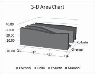
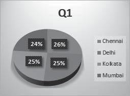
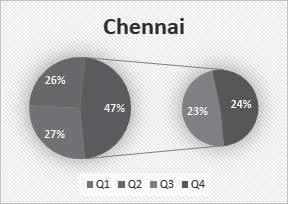
262 Office automation-ms-excel Line Charts Pie Charts Fig Line Charts Fig Pie Charts 444 INFORMATION TECHNOLOGY

263 Dashboard Reporting using Excel Bar Charts Fig Bar Charts 9.5 SELECTING THE APPROPRIATE CHART TYPE In order to display the data using a chart in dashboard, we need to first identify the purpose of the chart. Once we have clarity on what we want to represent by a chart, we can select the best chart type that depicts our message. Following are some suggestions on selecting a chart type If we want to compare data values, we can choose a bar chart, pie chart, line chart, or scatter chart. If we want to show distribution, we can do so with a column chart, scatter chart or line chart. If we want to show trends over time, we can use a line chart. If we want to represent parts of a whole, a pie chart can be an option. But, while we use a pie chart, remember that only two to three different data points with very different data values can be effectively depicted with the varying sizes of the Pie slices. If we try to depict more number of data points in a Pie chart, it can be difficult to derive the comparison. We can use Scatter chart in following scenarios We want to show similarities between large sets of data instead of differences between data points. We want to compare many data points without regard to time. The more data that we include in a Scatter chart, the better the comparisons we can make. INFORMATION TECHNOLOGY 445

264 Office automation-ms-excel 2010 In Excel 2013 and Excel 2016, a new feature Recommended Charts has been added, which helps to find a chart type that is suitable to current data. Once we can create a chart with a chart type, if required we can modify it later any time easily using the option of Change Charge Type in Design Tab. If we have data in a single Excel table, we can summarize the data in the way that is required using Excel PivotTables. Similarly, we can use PowerPivot feature. in Excel 2010, we have to install PowerPivot as an add-in, which is available on Microsoft site. One we activate the PowerPivot add-in, we will be able to see a PowerPivot Tab. (Note: We will get to know more about Power PivotTable and other Excel power tools such as Power PivotChart in other chapters.) PivotTables, Power PivotTables and Power PivotCharts come handy to display summarized results from big data sets on dashboard. It is advisable to get mastery on the normal PivotTable before we venture into the power tools. 9.6 CREATING A PIVOTTABLE We can create a PivotTable either from a range of data or from an Excel table. It is to be ensured that the table contains a header. No pivot can be made without a header/title. We can start with an empty PivotTable and construct it from scratch or make use of Excel Recommended PivotTables command (feature of Excel 2013) to preview the possible customized PivotTables for our data and choose one that suits our purpose. Consider the following data range that contains monthly average normal temperature for 4 places (Chennai, Delhi, Kolkata and Mumbai) as shown in Fig INFORMATION TECHNOLOGY

265 Dashboard Reporting using Excel Fig Data range for 4 Places To create a PivotTable from above data range, we do the following Ensure that in the table, the first row has headers. The headers will be the field names in the PivotTable. For making a PivotTable, either select entire table or just click on any cell in database Then click on the INSERT tab and select option PivotTable in the Tables group. Create PivotTable dialog box appears as shown in Fig INFORMATION TECHNOLOGY 447

266 Office automation-ms-excel 2010 Fig Creating PivotTable In Create PivotTable dialog box, under Choose the data that you want to analyze, we can either select a Table or Range from the current workbook or use an external data source. Hence, we can use the same steps to create a PivotTable form either a Range or Table. Choose default commands like New Worksheet. Data Range will be taken for entire table automatically. Click the OK button. A new worksheet will get inserted into our workbook on the left side of data sheet. The new worksheet contains an empty PivotTable. When we are inside the PivotTable, we can see PivotTable Field List on right hand side of screen and 2 new tabs i.e. Options and Design. (In Excel 2013 & 2016, instead of Options Tab, we can see Analyze Tab). Name the worksheet MyPivotTable using the Options Tab 448 INFORMATION TECHNOLOGY

267 Dashboard Reporting using Excel Fig PivotTable Field List The PivotTable Fields list contains the header names of the columns in the data range. We need to select PivotTable fields based on what data we want to display. By placing the fields in appropriate areas i.e. Filters, Rows, Columns and Values, we can obtain the desired layout for the data. For example, for calculating Quarterly average normal temperature for different cities, we need to do the following Click on the field Place in the PivotTable Fields list and drag it to ROWS area. Click on the field Qtr in the PivotTable Fields list and drag that also to Column area. Click on Normal Temperature and drag it to VALUES area. Also change the field setting to Average from Value field settings option. INFORMATION TECHNOLOGY 449

268 Office automation-ms-excel 2010 Fig PivotTable for calculating Quarterly average normal temperature The PivotTable is ready. If required, we can change the layout of the PivotTable by just dragging the fields across the areas. We can select / deselect fields in the PivotTable Fields list to choose the data we want to display. In case we want to select multiple options in the field list, we can do the same using filter option. At the bottom of PivotTable Field List, there is option called as Defer Layout Update. If this option is not selected, then the results for all the changes done in PivotTable can be seen immediately and if Defer Layout Update option is selected, then the changes will be reflected only if we manually click on Update button on Right hand bottom side of PivotTable Field list. In Excel 2010 and onwards, in PivotTable, a new feature called as Slicer has been added. It works like a filter. For more details about Slicers, please refer to chapter on Multi-Dimensional Analysis of Data. 9.7 DASHBOARD - INITIAL PREPARATION The first step in building a dashboard is the initial preparation. Before making any dashboard, we need to answer the following questions Why do we need the dashboard? Is this dashboard for a specific task, like showing the status of a project, or does it need to achieve a broader goal, like measuring business performance? Understanding why we are building the dashboard will guide we in the design. 450 INFORMATION TECHNOLOGY

269 Dashboard Reporting using Excel What purpose the dashboard will serve? The dashboard should highlight only the data that adds value. We should understand the data that is required. Anything outside that is unnecessary. What is the source of data? We should understand from where the data comes. It can just be an Excel worksheet or it can be through data connections to Excel workbook from various dynamic data sources. Who is the audience for the dashboard? Is this for a manager, an executive, a stakeholder, an external vendor or general audience? Understand their requirements and preferences such as how much time do they have to look at the dashboard, the level of detail they expect and how they would like to digest the information. For example, while choosing a chart type, knowing the audience helps we to decide on whether we have to show relations between values or we have to draw a specific comparison. Does the dashboard need to be static or dynamic? Can the dashboard be updated periodically, say, weekly or monthly, or does it require to get updated to continuously streamline the data changes that happen at the backend? This choice will change the way we build the dashboard. Does the dashboard need to be just a display or is it to be interactive? Can the dashboard have read-only access or do we have to provide interactive controls / features that enable certain people to explore the data as required? This choice also will change the way we build the dashboard. Once we have answers to these questions, decide on what Excel features we need and we don t need. This is because our goal and expertise is to produce an effective dashboard that suits the purpose. Next, identify the components of the dashboard. These can be text, tables, charts, interactive controls, etc. Decide on the dashboard layout with these components. Mockup Excel dashboard on a PowerPoint slide. Draw boxes for each component to get a sense of the layout and add quick sketches of the components that we want to include. We can also do this on a piece of paper. Get approval for this mockup from the management and/or the key audience before starting work on the actual dashboard. This will save time on rework. However, it is quite possible that we might have to tweak in some changes to the dashboard as the dashboard gets into usage and we receive feedback. But, the approved dashboard mockup is a really good starting for our work. 9.8 PREPARE THE DATA FOR THE EXCEL DASHBOARD Based on the choices we have, i.e. the answers we have for the questions in the Initial Preparation step, we need to prepare the data for the Excel dashboard. The data can be any of the following Results from data analysis Results from data exploration Data resulting from computations on the input data Data summarization from PivotTables or PowerPivot Tables INFORMATION TECHNOLOGY 451

270 Office automation-ms-excel SELECT THE DASHBOARD COMPONENTS In the above paras, we have learnt about various Excel features that we can use in a dashboard. Based on our requirements for the dashboard at hand, we can select any of the following Excel features for the dashboard components: Tables Sparklines Conditional Formatting. Charts Slicers Interactive Controls PivotTables PivotCharts We need to identify the static and dynamic components and also the components that are to be grouped for Slicers, if any. These components will help to align the required dashboard layout BUILD THE DASHBOARD This is the crucial and final step in creating a dashboard. This step involves assembling various dashboard components that we can efficiently and effectively use for dashboard preparation. Once the dashboard components are assembled, give it a final touch - Give a title to the dashboard. Incorporate a timestamp. Include the copyright information, if required. There is no universal rule or layout for a dashboard apart from some commonality. It all depends on our requirements and our goal should be to produce an effective dashboard for end user. Now we will learn how to use these steps for creating a dashboard based on some examples EXAMPLE EXECUTIVE DASHBOARD Now we will learn how to prepare a sample Executive dashboard. We need to remember that this dashboard can vary from company to company based on the requirements and preferences. Executive dashboards normally focus on the Business Performance, Revenue, Cost, Profits, Products, etc. Hence, Executive dashboards essentially display the KPIs. The visual impact necessary in this case would be to provide results at a glance, with not much detail as the executives will not normally have much time to dwell into the specifics unless it is absolutely necessary. An executive can be a head of the company or head of a specific department in a large company. The head of a company can be a CEO (Chief Executive Officer) or a MD (Managing Director). The executive would be mostly interested at a brief of the performance of the company as a whole. 452 INFORMATION TECHNOLOGY

271 Dashboard Reporting using Excel Let s take an example of a sample Company which deals in trading of FMCG products. There are various salespersons who deal in various household items. For each product, we have Sales, Price as well as Cost. Say our dummy data is like this. Fig Example of Data In our dashboard, we want to show following 4 reports - Revenue by Product Revenue by Sales Person Revenue price Ageing with count of transactions Revenue V/s Cost Month wise So we will create 4 Pivot tables for this in separate sheets or in a single sheet. The sample Pivots will be like this. INFORMATION TECHNOLOGY 453

272 Office automation-ms-excel 2010 The 1 st Chart is Product wise sale. The 2 nd one is Salesperson wise sale as shown in Fig Fig st Chart is Product wise Sale & 2nd Chart Salesperson wise Sale In 3 rd Chart, we are taking ageing of Revenue with a grouping of 30 to know in each pricing band how many items were sold. For this once we bring Revenue filed in Row Area, Right click any cell and Select Group and in Group by give 30 as shown in Fig INFORMATION TECHNOLOGY

273 Dashboard Reporting using Excel Fig rd Chart is Revenue with a grouping of 30 Like 3 rd PivotTable, in 4 th one we have grouped dates as Year and Month. Then in column area, we have taken revenue and cost both for a monthly comparison. INFORMATION TECHNOLOGY 455

274 Office automation-ms-excel 2010 Fig th Chart is grouped of dates as Year and Month Now we have created a Chart for each pivot table. We have made 2 Bar charts and 2 column Chart for each pivot table like this. Fig Bar Charts 456 INFORMATION TECHNOLOGY

275 Dashboard Reporting using Excel Fig Column Charts Now Cut all these charts and take to a new single sheet in such a way that all fits in single window. Also click any of the Pivot and insert slicer of Product and Salesperson as discussed earlier. Take slicer also to your dashboard sheet where all charts we have taken. Now right click each slicer and link with all the PivotTables as shown in Fig Fig Linking of Slicer with PivotTable And now our beautiful single page interactive dashboard is ready as shown in Fig INFORMATION TECHNOLOGY 457

276 Office automation-ms-excel 2010 Fig Single page interactive Dashboard Now we can play with slicers and try to change product/salesman. We may select single item or multiple items while pressing ctrl key. In the Fig , we have selected few items from the product and sales man slicer. Fig Dashboard 9.12 TEST, SAMPLE, AND ENHANCE THE DASHBOARD We need to test our dashboard to ensure that it displays the data accurately. Test it in various possible scenarios. Test for the precise updates (static or dynamic as is the case). 458 INFORMATION TECHNOLOGY