SIMCENTER 12 ACOUSTICS Beta

Size: px

Start display at page:

Download "SIMCENTER 12 ACOUSTICS Beta"

Maximilian Haynes
5 years ago
Views:

1 SIMCENTER 12 ACOUSTICS Beta 1/80

2 Contents FEM Fluid Tutorial Compressor Sound Radiation Import Structural Mesh Create an Acoustic Mesh Load Recipe Vibro-Acoustic Response Analysis Post-Processing Indirect BEM Acoustic Response of a Microphone Port Define Acoustic Model Define Microphone Meshes Acoustic Response Model Checking Post-Processing Page SC12 Beta Siemens PLM Software

3 The aim of this exercise is to show you how to create an acoustic mesh from the existing structural mesh, define the AML (Automatically Extruding Perfectly Matched Layer) feature and calculate the sound radiation from a compressor using a load recipe. You will also learn how to post-process the results at the end of this analysis. Simcenter FEM Acoustics NX Nastran - Vibro-Acoustic Response of a Compressor Page SC12 Beta Siemens PLM Software

FEM Fluid Tutorial Compressor Sound Radiation The aim of this exercise is to show you how to create an acoustic mesh from the existing structural mesh, define the AML (Automatically Extruding

4 FEM Fluid Tutorial Compressor Sound Radiation The aim of this exercise is to show you how to create an acoustic mesh from the existing structural mesh, define the AML (Automatically Extruding Perfectly Matched Layer) feature and calculate the sound radiation from a compressor using a load recipe. You will also learn how to post-process the results at the end of this analysis. The complete analysis sequence consists of the following steps: 1. Import Structural Mesh 2. Create an Acoustic Mesh 3. Load Recipe 4. Vibro-Acoustic Response Analysis 5. Post Processing Each of these steps is described in detail on the following sections Prerequisites Simcenter version 12 (beta) and the following files are required for this example: Compressor_Structure.bdf (Compressor Structural mesh Nastran file) Structural_velocity.unv (IDEAS universal file for the structural velocities) Page SC12 Beta Siemens PLM Software

bdf and expand the General Options, uncheck the option Create new solution for imported data.

5 1. Import Structural Mesh First of all, select the right module for the analysis: Go to File Import Simulation NX Nastran. Set the Input File Units to (N)(m)(kg), select the input file Compressor_Structure.bdf and expand the General Options, uncheck the option Create new solution for imported data. Click OK Save the Simulation file (Compressor_Structure_s.sim) and FEM files (Compressor_Structure_f.fem) at the desired locations and click OK You will get a report with the information on the imported mesh: Page SC12 Beta Siemens PLM Software

6 This report (Compressor_Structure.lis) is saved in your working directory. The structural mesh along with materials and properties are now imported. Page SC12 Beta Siemens PLM Software

Currently, the Compressor_Structure_s.sim is the displayed and work part.

7 2. Create an Acoustic Mesh Next, we need to create a layer of thin acoustic mesh (air) outside the structural mesh. We can also mesh inside the cavity if necessary, in this exercise; we are only interested in the radiated noise, and therefore, cavity mesh is not required. Currently, the Compressor_Structure_s.sim is the displayed and work part. To create an acoustic mesh from the existing structural mesh, we need to make the Compressor_Structure_f.fem as the work part. Right click on the Compressor_Structure_f.fem and select Make Work Part. The tabs and manuals in the ribbon bar are now changed accordingly. Page SC12 Beta Siemens PLM Software

This step allows you to add/create acoustic elements to the FEM model later.

8 Right click on the Compressor_Structure_f.fem and select the Edit and select Vibro-Acoustic as Analysis Type. This step allows you to add/create acoustic elements to the FEM model later. Select the tab Nodes and Elements and the command Convex Mesh (under the group Elements). Page SC12 Beta Siemens PLM Software

Make a rectangular trap to select all elements as input (or shortcut keys CTRL+A to select all), type the keyword SizeForAcoustics(3000) for the Element Size (this will create a convex mesh with

9 Make a rectangular trap to select all elements as input (or shortcut keys CTRL+A to select all), type the keyword SizeForAcoustics(3000) for the Element Size (this will create a convex mesh with element size good up to 3000 Hz). Offset Distance decides the size of the convex mesh. Assign 10 mm for the offset so the generated convex mesh is offset 10mm from the structural mesh. Toggle on Infinite Plane and select ZC plane, the Z infinite Plane is -50 (mm) from the bottom of the structural mesh. Make sure you select Create Plane to add this plane to the list. Create a new mesh collector and change the name to Convex mesh. Create the Show Result to preview the mesh. Create OK to close the dialog Box. The collector Convex Mesh is now added under the node 2D Collectors. Page SC12 Beta Siemens PLM Software

10 The convex mesh should be slightly larger than the structural mesh so that the number of elements for the air can be kept to minimum. Theoretical, we just need to define one layer of air outside the structural mesh. Please note that the Convex mesh is Not Exported to Solver by default. Next, we should create a solid mesh between the structural mesh and the convex mesh. However, instead of using the existing structural mesh (which is too fine a mesh), we can create a coarsening mesh (a wrapper mesh) for the structural mesh (this step is optional), and use this wrapper mesh and the convex mesh to create a solid mesh. Uncheck the Convex Mesh to hide this mesh for now Select the tab Surface Wrap and command Surface Wrap Recipe. Make a rectangular trap (or CTRL+A) to select all displayed elements, pick the option Wrap around the exterior, type the keyword SizeForAcoustics(3000) for the Element Size (this will create a wrapper mesh with element size good up to 3000 Hz). Assign 60 deg for Feature Angle. 2D Mesh for Output Option, Create a new mesh collector and change the name to Wrapper Mesh. Click on Apply and Cancel to close the dialog box Page SC12 Beta Siemens PLM Software

11 Page SC12 Beta Siemens PLM Software

The elements of this mesh is now added to the collector Wrapper Mesh You could see that the wrapper mesh does not capture the elements in the

12 A collector Wrapper Mesh and a Surface Wrap Recipes are now added to the tree. The Surface_Wrap_Recipe1 is still waiting to be updated. Right click on the Surface_Wrap_Recipe1 and select Wrap to create a wrapper mesh. The elements of this mesh is now added to the collector Wrapper Mesh You could see that the wrapper mesh does not capture the elements in the junction (i.e. PSHELL5) very well. We could define a local constraint to refine the elements in this area Uncheck the Wrapper Mesh and Check only the elements in collector PSHELL5 Page SC12 Beta Siemens PLM Software

Apply and Cancel Right click on the Surface_Wrap_Recipe1 and select Update to refine the existing wrapper mesh Select the tab Home and command Solid from Shell Mesh

13 Right click on the Constraints of the Surface Wrap Recipes, select the option New Local Resolution Constraint. Select option Size on Elements and select all displayed elements (CTRL+A), and then pick Local Subdivision level 3. Apply and Cancel Right click on the Surface_Wrap_Recipe1 and select Update to refine the existing wrapper mesh Select the tab Home and command Solid from Shell Mesh (under the group Mesh). Pick both (use the Ctrl key) 2d_convex_mesh and surface_wrap_shell meshes as the input, change the mesh type to CTETRA(4) Acoustic Fluid. Reduce Element Growth Rate to zero. Click Apply and Cancel Page SC12 Beta Siemens PLM Software

Display Internal Element Edges Select the shortcut keys CTRL+H (or tab View and

14 The 3d_mesh_from Shells is now added to the 3D Collectors. Right click on the Acoustic Fluid(1) and select Edit Display and toggle on the Display Internal Element Edges Select the shortcut keys CTRL+H (or tab View and command Edit Section) to see the interior of the mesh Page SC12 Beta Siemens PLM Software

Please note that by default, the status of both

15 Please note that by default, the status of both 2d_convex_mesh and surface_wrap_shell meshes are listed as Not exported to solver. This means both of these meshes will not be used in the calculation. These two meshes are created to generate the acoustic mesh 3d_mesh_from_shell. Right click on the collector Acoustic Fluid(1) and select Edit, pick the Edit button and then Choose Material Page SC12 Beta Siemens PLM Software

Select the Create Material button at the bottom, Select NX Nastran Mat10, and define 1.225 kg/m^3 for Mass Density and 340 m/s for Speed of Sound.

16 Select the Create Material button at the bottom, Select NX Nastran Mat10, and define kg/m^3 for Mass Density and 340 m/s for Speed of Sound. Click OK to close all dialog boxes Next, create a spherical field point mesh to recovery acoustic pressures and radiated power. Select tab Nodes and Elements, and command Sphere (under the group Elements). Select the option Automatic Sphere Position and Radius to define the primitive parameters. Change the Offset Z to m, Radius to 300 mm and type in the keyword SizeforAcoustics(3000) to estimate the element size good up to 3000 Hz (which is mm). Apply and Cancel Page SC12 Beta Siemens PLM Software

and select the Sphere Mesh Primitive as input, click

17 The Sphere Mesh Primitive is now added to the tree: Use shortcut keys CTRL+J (to change object display) and select the Sphere Mesh Primitive as input, click OK Page SC12 Beta Siemens PLM Software

Only display the Sphere Mesh Primitive, select tab Nodes and Elements and then Delete (under the group Elements), use the

18 Change the color to yellow and increase the Translucency and OK An infinite plane (Z plane) is defined at the bottom of the acoustic mesh, we will delete the lower part of the Sphere Mesh Primitive. Only display the Sphere Mesh Primitive, select tab Nodes and Elements and then Delete (under the group Elements), use the Lasso option to select a trap for the elements in the lower part of the sphere. Toggle on the Delate Orphan Nodes, Click OK Page SC12 Beta Siemens PLM Software

Now we are done with defining all the meshes in

fem and select Displace Simulation and then

This changes the tabs/groups and the commands.

19 Now we are done with defining all the meshes in FEM model, next step is to setup the simulation for vibroacoustic analysis. Right click on the Compressor_Structure_f.fem and select Displace Simulation and then Compressor_Structure_s.sim. This changes the tabs/groups and the commands. The acoustic Mesh and the Sphere Mesh Primitive are now greyed out. Page SC12 Beta Siemens PLM Software

3. Load Recipe The structural response already calculated and saved in a universal file. We will import this universal file using the load recipe command.

20 3. Load Recipe The structural response already calculated and saved in a universal file. We will import this universal file using the load recipe command. The load recipe will automatically create and attach the loads (frequency dependent velocities) to the structural mesh. Display only the structural mesh, right click on the Group and select New Group. Use the shortcut keys CTRL+A to select all displayed structural elements as input for this Group. Change the group name to Structural mesh Select the tab Home and command Load Recipes (under group Properties). Change the Data Type to Frequency Spectra and then select the Create button Browse for the data source and select the punch file Structural_velocity.unv. Select Retrieve information button to see the file contents in the universal file. Page SC12 Beta Siemens PLM Software

the Load Conditions tab; this lists the various loads conditions available in the source file: here we have only one load condition Select the Mapping

21 The punch file contains 250 spatial results (i.e. vector format) at 250 frequencies. Select the Autofill Options to automatically populate the Mapping table (map the mesh IDs defined in the punch file to the structural mesh IDs) Select the Load Conditions tab; this lists the various loads conditions available in the source file: here we have only one load condition Select the Mapping tab; the load recipe has automatically detected the Enforced velocities to be attached to the corresponding nodes in the.fem document. Click on the Run Validation Check Page SC12 Beta Siemens PLM Software

fem contains also acoustic mesh and the microphone mesh.

22 You should see that load is missing for the 33 % of the FEM model. This is OK as the fem Compressor_Structure_f.fem contains also acoustic mesh and the microphone mesh. We could limit the mapping to the structural mesh only: Page SC12 Beta Siemens PLM Software

23 Change the type to Group and pick the group Structural Mesh as target, click on the Run Validation Check again to confirm the mapping is OK this time. Click OK and Close to add this Load Recipe 1 to the Load Recipe Container Page SC12 Beta Siemens PLM Software

24 4. Vibro-Acoustic Response Analysis Right click on the Load Recipe 1 and select New Solution from Load Recipe. Select NX Nastran as Solver, Vibro-Acoustic as Analysis Type, and SOL 108 Direct Frequency Response as Solution Type, and Aggregated (i.e. Vector format) for the Hierarchy type In the Case Control, Edit the Output Requests. Click on Disable All first, then Enable to output the Acoustic Intensity, Acoustic Particle Velocity, Acoustic Power, and Acoustic Pressure. Click OK to close all dialog boxes Page SC12 Beta Siemens PLM Software

In the Bulk Data, for the Fluid-Structure Interface Modeling

the Effect of Structure on Fluid Only (Weak) to define a one

Accept the default settings for the Fluid Interface (FSET) and

25 In the Bulk Data, for the Fluid-Structure Interface Modeling parameters, select the Create Modelling Object button, select the Effect of Structure on Fluid Only (Weak) to define a one way coupling. Accept the default settings for the Fluid Interface (FSET) and Structural Interface (SSET). Click OK to close all dialog boxes Page SC12 Beta Siemens PLM Software

Objects (under Solution 1 from Load Recipe 1) and select New Simulation Object, and then Automatically

26 An Enforced Velocities (under the Load Container) and a Solution 1 from Load Recipe 1 is created on the tree Toggle on the 3D collector to display the acoustical mesh Right click on the Simulation Objects (under Solution 1 from Load Recipe 1) and select New Simulation Object, and then Automatically Matched Layer. Select Create Region icon for the Automatically Page SC12 Beta Siemens PLM Software

Click OK Similarly, Select Create Region Icon for the Infinite Plane 1, pick any element face on the bottom using the

27 Matched Layer Surface, pick any element face on the surface (not on the bottom) using the method Feature Angle Element Faces (with Feature Angle 30 Deg). Click OK Similarly, Select Create Region Icon for the Infinite Plane 1, pick any element face on the bottom using the method Feature Angle Element Faces (with Feature Angle 30 Deg). The Type should set to Rigid Plane (symmetry, Zero Velocity). Click OK to close all dialog boxes Page SC12 Beta Siemens PLM Software

28 This Automatically Matched Layer(1) with Rigid Plane is now added to the Solution 1 from Load Recipe1. Right click on the Data Source 1 and click on the Creating Forcing Frequencies button Page SC12 Beta Siemens PLM Software

Click OK Make sure you Add the defined Forcing frequencies to the list.

29 Select the Create button, and then option Linear Sweep (FREQ1), Step Value, Start Frequency from 10 Hz to 2500 Hz, step value of 10 Hz. Click OK Make sure you Add the defined Forcing frequencies to the list. Click on Close and OK Save the model Right click on the Solution 1 from Load Recipe 1 and select Model Setup Check and make sure you do not have any error Page SC12 Beta Siemens PLM Software

30 Right click on the Solution 1 from Load Recipe 1 and select Solve and OK to launch the job. This will take a few minutes to export the input files. Page SC12 Beta Siemens PLM Software

31 And another 10 minutes to finish the job. Page SC12 Beta Siemens PLM Software

Results and then the Create Scenario button.

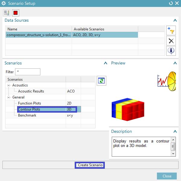
32 5. Post-Processing To quickly review the results: Right click on the Vibro-Acoustic (under Results) and select Post-Processing Scenario Select first the Acoustic Results and then the Create Scenario button. This will bring you the acoustic radiated power plot in the current view port Page SC12 Beta Siemens PLM Software

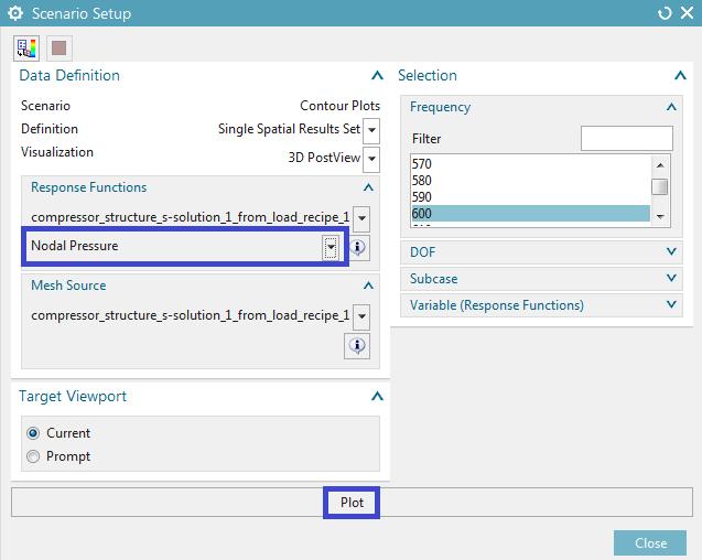
33 The Results tab is now active. Pick the icon Editing (under group XY Graph) and double click on the label Power (on the Y-axis), change the Axis type to db and accept the rest default settings and OK. Select the Scenario Setup (under group Tools) and pick the Contour Plots and then the Create Scenario button. Select the Nodal Pressure as the response Function and frequency at 600 Hz. Click on the Plot button to see sound pressure levels on both microphone mesh and acoustical mesh Page SC12 Beta Siemens PLM Software

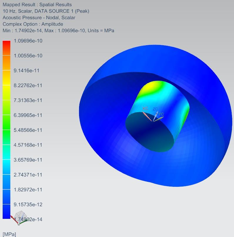
34 Page SC12 Beta Siemens PLM Software

Select the icon Edit Post View (under group Post View) and toggle on the option Applying db Scaling to display the pressure in db scale Select the Scenario Setup (under group Tools) again and pick

35 Select the icon Edit Post View (under group Post View) and toggle on the option Applying db Scaling to display the pressure in db scale Select the Scenario Setup (under group Tools) again and pick the Contour Plots and then the Create Scenario button. Select the Nodal Acoustic Intensity as the response function and frequency at 600 Hz. Toggle on option Magnitude. Click on the Plot button to see the intensity on the microphone mesh Page SC12 Beta Siemens PLM Software

36 Similarly, display the Nodal Acoustic Velocity (Magnitude) at 600 Hz Page SC12 Beta Siemens PLM Software

Select the Post Processing Navigator from the left border bar, right click on the Vibro Acoustic and select Load to load results for all

37 Instead of post-process results in Simulation Navigator, users could also post-process the results in Post- Processing Navigator, which provides more tools and options. Select the Post Processing Navigator from the left border bar, right click on the Vibro Acoustic and select Load to load results for all frequencies Expand the results under Forcing Frequency 60, 600 Hz, and double click on the Scalar from the Pressure Nodal. This display the pressure field on both microphone mesh and acoustic mesh at 600 Hz Page SC12 Beta Siemens PLM Software

38 To see only the pressures on the microphone mesh, toggle off the 3D Elements from the Viewports Page SC12 Beta Siemens PLM Software

This display can be saved in the Simulation

the simulation navigator Go back to Post Processing

39 This display can be saved in the Simulation Navigator; select the icon Save State (under the group Layout), assign a name to this display and OK. Now this display is added to the Layout States in the simulation navigator Go back to Post Processing Navigator Page SC12 Beta Siemens PLM Software

To see how sound pressure level at one microphone changes with frequencies, select the icon Create Graph (under the group Tools), Change the type to Across Iterations, X Axis display is Frequency

40 To see how sound pressure level at one microphone changes with frequencies, select the icon Create Graph (under the group Tools), Change the type to Across Iterations, X Axis display is Frequency (from 10 Hz to 2500 Hz, with 1 step). Manually pick any node (microphone) from the model and Apply to see the XY plot of the pressure at this microphone Pick the Create New Window to display this XY plot in a new window Page SC12 Beta Siemens PLM Software

This graph is added to collector under the Vibro Acoustic.

Select the icon Edit Post View (under group Post View) and second tab Display.

toggle on the option Applying db Scaling to display the pressure in db scale Select third tab

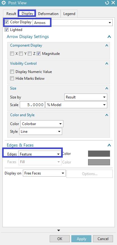
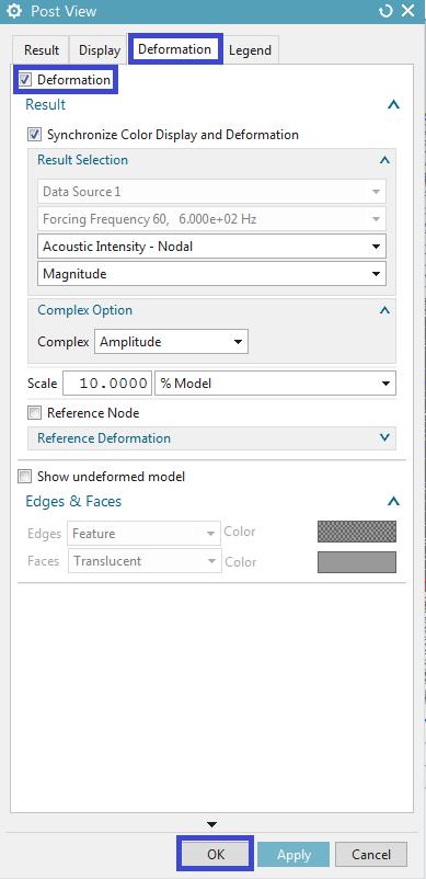
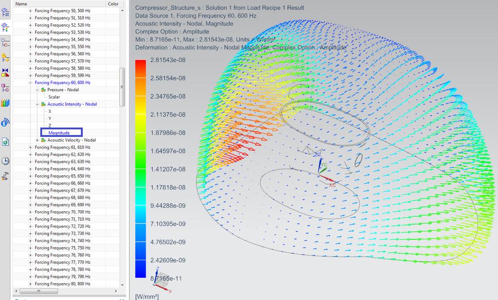
41 This graph is added to collector under the Vibro Acoustic. Double click on the Magnitude (under the Acoustic Intensity Nodal at 600 Hz). Select the icon Edit Post View (under group Post View) and second tab Display. Select Arrows for the Color Display and Feature for the Edges. toggle on the option Applying db Scaling to display the pressure in db scale Select third tab Deformation and toggle on the option Deformation, select OK to display the Acoustic intensity on the deformed microphone mesh with arrows Page SC12 Beta Siemens PLM Software

42 Page SC12 Beta Siemens PLM Software

43 We could overlay two contour plots. For example, overlay the existing Acoustic Intensity plot with the Pressure Nodal scalar plot at the same frequency: Right click on the Scalar (under the Pressure Nodal at 600 Hz) and select Overlay. Now two plots are superimposed. Toggle off the 2D Elements from the second Post View so that pressures are only displayed on the 3D Elements Please note that only one legend can be the master. For now, the second post view (for pressure) is the master view. To display acoustic intensity legend for these two superimpose plots, just active the first Post View (for intensity): Click on the first Post View to display the legend just for acoustic intensity Page SC12 Beta Siemens PLM Software

44 Page SC12 Beta Siemens PLM Software

45 Page SC12 Beta Siemens PLM Software

46 In this tutorial, a pure acoustic analysis is considered. A microphone port is excited by a monopole located outside the port. Three acoustic microphone meshes are defined to capture the acoustic response inside and outside the port. Users will learn how to import an acoustic mesh and define field point meshes, setup a perforated panel using Rigid Transfer Relation admittance, and postprocess the results. Simcenter BEM Acoustics Indirect BEM - Acoustic Response of a Microphone Port Page SC12 Beta Siemens PLM Software

Indirect BEM Acoustic Response of a Microphone Port The complete analysis sequence consists of the following steps: 1. Define Acoustic Mesh 2. Define Microphone Meshes 3. Acoustic Response 4.

47 Indirect BEM Acoustic Response of a Microphone Port The complete analysis sequence consists of the following steps: 1. Define Acoustic Mesh 2. Define Microphone Meshes 3. Acoustic Response 4. Model Checking 5. Post-Processing Each of these steps is described in detail on the following sections Prerequisites Simcenter version 12 (beta) and the following files are required for this example: MicrophonePort.bdf: Acoustic mesh in Nastran Bulk Data file format SoundPower.txt: Acoustic power of sound source in text file format Beta.txt: Transfer relation admittance in text file format Page SC12 Beta Siemens PLM Software

1. Define Acoustic Model File Import Simulation and select to import a NX Nastran file. Click OK Choose the Nastran BDF Files (*.bdf) file type from the pull-down menu and select the MicrophonePort.

48 1. Define Acoustic Model File Import Simulation and select to import a NX Nastran file. Click OK Choose the Nastran BDF Files (*.bdf) file type from the pull-down menu and select the MicrophonePort.bdf file. Set the input file units to (mn)(mm)(kg). Expand General Options, toggle off the option Create new solution for imported data. Click OK to import Page SC12 Beta Siemens PLM Software

49 Save both simulation and FEM files (*.sim and *.fem) to the desired folders and OK Page SC12 Beta Siemens PLM Software

The imported mesh is a structural mesh, we will convert the structural mesh to an acoustic mesh, and therefore the missing property cards for the structural

50 Two warnings and errors are found from importing this model. The errors are due to missing property cards for the shell elements. We could ignore these warnings and errors as the missing information are not relevant to the acoustic model. The imported mesh is a structural mesh, we will convert the structural mesh to an acoustic mesh, and therefore the missing property cards for the structural mesh are not important. Close the information box and Save the Sim and Fem files Right click on the MicrophonePort_f.fem and select Make Displayed Part This changes the commands in the ribbon bar. Page SC12 Beta Siemens PLM Software

Indirect Acoustic. Click OK The mesh is greyed out.

labelled with -1), which could not be used in the acoustic analysis.

Select the tab Nodes and Elements and command Modify Type (under group Elements), select all

51 Right click on the MicrophonePort_f.fem and select Edit, change the Solver to Simcenter Acoustics BEM, and Analysis Type to Indirect Acoustic. Click OK The mesh is greyed out. This is because a structural mesh was imported (the 7 th field of the cards GRID are not labelled with -1), which could not be used in the acoustic analysis. Therefore, the mesh type needs to be changed. Select the tab Nodes and Elements and command Modify Type (under group Elements), select all elements (using shortcut key CTRL+A) and change the element type to QUAD4 Acoustic and OK Now the color of the mesh changes back to the default green color. All elements (including triangular elements) are now suitable for acoustic analysis Page SC12 Beta Siemens PLM Software

Right click on the collector Acoustic Shell(1) and

the button Edit, and then Choose Material, and

the Simcenter Acoustic BEM MAT from the list,

52 Right click on the collector Acoustic Shell(1) and select Edit, for Acoustic Fluid Property, select the button Edit, and then Choose Material, and then Create Material (at lower right corner) Pick the Simcenter Acoustic BEM MAT from the list, define the following values for fluid Mass Density (RHO) and Speed of Sound (C). Click OK to close all dialog boxes Page SC12 Beta Siemens PLM Software

In many circumstances, we need to know the direction of the element normal

Right click on the acoustic mesh and select the Check and Element Normals.

Normals All element normals are pointing out, this means the outer surface of

53 In many circumstances, we need to know the direction of the element normal vectors to identify the positive and negative surfaces of the mesh. Right click on the acoustic mesh and select the Check and Element Normals. Select all elements (using shortcut key CTRL+A), and then click on the Display Normals All element normals are pointing out, this means the outer surface of the mesh is Top side, and inner surface is Bottom side. Page SC12 Beta Siemens PLM Software

54 2. Define Microphone Meshes We will define two microphone meshes, one inside and one outside the port. Select the tab Nodes and Elements and command Plane (under group Elements), select QUA4 Microphone as Type. Click on the button Automatic Plane Position and Size and change the plane location to (8.1, 0.39, 0.01), 3 mm on both side, 0.15 mm for Maximum Element Size. Automatic Creation the Destination Collector and toggle on Preview to see the microphone mesh. Click on Apply but do not hit Cancel, as we will define another plane mesh Again, click on the button Automatic Plane Position and Size and change the plane location to (8.285, 1.995, ), 1.73 mm and 0.83 mm on each side, mm for Maximum Element Size. Automatic Creation the Destination Collector and toggle on Preview to see the microphone mesh (hide the acoustic mesh first). Click on Apply and hit Cancel Page SC12 Beta Siemens PLM Software

the select objects and OK Change the acoustic mesh color to blue and

55 Make the acoustic mesh transparent so that we could see all meshes. Use shortcut key CTRL+J for the class selection, pick the acoustic mesh as the select objects and OK Change the acoustic mesh color to blue and increase the Translucency. Click OK Page SC12 Beta Siemens PLM Software

For indirect BEM acoustic calculation, acoustic pressure and velocity could only be recovered on the microphone mesh and not on the acoustic mesh.

56 For indirect BEM acoustic calculation, acoustic pressure and velocity could only be recovered on the microphone mesh and not on the acoustic mesh. In order to display the acoustic pressure on the acoustic mesh, we could replica the very same acoustic mesh as the microphone mesh: Toggle off both Microphone Surface(1) and Microphone Surface(2) Select the tab Nodes and Elements and command Translate (under group Elements), select Element Copy and Translate as Type. Use shortcut key CTRL+A to select all displayed acoustic elements. 0 mm distance for all 3 directions and OK Page SC12 Beta Siemens PLM Software

The new mesh is now added to the same acoustic collector.

group Elements), select the duplicated mesh and change the element type to QUA4 Microphone.

Click OK A new microphone mesh collector is now created for this microphone mesh.

57 The new mesh is now added to the same acoustic collector. We will change the mesh type next: Select the tab Nodes and Elements and command Modify Type (under group Elements), select the duplicated mesh and change the element type to QUA4 Microphone. Automatic Creation of Destination Collector. Click OK A new microphone mesh collector is now created for this microphone mesh. Show only the new microphone mesh, select the tab View, pick the Edit Section (under group Visibility), select the Y-plane and adjust the Offset to get the Y-section view of the mesh. Click OK Page SC12 Beta Siemens PLM Software

58 There is a partition in this microphone mesh, this creates a junction edge at the connected nodes. This will cause problems later as unique element normals could not be defined on the elements connected to the junction edge. We could either delete this partition from the microphone mesh or detach this partition from the rest of the mesh. Click OK to close the View Section dialog box. Select the tab Nodes and Elements, pick the Delete (under group Elements), use the option Feature Angle Elements (make sure Feature angle is 30 deg) and pick any element on the partition. This select all elements on the partition. Toggle on the option Delete Orphan Nodes and OK Page SC12 Beta Siemens PLM Software

Now there is no junction edges in this microphone mesh, but the junction edge is still in the acoustic mesh. Sysnoise will duplicate nodes along the junction edge (to detach the partition).

59 Now there is no junction edges in this microphone mesh, but the junction edge is still in the acoustic mesh. Sysnoise will duplicate nodes along the junction edge (to detach the partition). These duplicated nodes will coincide with some nodes of this microphone mesh and create errors in the calculation later. Therefore we need to move these coincident nodes on this microphone mesh slightly away from the junction edge in the acoustic mesh. Select the tab Nodes and Elements, pick the Translate (under group Nodes), Change the Method to scale Model, use the option Feature Edge Nodes (make sure Feature angle is 30 deg) and pick any node on the edges of the deleted partition. Change the Scale Factors for X and Y to and keep the scale factor for Z to 1. Click OK Page SC12 Beta Siemens PLM Software

60 Select the tab View, pick the Clip Section (under group Visibility) to see the full model again Page SC12 Beta Siemens PLM Software

The mesh is now greyed out, as we have now defined the simulation type yet. Right click on the MicrophonePort_s.sim and select New Simulation.

61 3. Acoustic Response Right click on the MicrophonePort_f.fem and select Display Simulation and MicrophonePort_s.sim This changes the commands on the ribbon bar, the tree so that you could now define necessary boundary conditions, loads and simulation objects for the analysis. The mesh is now greyed out, as we have now defined the simulation type yet. Right click on the MicrophonePort_s.sim and select New Simulation. Change the Name of the solution to Solution 1 Recover the results on the bottom side. Simcenter Acoustic BEM for the Solver, Indirect Acoustic for the Analysis Type, Acoustic Response for the Solution Type. Use Results of Acoustical Element from the Bottom side (i.e. to recover the pressure on the inner surface). Do not close this dialog box yet Page SC12 Beta Siemens PLM Software

Select the tab Acoustic Power, pick option Selected Groups of 2D Microphone Elements and then New Group and pick the smaller plane microphone mesh as input, so

62 Edit the Output Requests, toggle on Pressure, Velocity, Intensity to output these results in Vector (Sort1) format (i.e. contour plots). For Function (Sort2) Pressure, use the option Selected Microphone Nodes and arbitrary pick some nodes on both plane microphone meshes. Select the tab Acoustic Power, pick option Selected Groups of 2D Microphone Elements and then New Group and pick the smaller plane microphone mesh as input, so that acoustic power will be calculated on this mesh only. The power will be displayed in a XY plot (i.e. Function or Sort2 format). OK to close all dialog boxes Page SC12 Beta Siemens PLM Software

Note that for Indirect Acoustic analysis, if a microphone mesh is overlapped with the acoustic

velocity, intensity) on the inner side (I.e. Bottom side) of the Now the Solution 1 Recover the

63 Note that for Indirect Acoustic analysis, if a microphone mesh is overlapped with the acoustic mesh, we could request to calculate the results the microphone mesh based either side of the acoustic mesh. We select the bottom side, this mean the microphone mesh will recover the results (pressure, velocity, intensity) on the inner side (I.e. Bottom side) of the acoustic mesh. Now the Solution 1 Recover the results on the bottom side with a Subcase Acoustic Response 1 is added to the tree. We will define Load and Simulation Object to this solution. Page SC12 Beta Siemens PLM Software

Show only the acoustic mesh, select the tab View, pick the Edit Section (under group Visibility), select the Y-plane and adjust the Offset to get the Y-section view of the acoustic mesh.

64 Show only the acoustic mesh, select the tab View, pick the Edit Section (under group Visibility), select the Y-plane and adjust the Offset to get the Y-section view of the acoustic mesh. Click OK to close the dialog box There is a partition separates the port into two parts. By default the partition is rigid and not permeable, so sound cannot be transferred from one part to another. We could assume the partition is perforated and transmitted sound is allowed. The perforated partition can be represented by an acoustic property; namely the Transfer Admittance. Right click on the Simulation Object under the Solution 1, select New Simulation Object and then Transfer Admittance Use the option Feature Angle Elements (make sure feature angle is set to 30 deg) and pick any element on the partition. This selects all the elements on the partition. Change the Method to Rigid Transfer Admittance and input Format to Table Constructor. Select the option Import from Text File and pick the file Beta.txt and import. The data is now listed. Click OK to close this window only Page SC12 Beta Siemens PLM Software

65 Selected the option Plot(XY) to see the XY plot of the data and Create New Window for this plot. Click OK to close Page SC12 Beta Siemens PLM Software

Right click on the Loads under the Subcase and select New Load and then Acoustic Monopole Select the option Point Dialog to define the location of the

66 Select the tab View, pick the Clip Section (under group Visibility) to see the full model Next we will define a monopole sound source outside the microphone port. Right click on the Loads under the Subcase and select New Load and then Acoustic Monopole Select the option Point Dialog to define the location of the source at (15mm, 10mm, 10mm). and OK Select the Power as source type, unit in W and select the option Table. Pick option Import from Text File, pick the file SourcePower.txt and import. The data is now listed. Click OK to close this window only Page SC12 Beta Siemens PLM Software

67 Selected the option Plot(XY) to see the XY plot of the data and Create New Window for this plot. Click OK to close all dialog boxes Page SC12 Beta Siemens PLM Software

Right click on the Solution 1 - Recover the results on the

Select the Crate button and define frequencies using

68 Right click on the Solution 1 - Recover the results on the bottom side and Edit. Select the Create Forcing frequencies. Select the Crate button and define frequencies using Frequency Sweep, start from 3000 Hz, to Hz, step value 50 Hz. Click OK. Next Add the define frequency to the List and Close and OK Page SC12 Beta Siemens PLM Software

69 If not sound source powers are not defined at these forcing frequencies, program will interpolate data automatically. Save all the files Page SC12 Beta Siemens PLM Software

Right click on the Solution 1 - Recover the results on the bottom side and Model Setup check.

70 4. Model Checking It is advised to check on the model first and make necessary changes before submit the job, which could run for a long time. Right click on the Solution 1 - Recover the results on the bottom side and Model Setup check. Make sure no errors found Right click on the Solution 1 - Recover the results on the bottom side and select Solve. Pick the option Solve Model Quality Results and OK Page SC12 Beta Siemens PLM Software

Frequency Elemental) and toggle on all the meshes listed

71 Go to Post-Processing Navigator and right click on Acoustic and select Load Double click on the Scalar (under the Maximum Frequency Elemental) and toggle on all the meshes listed under the Viewports Page SC12 Beta Siemens PLM Software

This display shows that all meshes (acoustic and microphone meshes) are 100% good up to 164050 Hz. Which is much higher than the defined maximum forcing frequency at 15000 Hz.

72 This display shows that all meshes (acoustic and microphone meshes) are 100% good up to Hz. Which is much higher than the defined maximum forcing frequency at Hz. Double click on the Scalar (under the Free Edges Nodal) and toggle on only the acoustic mesh listed under the Viewports. This highlights the free edges detected in the acoustic mesh Similarly, double click on the Scalar (under the Junction Edges Nodal) and toggle on only the acoustic mesh listed under the Viewports. This highlights the junction edges in the acoustic mesh. Page SC12 Beta Siemens PLM Software

73 Page SC12 Beta Siemens PLM Software

74 When submitting the job, Sysnoise will automatically detect these edges and create duplicated nodes on the junction edges, add the appropriate boundary conditions to these free edges and junction edges. Go back to the Simulation Navigator and right click on the Solution 1 - Recover the results on the bottom side and select Solve. Pick the submit mode Solve, click on Edit Solver Parameters. Use 90% of System Memory and assign 4 processes (if available) to run this job. Click OK Click OK to run the job Page SC12 Beta Siemens PLM Software

75 Page SC12 Beta Siemens PLM Software

This will bring you the Microphone Pressure Frequency Spectra setup, select all 3 listed microphones and Plot

76 5. Post-Processing Right click on the Acoustic (under Results) and select Post-Processing Scenario Select first the Function Plots and then the Create Scenario button. This will bring you the Microphone Pressure Frequency Spectra setup, select all 3 listed microphones and Plot Select the icon Editing (under group XY Graph) and double click on the Y-axis Pressure(kpa) and change the Axis Type to db scale Page SC12 Beta Siemens PLM Software

77 Select the Scenario Setup (under group Tools) and pick the Function Plots again and then the Create Scenario button. Select the Microphone Acoustic Power Frequency Spectra and Plot Page SC12 Beta Siemens PLM Software

78 Select the Scenario Setup (under group Tools) and pick the Contour Plots and then the Create Scenario button. Nodal Pressure is now selected. Select frequency Hz and click on Plot Page SC12 Beta Siemens PLM Software

79 Select the icon Edit Post View (under group Post View) and toggle on the option Applying db Scaling to display the pressure in db scale Page SC12 Beta Siemens PLM Software

Select Nodal Acoustic Intensity at frequency 10700 Hz and toggle on

80 Select the Scenario Setup (under group Tools) and pick the Contour Plots and then the Create Scenario button. Select Nodal Acoustic Intensity at frequency Hz and toggle on Magnitude. Click on Plot. Just as before, change the display to db level. Page SC12 Beta Siemens PLM Software

CHAPTER 8 FINITE ELEMENT ANALYSIS

If you have any questions about this tutorial, feel free to contact Wenjin Tao (w.tao@mst.edu). CHAPTER 8 FINITE ELEMENT ANALYSIS Finite Element Analysis (FEA) is a practical application of the Finite