TatukGIS Editor/Viewer Viewer 1.6.4

Transcription

1 Viewer 1.6.4

2 All rights reserved. No parts of this work may be reproduced in any form or by any means - graphic, electronic, or mechanical, including photocopying, recording, taping, or information storage and retrieval systems - without the written permission of the publisher. Products that are referred to in this document may be either trademarks and/or registered trademarks of the respective owners. The publisher and the author make no claim to these trademarks. While every precaution has been taken in the preparation of this document, the publisher and the author assume no responsibility for errors or omissions, or for damages resulting from the use of information contained in this document or from the use of programs and source code that may accompany it. In no event shall the publisher and the author be liable for any loss of profit or any other commercial damage caused or alleged to have been caused directly or indirectly by this document. Printed:

3 Contents I Table of Contents 5 Part I Help 1 Introduction... 5 Product Introduction... 5 Product Specifications... 7 Contact Information... 8 Acknowledgments Menus... 9 File... 9 New Project... 9 Open Project Save Save Project As Save All Export to image Internet Server... Wizard 13 Print Print to PDF Print Preview Recent Files Exit Edit Undo Redo Copy Copy Special Clear Clipboard Save Clipboard Load Clipboard View Toolbars Panels Scale Selected Legend MiniMap Intro Search Data Minimap Desktops Themes Language Full screen Map Full Extent Layer Extent Selected Extent Zoom mode Zoom extended... mode 35 Drag mode Select mode I

4 II Localize Select by Point Select by Line Select by Polygon Select by Circle Select by Rectangle Select by Clipboard Deselect Clear Selection Invert Selection Select All Select Type Equality Disjoint Intersect Touch Cross Within Contains Overlap Map units Layer New Add Remove Import Export Merge Restructure Save layer properties Load layer properties Properties Move Up Move Down Visible Shape Edit modes Edit Point Multipoint Line Polygon Rectangle area Rectangle outline Rectangle rotated... area 68 Rectangle rotated... outline 69 Polygon90 area Polygon90 outline Circle area Circle outline Circle 3point area Circle 3point outline Line free Line Add Part Delete Part Delete Shape Revert Shape... 75

5 Contents III Change Winding Split shapes Union shapes Clipboard buffer Clipboard convexhull Line Smooth Data Export data Import data Set column value Tools Map hint Measure Map hotlinks Topology Options Help Tutorial Check for Updates About Part II Tutorial 1 Introduction... to the Viewer/Editor Tutorials 91 2 Tutorials Viewer Tutorial 1 - Main... Menu Controls/Options 91 Main Menu, MiniMap Data table, map... hints 94 Program Options... (Settings) 96 Layer Information Coordinate System... information 101 Scale Setting Tutorial 2 - Layer... Appearance Properties 102 Vector Layers Pixel Layers Use of Symbols Tutorial 3 - Thematic... Map Rendering 113 Set-up style definations Apply styles Color-Gradient... Value Theme 119 Rendering Based... on a Formula 122 Rendering Line... Widths 124 Rendering on Text... Information 128 Tutorial 4 - Thematic... Rendering Wizard 132 Tutorial 5 - Rendering... DTM Data 136 Tutorial 6 - Pie... and Bar Charts 140 Color-Gradient... Value Theme 140 Pie and Bar Charts Chart sizes Tutorial 7 - Label... Rendering 147 Label Styles Label Positions Polygon Label... Positions 158 Tutorial 8 - Spatial... Select 159 Select versus Localize Spatial Selection... Modes 162 Copy & Copy Special... to Clipboard Layer 167 III

6 IV Tutorial 9 - Attribute... Query 170 Tutorial 10 - Measurement... Tools 173 Tutorial 11- Export... to Image file 175 Tutorial 12 - Export... Image Mosaics 180 Tutorial 13 - Print,... Print Preview, PDF 184 Tutorial 14 - URL... Referencing 187 Editor Tutorial 1 - Main... Menu Controls 190 Tutorial 2 - Digitize... New Map Geometry 192 Create New Vector... Layer 192 Create Vector... Polyline Data 196 Create Vector... Polygon Data 203 Delete Vectors Custom Edit Modes Line/Polygon Smoothing Create Vectors... Using COGO 217 Tutorial 3 - Edit... Existing Map Data 224 Geometry Editing Attribute Editing... & Restructuring 226 Tutorial 4 - Unions... and Splitting 229 Unions of Shapes Splitting of Shapes Tutorial 5 - Export... Vector Layer/Clipping 236 Tutorial 6 - Layer... Merging 240 Tutorial 7 - Import... Attribute Data 244 Tutorial 8 - Buffers Topology Building... & Correcting 254 A Short Guide Tutorial FAQ... items 265 Index 267

7 Help 1 5 Help Enter topic text here. 1.1 Introduction Product Introduction Introduction to the TatukGIS Viewer & Editor Programs and Features The TatukGIS Viewer is a free software product which may be used free of charge and the TatukGIS Editor is a commercial software product requiring the purchase of a license. The Editor supports all features in the Viewer plus additional features mostly relating to the creation and editing of vector map information. The company TatukGIS ( is the owner of both the Viewer and Editor products. Both products are developed by TatukGIS from the TatukGIS Developer Kernel GIS toolkit product. Per the terms of the TatukGIS license agreement, the TatukGIS Viewer can be redistributed without charge under the condition that no changes are made to the application. A license to use the TatukGIS Editor can be purchased only from TatukGIS or by a TatukGIS authorized reseller. Refer to the TatukGIS software license agreement for more details. Two sources of documentation are provided for the Viewer and Editor products. 1. The Help files provide a brief description of the action performed or the feature called by each menu command in the program along with brief instructions on how to use each feature. The Help files can be accessed under the Help/Help menu. 2. The Tutorials demonstrate the use of many of the features supported by the Viewer and Editor products with real data sets. Both the Viewer and Editor products include the full set of tutorials for both the Viewer and the Editor. The Tutorials are organized into to sets. The first set, titled Viewer Tutorials, relates to features supported by both the Viewer and Editor. The second set, titled Editor Tutorials, relates to functionality supported only by the Editor. The Tutorials can be accessed under the Help/Tutorials menu. The Viewer and Editor products are updated from time to time, and the updates may be downloaded via the internet. Use the Help/Check for updates menu while connected to the internet to check for the availability of a new update. TatukGIS Viewer The free TatukGIS Viewer is designed to open and view GIS/CAD and raster image files and projects composed of these files. The Viewer reads most file formats and supports many custom rendering and other features. Map data in multiple file formats, e.g., SHP, DXF, TAB, GML, TIFF, MrSID, etc. can be opened as separate layers together as part of a single project, with no need to import the data to any common, internal data format. The Viewer can save project configurations to a TatukGIS project file. The free Viewer offers an easy way to evaluate TatukGIS technology and is a helpful companion tool for the TatukGIS Developer Kernel (DK) toolkit and Internet Server products. Any mapping project that can be visualized in the free Viewer can be exported to a TatukGIS project file which is compatible with other TatukGIS products or custom applications/solutions created from the TatukGIS Developer Kernel toolkit. Features of the Viewer: Open/read all TatukGIS supported vector and raster file formats, natively, with no importing to an internal format (see the Specifications for a listing of the formats) Open map layers in multiple formats together in the same project (work place) Open TatukGIS projects as well as most projects created with ESRI ArcView or MapInfo Professional products

8 6 Create new TatukGIS project files to save all configurations and settings that are unique to a project Zoom in/out, pan Unlimited number of layers Specify map scale for viewing/printing Add, remove, reorder, and turn on/off layers in a project via the Legend panel Alter the appearance (colors, styles, fills, boarders, outlines,symbols, transparency level,etc.) vector map layers Manipulate pixel layers, including transparency, histogram, brightness, color enhancing,etc. Generate custom thematic map presentations, including colored-gradient value themes, based on vector attribute values Color Render DTM/grid layer Present data as bar or pie charts Present attribute information as a table Use CGM, WMF, and TrueType symbols to represent points, lines, polygon fills and perimeters URL hot-linking of map objects to any document referenced by a valid URL (web page, file, even mailto) Custom render label appearances and positioning Attribute Queries using SQL Query Builder, based on either numeric or text information Spatial Queries (by point, line, circle, rectangle, polygon), Copy to clipboard layer Measurement tools for distance, area, and perimeter Print and print preview, print to PDF format Copy to Clipboard layer Copy visible extent of all layers to Windows clipboard with the EMF meta format Export visible or full extent to image files: JPEG, PNG, TIFF, BMP, or TatukGIS PixelStore, PDF Mosaic multiple geo-registered images and export to an image file R-tree spatial indexing to enhance performance with very large vector files Multi-language user interface (English, Spanish, German, French, Portuguese, Italian, Greek, Russian, Japanese...) The "Internet Server Wizard" to easily set up a simple ASP.NET projects for interactive web publishing of mapping projects with the TatukGIS Internet Server. An easy and affordable path to web publish any GIS project. TatukGIS Editor The Editor product supports all the functionality in the TatukGIS free Viewer, plus the additional features relating to the digitizing, editing, importing, exporting, merging, converting, and other manipulation of vector geometry and attributes as are listed below. The "Swiss pocket knife" nature of the Editor means that it can be used in many different ways to do many types of tasks. This makes it difficult to present a general guide for the product. In the absence of a guide, the best way to become familiar with the product and its features is to review the tutorials and by exploring the help file for each menu item that may appear to be of interest. Featires of the Editor: Edit and save vector file geometry Edit or create vector geometry from a coordinate list Edit or create vector geometry using COGO (bearing and distance calls) Digitize and save new vector layers Convert vector files between supported file formats during the import or export procedure Perform unions and splitting of vector map objects Merge vector map files into a single file layer Clip vectors during the export procedure Create and edit vector attributes Import/merge and export attribute tables to/from a spread sheet or database Special drawing tools: rectangle, circle, right angle, free line areas and outlines

9 Help 7 Line smoothing mode using B-splines Create and use buffers and convex hulls to perform spatial selections Save clipboard layers Polyline and polygon topology builder and correction functionality, a powerful feature to systematically identify and correct geometrical mistakes in vector map files Concurrent multi-user viewing and editing of the same vector layers stored to SQL database server layers. Support for three SQL database formats. One feature which may make the Editor unique from some other GIS products is that there is no inherent need to perform any import procedure when opening a file in the application. A SHP, TAB, or MrSID file, for example, will open "natively" in the Editor/Viewer, without the need to perform any conversion to any internal conversion. In fact, layers containing files of multiple formats can be opened, edited, and saved together as common project. The saving of editing changes to any supported vector file format such as SHP, DXF, GML, MIF, SQL layers, etc. requires only a simple save operation. The Editor's import and export procedures are required only when converting data from one file format to another. For instance, if an empty DXF format layer has been set up in the Editor but the data to be opened into that layer is in a E00 file, this represents an import procedure (to convert from EOO to DXF). If editing changes are made to the DXF file layer and later there is a need to save the updated data as, for example a GML file, this calls for an export procedure. Regarding the ability of the Editor to save and convert data to the MIF and DXF vector file formats, because the specifications for these two file files are not available to TatukGIS, i.e., the specifications have not been made available for public access, TatukGIS cannot guarantee that all of the characteristics of the saved data will be exactly the same as in the original file. Therefore, as a precaution when fist saving editing changes to MIF or DXF files, it is recommended to initially save the changes to a file copy instead of writing over the original files. Check for Updates feature: The Viewer and Editor products include a feature to automatically check via the internet with the TatukGIS web site for the availability of any update of the product. This can be a useful feature because TatukGIS often provides free product updates with new features and fixes. The check for updates will be automatically performed by the program every seven days if the program is in regular use. The automatic check for update feature can easily be deactivated by unchecking the Autocheck feature under the Help/Check for update menu Product Specifications Viewer Specifications Licensing Freeware; the free Viewer product (not the TatukGIS Editor) may be redistributed without restriction as long as the program is not altered in any way. Refer to the TatukGIS license agreement for details. Platform Any Microsoft Windows 32-bit operating system (Windows 95/98/2000/NT/ME/XP) Product is stand-alone. No other GIS or CAD software is required. Requirements (Memory, Processor) Same as the requirements of the Microsoft Windows operating system Supported File Formats Reads Raster Image files TIFF (1, 4, 8 and 24-bit, uncompressed, packbits, group4, LZW), ECW, MrSID, BIL/SPOT, JPEG, PNG, BMP, SDTS, RPF (CADRG & CIB), JPEG 2000, IMG, TatukGIS PixelStore

10 8 Reads Vector Files SHP, E00, TAB, MID/MIF, DXF, DGN, TIGER, GML, VPF, GDF, DLG, SDTS, Geomedia SQL Server & Access Warehouse, SQL geodatabase vector layers with OPENGIS Simple Features for SQL implementation, SQL geodatabase layers per TatukGIS method Reads DTM Files ASCII GRID, FLOAT GRID, BT (Binary Terrain), DTED, ADF Reads Georeferenced Images GeoTIFF, World File, and TAB based Reads Project files: TatukGIS project file and most ESRI ArcView (*.APR file) or MapInfo Professional (*.WOR file) projects Exports: TatukGIS Project file (*.ttkgp), retaining all the project set-up and layer appearance settings Export full or visible extent to the following image file formats: TIFF/GeoTIFF (1, 4, 8, 24 bit uncompressed or with LZW compression) + *.TFW and *.TAB files with the geo-registration information JPEG (8 bit gray scale, 24 bit, compression level setting) + *.JGW and *.TAB files with the geo-registration information PNG (1, 8, and 24 bit) + *.PGW and *.TAB files with the geo-registration information BMP (24 bit) + *.BPW and *.TAB files with the geo-registration information TatukGIS PixelStore (1, 4, 8, 24 bit and 8 bit gray scale), with geo-registration information Symbol Types CGM and TrueType symbols for points and lines; CGM, TrueType, and WMF symbols for fills Editor Specifications: (same as the Viewer, plus the following) Licensing The TatukGIS Editor product is licensed per user. Refer to the TatukGIS license agreement for details. Save/Export Vector File Geometry and Attributes to these file formats SHP, MIF, DXF, GML, DLG, Geomedia SQL Server & Access Warehouse, SQL geodatabase layers with OPENGIS Simple Features for SQL implementation, SQL geodatabase layers per TatukGIS method Contact Information If you have questions or comments regarding the TatukGIS Viewer, TatukGIS Editor, or other TatukGIS products, please contact TatukGIS. Be sure to specify the product name and the version number that your question or comment refers to. TatukGIS Plac Kaszubski 8/ Gdynia POLAND Home page

11 Help 9 General questions info@tatukgis.com support support@tatukgis.com Sales inquires sales@tatukgis.com Phone +48 (58) Fax +48 (58) (530) (USA#) Acknowledgments The TatukGIS Editor and/or Viewer use technologies provided by the following: Topology builder by ARIS & Ryszard Siwecki TPNGImage by Gustavo Huffenbacher Daud. TBX. Copyright Alex A. Denisov. All rights reserved. ECW Library. Copyright Earth Resource Mapping Ltd MrSID. Copyright LizardTech, Inc. WPPDF. Copyright wpcubed GmbH. CADRG by Tim Ranger for the Canadian Department of National Defense and is provided 'as-is' without warranty. DND assumes no liability for damages or financial loss incurred in the use of this software. 1.2 Menus File New Project Creating a new project Clicking on the File/New Project menu prepares the program for a new project, by closing all open layers and project file settings. To create a new project: 1. Select the File/New menu command. 2. All open layers will be closed, to prepare the program for the start of a new mapping project. Tips 1. The new project command can also be accessed with the New Project toolbar icon. 2. Just after starting the program, a new project can also be created by clicking on the New Project link at the bottom of the Recent files list which is presented in the Intro panel in the main map viewer window. 3. If file layers are open in the program when the New project option is selected, the program will prompt for the saving of changes to the open layers before closing them.

12 Open Project Opening an existing project Clicking on the File/Open Project menu option allows the selection and opening of an existing project. To open an existing project or graphic file: 1. Select the File/Open Project menu command. 2. Select the file path from the Look in list in the Open dialog box. 3. Double-click on the folder where the file is located. 4. Double-click on the file name. Annotation - The Open dialog box shows files of all supported files (formats) by default. To change this to show only files of a single format, select the appropriate format filter from the Files of type list. This can be helpful when looking in a folder which contains many files of different types. Tips 1. The File/Open Project menu command can also be used to open an individual file as a layer. 2. An existing project file can also be opened by clicking on the Open Project toolbar icon or by using the Ctrl + O shortcut. 3. Just after starting the program, the Open dialog box can also be opened by clicking on the More link in the Recent files list within the Introduction panel Save Saving a layer While working on project, it is possible to save the current state of a particular layer, i.e., all changes made to the layer since the last save operation. To save a layer: 1. Select (highlight) the layer that you want to save in the Editor Legend panel. 2. Click on the File/Save menu command. Annotations 1. If no changes have been made to the selected layer since the last saving, the File/Save menu option will not be active. 2. The File/Save option does not save any changes to any layers other than the layer selected (highlighted) in the Legend panel. 3. The File/Save feature is offered only in the Editor. (The Viewer does not support the changing or saving of data.) Tips 1. The Ctrl + S shortcut can also be used to save the selected layer. 2. Saving is always performed to the same file type (file format) that the layer is already in Save Project As Saving a new project or changes to an existing project Both the Viewer and the Editor can save project files. Project files contain all the set up configurations, such as which files are included as layers in the project, the paths to each file that is a project layer, the rendered appearance of the map data of each project layer, etc. When saving a new project (one that has not been previously saved), the user must specify a new file name and the file path (folder). When saving a project that has already been saved, the user can save changes to the already existing project file or save the current project status to a new project

13 Help 11 file. To save a new project: 1. Click on the File/Save Project As menu option 2. Select file path from the Save in list in the Save Project dialog box. 3. Double-click on the folder where you want to store the project file. 4. Click on the name of an already existing project in the File name field or enter the name for a new project file to be created. 5. Click on the Save button. Tip The File/Save Project As command may be used to create a copy of an existing project. If the copy is saved under a different name, the original project file will remain unchanged. Save All Saving all changes to the project file and changes to the data in the open layers in one step To Save All: Select the File/Save All menu command. Annotations 1. This command saves not only all changes to all file layers within the project, but also any updates to the project file configurations. 2. This command saves the project file configurations only if the project file already exists. This command is not for the initial creation of a project file. Tips 1. Changes to the project file and data in the layers can also be saved by using Save All toolbar icon or by using Shift + Ctrl + S shortcut. 2. The File/Save all feature is offered only in the Editor. (The Viewer does not support the changing or saving of data.) Export to image Exporting and saving to an image file Any layer or map project presentation that is visible in the map viewer window may be exported to a choice of several supported image file types (formats). The export can reflect multiple open layers. To save the appearance of an open project to an image file: 1. Select the File/Export to image menu command to open the Export to image... window. 2. Select the file path to save the export image file in the Save in list. 3. Double-click on the folder where the new image file is to be saved. 4. Select or enter the name for the new image file that is to be created in the File name field. 5. Select the format for the export image file from the supported file types presented in the Save as type list. 6. Make any modifications to the export file properties in the Export to... window. Modifications can include the number of bits for the export image, extent selection, compression level, and resolution level. 7. Click on the Save button in the Export to... window to start the computation process of generating the new export image file.

14 12 (The JPEG compression level can be controled by the user, for the best file size versus quality level compromise.) Annotations 1. Only the Editor, and not the free Viewer, supports the User defined extent selection option. 2. When defining file properties in the Export to... dialog box, the resolution (which influences the export file size) may be either i) selected from three predefined resolution levels by clicking on the Best Quality (4,000 pixels in the width if source data is vector only), For Document (300 DPI with a width of 14 cm), or For Web (600 pixels in the width) buttons or ii) custom defined by setting the width, height, and DPI (dots per inch). 3. The Extent option within the Export to... dialog box allows the user to specify whether the export image is to be generated from the entire map project extent (the Full option) or only from of the portion of the map project currently visible in the map viewer window (the Visible option). (The Editor also provides for a more precise, User defined option which uses x,y coordinate values to define the top, bottom, right, and left limits of the extent area.) 4. The program presents an approximation of the size of the source data that is to be exported to the new image file, after considering the extent, resolution, number of bits the export is generated to, and other factors. This approximation does not consider the compression that may be applied by the file type (format) selected for the export image. (Some formats, such as JPEG, PNG, and TIFF with LZW compression, apply compression and other formats, such as BMP or standard TIFF, do not apply compression.) The size approximation will automatically update to reflect changes in the settings in this window. Tips Because the JPEG and PNG formats are size limited (even though the size limits are not specified by the specifications of these file types), the use of these two formats are generally recommended only when the source data being exported from does not exceed approximately 25 Mb. The export of more data to the JPEG or PNG file formats can result in files that are unstable and may not open or work properly in other software programs. The same procedure as described above can also be initiated by clicking on the Export to image toolbar icon. If the Best Quality setting is selected and the source data includes one or more raster image layers, the export image will be generated at the resolution level equal to that of

15 Help the source raster layer with the highest resolution. For the most efficient export file size, select the number of bits option (from the Format drop down list) which is not greater than required to handle the number of colors in the source data. Refer to the Viewer Export to Image File Tutorial for more detail on this topic and a demonstration of the export to image procedure. Internet Server Wizard Setting up a mapping project as an WWW site The Viewer and the Editor can generate any map project open in the program as an ASP.NET project, which can then be interactively web published with the TatukGIS Internet Server product. To prepare an ASP.NET project for web publishing: 1. Select the File/Internet Server Wizard menu command to open the TatukGIS Internet Server Wizard window. 2. Click the Save button. 3. Select a file path for the new ASP.NET file from the Save in list within the Save As dialog box. 4. Double-click on the folder where the new ASP.NET file is to be saved. 5. Set the name of the new ASP.NET file in the File name field. 6. Click on the Save button. Tip - The alternative to generating a starting ASP.NET file using the Viewer/Editor is to manually set up all the ASP.NET project configurations within the TatukGIS Server product itself. Using the Viewer/Editor to export the ASP.NET project can save time and effort.

16 Print Printing documents The Viewer/Editor program supports the printing of any layer or map project presentation that is visible in the map viewer window. The print procedure can use any printing device that is properly connected and configured to the computer. The process of installing and configuring a printing device is controlled by the Windows operations system. Each type of printing device has its own properties. Detailed information about installing and configuring a printer can be found in the manual supplied by the printer manufacturer and in the Windows help system. To print a document (map view): 1. Click on the File/Print menu option to open the Print window. 2. Select the printer from the Name list. 3. Select the paper size from the Size list. 4. Select the paper source from the Source list. 5. Set the printing orientation to either Portrait or Landscape. 6. Click on the OK button to start the print job. To set advanced properties for the printing device: 1. Proceed with the points 1 and 2 above. 2. Click on the Properties button. 3. Use the control elements in the combo box to set the desired properties for a selected printer. Annotation - In addition to the map view window, if the Legend and/or MiniMap are open, it prints these out as well. The date and scale ratio are also included on the print out. The inclusion of these items in the print out can be customized by using the Print Preview feature, which is available under the File/Print Preview menu. Tip 1. To print out at a give scale level, set the scale ratio located at the bottom of the map viewer window before commencing the print set up procedure. Note that the map units must first be selected before it is possible to specify the scale ratio. (The map units are specified in the window that can be opened with the Map/Map units menu command.)

17 Help The same procedure described above can also be initiated by clicking on the Print... toolbar icon Print to PDF Printing to a PDF document The TatukGIS Viewer/Editor includes its own engine to export any view of a mapping project to a vector quality PDF file. The possibility to generate the print out to a portable and almost universally compatible PDF file makes for easier cooperation with professional printers and contractors who may not use the TatukGIS Viewer/Editor program. To print a map view to a PDF file: 1. Click on the File/Print to PDF menu command to open the Print window. 2. Enter a title, if desired, for the printed document in the Title field. The title will appear in the bottom-left corner of the PDF page. 3. Enter a subtitle, if desired, for the printed document in the Sub Title field. This will appear in the bottom-left corner of the PDF page, below the title. 4. Use the check boxes to specify whether the Date, Scale, Legend, and Minimap are to be included in the PDF document. 5. Click on the Print to PDF button to open the Print to Acrobat Reader PDF window. 6. Select the file path in which to save the PDF document file in the Save in list. 7. Double-click on the folder where the PDF file is to be saved. 8. Set the name for the new PDF file in the File name field. 9. Click on the Save button. Annotations 1. It is possible to see the effect of changes to the Date, Scale, Legend, and Minimap check boxes, before performing the Print to PDF operation by clicking on the Refresh button.

18 16 2. It is possible to see a full screen preview by clicking on the Full Preview button. Within the Full Preview window, it is possible to change the printing properties with the Print options toolbar icon or to print the document using the Print toolbar icon. Tips 1. To print out at a give scale level, set the scale ratio located at the bottom of the map viewer window before commencing the print set up procedure. Note that the map units, located under the Map/Map units menu, must first be selected before it is possible to specify the scale ratio. 2. The procedure described above can also be initiated by clicking on the Print to PDF toolbar icon Print Preview Previewing an image before printing The Print Preview feature allows the user to custom define the printing settings and preview the print document before generating the print-out. To generate a preview of document before printing: 1. Click on the File/Print Preview menu option. 2. Enter the title for the document, if desired, that is to be printed in the Title field. The title will appear in the bottom-left corner of the page. 3. Enter the subtitle for the printed document, if desired, in the Sub Title field. This will appear in the bottom-left corner of the page, below the title. 4. Use the check boxes to set whether the Date, Scale, Legend, and Minimap are to be included in the print out. 5. Click on the Refresh button to preview the effect of the settings made in points 2-4 above. 6. If needed, repeat the steps Click on the Print button to begin the print job.

19 Help 17 Annotations 1. It is also possible to see the preview in full screen mode by clicking on the Full Preview button within the Print dialog box. 2. Within the Full preview window, it is possible to set the printing properties by clicking on the Print options toolbar icon or using the Ctrl + E shortcut. 3. Within Full preview window, it is possible to print the document by clicking on the Print toolbar icon or using the Ctrl + P shortcut. Tip 1. To print out at a give scale level, set the scale ratio located at the bottom of the map viewer window before commencing the print set up procedure. Note that the map units, located under the Map/Map units menu, must first be selected before it is possible to specify the scale ratio. 2. The procedure described above can also be initiated by clicking on the Print... toolbar icon in the main program window Recent Files Opening recently used files It is possible to quickly open a recently used project file without using the File/Open Project menu and the Open dialog box. To open a recently used file: 1. Select the File/Recent Files menu command. 2. Select a file from the list that is shown. Tip

20 18 Just after starting the program a list of recently opened files is also presented in the main window. The user can simply select a file from that list by clicking on the file name Exit Exiting from the program The Viewer/Editor program can be closed at any time. To quit the program: Click on the File/Exit menu option. Annotation If the program notices there are unsaved changes in any of the opened files, it will prompt if the user would like to save the changes before closing Edit Undo Undoing the last edit change In most editing situations the Editor provides for the possibility to cancel (undo) the most recent edit operation. To undo the most recent editing change: Select the Edit/Undo menu command. Annotation If the context of the situation is such that it is impossible to Undo the most recent edit change, the Undo menu command will not be active. Tip The Undo function can also be accessed by clicking on the Undo using the Ctrl + Z shortcut. toolbar icon or by Redo Cancelling an Undo operation The Editor user can cancel an Undo operation, reverting the situation back to its original state before the Undo operation was performed. The cancellation of an Undo operation is referred to as Redo. To cancel the Undo operation: Select the Redo/Edit menu option. Annotation If the context of the situation is such that it is impossible to Redo the most recent Undo operation, the Redo menu option will not be active. Tip The Redo function can also be accessed by clicking on the Redo the Shift + Ctrl + Z shortcut. toolbar icon or using

21 Help Copy Copying vector map objects The program offers two ways to copy vector map geometry to a temporary clipboard layer: Using the Windows operating system clipboard Using a newly created Clipboard layer in the Viewer/Editor program. To copy the vector map objects to the operating system clipboard: 1. Select (highlight) in the Legend panel the layer from which map geometry is to be copied to the clipboard. 3. Use the Zoom and Drag features to frame the view extent as desired. 3. Select the Edit/Copy menu command. 4. Paste the copied information to the desired location. To copy vector map objects to the Viewer/Editor Clipboard layer: 1. Select (highlight) in the Legend panel the layer from which map geometry is to be copied. 2. Use a spatial select (query) tool or an attribute query to select a vector object or group of objects that is to be copied. 3. Select the Edit/Copy menu option. Annotations 1. Copying selected objects to the Clipboard layer also copies the selected objects to the Windows operating system clipboard. 2. A Clipboard layer to contain the copied objects is automatically created by the Copy procedure 3. The Edit/Copy feature copies all the selected objects (vectors) to the clipboard as a single object, i.e., all the copied objects are fused into a single object. Tips 1. The Clipboard layer is not file type specific. It is a temporary, in-memory layer. 2. Any vector type (point, multipoint, polyline, or polygon) can be copied to the clipboard, even at the same time. 3. Only the vector geometry, and not the file attributes, are copied to the Clipboard layer. 4. The Copy function can also be accessed by clicking on the Copy toolbar icon or by using the Ctrl + C shortcut. 5. The Editor program (not the Viewer) can be used to save information on the Clipboard layer to any of the supported vector formats (file types) Copy Special Special copying of objects to Clipboard Vector objects can be copied to the Clipboard layer in customized (advanced) ways using the Copy Special feature. To Special Copy selected objects to the Clipboard layer: 1. Select (highlight) in the Legend panel the layer from which objects are to be copied. 2. Select the object or objects to be copied using either a spatial select tool or an attribute query. 3. Select the Editor/Copy Special menu command. 4. Choose one of the Source options to custom define how the selected data is copied from the source layer. 5. Choose one of the Copy Type options to custom define in the way in which the selected objects are copied to the Clipboard layer. 6. Click the OK button to perform the Copy Special operation to the Clipboard layer.

22 20 By making the right source and copy type selections in the Copy Special combo box, objects can be selectively added, subtracted, exchanged, or merged on the Clipboard layer. Source options - Selection - Copy only the spatial selection figure (circle, rectangle, polygon, line, etc.) to the Clipboard layer. - Selected shapes (individual) - Copy all selected vector objects to the Clipboard layer individually as separate objects (exactly as they were in the source layer). - Selected shapes (union) - Copy all selected objects to the Clipboard layer as a single fused object (as when using the regular Copy feature) Copy Types Options - These options spatially relate (using vector topology) the geometry being copied using the Copy Spatial procedure with the geometry that is already on the Clipboard layer in the following ways: - Union ( + ) - Adds the newly copied geometry to any geometry that already exists in the Clipboard layer. Intersection( * ) - Places on the Clipboard layer only the portion the geometry that is common between the newly special copied geometry and the geometry that was previously on the Clipboard layer. Difference ( Clipboard - Source ) - Places on the Clipboard layer only the portion of the geometry that was previously on the Clipboard layer which is not common with the newly Special Copied geometry. Difference ( Source - Clipboard ) - Places on the Clipboard only the portion of the newly Special Copied geometry that is not common with the geometry that was previously on the Clipboard. Symmetrical difference ( XOR ) - Places on the Clipboard only the portions of both the newly Special Copied and the geometry previously on the Clipboard layer which are not in common. Replace - Replace all objects presently on the Clipboard layer with the newly Special Copied geometry. Tips 1. The Copy Special feature can also be accessed by clicking on the Copy Special toolbar icon. 2. The Clipboard layer is not file type specific. It is a temporary, in-memory layer. 3. Only the vector geometry, and not the file attributes, are copied to the Clipboard layer. 4. The vector geometry can be edited within the Clipboard layer (only with the Editor product). 5. One useful way of using geometry on a clipboard layer is to use it to perform a spatial query on another vector layer. 6. For more guidance on this topic refer to the demonstration provided in the Viewer

23 Help Spatial Select - Copy & Copy Special to Clipboard Tutorial. The Editor program (not the Viewer) can be used to save information on the Clipboard layer to any of the supported vector file types. Clear Clipboard Clearing the Clipboard layer It is possible to quickly erase all the objects that have been copied to the clipboard layer. To clear the Clipboard layer: Select the Edit/Clear Clipboard menu command. Annotation The Edit/Clear Clipboard menu command does not clear the Windows operating system clipboard. Tip The Clear Clipboard feature can also be accessed by clicking on the Clear Clipboard toolbar icon. Save Clipboard Saving the Clipboard layer The Editor program provides for saving the Clipboard layer for further use. To save the Clipboard layer: 1. Select the Edit/Save Clipboard menu command. 2. Choose the file path to which the Clipboard layer is to be saved from the Save in list in the Create New Layer window. 3. Double click on the destination folder. 4. Enter a name for the new file to be created in the File Name window. 5. Select the file format for the Clipboard layer from the Save as type list. 6. Click the Save button. The geometry in the Clipboard layer will be saved to the selected file. Tip 1. The Editor program (not the Viewer) can be used to save information on the Clipboard layer to any of the supported vector file types. 2. The vector geometry can be edited within the clipboard layer (only with the Editor product) Load Clipboard Loading a map file to a Clipboard layer. A previously saved vector file can be loaded to the clipboard layer. To load vector geometry to the clipboard layer: 1. Select the Edit/Load Clipboard menu command. 2. Select the file path for the file that is to be loaded from the Look in drop down list. 3. Double click on the folder in which the file is stored. 4. Double click on the name of the file.

24 View Toolbars Turn toolbars on/off The toolbars containing the menu icons (located below the menu bar) can be turned on/off. To turn any toolbar on or off: 1. Select the View/Toolbars menu command. 2. Check or uncheck the space next to the names of each toolbar in the list to turn selected toolbar icons on/off. Tips: 1. The default toolbar settings and locations can be reset by clicking on View/Toolbars/Default menu command. 2. The locations of each toolbar in the application can be customized by dragging to a new position. 3. The toolbar on/off settings are remembered when the Viewer/Editor application is next opened Panels Turn panels on/off and reposition The appearance of individual panels, e.g., Scale, Attributes, Legend panel, Minimap panel, Introduction, Data, and Search, can be turned on/off. Each panel can be repositioned within or outside of the program window. To turn any panel on or off: 1. Select the View/Panels menu command. 2. Click on the space next to the name of the panel (to check or uncheck the space) to turn the panel on/off. To reposition panels: The locations of any open panels in the Viewer/Editor program can be repositioned by simply dragging the panel to the new location. Panels can even be repositioned outside of the frame of the Viewer/Editor program, if desired. Tip: - Use the View/Panels/Default menu option to return all panels to their default positions Scale The Scale panel presents a scale bar and allows the user to set the scale bar to be presented in a choice of units: meters, kilometers, feet, miles. Annotations 1. The map units for the layer must be specified by the user before the scale bar can present accurate information. 2. The map units are specified within the Map units window, which can be accessed via the Map/Map units menu or by clicking on the Setup button in the Scale panel.

25 Help Selected The Selected panel contains several tabs which present information relating to an object (or objects) that has been selected while in either Select mode or Edit mode. In Select mode, the Attributes and Shape tabs are visible within the Selected panel. In Edit mode (which is only supported in the Editor product), the Smooth, Points, and COGO tabs also become visible within the Selected panel. Attributes Tab The Attributes tab presents the attribute information for a selected vector object when in either Select or Edit mode. The information is presented in two columns. The left column, which is frequently titled 'UID', contains the attribute names. The attribute names are common for all vector objects in the layer. The right column contains the attribute values (information), which can be unique for each object. Shape Tab The Shape tab contains information about the geometry of the selected vector object when in either Select or Edit mode. Count presents the number of vectors that are currently selected. Points provides the number of vertices composing the selected vector(s), Parts presents the number of parts composing the selected vector, Length provides the length if the vector is a line or the length of the perimeter if the vector is a polygon, and Area provides the area if the selected vector is a polygon. The word Shape is a common GIS term for a vector object.

26 24 Smooth Tab The Smooth tab automatically opens when either the smooth shape feature is called, either by clicking on the Smooth shape toolbar icon or using the Shape/Smooth shape menu. This panel allows the user to customize the smooth factor that can be applied to a selected line or polygon vector. For more information on the smooth shape feature, refer to the help file description of the Shape/Smooth shape menu or to the Editor Digitize New Map Geometry - Line/Polygon Smoothing Tutorial. Points Tab The Points tab presents the x and y coordinate information for each vertex composing the selected vector object. The vector can be edited by left clicking on a field containing a y or x coordinate of one of the points, changing the data in the field, and clicking on the OK button to record the change(s). Upon clicking on the OK button, the change to the geometry of the selected vector is immediately visible. Right mouse clicking on the Points tab presents the following options.

27 Help 25 Copy - Left click on a field to select it, and the Copy function copies the data in the field so that it can then be pasted to another file, such as to a MS Word or Excel document. Paste - Left click on a field to select it, and the Paste function inserts data into that field which has been copied from another source, such as from a MS Word or Excel document, ASCII file, etc. Insert - Left click on a field to select a point (vertex) which forms the vector, and the Insert feature adds a new point to the vector in a position that is between the selected point and the point with the preceding number. Delete -Left click on a field to select a point, and the Delete function will delete the selected point from the vector. Export Points - Exports the entire table of points coordinate information under Points tab to another file type, such as a text (*.txt) file or Excel (*.xls) spreadsheet. Import Points - Imports and fills the Points tab with point coordinate information from another source such as a text (*.txt) file or Excel (*.xls) spreadsheet. This operation effectively creates a new vector object on the selected map layer from the imported point coordinates. If a vector is selected when the import points operation is performed, the selected vector is replaced by the object created from the imported points. Otherwise a new vector shape is created from the imported points. The type of the vector created - point, multi-point, line or polygon - is determined by the vector type of the layer if importing into a SHP format layer and is specified by the user if importing into another write supported format layer, e.g., MIF, GML, DXF, SQL database layer. Point coordinates in a text file can look like this: 246, , , ,-202 "","" The Editor supports the following file types when with the copy, paste, export points functions. Points can be imported from text (*.txt) or Excel files. (Version 2 will support more options, including *.dbf files.) COGO Tab The COGO tab - COGO is an acronym for coordinate geometry - is similar to the Points tab, but presents the geometry of the selected object in terms of bearing and distance measurements. The data for only the first point - number 0 - is presented in terms of x,y coordinates. The information for all subsequent points is presented in terms of bearing (direction on a 360 degree basis) and distance relative to the previous point(s). Each data field in the COGO tab can be edited, and the

28 26 effect on the geometry of the vector object is immediately visible after clicking on the OK button to record the change(s). There are two options - absolute and relational - for entering both the Bearing and Distance data. The meanings of these settings are as follows: Bearing - absolute: The angle is measured starting from absolute North (0 degrees) in a degree manor. Bearing - relational: The angle is measured starting from the direction of the last line segment, in a degree manor. (The direction of the last line segment is considered to be 0 degrees.) Distance - absolute: The distance of each vertex is measured from the first/beginning vertex of the vector, not from the previously numbered or nearest vertex. Distance - relational: The distance is measured from the previously numbered vertex Legend The Legend panel is one of the most important user interface feature. The Legend present a summary of the open layers at any given time and provides a user friendly way to manipulate and rearrange the layers of a project and to access the layer appearance settings. The presentation of information in the Legend panel can be customized in several ways: Present the layer names. The layer names presented in the Legend can be customized in the Caption field under the Layer tab within the layer properties combo window. Present a small graphic segment from the point, line, or polygon layer by activating the Include in legend check box in the Marker, Line, or Polygon tab within the layer properties combo window. Present the value ranges on which map data in a selected vector layer is rendered by activating the Include in legend check box in the Marker, Line, or Polygon tab within the layer properties combo window. Present pie/bar chart information by activating the Include in legend check box in the Chart tab within the layer properties combo window. Present label information by activating the Include in legend check box in the Label tab of the layer properties combo window. A project can be manipulated via the Legend panel in several ways: Double click on a layer to open the layer properties combo window for that layer. Reposition the order of the layer presentation by dragging a layer up or down in the layer list.

29 Help 27 Hide a layer by unchecking the check box for that layer. Select a layer for analysis or editing by highlighting the layer. Apply layer properties from one layer to another layer by right clicking on a layer and selecting the "Save Layer Properties" (as an *.ini file) option. Then right click on the layer to which the layer properties are to be applied and selecting the Load Layer Properties (from an *.ini file) option. Annotation All the manipulation operations described above can also be performed via the various program menus, but working directly via the project legend is intuitive and user friendly MiniMap The MiniMap panel can be loaded with one of the open map layers to provide an orientation of the positioning of the map viewer window relative to the full extent of the layer loaded to the MiniMap panel. Besides providing a navigation aid, the visible map extent can be panned (dragged) from the MiniMap panel as well as from the main viewer window. To load a layer to the MiniMap panel: Right click on one of the layers in the Legend panel and select the Use in MiniMap option. Alternatively, highlight the layer in the Legend panel and then select the View/MiniMap menu. Tips

30 28 1. Try to select a layer for the MiniMap which best represents the full extent of the overall project 2. Use a layer for the MiniMap which is not a very, very large file. This is because only minimal detail can be presented in the small MiniMap layer, but the use of a very large file as the MiniMap can negatively effect performance. 3. If the MiniMap is an important feature of a project presentation, consider making a special, small JPEG image file from the full project extent for presentation in the MiniMap panel. This layer can be turned off (hidden) in the Legend panel Intro The Intro panel presents the file paths to the most recently opened files and projects. The Intro panel appears in the main map viewer window when the program is first opened and automatically disappears after a file or project has been opened in the program. The Intro panel can be turned on/off by checking/unchecking the Intro panel item in the General tab within the Options combo window. This can be accessed via the Tools/Options menu Search Attribute Query (Search) The Viewer/Editor program is capable of searching for vector map objects within a map layer based on values (information) contained by the attributes. The search can be simple or based on complex search definitions formulated with an SQL database query. The search is always performed within a selected layer. To perform a simple attribute query: 1. Select (highlight) the layer on which the search is to be performed in the Legend panel.

31 Help Select the Tools/Search menu. This will open the search panel just below the toolbar. 3. Verify that the Query option in the search panel is unchecked (not activated). 4. Within the search panel, define the following: The attribute on which the query is to be based. (All the attributes from the selected layer are pre-loaded in the drop down list next to the attribute field.) The relational criteria to define the query, e.g., =, +, >, <, <>, <=, >=, and like. The attribute value or value range, text information, etc. that is to be searched for. (The first 256 values from the selected attribute are pre loaded in the drop down list next to the attribute value field.) The spatial limits of the query as either i) the visible extent that is presently visible in the map viewer window or ii) the Full extent of the entire layer. 5. Click on the Select button to perform the query. The map objects which satisfy the query definition will appear highlighted in the map viewer window. To perform a more complex SQL database query: 1. Select (highlight) the layer on which the search is to be performed in the Legend panel. 2. Select the Tools/Search menu. This will open the search panel just below the toolbar. 3. Ensure that the Query option (which opens the SQL Query Builder tool) in the search panel is checked (activated). 4. Either type the query directly into the edit field or activate the SQL Query Builder tool by clicking on the Builder button. 5. If the Builder option is selected, define the query within the SQL Query Builder combo box. The query expression can be complex and based on multiple attributes. (See the instructions for using the SQL Query Builder below.) When the query expression is defined, record the expression by clicking on the Apply button. 6. Specify the spatial limits for the query as either i) the visible extent that is presently open in the map viewer window or ii) the Full extent of the entire layer. 7. Click on the Select button to perform the query. The map objects which satisfy the query definition will be highlighted in the map viewer window. Annotations 1. Unless the query is limited to the visual extent, the position and zoom level of the map viewer window will likely change automatically to show the full results of the query, i.e., to focus on the map area that includes the objects which satisfy the query definition. 2. The search panel can later be closed (to increase the map viewing area) by again selecting the Tools/Search menu or by clicking on the X in the lower left corner of the search panel. The SQL Query Builder tool The SQL Query Builder tool can be especially useful for users who do not know database query

32 30 language. To define a query using the SQL Query Builder: 1. Check the Query check box in the search panel. 2. Click on the Builder button in the search panel to open the SQL Query Builder window. 3. Use the fields and drop down lists at the top of the window to create a query in the same way as explained above for performing a simple query. 4. Use the Add button to add the query statement to the list. 5. If needed, multiple query statements can be added to the list by repeating steps 3 and For each query statement after the first one, select one of the following - and, or, not - to define the relation of that query statement to the others. 7. Click on the Apply button to close the SQL Query Builder window and record the query definition in the search panel. Tip - This same SQL Query Builder window also appears in other places of the program in which in which an attribute query may be performed, such as the Layer Export and Layer Merge procedures Data Showing the attribute Data panel table The data values held by the attributes of any vector file layer or a subset of a file layer can be presented in table form for viewing using either the Viewer or Editor. When using the Editor the attribute data can be edited from the table. To display the vector attribute values (data) in the Data panel: 1. Select (highlight) the vector map layer of interest in the Legend panel. 2. Open the data table by selecting either the Data/Show Data menu or by clicking on the Show Data toolbar icon. 3. All the attribute information for the selected layer is presented in the expandable table. To display data from a different layer: Change the layer that is selected in the Legend panel. To display only the data relating to selected vector objects: Check the selected only check box in the Data panel. A spatial selection tool (point, circle, rectangle, etc.) or an attribute query may be used to specify the objects for which data is presented in the data panel. To display only the data relating to the vector objects presently visible in the map viewer window: Check the within visible extent check box in the Data panel. To switch the Data panel off: If the Data panel is on, it can be turned off by again selecting the Data/Show Data menu command or again clicking on the Show Data toolbar icon. Tips: - The Data panel may also be closed by clicking the X in the lower left corner of the panel. If the vector layer is large (with many thousands of objects), there will be a delay before the attribute data fills the Data panel table.

33 Help 31 Using the Data panel, editing from the Data panel To highlight on the map an object(s) selected from the Data panel: 1. Uncheck the selected only and within visible extent check boxes to have access to all objects in the database. 2. Check the check box in the second column of the Data panel for the object(s) of interest. This causes the location of the object(s) become highlighted in the map view window. To edit attribute value information: 1. Click on the value to be modified. 2. Edit the field value. 3. Click on the OK button at the top of the Data panel to record the changes. If the OK button is not checked, the changes will not be recorded. Click on the Cancel button (before clicking on the OK button) to cancel the modifications. To search for text information inside the Data panel table: - Right mouse click on the Data table and select the Data find option to open the Find Text dialog window. To copy and paste data from the Data panel table: - Right mouse click with the mouse cursor on a field to copy the data from that field only - Right mouse click with the mouse cursor on an item in the UID column to copy all attribute values associated with that vector object. - Right mouse click again in a MS Word document or Excel spreadsheet to paste the copied information. To copy and paste data to the Data panel table from an external source: - Use the mouse cursor to highlight and copy information form an external source, such as MS Word or Excel document. - Left click with the mouse cursor on a field in the Data panel table to which the copied information is to be applied, and right click and select the Paste option. The copied data will be entered to the field. - If a row of data values has been copied from a spreadsheet, select a row from the UID column to which the data is to be applied and right mouse click and select the Paste option. The data will be applied to the multiple attribute fields of the vector object with the selected UID. To Export data from the Data panel to an external file type: - Select (highlight) in the Legend panel the layer containing the data to be exported. - Select and present the data of interest in the Data panel table. - Right mouse click on the Data panel table and select the Export data option (or use the Data/Export data menu). - Select the file path, file name and the file type to which the data is to be exported in the Save As window. - Click on the Save button in the Save As window to perform the data export operation. The Export data feature can save data to the following file types:

34 32 Tips 1. Refer to the Data/Export data menu help file for more instructions on exporting data. 2. To apply the same value for all fields in a column of the Data panel, refer to the Data/Set column value menu Minimap Orientation and navigating using the Minimap. The Minimap panel provides an intuitive orientation of the visible map extent open in the map window at any time relative to entire extent of a selected map layer. Any layer of a mapping project can be displayed in the Minimap panel. To create a Minimap: 1. To turn on the Minimap panel, use the View/Panels menu option and click on the space next to the Minimap option from the panel list. This will place a check mark next to Minimap and will open the Minimap panel. 2. Click on the View/Minimap/Minimap Layer to select which layer is to be presented in Minimap panel. 3. From the Look in list in the Open combo box, select the file path to the map file that is to be opened in the Minimap panel. 4. Double click on the folder in which the file is saved. 5. Double click on the file name. To navigate using the Minimap: Use the cursor to drag the focus point or view area rectangle on the Minimap or to click on the Minimap to reposition the view area on the Minimap layer. To remove a file from the Minimap panel: Select the View/Minimap/Clear menu command. To define the Minimap colors: 1. Select the View/Minimap menu command and then click on Background color, Layer color, Layer outline, or View-finder color. 2. Pick a color from the color options panel. Tips 1. When choosing a layer to present in the Minimap panel, best is to select a file layer which covers the whole extent project, but also a file that is not extremely large (due to the processing/speed consideration). 2. Typically one of the layers in a project is selected as the MiniMap layer. 3. Any of the layers open in the Legend panel can be selected as the Minimap layer by using the cursor to right click on the layer within the Legend panel and then selecting the Use in MiniMap option Desktops Saving and loading the program desktop layout It is possible to save, and later reload, all the settings relating to the positions and on/off settings of all the panels and toolbars. To save the current desktop layout:

35 Help Select the View/Desktops menu command, and then click on Save Desktop option. 2. From the Save in list within the Save Desktop... combo box, select the file path to which the desktop layout is to be saved. 3. Double click on the file folder to which the desktop layout is to be saved. 4. Enter the file name to which the desktop will be saved. 5. Click the Save button. To load a previously saved desktop layout: 1. Select the View/Desktops menu command and then click on Load Desktop. 2. From the Look in list in the Load Desktop... combo box, select the file path from which the desktop layout is to be loaded. 3. Double click the folder in with the file with the desktop layout is saved. 4. Double click on the file name. To restore the default settings Select the View/Desktops/Default menu command. Tip The Desktop layout settings are remembered when the Viewer/Editor application is next opened. Themes Choosing a Theme for the program's user interface It is possible to customize the program's user interface appearance to the preferences and habits of an individual user. To change an interface theme: 1. Select the Viewer/Themes menu command. 2. Select the desired theme from the available list. Tip The Themes setting is remembered when the Viewer/Editor application is next opened. Language Select a Language for the program's user interface The program's menus, messages, and strings can be 'localized' to a number of supported languages, e.g., English, German, Spanish, French, Italian, Portuguese, Polish, Swedish, Japanese, Greek, Russian, Czech, Ukrainian, Thai. To change the user interface language: 1. Select the View/Language menu command. 2. Select the desired language from the available options in the list Full screen Turn full screen mode on/off It is sometimes useful if the viewer window work area covers the maximum space occupied by the program, without the use of part of the space for the panels. The visibility of all panels may be quickly turned off to achieve the full screen effect. To turn the full screen on or off: Select the Viewer/Full screen menu option.

36 34 Tips 1. Full screen mode can also be turned on by pressing the F11 key. 2. While working in the full screen mode, the user can also revert back to regular mode by clicking on the Full Screen button located in the upper right corner of the application window Map Full Extent Full extension of the map The Viewer/Editor program provides a feature to zoom all the way out, in one step, to the level at which the entirety of the mapping project (encompassing the extent of all the layers) is visible in the map viewer window. To show the full project extent in the map viewer window: Select the Map/Full Extent menu command. Tip The Full Extent command is also available by clicking on the Full Extent or the F3 key. toolbar icon Layer Extent Full Extent of a Layer The Viewer/Editor program provides a feature to zoom out, in one step, to the level in which the entirety of the selected map layer is visible in the map viewer window. To show the full extent of a layer in the map viewer window: 1. Select (highlight) one of the open file layers in the Legend panel. 2. Select the Map/Layer Extent menu command. Tip The Layer Extent command can also available by clicking on the Layer Extent icon or by using the Ctrl + F3 shortcut. toolbar Selected Extent Displaying an area containing selected objects The position and zoom level of the map viewer window can be set to make the viewer extent focus on a selected map object or group of objects. To adjust viewer extent to focus on the area containing selected objects: 1. Select (highlight) in the Legend panel the layer which contains the object(s) of interest. 2. Use one of the spatial select tools or an attribute query to select an object or group of objects. 3. Select the Map/Selected Extent menu command. The map view will automatically zoom in to the area containing selected objects, to level in which the entirety of the selected objects is visible, plus a small boarder area.

37 Help Zoom mode Zooming in/out - regular mode One map viewer zooming feature supported by the Viewer/Editor is the regular Zoom mode. To zoom in: 1. Select the Map/Zoom mode menu command. 2. Draw a rectangular area on the map by clicking on the map and then dragging the cursor in the right-download direction. 3. Depress the mouse button when the rectangle is properly drawn. 4. The placement of the rectangle will control the place on the map where the zooming operation is centered. 5. To zoom in by a lessor factor, draw a relatively larger rectangle. To zoom in by a greater factor, draw a relatively smaller rectangle. To zoom out: The procedure is the same as for zooming in, but instead drag the cursor in the left-upward direction. To zoom out by a relatively lessor factor, draw a relatively larger rectangle. To zoom out by a relatively greater factor, draw a relatively smaller rectangle. Tips 1. Zoom mode can also be accessed by clicking on the Zoom mode toolbar icon or by using the Ctrl + M shortcut. 2. The mouse scroll wheel can also be used to zoom in/out. 3. The choice between i) Zoom mode, ii) Zoom Extended mode, and iii) use of the mouse wheel to for zooming operations is just a matter of user preference. All perform the same task, but using different techniques Zoom extended mode Zooming in/out - extended mode A second map view zooming feature supported by the Viewer/Editor is the Zoom extended mode. To use the Zoom extended mode: 1. Select the Map/Zoom extended mode menu command. 2. Place the mouse cursor at the place on the map where the new map view is to be centered after the zooming operation is performed. 3. Drag the cursor in the downward direction to zoom in. Drag the cursor in the upward direction to zoom out. The map view will zoom in or out as the cursor is being drug, allowing the user to control the level of the zoom. 4. Release the cursor at the desired zoom level. Tips 1. Zoom extended mode can also be accessed by clicking on the Zoom extended mode toolbar icon. 2. The mouse scroll wheel can also be used to zoom in/out. 3. The choice between i) Zoom mode, ii) Zoom Extended mode, and iii) use of the mouse wheel to for zooming operations is just a matter of user preference. All perform the same task, but using different techniques Drag mode Dragging the map view The visible map area in the map viewer window can be dragged (panned) in any direction to the limits of the layer or project extent.

38 36 To drag the map view area: 1. Select the Map/Drag mode menu command. 2. Drag the map file in any direction using the mouse cursor. (Right mouse click, drag, and release the mouse button.) Tips 1. Drag mode can also be accessed by clicking on the Drag mode toolbar icon. 2. As long as the mouse cursor is anywhere within the map viewer area, Drag mode can also be conveniently activated by just depressing the Shift key. This feature can be very helpful when dragging the map view during the process of digitizing a layer or performing other editing operations because it eliminates the need to convert between edit and drag modes by using the menu commands or toolbar icons Select mode Spatially selecting map objects The Viewer/Editor program provides for many possibilities to spatially select map objects on a selected map layer. Select modes: - Select by point - Select by line - Select by polygon - Select by rectangle - Select by circle - Select by clipboard. - Localize by point Each of the select tools can be used to perform the spatial selection of map objects from the layer specified (highlighted) in the Legend panel. The Localize tool can be can be used to select an object from any layer open in the Viewer/Editor, regardless of which layer is selected (highlighted) in the Legend panel. Tips 1. Select modes can also be accessed by clicking on the appropriate Select mode icon. Depending on which Select mode is active, this icon appears as one of the following:,,,,,or. 2. Spatial select operations are also sometimes referred to as 'spatial queries'., Localize Localize feature The Localize feature is a selection mode allowing the selection of a single vector object or group of vector objects in the same layer regardless of which layer contains the object or group of objects. The layer initially selected in the Legend panel is not relevant. To select an object(s) using the Localize mode: 1. Select the Localize mode using the Map/Select Mode/Localize menu command or from the drop down list under the Select toolbar icon. 2. Click on the object of interest in the map viewer window with the cursor to select it. Annotations 1. The selected object will be highlighted and the Legend panel will automatically update to highlight the layer which contains the selected object. 2. Select multiple objects at the same time by holding down the Ctrl key while selecting. The average, mean, minimum and maximum of the attribute values of the selected objects

39 Help 37 will be presented in the Attribute panel Select by Point Select by Point mode The Select by Point mode provides for the selection of a single vector object or group of vector objects within a selected layer by mouse clicking on each object individually. To select object(s) using the Select by Point mode: 1. Select (highlight) in the Legend panel the layer on which the selection is to be performed. 2. Select the Select by Point mode using the Map/Select Mode/Select by Point menu command or from the drop down list under the Select toolbar icon. 3. Click on the object of interest in the map viewer window to select it. Annotations 1. The selected object will be highlighted and attributes of the selected object will appear in the Attribute panel. 2. Select multiple objects at the same time by holding down the Ctrl key while selecting. The average, mean, minimum and maximum of the attribute values of the selected objects will be presented in the Attribute panel Select by Line Select by Line mode The Select by Line mode provides for the spatial selection of a one or multiple vector objects with a drawn line. To select objects using the Select by Line mode: 1. Select (highlight) in the Legend panel the layer on which the selection is to be performed. 2. Select the Select by Line mode with the Map/Select Mode/Select by Line menu command or from the drop down list under the Select toolbar icon. 3. Draw any line on the map view. 4. Double click to finish drawing the line. Annotation All objects selected by the line will be highlighted and the average, mean, minimum, and maximum of the attribute values of the selected objects will be presented in the Attribute panel Select by Polygon Select by Polygon mode The Select by Polygon mode provides for the spatial selection of a one or multiple vector objects with a drawn polygon. To select objects using the Select by Polygon mode: 1. Select (highlight) in the Legend panel the layer on which the selection is to be performed. 2. Select the Select by Polygon mode with the Map/Select Mode/Select by Polygon menu command or from the drop down list under the Select toolbar icon. 3. Draw a polygon on the map by mouse clicking to place the vertices forming the polygon perimeter. 4. Double click to finish drawing the polygon.

40 38 Annotation All objects selected by the drawn polygon will be highlighted and the average, mean, minimum, and maximum of the attribute values of the selected objects will be presented in the Attribute panel Select by Circle Select by Circle mode The Select by Circle mode provides for the spatial selection of a one or multiple vector objects with a drawn circle. To select objects using the Select by Circle mode: 1. Select (highlight) in the Legend panel the layer on which the selection is to be performed. 2. Select the Select by Circle mode with the Map/Select Mode/Select by Circle menu command or from the drop down list under the Select toolbar icon. 3. Draw a circle on the map by mouse clicking at the center of the circle and dragging the cursor to any point where the perimeter of the circle is to be formed. 4. Release the mouse button to complete drawing the circle. Annotation All objects selected by the drawn circle will be highlighted and the average, mean, minimum, and maximum of the attribute values of the selected objects will be presented in the Attribute panel Select by Rectangle Select by Rectangle mode The Select by Rectangle mode provides for the selection of a one or multiple vector objects with a drawn rectangle. To select objects using the Select by Rectangle mode: 1. Select (highlight) in the Legend panel the layer on which the selection is to be performed. 2. Select the Select by Rectangle mode with the Map/Select Mode/Select by Rectangle menu command or from the drop down list under the Select toolbar icon. 3. Mouse click with the cursor on the places where two opposite corners of the rectangle are to be located. Annotation All objects selected by the drawn rectangle will be highlighted and the average, mean, minimum, and maximum of the attribute values of the selected objects will be presented in the Attribute panel Select by Clipboard Select by Clipboard Vector objects on any given layer can be selected with the use of any unique geometric figure that may exist on the Clipboard layer. To select objects using the Select by Clipboard mode: 1. Select (highlight) in the Legend panel the layer on which the selection is to be performed. 2. Place the selection geometry on the Clipboard layer. 3. Select the Select by Clipboard mode using the Map/Select Mode/Select by Clipboard menu command or from the drop down list under the Select toolbar icon. Annotation

41 Help 39 All objects selected by the clipboard geometry will be highlighted and the average, mean, minimum, and maximum of the attribute values of the selected objects will be presented in the Attribute panel Deselect Deselect The Deselect feature turns off the selection that has been made using any of the spatial selection modes. To deselect all selected objects: - Click on the Deselect toolbar icon when objects on the map have been selected. Tips 1. Changing the selected layer in the Legend panel also causes deselection. 2. Deselect can also be performed using the Map/Select mode/deselect menu command Clear Selection Clear a spatial selection When a line, rectangle, circle, polygon has been used to make a selection, the Clear Selection option removes the selection figure from the map viewer while leaving the selected objects highlighted. To clear a selection: - Select the Map/Select Mode/Clear Selection menu command after performing a spatial selection using a line, polygon, rectangle, or circle Invert Selection Invert Selection It is possible to invert a selection on any map layer. Objects that are not selected will be selected, and objects currently selected will be deselected. To invert selection: - Click the Map/Select mode/invert selection menu command after any selection has been performed Select All Select All The Select All feature is used to select all objects on a map layer. To select all objects in the layer: 1. Select (highlight) in the Legend panel the layer on which the selection is to be performed. 2. Click on the Map/Select mode/select All menu command. Annotation All objects on the layer will be highlighted and the average, mean, minimum, and maximum of the attribute values of the selected objects will be presented in the Attribute panel.

42 Select Type Select type possibilities for use with the spatial select operations The selection of map objects is dependent on the geometrical relation of each map object to the geometry of the selection figure. For instance, when using a selection area defined by a drawn circle, should objects that only touch the perimeter of the selection circle be included in the selection? Should the selection include only objects that are completely within the circle area, or also those that are only partially inside the circle area? What if the object is fully inside the area, but touches the perimeter of the selection area? Perhaps the selection should be only for objects that are cut by the perimeter of the selection area (partially inside, partially outside), or only of objects that are fully outside the selection area? The Viewer/Editor program supports a number of possibilities to define the relationship basis on which the selection is performed. These relationship possibilities are referred to as Selection Types. To set up the desired Select Type: 1. Use the Map/Select mode/select type menu command. 2. Select the desired Select Type from the available list. Each of the Select Type options are explained in the following sections with the use of graphical images. Annotation The geometric relationship defined by each Select Type can involve the same or different vector object types (point, multi-point, line, polygon), except when specified otherwise in the Select Type description. Tips 1. The Select Type options list can also be accessed from the drop down list next to the Select mode toolbar icon, which appears as one of the following -,,,,,, or - depending on which select mode is active. 2. If unsure which Select Type to use, the Intersect (interior-interior) option is a reasonable default choice.

43 Help Equality The interiors intersect and no interior or boundary of one shape intersects with the exterior or boundary of the other shape. Therefore, the geometry of the two objects is exactly the same. A\B Interior Boundary Exterior Interior T * F Boundary * * F Exterior F * * T = true, there is an intersection F = false, there is no intersection * = the criteria is not relevant to the relationship definition

44 Disjoint There is no intersection of any kind between two objects. A\B Interior Boundary Exterior Interior F F * Boundary F F * Exterior * * * T = true, there is an intersection F = false, there is no intersection * = the criteria is not relevant to the relationship definition

45 Help Intersect Some portion of the interior of one object intersects with some element of the other object. There are four possible ways to define the intersection, as described below. Interior-Interior: Some portion of interiors of each object intersect with the other, i.e., the interiors are common to each other. A\B Interior Boundary Exterior Interior T * * Boundary * * * Exterior * * * Interior-Boundary: The interior of A intersects the boundary of B A\B Interior Boundary Exterior Interior * T * Boundary * * * Exterior * * * Boundary-Interior: The boundary of A intersects the interior of B A\B Interior Boundary Exterior Interior * * * Boundary T * * Exterior * * * Boundary-Boundary: The boundary of A intersects the boundary of B A\B Interior Boundary Exterior Interior * * * Boundary * T * Exterior * * * T = true, there is an intersection F = false, there is no intersection * = the criteria is not relevant to the relationship definition

46 Touch The boundary of one object touches either the boundary or the interior of the other object. Boundary-Interior: Boundary of A intersects with interior of B. A\B Interior Boundary Exterior Interior F * * Boundary T * * Exterior * * * Boundary-Boundary: Boundary of A intersects boundary of B (but not the interior of B) A\B Interior Boundary Exterior Interior F * * Boundary * T * Exterior * * * T = true, there is an intersection F = false, there is no intersection * = the criteria is not relevant to the relationship definition

47 Help Cross This is generally for relating objects of different types, e.g., point, multipoint, line, polygon, except for the line-to-line option. (See Overlap for relating shapes of the same type). Cross: A crosses B if the interiors intersect and the exterior of B intersects with the interior of A. General formula (except line-to-line situations). A\B Interior Boundary Exterior Interior T * T Boundary * * * Exterior * * * Cross (lines only): Line A crosses Line B (and B crosses A) if the dimension of the intersection equals 0 (is a point). Only for line-to-line relationships. A\B Interior Boundary Exterior Interior 0 * * Boundary * * * Exterior * * * T = true, there is an intersection F = false, there is no intersection * = the criteria is not relevant to the relationship definition

48 Within One object is entirely within the other object. A is within B if the interiors intersect and the exterior of B is not intersected by the Interior or boundary of A. A\B Interior Boundary Exterior Interior T * F Boundary * * F Exterior * * * T = true, there is an intersection F = false, there is no intersection * = the criteria is not relevant to the relationship definition

49 Help Contains One object contains the entirety of the other object. A contains B if the interiors intersect and the exterior of A is not intersected by the Interior or boundary of B. A\B Interior Boundary Exterior Interior T * * Boundary * * * Exterior F F * Overlap This is for relating objects only of the same type. So a polygon can overlap with another polygon, but not with a line. (Refer to Cross for relating shapes only of different types.) A portion interiors, but not all of the interiors, of each object intersect. Overlap: A overlaps B (and B overlaps A) if both the interiors and exteriors intersect. General formula (except line-to-line situations). A\B Interior Boundary Exterior

50 48 Interior Boundary Exterior T * T * * * T * * Overlap (lines only): A overlaps B (and B overlap A) if the interior intersection has a dimension equal to 1 (is a line) and the exteriors intersect. Only for line-to-line relationships. A\B Interior Boundary Exterior Interior 1 * T Boundary * * * Exterior T * * T = true, there is an intersection F = false, there is no intersection * = the criteria is not relevant to the relationship definition Map units Activating map scale features based on map units The program supports scale related features which require the user to first manually specify the map units of the layer(s) open in the program. The user must be familiar with the projection/coordinate system that the map layer(s) is in and correctly enter the linear distances units used by the projection. Once the distance units (map units) have been entered, the two scale related features become active: A scale ratio (located at the bottom of the map viewer window) which correlates distances on the map viewer window to real distances on the ground A distance scale panel. To enter the map units 1. With one or more map layers open in the program, select the Map/Map units menu command to open the Map units window. 2. Select the correct units from the Map units drop down list. 3. Click on the OK button to register the selection. Annotations 1. After the map units are specified, the scale ratio may entered by the user in order to specify the scale at which the map is presented in the map viewer window. For example, if the user specifies a scale ratio of 1:25,000, this would set the zoom level such that one linear unit on the screen corresponds to 25,000 of the same linear/distance units on the ground. The map view will automatically zoom in/out to the appropriate level when the scale ratio is updated. (Click on the Enter key after entering an updated scale level to register the change.) 2. To print a map to a specified scale, just specify the scale ratio for the map view before commencing the printing procedure. The same scale will carry over to the printing operation. 3. The map units are saved to the project file and, therefore, are specific to a project and not to a map layer. 4. The presentation units for the scale bar (kilometers, meters, miles, feet) is specified in

51 Help 49 the Scale panel and is independent of the map units. However, the map units must be properly set for the scale bar to work properly. Tip If the map is defined in longitude/latitude coordinates (with no linear map units), such as the common WGS84 coordinate system, the correct Map units choice will be one of the angular unit options at the bottom of the list, which are: Radian, Decimal Degree, Decimal Minute, Decimal Second, Gron or Grad. The most typical angular unit is Decimal Degree. Layer Concept of Map Layers Each map file is opened in the program as a separate layer. An unlimited number of layers can be opened in the program at the same time. The layers together may compose a project. The appearance of the map data in each layer can be individually customized using the layer properties settings. A layer can hold either vector map data or raster imagery data, such as an aerial photo or scanned map image. Generally (although there may be exceptions with some file types), each vector layer can hold only one type of vector data, e.g., points, multipoints, lines, or polygons. The order of the layers in a project is presented in the Legend panel. The layer order influences the overall project appearance. Layers near the top of the list in the Legend panel have priority over layers that are lower in the layer list in visibility conflict situations. For instance, a raster map layer can hide all data in layers under it. The layers can be reordered by mouse clicking on a layer in the Legend panel and dragging it to a new location in the layer list. The visibility of layers can also be turned on/off using the check boxes in the Legend panel New Creating a new layer The Editor program provides a function to create and open a new (empty) vector layer. The new layer can be set up to hold data in any vector file type (format) to which the Editor supports the saving of data. The layer can then be populated with vector map data in two ways: 1. Import an existing vector file to the layer, using the Layer/Import menu command. 2. Digitize new data to the layer using the Edit mode drawing tools. To create a new layer: 1. Select the Layer/New menu command, which opens the Create New Layer... dialog box. 2. Set the file path to the file folder that is to contain the new file from the Save in list. 3. Double click on the folder to which the new file layer is to be saved. 4. Enter a file name for the new file in the File name field. 6. Use the Save as type drop down list of supported file types (formats) in the Save as type field to select the file type (format) of the newly created layer. 7. Click on the OK button to complete the procedure and open the new layer in the Editor. Annotation - One of the format options is "TatukGIS SQL Layer(*.ttkls)", which provides for the new layer to be created as an SQL geodatabase file. The default database connections (configuration) saves the layer to an Access SQL database file, pursuant to a choice of two formats: OpenGIS SQL Simple Features for SQL Implementation The TatukGIS (native) binary SQL vector layers method.

52 50 Tips 1. If creating the new layer as an SQL database layer, use a file name without spaces or any special characters. This is necessary to ensure that the file name is compatible with various SQL database products. 2. Only the Editor program, and not the Viewer, supports the creation of new vector layers Add Adding a layer to the project At any time, both the Viewer and Editor program may be used to open an already existing vector or image file as a layer in the program. The added file is opened in its original format. If other data layers are already open in the program, the opened file will be added as an additional layer. To open/add an existing file as a layer: 1. Select the Layer/Add menu command, which launches the Open dialog box. 2. Use the Look in list to select the path to the file to be opened as a layer. 3. Make the correct selection in the File name field which describes the file type to be opened, or select the "All Supported Files" option. 4. Double click on the file name. The select file will be opened as a layer in the program. Annotations 1. The Layer/Add function opens the added file as a separate layer in the file's original format. No file format conversion is performed. 2. The added layer can be saved, along with any other open layers, as part of a new project using the File/Save Project As... menu command. 3. If the other layers are already organized together as existing project file, the project file can be updated to include the newly opened layer by selecting the File/Save Project As menu command or clicking on the Save All toolbar icon. 4. Vector files of multiple types (formats) may be opened together as layers in the same project, without the need to perform any file format conversions. Tips 1. The add layer feature can also be accessed by clicking on the Add Layer toolbar icon or by right mouse clicking on the map viewer window and selecting the Add option. 2. The file to be added must be of a supported vector file type that the program can open. 3. If the file to be added is of a supported file type but is not visible in the Open window when the "All Supported Files" option is selected in the "Files of type" field, try selecting the specific file type from the drop down list in the "Files of type" field. The Viewer/Editor supports more formats than the "All Supported Files" setting in Windows operating system accommodates. Therefore some supported file types will not be visible when the "All Supported Files" setting is selected Remove Remove a layer from a project Any selected layer can be removed from the Viewer/Editor program at any time. This procedure closes the file containing the selected layer. If the layer is part of an opened project, only the selected layer is removed and all other layers remain open. To remove a layer from an open project: 1. Select (highlight) in the Legend panel the layer to be removed. 2. Select the Layer/Delete menu command. Annotation

53 Help 51 - If the removed layer was open in the program as part of a saved project, the project file will be updated to omit the removed layer the next time that the project file is saved (by using the File/Save Project As menu command or clicking on the Save All toolbar icon). A selected layer can be also removed by clicking on the Remove the Ctrl + Del short cut. Tip toolbar icon or using Import Importing a file layer The file import function provides for the opening of an existing vector map file into a layer that is open in the program. Unlike the Add Layer function which creates a new layer, the Layer Import function opens a selected file in a layer which already exists. Because the file format of the existing layer was specified when it was created, if the import file is of a different type, the imported data will be automatically converted to the file type (format) of the layer. To import data to an existing layer: 1. Select (highlight) in the Legend panel the layer to which a file is to be imported. (Typically this would be a new and empty layer that was created using the Layer/New procedure.) 2. Select the Layer/Import menu command to launch the Open dialog box. 3. From the Search in list select the file path to the file to be imported. 4. Double click the file folder that contains the file to be imported.. 5. Double click the file name to be imported. 6. Click on the Open button. The select file will open into the specified layer. Annotation - The vector type (point, multipoint, polyline, or polygon) of the import file must be of the same vector type as the layer to which the data is imported. Otherwise the procedure will result in an error message stating that the file types are not compatible. Tips Be careful not to import into a layer that contain useful data. Any data in the layer that is imported to will be overwritten. If the objective is to import data and combine it (merge) with data in an already existing map layer, refer instead the Layer/Merge menu. Only vector, and not image (pixel), layers can be imported. (Pixel layers can simply be opened as a layer in their existing format.) Export Exporting a layer The Editor program offers an export procedure to save a layer, or a portion or elements of a layer, to a new file. The export can be generated to any of the save-to file types (formats) supported by the program, so the export procedure can involve a file format conversion. Only a portion of the entire layer can be selected for export by limiting the export extent. It is also possible to limit the export to only specific geometrical elements of the vector map layer with the use of SQL query definitions based on the layer attributes. The Layer Export procedure includes a vector clipping feature. To export data from a selected layer: 1. Select Layer/Export menu command, which launches the Export Layer dialog box.

54 52 2. Select the open layer from which the export is to be generated from the drop down list in the Select layer to export from field. 3. Define the extent from which data is to be exported, with one of the provided options: Map extent - The entire layer Visible extent - The extent of the layer that is presently visible in the map viewer window. If this option is selected, the user can also specify if vectors are to be clipped (cut) at the edges of the extent. User defined - The user manually enters the x coordinates of the right and left extent limits and the y coordinate of the top and bottom extent limits Select the type of vector data (point, multipoint, polyline, polygon) to be exported in the Select shape type field. If desired, use an attribute query to specify that only some elements of the selected layer be exported. A simple query statement can be entered directly to the Query statement field or click on the Builder button to open the SQL Query Builder window to define a more complex query. Click the OK button to close the Export Layer window and launch the Open As dialog box. From the Save in field select the file path to save the new file to be created by the export procedure. Enter the file name for the export file in the File name field. Select the file type (format) to which the export file is to be generated from the drop down list of supported formats in the Save as type field. Click on the Save button to start the computational procedure to generate the export file. Annotation 1. If selected, the Clipped by extent feature will cut all vectors that are partially in and partially outside of the selected extent, at the extent line. This can be a very useful feature. If the Clipped by extent feature is not selected, the entirety of all vectors that are at least partially within the extent area will be exported. 2. One of the export format options is "TatukGIS SQL Layer(*.ttkls)", which provides for the export to an SQL geodatabase file. The default database connections (configuration) saves the layer to an Access SQL database file, pursuant to a choice of two formats: OpenGIS SQL Simple Features for SQL Implementation

55 Help 53 The TatukGIS (native) binary SQL vector layers method. Attention! If the file name provided already exists, the existing data in the file will be automatically overwritten by the export procedure. Tips 1. If creating the new layer as an SQL database layer, use a file name without spaces or any special characters. This is necessary to ensure that the file name is compatible with various SQL database products. 2. For more guidance on this topic, refer to the Editor Export Vector Layer/Clipping Tutorial Merge Merging vector layers The Editor can be used to combine two vector map files into a single new file or to merge only selected elements of one vector file into another. The merger procedure imports vector geometry and attributes from a map file on the computer hard disk into a destination vector layer that is open in the Editor program and that already contains map data. Typically the two files involved would cover the same or partially overlapping geographic space or continuous geographic spaces. The Editor allows the user to define how the map attributes are merged and for the possibility of importing only selected geometry based on map extent and/or the use of an SQL attribute query. Even though this description of the layer merge procedure refers to an import file being imported to the destination layer, the merger procedure differs from the file import procedure in that the intent of a merge is generally to combine vector data from two files. With the standard file import procedure, vector data from the import file merely fills an empty layer. To merge one vector file (or elements of) into another vector layer: 1. Select (highlight) in the Legend panel a file layer that is to be the destination layer for the merger. 2. Select the Layer/Merge menu option to launch the Merge Layers window. 3. Click the Layer button in the Merge Layers combo box to launch the Open file dialog box for selecting the file path to the import file. 4. Select in the Look in list the file path to the vector file with data that is to be imported into the destination layer. 5. Double-click on the folder where the file is stored. 6. Double-click on the file name, which will close the Open file dialog box. The name of the selected file will then appear in the Merge layers window. 7. Select either the Append or Replace option to define the merge procedure. (Append will result in the data from the import file being merged with the data in the destination layer. Replace will result in the data from the import file replacing the data in the destination layer. Append is the appropriate selection in most situations.) 8. Click on the Next button located at the bottom of the Merge Layers window to launch the next combo box window. 9. In the next window, select between the options to spatially limit the import data: Whole world - no restrictions on the extent of the data imported (the entire file extent is imported) Map - import data is restricted to the extent of the destination layer Visible - import is restricted to the extent of the destination layer that is presently visible in the map viewer window User defined - permits the user to manually define limits on the extent of the data imported by entering x coordinate values for the right and left extent limits and y coordinate values of the top and bottom extent limits 10. If only selected elements of the import file geometry are to be imported, click on the

56 54 Builder button to open the SQL Query Builder window. The SQL Query Builder tool provides for the construction of SQL query statements against the import file attributes to define that only specific elements of the import file geometry are imported into the destination layer. After constructing the SQL query, click on the Apply button to close the SQL Query Builder window and return to the Merge layers window. 11. Click the Next button in the Merge layers window to open the next Merge layers window. 12. In the next Merge layers window, define the vector attributes from the import file that are to be imported into the destination layer and the name of each attribute after the merge operation is performed. Then click on the Next button to begin the merger computation process. Depending on the file sizes involved, the computation process can require several seconds or minutes to perform. 13. When the data Merge process bar in the next window reaches its full length, indicating that the merger computation process has completed, click on the Done button to close the merger related window. The result of the layer merger will be visible in the Editor map viewer window.

57 Help 55 Annotation 1. The layer created by the merge operation will replace the data that had been open in the destination layer, and will assume the name and file path of the previously opened file. If the intent is not overwrite the original file with the merged file, save the merged layer to a new file name. 2. The file imported from is not modified by the merge operation. Tip - Refer to the Editor Layer Merging Tutorial for a demonstration of merging two vector map files Restructure Modifying vector file attributes A common list of attributes may to assigned to all vector objects contained by a vector map file. Each attribute has a value field which can contain information of a specified type, e.g., numbers, text, dates, etc. Sometimes the attributes attached to a vector map file must be revised (edited), e.g., attributes added, deleted, renamed, or reclassified. One way to perform such changes is via the Restructure Layer dialog box. To modify the attributes of a select layer: 1. Select (highlight) the file layer to be modified in the Legend panel. 2. Select the Layer/Restructure menu command, which opens the Restructure combo box containing a list of all the attributes associated with the selected layer. 3. The Restructure combo box provides for four possible operations: - Delete an attribute selected from the list - Rename an attribute selected from the list - Change the length of the data field of an attribute selected from the list - Add a new attribute, specifying the name, type, and data field length 4. Click the OK button to close the Restructure combo box and record the changes to the open layer. 5. The changes will be permanently updated to the fie the next time that changes to the map file are saved.

58 56 Annotations 1. It is not possible to change the type of an already existing attribute. The type may be selected only when an attribute is initially created. 2. There are five possible attribute types: String (for text information), Number (for numeric information), Float (for numbers with decimals), Boolean (true/false information), and Date (calendar date information). Tips 1. Refer to the Editor Attribute Editing & Restructuring Tutorial for more guidance on editing and restructuring the attributes of a vector file layer. 2. The editing of attributes can also initiated by right clicking under the UID column in the Attribute panel. (The proper layer must first be selected in the Legend panel.) Save layer properties The Save layer properties function allows all the layer property settings of a selected layer to be saved as an *.ini file. The saved layer properties can then be applied (loaded) to another layer. This can be a significant time saving feature when the objective is to apply the same or similar rendering property settings to multiple layers. To save the layer properties: 1. With the layer of interest selected (highlighted) in the Legend panel, select the Layer/Save layer properties menu to open the Save as window. 2. Use the Save in and File name fields to specify the file path and file name for the *.ini file to which the layer properties are to be saved. 3. Click on the Save button. The layer properties of the selected layer will be saved to the specified *.ini file. Tip: - The Save layer properties function can also be accessed by right clicking on the selected layer in the Legend panel.

59 Help Load layer properties The Load layer properties function allows all the layer properties settings that have previously been saved to an *.ini file to be loaded (applied) to a selected layer. This can be a significant time saving feature when the objective is to apply the same or similar rendering property settings to multiple layers. To save the layer properties: 1. With the layer to which the layer properties are to be loaded selected (highlighted) in the Legend panel, select the Layer/Load layer properties menu to open the Open window. 2. Use the Look in and File name fields to select the *.ini file from which layer properties are to be loaded to the selected layer. 3. Click on the Open button. The layer properties from the selected *.ini file will be loaded to the selected layer. Tip: - The Load layer properties function can also be accessed by right clicking on the selected layer in the Legend panel Properties Layer properties The appearance properties for each layer of a project can be set individually in both the Viewer and Editor by using the layer properties combo box. The layer properties combo box provides the user interface to control all the layer appearance possibilities. Because the rendering and appearance possibilities are extensive, the layer properties combo box provides for many setting options with the settings organized under tabs, some of which contain sub tabs with more settings options. Some settings are relevant (available) only for a given layer type, e.g. raster (image), vector points, vector polylines, or vector polygons. There are two ways to open the layer properties combo box: 1. Select the Layer/Properties menu command while the layer to be modified is selected (highlighted) the Legend panel, or 2. Simply double mouse click on the layer in the Legend panel. Properties configured in the Layer tab The Layer/Parameters sub tab contains: - The Path field containing the path to the file contained by the selected layer. This field is read-only. - The Name field contains only the name of the file contained by the selected layer. This field is read-only. - The Caption field contains the name of the layer as displayed in the Legend panel. This field can be edited. - The Projection field relates to the geographic coordinate system of the selected layer. (This feature is not implemented in version 1.) - Check boxes to activate or deactivate the Cached Paint and Incremental Paint features relating specifically to the rendering of selected layer. (Refer to the Viewer Tools Options in Viewer Tutorial 1 for more information on these features.) - The Transparency field contains an editable value that controls the transparency level of the entire layer. The values can be from 0-100, with 0 corresponding to full transparency (invisible) and 100 corresponding to full visibility. - The Addition field contains a factor of which determines the degree to which the background color of the layer is added to the color of the objects. (This feature can be useful for anagliphs.) The Layer/Info sub tab contains read-only information relating to the file format of the selected layer and provides a User comments field for the user to place any notes or text information relating to the layer.

60 58 Properties configured in the Section tab The tab provides options to control the visibility of vector objects in the layer. Objects can be rendered only when the map view is between specific minimum and maximum scale levels. The Render if match query field allows the user to define value ranges of a selected attribute to determine how the objects in the layer are to be rendered. By entering a name for each value range in the Legend field, the name assigned to each range can be made to appear in the Legend panel.

61 Help 59 Properties configured in the Renderer tab The options under the Renderer tab allows for setting value zones for the rendering of colors, sizes, etc. based on the value ranges of a selected attribute(s).

62 60 Properties configured in the Area tab The Area tab presents a number of options to custom define the rendering of polygon areas, including the pattern, color, outline with, outline color, use of symbols as polygon fills, etc. If symbols are used to fill the polygons, the Symbol Gap, Symbol Rotate, and Symbol Size options allow the user to set the spacing between the repetition of the symbol, to set the rotation each incidence of the symbol in the fill, and the size (in points; 1 point = 1/72 inch) of each incidence of the symbol. The Include in legend check box allows the user to determine if a small representation of the rendered symbol should appear under the layer name in the Legend panel. If the selected layer is a line layer, this tab is titled Line and if it is a point or multi-point layer, the tab is titled Marker. In each case the setting options are similar, but a bit different to reflect the geometric differences. If the layer is a CAD style DXF or DGN layer, vector polygons, lines, and points can all be contained in a single layer.

63 Help 61 Properties configured in the Label tab Text information that is contained in selected attribute fields of the selected layer may be presented as label information. The Label tab allows for the selection of the attributes to be associated with the labels, the size and lengths of the labels, the color and way that the labels are rendered, label outlines, the text font, the positioning relative to the associated map object, etc. The Include in Legend check box determines if the labels also appear in the Legend panel and the Visible check box allows for the labels of any selected layer to be turned on/off.

64 62 Properties configured in the Chart tab Numeric data contained by selected layer attributes can be rendered as pie and bar charts, typically for polygon areas. The Charts tab allows for the definition of the chart type, size, colors, etc. The numeric data presented in the charts can be taken straight from attribute fields or it can be defined with a mathematical formula use the values contained by one or more attributes. Click on the OK button to close the layer properties combo box and see the effect of the updated property settings in the map viewer window. Annotation - All the layer property settings for each layer of a project are saved to the project file so that the project can later be reopened with all the layer property settings remembered. Tips 1. The Wizard tool offers a quick an easy way to thematically render a layer based on the information in a selected attribute. Click on the Wizard button to launch the Wizard window. 2. Refer to Viewer tutorials 2-7 for detailed guidance on the use settings within the layer parameters combo box. 3. The layer properties dialog box can also be opened by using the Alt + Enter shortcut. 4. It is possible to see the effect of the updated layer property settings without closing the combo box window, by clicking on the Apply button Move Up Changing the order of layers The layers of a project can be organized in any order or priority. In visibility conflict situations, layers closer to the top of the layer list have priority to those closer to the bottom of the layer list. To move a selected layer up by one layer:

65 Help Select (highlight) the layer to be moved in the Legend panel. 2. Select the Layer/Move Up menu command. After the layer move operation is performed, the new layer order is reflected in the Legend panel. Tip - An even faster method is to select a layer in the Legend panel and drag it to the desired location in the layer list Move Down Changing the order of layers The layers of a project can be organized in any order or priority. In visibility conflict situations, layers closer to the top of the layer list have priority to those closer to the bottom of the layer list. To move a selected layer down by one layer: 1. Select (highlight) the layer to be moved in the Legend panel. 2. Select the Layer/Move Down menu command. After the layer move operation is performed, the new layer order will be reflected in the Legend panel. Tip - An even faster method is to select a layer in the Legend panel and drag it to the desired location in the layer list Visible Displaying and hiding layers The visibility of any open layer can be individually turned on/off as desired, without adding or removing the layer from the program. To display a layer: Ensure that the check box new to the layer name in the Legend panel is checked. To hide (make invisible) a layer: - Uncheck the check box next to the layer name in the Legend panel. Tips 1. The visibility of any layer selected in the Legend panel can also be turned on/off using check box in the Layer/Visibility menu command. 2. The visibility level of a layer can be controlled as a transparency factor, using a scale of 0-100, within the layer properties combo box under the Layers/Parameters tab Shape The term "shape" is commonly used by GIS professionals to mean a single vector object. Therefore a shape can be a point, multipoint, line, or polygon figure Edit modes Edit Editing vector map geometry The Editor mode functionality - Creating and editing vertices (points) in already existing vector geometry

66 64 Edit mode functionality can involve: Modifying the location or deleting existing vertices (points) belonging to existing geometrical figures. Adding new vertices to existing figures. Adding vertices to create new geometric figures (sometimes referred to as "digitizing") Geometric figures can be polygon areas, lines, single points, or groups of points. Each geometric figure is composed of one or more vertices, with straight lines connecting the space between each vertex. The Edit mode functionality can be accessed via the Shape/Edit mode menu option or by using the Edit mode toolbar icons. Depending on the current edit mode, the Edit mode icon can appear as the following:,,,, or or as one of several other custom edit modes. The default Edit mode setting is the Edit mode. To edit the position or delete vertices (points) of a existing vector object: 1. Select in the Legend panel the layer containing the vector to be edited. 2. Access the Edit tool either by using the Shape/Edit mode/edit menu option or by clicking on the Edit toolbar icon. 3. Select the geometric figure (vector) which is to be modified by clicking on it. (When using any of the edit modes the cursor will appear as a.) 4. Click on any point (vertex) that is part of the selected vector and drag the vertex to a new location. If required, edit the locations of any other vertices composing the selected vector. (If a vertex is to be deleted, click on the vertex without dragging to a new location. The vertex will disappear.) 5. Finish the edit procedure for this vector and record the changes by again clicking on the Edit toolbar icon. To add new vertices to an existing vector polygon, line, or multi-point vector object: 1. (Same as step 1 above.) 2. (Same as step 2 above.) 3. (Same as step 3 above.) 4. Click the mouse cursor in the place where the new vertex is to be placed. If the vector being modified is a polygon area or a line, the shape of the figure will be changed in such a way that the new vertex will be linked with straight lines to the two closest already existing vertices. 5. Finish the edit procedure for this vector by again clicking on Edit icon. As usual, the edit changes will be permanently updated to the file that contains the selected layer when the data is next saved, such as by clicking on the Save All menu icon. Annotation The snapping feature can make the digitizing process go more smoothly, saving time and errors. The placement of the vertices can be snapped to the positions of vertices contained any layer open in the Editor, including the layer that is being edited. Select the snap-to layer from the drop down list in the toolbar located just to the right of the Edit icon. The default setting is no snapping. Tips If the location of a newly placed vertex is incorrect, change the location by simply clicking on it and dragging to the proper location. Only the Edit modes that are appropriate for the type or vector layer (point, line, or polygon) that is selected in the Legend panel will be active. The inactive edit mode options will appear light gray. Edit related menu options can also be accessed by right mouse clicking when in editing mode. The term "Shape" is commonly used in the GIS community to mean a vector geometric figure, which can be a point, multipoint, line, or polygon. Only the Editor, and not the Viewer, can perform editing operations. The Viewer does not

67 Help edit or save data. Refer to the Editor Edit Existing Map Data Tutorial for more guidance on the editing of existing vector map data Point Creating points (vectors) The Point Edit mode tool is used for creating a single points on a point layer. Each point is separate vector object, independent of any other points in the layer. To add a new point: 1. Select in the Legend panel the point layer to which the new point is to be added. 2. Access the Point edit mode either by using the Shape/Edit mode/point menu option or by simply clicking on the Edit Mode toolbar icon, which will appear as a if the edit mode is current on Point. The cursor will then appear as a. 3. Click on the place on the map where the new vector point is to be located. 4. Continue clicking on the map to add additional points. Each click will add a new point at the location of the mouse cursor. 5. Again click on the Edit mode icon, which will still appear as a, to complete and record the points created during the point editing session. As usual, the edit changes will be permanently updated to the file that contains the selected layer when the data is next saved, such as by clicking on the Save All menu icon. Tip - Consider using the snapping tool to snap vector placement to the locations of already existing vectors in a selected layer. Select the snap-to layer from the drop down list in the toolbar located just to the right of the Edit mode icon Multipoint Creating multi point figures (vectors) The Multipoint Edit mode tool is used create groups of associated points on a multipoint layer. A multipoint figure is composed of two or more points forming a group, with each group of points a separate vector object. To add a new point: 1. Select in the Legend panel the multipoint layer to which the new multipoint figure is to be added. 2. Access the Multipoint edit mode either by using the Shape/Edit mode/multipoint menu option or by simply clicking on the edit mode toolbar icon, which will appear as a if the edit mode is currently on multipoint. The cursor will then appear as a. 3. Click on the place on the map where the first point is to be located. Continue to click to add additional points to the multipoint figure. Each newly created point of each multipoint figure will be assigned a sequential number. 4. Again click on the Edit mode toolbar icon, which will still appear as a, to complete and record the new multipoint figure. This also sets the Editor program to begin drawing the next multipoint vector, if required. Tip - Consider using the snapping tool to snap vector placement to the locations of already existing vectors in a selected layer. Select the snap-to layer from the drop down list in the toolbar located just to the right of the Edit mode icon.

68 Line Drawing a line The Line edit tool is used to create lines (also referred to as polylines). A line is composed of two or more sequentially numbered vertices with straight line segments connecting the vertices. Each line is a separate vector object. To add a new line: 1. Select in the Legend panel the polyline layer to which the new line is to be added. 2. Access the Line edit mode either by using the Shape/Edit mode/line menu option or by simply clicking on the edit mode toolbar icon, which will appear as a if the edit mode is currently on Line. The cursor will then appear as a. 3. Click on the place on the map where the new vector line is to begin. Click on the place where each subsequent vertex of the line is to be located. 4. Again click on the Edit mode toolbar icon, which will still appear as a, to complete and record the new line figure. This also sets the Editor program to start drawing the next line, if required. Annotations 1. Each vertex forming a line is numbered in increasing order, starting with "0". 2. The most recently inserted vertex is the color red. 3. If a new vertex is positioned greater than 90 degrees relative to the last segment at the end of the line, the vertex will be connected to the nearest existing vertex in the line, forming a new segment at the end of the line. If a new vertex is positioned at less than a 90 degree angle from the last segment at the end of the line, the new vertex will be connected with the two closest existing vertices in that line, forming two new line segments. In this event, the vertices will be renumbered accordingly. 4. Holding down the Ctrl key will force the new vertex to be connected only to the most recently placed vertex, i.e. the vertex in the line with the highest number. Tips 1. Consider using the snapping tool to snap vector placements to the locations of already existing vectors in a selected layer. Select the snap-to layer from the drop down list in the toolbar located just to the right of the Edit icon. 2. Refer to the Editor Digitize New Map Geometry Tutorial for additional guidance on creating line vectors Polygon Drawing a polygon area vector The Polygon edit mode tool is used to create a polygon area. A polygon area is composed of three or more sequentially numbered vertices. The boarders of the polygon area are formed by straight lines segments connecting the vertices. To add a new polygon: 1. Select in the Legend panel the polygon layer to which the new polygon area is to be added. 2. Access the Polygon edit mode either by using the Shape/Edit mode/polygon menu option or by simply clicking on the edit mode toolbar icon, which will appear as a if the edit mode is currently on Polygon. The cursor will then appear as a. 3. Click on the place on the map where the first vector forming the new polygon is to be located. Then click on the place where each subsequent vertex forming the boarder of the polygon is to be located until the polygon is fully formed. 4. Again click on the Editor mode icon, which will still appear as a, to complete and record the new polygon area figure. This also sets the Editor program to start drawing the

69 Help 67 next polygon, if required. Annotations 1. Every vertex forming a polygon is numbered in an ascending order, starting with "0". The order of the numbering normally ascends in the clockwise direction, and is sometimes referred to as the "winding". 2. The last inserted vertex is marked red color. 3. Each new vertex is automatically connected with the with two closest already existing vertices, resulting in the creation of additional sides to the polygon. Tips 1. Consider using the snapping tool to snap vector placement to the locations of already existing vectors in a selected layer. Select the snap-to layer from the drop down list in the toolbar located just to the right of the Edit icon. 2. Refer to Editor Digitize New Map Geometry Tutorial for additional guidance on creating polygons Rectangle area Drawing a Rectangle Area (polygon vector) The Rectangle drawing tool is used to draw an area with the shape of a rectangle, i.e., an shape with four sides connecting at 90 degree angles. The rectangles sides will be parallel to the borders of the map viewer window. To draw a rectangle area: 1. Select in the Legend panel a layer that contains polygon data. 2. Select the Rectangle area drawing tool using either the Shape/Edit mode/rectangle area menu option or by selecting the Rectangle area option from the drop down list under the Edit mode toolbar icon. 3. Mouse click with the cursor on the place where one of the corners of the rectangle is to be located. 4. Mouse click on the place where the opposite corner of the rectangle is to be located. (Alternatively, hold down the left mouse button and drag the cursor from the first corner to the place for the opposite corner of the rectangle.) The rectangle will finish forming automatically after the placement of the second corner. 5. After one rectangle is formed, continue clicking to start drawing the next rectangle, if required. 6. Click again on the Edit mode icon, which will still appear as a, to complete and record the figures created during the rectangle polygon drawing session. Tip - The Rectangle option appears twice in the Shape/Edit mode menu drop down option list. One Rectangle option is for the creation of a polygon area vector and the other Rectangle option is for the creation of a line vector forming a rectangle outline. Depending on whether the layer selected in the Legend panel is a polygon or line layer, only the correct option in the drop down list will be active Rectangle outline Drawing a rectangle outline (line vector) The Rectangle outline tool is used to draw outlines of a rectangle geometric figure, in which four sides connect at 90 degree angles. The four sides will be parallel to the borders of the map viewer window. The resulting vector type is a line. To draw a rectangle outline: 1. Select in the Legend panel a layer that contains polyline data.

70 Select the Rectangle outline drawing tool using either the Shape/Edit mode/rectangle outline menu option or by selecting the Rectangle outline option from the drop down list under the Edit mode toolbar icon. Mouse click with the cursor on the place where one of the corners of the rectangle is to be located. Click on the place where the opposite corner of the rectangle is to be located. (Alternatively, hold down the left mouse button and drag the cursor from the placement of the first corner to the place for the opposite corner of the rectangle.) The rectangle outline will finish forming automatically after the placement of the second corner. After one rectangle outline is formed, continue clicking to start drawing the next rectangle outline, if necessary. Click again on the Edit mode icon, which will still appears as a, to complete and record the figure(s) created during the rectangle outline drawing session. Tip - The Rectangle option appears twice in the Shape/Edit mode menu drop down option list. One Rectangle option is for the creation of a polygon area vector and the other Rectangle option is for the creation of a line vector forming a rectangle outline. Depending on whether the layer selected in the Legend panel is a polygon or line layer, only the correct option in the drop down list will be active Rectangle rotated area Drawing a rotated rectangle area (polygon vector) The Rectangle rotated tool is used to draw a rectangle polygon area, with four sides connecting at 90 degree angles, in which the sides are at some angle (not parallel) to the boarders of the map viewer window. To draw a rotated rectangle area: 1. Select in the Legend panel a layer that contains polygon data. 2. Select the Rectangle area drawing tool using either the Shape/Edit mode/rectangle menu option or by selecting the Rectangle rotated area option from the drop down list under the Edit mode toolbar icon. 3. Click with the mouse cursor on the place where one of the corners of the rectangle is to be located. 4. Click on the place where a second corner of the rectangle is to be located. 5. Click on the place where a third corner of the rectangle is to be located. After the third corner is placed, the rectangle will finish forming automatically. 6. After one rectangle area is formed, continue clicking to start drawing the next rectangle polygon, if required. 7. Click again on the Edit mode icon, which will still appear as a, to record the figure(s) created during the rotated rectangle polygon(s) drawing session. Tip - The Rectangle rotated option appears twice in the Shape/Edit mode menu drop down option list. One Rectangle rotated option is for the creation of a polygon area vector and the other Rectangle rotated option is for the creation of a line vector forming a rectangle outline. Depending on whether the layer selected in the Legend panel is a polygon or line layer, only the correct option in the drop down list is active.

71 Help Rectangle rotated outline Drawing a rotated rectangle outline (line vector) The Rectangle rotated outline tool is used to draw an outline of a rectangle geometric figure, with four side connecting at 90 degree angles, in which the sides are at some angle (not parallel) to the boarders of the map viewer window. The resulting vector type is a line. To draw a rectangle outline: 1. Select in the Legend panel a layer that contains polyline data. 2. Select the Rectangle rotated outline drawing tool using either the Shape/Edit mode/rectangle rotated outline menu option or by selecting the Rectangle rotated outline option from the drop down list under the Edit mode toolbar icon. 3. Click with the mouse cursor on the place where one of the corners of the rectangle is to be located. 4. Click on the place where a second corner of the rectangle is to be located. 5. Click on the place where a third corner of the rectangle is to be located. After the third corner is placed, the rectangle outline will finish forming automatically. 6. After one rotated rectangle outline is formed, continue clicking to start drawing the next rotated rectangle outline. 6. Click again on the Edit mode icon, which will still appear as a, to record the rotated rectangle outline(s) drawing session. Tip - The Rectangle rotated option appears twice in the Shape/Edit mode menu drop down option list. One Rectangle rotated option is for the creation of a polygon area vector and the other Rectangle rotated option is for the creation of a line vector forming a rectangle outline. Depending on whether the layer selected in the Legend panel is a polygon or line layer, only the correct option in the drop down list will be active Polygon90 area Drawing right angles as part of a polygon area The Editor provides a custom tool for the creation of exact 90 degree (right) angles when drawing a vector polygon. To draw this kind of figure: 1. Select in the Legend panel a layer that contains polygon data. 2. Select the Polygon 90 drawing tool using either the Shape/Edit mode/polygon 90 area menu option or by selecting the Polygon 90 area option from the drop down list under the Edit mode toolbar icon. 3. The Polygon 90 mode forces the creation of 90 degree angles in the polygon perimeter. 4. When finished making 90 angles, double click to compete the polygon and to set the program to commence drawing the next polygon with 90 angles. 5. Click again on the Edit mode toolbar icon, which will still appear as a, to record the figure(s) drawn during the Polygon 90 drawing session. 6. If required, the polygons can be further edited using the normal method by reselecting the polygon in Edit mode. Tip - The Polygon 90 option appears twice in the Shape/Edit mode menu drop down option list. One Polygon 90 option is for the creation of a polygon area vector and the other Polygon option is for the creation of a line vectors forming a polygon outline. Depending on whether the layer selected in the Legend panel is a polygon or line layer, only the correct option in the drop down list will be active.

72 Polygon90 outline Drawing a polygon outline with right angles (line vector) The polygon 90º outline tool can be used to draw a polyline vector in the shape of a polygon with 90 degree angles. To draw this kind of figure: 1. Select in the Legend panel a layer that contains vector line data. 2. Select the Polygon 90 drawing tool using either the Shape/Edit mode/polygon 90 outline menu option or by selecting the Polygon 90 outline option from the drop down list under the Edit mode toolbar icon. 3. The Polygon 90 mode forces bends in the line to be created at exact 90 degree angles. 4. When finished with one figure composed of 90 angles, double click on the first vertex to compete the figure and set the program to commence drawing the next figure with 90 angles. 5. Click on the Edit mode toolbar icon, which will still appear as a, to record the figure(s) drawn during the drawing session. 6. If required, the resulting lines can be further edited using the normal method by reselecting the polygon in Edit mode. Tip - The Polygon 90 option appears twice in the Shape/Edit mode menu drop down option list. One Polygon 90 option is for the creation of a polygon area vector and the other Polygon option is for the creation of a line vector forming a polygon outline. Depending on whether the layer selected in the Legend panel is a polygon or line layer, only the correct option in the drop down list will be active Circle area Drawing a circle area polygon The Circle area drawing tool is used to easily create a near circle geometric figure composed 64 well placed vertices. The resulting figure is a GIS polygon. The Editor provides for two methods to create a circle polygon area - the Circle area tool and the Circle 3point base area tool. This is the first of these two methods. To draw a circle area using the Circle tool: 1. Select in the Legend panel a layer that contains vector polygon data. 2. Select the Circle drawing tool using either the Shape/Edit mode/circle area menu option or by selecting the Circle area option from the drop down list under the Edit mode toolbar icon. 3. Draw the circle area by clicking on the point that is to be the center of the circle and dragging the cursor to a point that is to be on the perimeter of the circle, and release the mouse button. The circle will appear immediately. 4. If desired, draw more circle areas by repeating the procedure in the above step. 5. Click on the Edit mode toolbar icon, which will still appear as a, to record the figure(s) drawn during the circle drawing session. 7. If required, the circle polygons can be further edited using the normal method by reselecting the circle when in Edit mode. Tip - The Circle option appears twice in the Shape/Edit mode menu drop down option list. One Circle option is for the creation of a polygon vector area and the other Circle option is for the creation of a line vector in the form of a circle outline. Depending on whether the layer selected in the Legend panel is a polygon or line layer, only the correct option in the drop down list will be active.

73 Help Circle outline Drawing a circle outline (line vector) The Circle outline drawing tool is used to easily create a line in the shape of a near circle from 64 well placed vertices. The resulting figure is a GIS polyline. The Editor provides for two methods to create a circle outline - the Circle outline tool and the Circle 3point base outline tool. This is the first of these two methods. To draw a circle outline using the Circle tool: 1. Select in the Legend panel a layer that contains vector line data. 2. Select the Circle drawing tool using either the Shape/Edit mode/circle outline menu option or by selecting the Circle outline option from the drop down list under the Edit mode toolbar icon. 3. Draw the circle outline by clicking on the point that is to be the center of the circle and dragging the cursor to a point that is to be on the perimeter of the circle, and release the mouse button. The circle will appear immediately. 4. If desired, draw more circle outlines by repeating the procedure in the above step. 5. Click on the Edit mode toolbar icon, which will still appear as a, to record the figure(s) drawn during the circle drawing session. 7. If required, the circle outlines can be further edited using the normal method by reselecting the circle when in Edit mode. Tip - The Circle option appears twice in the Shape/Edit mode menu drop down option list. One Circle option is for the creation of polygon vector areas and the other Circle option is for the creation of a line vectors in the form of a circle. Depending on whether the layer selected in the Legend panel is a polygon or line layer, only the correct option in the drop down list will be active Circle 3point area Drawing a circle area polygon The Circle area drawing tool is used to easily create a near circle geometric figure from 64 well placed vertices. The resulting figure is a GIS polygon. The Editor provides for two methods to create a circle polygon area - the Circle area tool and the Circle 3point base area tool. This is the second of these two methods. To draw a circle area using the Circle 3point base method: 1. Select in the Legend panel a layer that contains vector polygon data. 2. Select the Circle drawing tool using either the Shape/Edit mode/circle 3point base area menu option or by selecting the Circle 3point base area option from the drop down list under the Edit mode toolbar icon. 3. Mouse click with the cursor on a place that is to be on the perimeter of the circle. 4. Mouse click on a second point that is to be on the perimeter of the circle. These two points define the circle's chord. 5. Mouse click on a third point that is to be on the perimeter of the circle. The location of this point will define the radius and the circle will automatically form. 6. If desired, draw more circle areas by repeating the procedures in the above steps. 8. Click on the Edit mode toolbar icon, which will still appear as a, to record the figure(s) drawn during the circle drawing session. 9. If required, the circle polygons can be further edited using the normal method by reselecting the circle when in Edit mode. Annotation - While moving the cursor between inserting the second and the third point, the circle's

74 72 chord, radius, and perimeter are dynamically illustrated on the screen. Tip - The Circle 3point base option appears twice in the Shape/Edit mode menu drop down option list. One Circle 3point base option is for the creation of a polygon vector area and the other Circle 3point base option is for the creation of a line vectors in the form of a circle outline. Depending on whether the layer selected in the Legend panel is a polygon or line layer, only the correct option in the drop down list will be active Circle 3point outline Drawing a circle outline (line vector) The Circle area drawing tool is used to easily create a near circle outline from 64 well placed vertices. The resulting figure is a GIS polyline. The Editor provides for two methods to create a circle outline - the Circle outline tool and the Circle 3point base outline tool. This is the second of these two methods. To draw a circle area outline using the Circle 3point base method: 1. Select in the Legend panel a layer that contains vector polyline data. 2. Select the Circle drawing tool using either the Shape/Edit mode/circle 3point base outline menu option or by selecting the Circle 3point base outline option from the drop down list under the Edit mode toolbar icon. 3. Mouse click with the cursor on a place that is to be on the perimeter of the circle. 4. Mouse click on a second point that is to be on the perimeter of the circle. These two points define the circle's chord. 5. Mouse click on a third point that is to be on the perimeter of the circle. The location of this point will define the radius and the circle will automatically form. 6. If desired, draw more circle outlines by repeating the above steps. 7. Click on the Edit mode toolbar icon, which will still appear as a, to record the figure(s) drawn during the circle drawing session. 8. If required, the circle polylines can be further edited using the normal method by reselecting the circle when in Edit mode. Annotation - While moving the cursor between inserting the second and the third points, the circle's chord, radius, and perimeter are dynamically illustrated on the screen. Tip - The Circle 3point base option appears twice in the Shape/Edit mode menu drop down option list. One Circle 3point base option is for the creation of polygon vector areas and the other Circle 3point base option is for the creation of a line vectors in the form of a circle outline. Depending on whether the layer selected in the Legend panel is a polygon or line layer, only the correct option in the drop down list will be active Line free Drawing a free line (line vector) The free line drawing tool is used to create custom line vectors by dragging the mouse cursor across the screen. The geometric shape of the line is formed by a large number of automatically placed vertices. To draw a free line: 1. Select in the Legend panel a layer that contains vector polyline data. 2. Select the Circle drawing tool using either the Shape/Edit mode/line free menu option or

75 Help by selecting the Line free option from the drop down list under the Edit mode toolbar icon. Depress the left mouse button and drag the cursor across the map version screen. The line will begin appearing as the as the mouse curser is dragged. Double click to stop the formation of one free line and set the program to start drawing the next free line. Make more free lines, if desired, by repeating the procedure described in the step above. Click again on the Edit mode icon, which will still appear as a, to record the lines created during the free line drawing session. Annotation If the mouse button is released during a part of the mouse curser dragging procedure, a straight line segment will be created between the release point and the point at which the mouse button is again depressed Line 90 Drawing a line with right angles (line vector) The Line 90º tool can be used to draw a polyline vector with one or more 90 degree bends (changes in direction). To draw this kind of figure: 1. Select in the Legend panel a layer that contains vector line data. 2. Select the Line 90 drawing tool using either the Shape/Edit mode/line 90 menu option or by selecting the Line 90 option from the drop down list under the Edit mode toolbar icon. 3. The Line 90 mode forces bends in the line to be created at exact 90 degree angles. 4. When finished with one line composed of one or more 90 angles, double click to compete the line and to set the program to commence drawing the next line with 90 angles. 5. Click again on the Edit mode toolbar icon, which will still appear as a, to record the lines drawn during the Line 90 drawing session. 6. If required, the resulting lines can be further edited using the normal method by reselecting a line while in Edit mode Add Part Creating multi-part vectors A single vector object (polygon, polyline, or multipoint) can be composed of multiple "parts". The number of parts that can be within a single vector object is virtually unlimited. To add a new part to an existing vector object: 1. Select (highlight) the layer that is to be edited in the Legend panel. 2. Select the Select edit tool either with the Shape/Edit/Edit menu option or by clicking on the Edit toolbar icon. 3. With mouse cursor, which now appears as a, click on the object to which a new part is to be added. 4. Select the Shape/Add Part menu command. 5. Insert new vertices that are to compose the new part added to the selected vector by mouse clicking. 6. Click again on the Edit tool icon to compete the Add Part editing operation. This also sets the Editor problem to start the next editing operation, if required. As usual, the edit changes will be permanently updated to the file that contains the selected layer when the data is next saved, such as by clicking on the Save All menu icon.

76 74 Tips 1. The Add Part feature can also be accessed by using the Shift + Ctrl + A shortcut. 2. One example of how the Add Part feature can be useful is to make a hole in a polygon area. 3. When two or more vectors are combined in a "union" procedure, the different vectors become "parts" of the new vector object created from the union. Refer to the Shapes/Union shapes help file or the Editor Unions and Splitting Tutorial for more information on unions Delete Part Deleting a part from a multipart vector It is possible to delete a part of a multipart vector object. This operation deletes all the vertices forming the part that is selected for deletion. To delete a part from an existing multipart vector: 1. Select the layer in the Legend panel which contains the vector to be edited (the part deleted). 2. Select the Edit tool either with the Shape/Edit/Edit menu option or by clicking on the Edit toolbar icon. 3. Mouse click on (to select) the vector part to be deleted. 4. Click on the Shape/Delete Part menu command. As usual, the edit changes will be permanently updated to the file that contains the selected layer when the data is next saved, such as by clicking on the Save All menu icon. Tip The Delete Part function can also be accessed using the Shift + Ctrl + D shortcut. Delete Shape Deleting vector objects It is possible to delete a selected vector object from a map layer. To delete an object: 1. Select the layer in the Legend panel which contains the vector to be edited. 2. Select the Select edit tool using either the Shape/Edit mode/edit menu command or by clicking on the Edit toolbar icon. 3. Select, using one of the select tools under the Map/Select mode menu, the vector object(s) to be deleted. 4. Select the Shape/Delete Shape menu command or click on the Delete Shape toolbar icon. As usual, the edit changes will be permanently updated to the file that contains the selected layer when the data is next saved, such as by clicking on the Save All menu icon. Tips 1. The Delete Shape function can also be access using the Shift + Ctrl + Del shortcut. 2. If a vector is deleted my mistake, and as long as the modifications (edit changes) to the vector have not yet been saved to the file (by using the Save or Save All command), the vector can still be recovered by closing the layer without saving changes and reopening the file layer.

77 Help Revert Shape Reverting a modified vector object shape to its original state As long as the modifications (edit changes) to a vector have not yet been saved to the file (by using the Save or Save All command), the vector can be restored to its original state, i.e., as it was prior to the changes performed during the current edit session. To revert unsaved modifications to a vector (revert a vector to its last saved state): 1. Select (highlight) the layer in the Legend panel which contains the vector to be restored. 2. Select the Select edit tool using either the Shape/Edit mode/edit menu command or by clicking on the Edit toolbar icon. 3. Select, using one of the selection modes under the Map/Select mode menu the vector object(s) to be restored. 4. Select the Shape/Revert Shape menu command or click on the Revert Shape toolbar icon. Tip The Revert Shape function can also be accessed by using the Shift+Ctrl+R shortcut. Change Winding Reversing direction of the points numbering in a polygon All points forming vector polygon area are numbered sequentially, normally in the clockwise direction, starting from the first point that was created. In some situations, however, it is necessary to reverse the order of the points numbering to the counter-clockwise direction. The direction (clockwise or counter-clockwise) of the points numbering, is referred to as the "winding". To reverse the points numbering order (the winding): 1. Select (highlight) the polygon layer in the Legend panel which contains the polygon that is to be modified. 2. Select the Select edit tool using either the Shape/Edit mode/edit menu command or by clicking on the Edit toolbar icon. 3. Use a select tool to select the vector polygon in which the winding is to be reversed. 4. Select the Shape/Change winding menu command. Tip A hole inside a polygon area can be created by reversing the winding, to the counterclockwise direction, of the polygon forming the hole Split shapes Splitting vector objects Any vector object composed of multiple vertices (multipoint, polyline, and polygon types) can be split into pieces. To split a vector object into smaller pieces: 1. Select the layer in the Legend panel which contains the vector to be modified. 2. Select the Select edit tool using either the Shape/Edit mode/edit menu command or by clicking on the Edit toolbar icon. 3. Mouse click on (to select) the vector that is to be spit. 4. Select the Shape/Split Shapes menu command or click on the Split Shape toolbar icon. 5. Use the options in the Shape split panel to define how to handle the vector attributes and other options.

78 76 6. Click on the Next button perform the split operation. As usual, the edit changes will be permanently updated to the file that contains the selected layer when the data is next saved, such as by clicking on the Save All menu icon. Tips 1. Remember when splitting Multipoint and Polygon objects that the ends of the splitting line should be outside the boundaries of the object. 2. Splitting is possible even when not in an Editing mode. 3. The snapping feature - to the vertices in the selected snap-to layer - can be used during the drawing of very complex cutting lines 4. Refer to the Editor Unions and Splitting Tutorial for more guidance Union shapes Making a union from multiple vector objects Any vector object composed of multiple vertices (multipoint, polyline, and polygon types) can be combined into a single vector object in a union procedure. To from a union from multiple vectors: 1. Select the layer in the Legend panel which contains the vectors to be combined in the union. 2. Select the Shapes Union function using the Shape/Union Shapes menu command or by clicking on the Shapes Union toolbar icon. This will cause the Shapes union panel to appear. 3. Select the vectors that are to form the union using any of the Select tools, e.g., Select by Point, Select by Circle, Select by Rectangle, etc. 4. Click on the Next button in the Shapes union panel. 5. Select between the two options: Blank attributes (apply no attribute field information to the new vector object formed by the union) or Attributes from the first shape (apply the attributes from the first selected vector object to the new vector object formed by the union). 6. Check or uncheck the Replace source option to specify if i) the new vector formed by the union should replace the original vectors or ii) if the original vectors selected for the union should remain after the new vector is form by the union. 7. Click on the Next button perform the union operation. As usual, the edit changes will be permanently updated to the file that contains the selected layer when the data is next saved, such as by clicking on the Save All menu icon. Tips: Each vectors included in the union will become a "part" of the new vector formed by the union. Making a union is possible even when not in an Editing mode. Refer to the Editor Unions and Splitting Tutorial for more detailed guidance. Clipboard buffer Creating a buffer The Editor program provides for the creation of a buffer from any vector type (point, multi-point, line, or polygon). A buffer is defined as total area within a specified distance of any given geometric feature. To create a buffer around a vector feature: 1. Use one of the spatial select tools under the Map/Select mode menu to select the vector

79 Help 77 object for which a buffer is to be created. Select the vector object or objects from which the buffer is to be created. Copy the selected object or objects to the Clipboard layer using either the Edit/Copy or Edit/Copy Special menu options. 4. Select the Shape/Clipboard buffer menu command to open the Buffer window. 3. Enter the Buffer size in map units. 6. Click on the OK button to generate the buffer to the Clipboard layer. The buffer will replace the vectors that were previously in the Clipboard layer Annotations 1. A buffer is a normal polygon vector. 2. The buffer is generated in the SHP file format. 3. The Clipboard layer containing the buffer polygon can be saved and later reloaded to the Clipboard layer for use in subsequent operations, such as to perform a spatial selection using the content of the clipboard, which is available under Map/Select Mode/Select by Clipboard menu option. Tips 1. The buffer feature can be very useful with certain spatial selection operations. For example, the use of a buffer to perform a spatial selection would be perfect to select all land parcels that are within the right-of-way area of a selected or planed new highway. 2. The map layer must be in a projected coordinate system with linear units (meters, feet, etc.) to be able to know the real buffer size. If the buffer is generated from an objects in a map layer that is defined in longitude/latitude coordinates, such as the common WGS84 coordinate system, the buffer size will also be defined in coordinates (and not in linear units). This might be acceptable for general visualization, but it is meaningless if any degree of precision is required Clipboard convexhull The Editor program provides for the creation of a convex hull form any selected vector object or group of multiple vector objects. To create a convex hull around a vector feature(s): 1. Use one of the spatial select tools under the Map/Select mode menu to select the vector object(s) from which the convex hull is to be created. 2. Select the vector object or objects from which the convex hull is to be created. 3. Copy the selected object or objects to the Clipboard layer using either the Edit/Copy or Edit/Copy Special menu options. 4. Select the Shape/Clipboard convexhull menu command to form the convert hull. The convex hull will replace the previously copied shape in the Clipboard layer.

80 78 Annotations 1. A convex hull is a normal polygon vector. 2. The convex hull is generated in the SHP file format.

81 Help The Clipboard layer containing the convex hull polygon can be saved and later reloaded to the Clipboard layer for use in subsequent operations, such as to perform a spatial selection using the content of the clipboard, which is available under Map/Select Mode/Select by Clipboard menu option Line Smooth Smoothening lines The Editor provides a special editing feature to make vector lines and polygon perimeters more smooth. Vector lines and polygon perimeters naturally tend to be less than fully smooth because they are composed of a series of straight line segments connecting a series of points. The smoothing function makes the bends in the lines or perimeters more gradual by automatically adding many more well placed line vertices. To smoothen a polyline or polygon perimeter: 1. Select (highlight) the polyline layer in the Legend panel which contains a line to be smoothed. 2. Enter editing mode either by using the Shape/Edit mode/edit menu or by clicking on the Edit toolbar icon. 3. Mouse click on (to select it) the vector line or polygon to be smoothed. 4. Select the Smooth Shape function using either the Shape/Smooth shape menu command or by clicking on the Smooth shape toolbar icon. This will generate a preview of the smoothing result based on the default settings and open the BSpline panel. 5. Evaluate if the smoothing result generated by the default settings is acceptable or not. If not, experiment with increasing or deceasing the Smooth factor setting, which will increase or decrease the number of vertices added to the line or polygon perimeter. Then preview again to see the effect. 6. When the smoothing effect that is visible in the preview is acceptable, click on the Apply button to edit the selected vector by applying the smoothing factor. Tips 1. One example of when the smoothing function can be useful is when creating lines to represent a general course - such as the general course of a ferry line between two ports or an airplane route between two cities - in which the smooth appearance of the line is more important than the exact placement of each vertex of the line. 2. Refer to Editor Digitize New Map Geometry Tutorial for more guidance on the line smoothening feature.

82 Data Export data Exporting vector attribute data to other programs The Editor product allows for the attribute data generated to the Data panel to then be exported to other software programs, such as SQL database products or an Excel spreadsheet. The data can be exported to a number of supported formats: HTML document ASCII text file MS Word document MS Excel spreadsheet CSV comma separated text file (edible for other databases) XML document To export attribute data from the Data panel: 1. Select (highlight) the vector file layer of interest in the Legend panel. 2. Show the attribute data for the layer or a selected subset of the layer (using the methods explained in prior section titled Show Data) in the Data panel. 3. Select the Data/Export Data menu command, which opens the Save As dialog box. 4. Select the file path to which the data is to be saved in the Save in list of the dialog box. 5. Set the name for the file to which the data is to be exported in the File name field. 7. Select the file type from the Save as type drop down list. 8. Click on the Save button to complete the data export procedure. Tip: The Export data feature can also be accessed by right mouse clicking with the mouse cursor anywhere within the open Data panel table. Import data Importing external data into vector layer The Editor provides a procedure to import data from another source, such as a database or Excel spreadsheet, into the attributes of a selected vector map layer. The data is imported using the program's "Import Data" feature. The imported data can either be loaded to already existing attributes or as new attributes which are created during the import procedure. In some situations this can be a powerful feature. To import data from an external source as attribute values of a vector file layer: 1. Select (highlight) in the Legend panel the vector file layer into which data is to be imported. 2. Select the Data/Import Data menu to open the Import Data dialog box (pictured below). 3. Choose between the two data source types: i) File database (dbf, xls) or ii) ODBC. The first option relates to an a dbf database or an Excel spread sheet file and the ODBC option relates to a SQL database such as Access or a more powerful database product like Interbase, MYSQL, Oracle, etc. Click on the Next button to launch the next window. 4. If the File database (dbf, xls) option was selected in the prior window, the Open window will next appear to select the file path of the file containing the data to be imported. If the ODBC was selected in the prior window, the Data Link Properties window will next appear to set the connections to the SQL database that contains the data to be imported. 5. The Data Link Properties window is from the Microsoft Windows operating system, and is not part of the Editor program. Configure the linkages to the SQL database within the Data Link Properties combo box using the Windows standard procedures. 6. The next window, titled Import Data, presents a small portion of the import data table and allows the selection of one attribute from the map layer (Layer ID) and one column from the import table (Database ID) that will govern how the import data is connected to the map layer to perform the import procedure. The selected layer attribute (Layer ID) and the data contained by the selected import data table column (Database ID) must be of the

83 Help 81 same type, e.g., String, Number, Float, Boolean, and Date. When finished, click on the Next button. 7. The next window, also titled Import Data, allows the selection of which rows from the data table are to be imported, the attribute names to which the data is to be imported, and if any of the import data is to replace data held by existing attributes. When finished, click on the Next button to commence the computational process of importing the data into the map file. 8. The progress of the computation process is shown in the final window as a status bar. When the computation process is finished, click the Done button.

84 82 Tip 1. The easiest way to get a clean connection between the map layer and the import table is to select a Layer ID of an attribute which contains a unique value for each vector in the layer and a Database ID of a column which contains a unique value in each row of the data table. 2. Refer to the Editor Import Attribute Data Tutorial for a demonstration of importing selected data from an external database table as attribute values of a vector map layer Set column value Set a column value This feature allows the user to enter the same value (numeric, text, etc. information) to an attribute field for all selected vector objects. The value can be applied to the selected attribute for all vector objects in the layer, or just to a selected group of vector objects from the layer. This can be a time saving feature in some situations. To set a column value: 1. Select (highlight) the layer of interest in the Legend panel. 2. Select either the Show Data Panel toolbar icon or the Data/Show Data menu to present the attributes of all the selected vector objects to which a common attribute value is to be applied to one or more of the attributes. 3. Select the Data/Set Column Value... menu to open the Set column value window. 4. Select the column name (i.e., the attribute name) to which a common value is to be entered from the Fields drop down list. 5. Enter to the Value field the value (information) that is to be recorded to this attribute for

85 Help all the vector objects presented in the Data panel table. Click on the OK button to record the value. Tips: 1. The Set column value window can also be opened by right clicking on one of the columns in the Data panel table and then selecting the Set column value... feature from the list of options. 2. The type of value information (number, text, date, etc.) entered must match the type of the selected attribute. For instance, text information cannot be entered to a numeric attribute Tools Map hint Displaying a hint (attribute information) about each map object It is possible to configure the Viewer/Editor program to make either i) the content of a selected attribute (a hint about the a vector map object) or ii) all the attribute information automatically appear in the map viewer window whenever the mouse curser is held stationary over a particular vector object. If a pixel or grid layer is being viewed, the map hint feature will automatically show the data associated with pixel under the mouse cursor. To configure Map hint properties: 1. Select the Tools/Map hint menu or the Map hint toolbar icon to open the Map hint properties dialog box. 2. Select one of the following options: Auto - Show all the attribute information (attribute name and content) relating to the object Predefined - Show only the content of a selected attribute field relating to the object Off - Disables the map hint feature. 3. Click on the OK button to register the settings. While in while in select by point or localize mode, hold the mouse cursor over a vector object (if the layer is vector) or over a pixel (in the layer is a pixel image or grid file) to display the map hint information. The proper layer must be highlighted in the Legend panel.

86 84 Tip The Map Hints settings are saved with the project file. Measure Measuring distances and areas The Viewer/Editor offers measurement tools to measure a distance or area on the map, by clicking on the map to create a temporary line or polygon which disappears after the measurement operation has been performed. When performing a measurement, the dimensions (length/perimeter and area) are displayed in the Measure panel. To perform a measurement: 1. Select the layer on which the measurement is to be performed in the Legend panel. (If all the layers open in the program reflect the same coordinate system, the selection of the layer is irrelevant.) 2. Select the Tools/Measure menu or click on the Measure toolbar icon to see the list of measure options. Select one of the measure tool options. Measure: line - measure the length of a temporary drawn line, which can contain multiple vertices and line segments Measure: polygon - measure the perimeter length and area of a temporary custom drawn polygon Measure: rectangle - measure the perimeter length and area of a temporary standard rectangle figure Measure: rectangle rotated - measure the perimeter length and area of a temporary rotated rectangle figure Measure: circle - measure the perimeter length and area of a temporary drawn circle The selection of one of the measure tools will automatically open the Measure panel. 3. Draw a line or polygon area vector on the map and the dimensions (length/perimeter and area) are interactively (in real time) presented in the Measure panel. Annotations 1. The measurements are presented in the same units as the map units of the file layer on which the measurement operation is performed. Therefore the user must know the coordinate system information for the map file layer. 2. The map layer must be in a projected coordinate system with linear units (meters, feet, etc.) for the measurement tool to yield accurate results. If, the measurement is performed

87 Help 85 on a layer defined in longitude/latitude coordinates, such as the common WGS84 coordinate system, the measurement results will be provided in coordinates, which is meaningless. Tips Click on the X at the top right corner of the Measure panel to close the panel. Refer to the Viewer Measurement Tools Tutorial for more guidance. Map hotlinks The Map Hotlinks check box, which can be accessed via the Tools/Map hotlinks menu, provides an option to turn off any URL links (referencing) that might be set up in the project. If the Hotlinks (URL) auto option is active (checked), the Viewer/Editor attempts to connect to the first URL link (if one is present) contained by any attribute field when the user double-clicks on a map object while in select by point or localize modes. The linkage can be to a document or image file, a web site address, or even to automatically launch a pre-addressed via Microsoft Outlook. Tip - Refer to the Viewer URL Referencing Tutorial for guidance on the use of URL referencing (hot linking) Topology Topology Builder/Corrector for Polygon and Polyline data TatukGIS Editor includes an advanced feature to build topology from a vector line or polygon layer which can be used to identify or systematically correct geometrical imperfections throughout the layer. Powerful algorithms are used to systematically review the layer geometry and generate information about the geometrical characteristics of the source layer to new layers which are organized into a topology project. The information in the topology project can be used to review the topology data, detect and identify geometrical errors, and systematically repair the errors based on a user determined tolerance level. Errors might include overlapping polygons, gaps between polygons, line segments that fail to close at intersections, dangling line segments, etc. This can be a tremendous labor saving feature. To build a topology project for a vector polygon or polyline map layer: 1. Select (highlight) in the Legend panel the line or polygon source layer from which the topology project is to be generated. 2. Select the Tools/Topology/Topology menu command, or click on the Topology toolbar icon, to open the Topology builder and corrector dialog box. 3. Select in the Output project file field the path and file name to save the topology project that is to be generated. The file name must have the TatukGIS project file ending *.ttkgp - because the topology project will be created as a standard TatukGIS project file. 4. Within the Topology builder and corrector dialog box, select the Topology Type Polygonal or Linear - to be generated. 5. From the Additional layers options select whether to create any additional topology related layers during the topology build procedure. The options are:

88 86 intersections - creates a new layer containing the coordinates of all instances in which two lines or polygon edges intersect nodes - creates a new layer containing the coordinates of all line or polygon nodes edges - creates a new layer containing all line or polygon edges centroids - creates a new layer with the centroid points of all polygons (not active when building linear topology) 8. Set in the Tolerance (layer units) field the tolerance level to be used by the program when searching for apparent geometrical errors. The tolerance is in the same distance units as the linear units of the map layer, as defined by the projected coordinate system of the map layer. 9. Click on the OK button to commence the computation process. A progress bar will show the progress of the computation process. 10. When the computation process if finished, a small window with text Topology successfully created will appear. Click on the OK button. 11. Then a second small window will appear with the question Open topology project? Click on the OK button to view the topology project that has been generated. The topology project layers, containing information about apparent geometrical errors in the layer, will appear in the Editor map viewer window. Descriptive information for each topology information layer will appear in the Legend panel. Annotations 1. If a tolerance of ' 0.00 ' is specified (entered to the Tolerance (layer units) field), no automatic topology corrections will be performed on the source layer. Corrections are performed only if any tolerance level other than 0.00 is selected. 2. The Tolerance is defined in map units. If the map reflects a projection system with linear units, the map units are the same as the linear units of the projection. Therefore it is necessary to know something about the coordinate system of the source layer on which the topology build is performed. 3. If the map layer is in an unprojected coordinate system with angular units (such as WGS84), the tolerance can still be set in decimal degrees or whatever other angular map

89 Help Tips units the layer is in. The use of angular units, however, is not recommended because the tolerances can significantly differ near the equator and poles. The topology project layers are generated to the SHP file format. The attributes are stored as dbf files. Each centroid is always forced to be inside the polygon. The Topology type (type of topology information to be generated) need not be the same as the type of the vectors in the source layer. Refer to the Topology Building & Correcting - A Short Guide and the Topology Building & Correcting - Tutorial for more guidance and a demonstration of the use of the topology functionality. Options Customizing the program settings The Options... combo box pictured below provides an easy way to customize the Viewer/Editor program's basic settings. This combo box can be opened by selecting the Tools/Options menu or by clicking on the Options toolbar icon. The settings are provided under four tabs. The General tab This tab provides the settings to control appearance and behavior issues that are specific to the TatukGIS application, i.e., not related to GIS functionality. Hints color - provides a palate for selecting the background color to present "Map Hints". Application Update Check - Controls the interval (number of days) between automatic checks with the web site (when working on-line) to determine if TatukGIS has made an updated version of the program available for download. Splash screen - If checked, presents the TatukGIS splash screen for a few seconds each time that the program is first opened. Intro panel - If checked, presents the Intro panel in the map viewer window when the program is first opened, providing links to the most recently opened files and projects.

90 88 The Map tab This tab provides settings to control the map appearance and some important universal map rendering options. Background Color - Provides a color palette to set the background color for each map view. Auto Center - If checked, this feature makes the map view extent automatically adjust to center the map view on the point of the last mouse click. This can be useful when digitizing new data. Restricted Drag - If checked, this feature restricts panning (dragging the map) to the aggregate of the extents of all the open layers, i.e., the "Full Extent". Use RTree - If checked, this feature activates spatial indexing of vector map layers, which can dramatically improve rendering performance with very, very large vector files. Cached Paint - If checked, this feature can eliminate screen flickering with very large vector data sets. (Refer to Viewer Tutorial 1 for a more detailed description of this important feature and guidance on when to use it.) Incremental Paint - If checked, the program performs only a preliminary rendering of the layer(s) during map view movements, which can dramatically improve performance with very large and complicated vector data sets when the map view is being updated frequently. (Refer to Viewer Tutorial 1 for a more detailed description of this important feature and guidance on when to use it.)

91 Help 89 The Editor tab This tab provides settings to control the appearance of objects during the editing process. This tab is available only in the Editor - not in the Viewer. Show Tracking Points - If checked, all vertices of all vectors in the selected layer are visible. If unchecked, only the vertices of the selected vector or the vector in the process of being edited are visible. Show Points Numbers - If checked, the vertex numbers of the selected vector (or the vector in the process of being edited) are visible. Wire Mode - If checked, a thin black line shows how the vector geometry of the vector being edited appeared before the most recent change was made. Auto apply data table changes - If checked, editing changes performed in the table in the Data panel will be recorded even if the user does not click on the OK button at the top of the Data panel when finished. If checked, the OK button at the top of the Data panel will not appear. The Selection tab This tab provides for settings to control how that objects that have been selected are highlighted in the map presentation.

92 90 Selection Color - Provides a color palette to define the color used to highlight selected objects. Transparency - Controls the transparency level of the color used to highlight objects that have been selected. The range is 0-100, with 0 corresponding to total transparency. Outline Only - If checked, only the outline, and not the fill (interior), of polygon objects are highlighted when selected. To change program settings: Change the settings within the combo boxes and click on OK. Annotations 1. The settings under the Tools/Options menu are specific to the application and are remembered when the application is next opened. These settings are not saved to a project file. 2. The Editor tab exists only in the Editor product and not in the free GIS Viewer. Tips 1. Clicking on the Default button returns all settings in the Options... combo box to the factory default settings. 2. Setting changes may be applied to the map view without closing the Options... window, by clicking on the Apply button Help Tutorial Using program tutorials TatukGIS Viewer/Editor program is provided with a number of tutorials which demonstrate in detail most of the Viewer/Editor functionality and features. The tutorials are organized into two sets: 1. Viewer Tutorials - relate to the functionality supported in both the Viewer and Editor programs. 2. Editor Tutorials - relate to the functionality supported only by the Editor program. To access the tutorials: Select the Help/Tutorial menu command Check for Updates Checking for new versions and updates If the computer running the Viewer/Editor program is connected to the internet, it is possible to check with the web site for the availability of new release versions and updates of the program. If a new update is available, it can be downloaded directly from the web site and installed. The Check for Updates procedure can be performed automatically by the program at specified time intervals or manually by the user. To manually check for new version upgrades/updates: Select the Help/Check menu command and click on the Check button when connected to the internet. To set the program to automatically check for new version upgrades/updates: 1. Check the Autocheck check box in the Check for updates window which can be found under the Help/Check for Updates menu. 2. The frequency in which the autocheck procedure is performed can be set in the dialog box found under the Tools/Options/General menu option.

93 Help About The About box contains brief information about program To see the information in the About box about program: Select the Help/About menu. The About box contains information such as the program name, the program version number, program owner, copyrights, libraries, and acknowledgments. 2 Tutorial 2.1 Introduction to the Viewer/Editor Tutorials The Tutorials demonstrate the use of many of the features supported by the Viewer and Editor products with real data sets. Both products include the full set of Tutorials for both the Viewer and the Editor. The Tutorials are organized into to sets. The first set, titled Viewer Tutorials, relates to features supported by both the Viewer and Editor. The second set, titled Editor Tutorials, relates to functionality supported only by the Editor. The Tutorials can be accessed under the Help/Tutorials menu. Additional instructions on the use every menu command in the application are provided in the Viewer/Editor Help Files, which can be accessed via the Help/Help menu. For more introductory information about the Editor/Viewer, product specifications, and acknowledgements, refer to the Introduction section under the Help/Help menu. Check for Updates feature: The Viewer and Editor products include a feature to automatically check via the internet with the TatukGIS web site for the availability of any update of the product. This can be a useful feature because TatukGIS often provides free product updates with new features and fixes. The check for updates will be automatically performed by the program every seven days if the program is in regular use. The automatic check for update feature can easily be deactivated by unchecking the Autocheck feature under the Help/Check for update menu. 2.2 Tutorials Viewer Tutorial 1 - Main Menu Controls/Options This first section provides an introduction to the main Viewer controls and application settings, with a brief description of each. Of particular importance are the description of the Cashed Paint, Incremental Paint, and R-tree index features. The same menu controls are also shared by the TatukGIS Editor product, but some menu items specific to the Editor do no appear in the Viewer. These additional Editor specific menu controls are covered in Editor Tutorial 1 - Main Menu Controls Main Menu, MiniMap The following image shows a number of vector map layers open in the Viewer on top of a aerial image layer. Some of the vector polygon layers have been set to 50% transparency to allow partial visibility of the aerial image underneath the vector polygons. The Selected (Attributes) panel and Legend panel have been turned on.

94 92 The following image shows the Viewer with the aerial image layer turned off and with the attribute query (search) tool opened just below the toolbar. The attribute search feature can be used to query for text or numeric information held by any attribute in any selected layer. This image below also shows the activation of the MiniMap panel, which can be loaded with one of the open map layers to provide an orientation of the positioning of the map viewer window relative to the full extent of the layer loaded to the MiniMap panel. Besides providing a navigation aid, the visible map extent can be panned (dragged) from the MiniMap panel as well as from the main viewer window.

95 Tutorial 93 As pictured below, the Legend and MiniMap panels are turned on in the above view, but not the Selected panel (which contains the Attributes tab). All of the panels, which can individually be turned on/off, are visible in the list. The locations of the Viewer panels, menu bars, etc. can be repositioned by simply dragging and releasing. The user interface is fully customizable. Panels can even be repositioned outside of the Viewer window.

96 Data table, map hints In addition to the attribute panel, the attribute information for a selected group of vector objects can be presented in table form by clicking on the Show Data Panel toolbar icon (or using the Data/Show Data menu command). The image below shows the selection of seven polygon areas with the use of the circle select option, with the attribute information for the selected polygons presented in the table below the map. The selected only check box provides the option of presenting in the table only the attribute information for the selected vectors, or all attribute information for the entire layer. The within visible extent check box provides the option of limiting the selection to the vectors within the portion of the map layer presently visible in the viewer window. (Refer to Viewer Spatial Select Tutorial for guidance on the multiple spatial selection possibilities.) The organization of the data columns and the data itself within a column can be rearranged by simply dragging and dropping. The TatukGIS Editor also supports the editing of the attribute information within the table and the export from the table to a spread sheet or database program. The following image shows the use of an irregular shaped polygon - created using the Select by Polygon tool - to perform a selection of streets on a standard U.S. Census Department TIGER street map layer. The attribute data for the selected streets appears in the table at the bottom.

97 Tutorial 95 Map Hints is a feature that allows the user to customize the Viewer presentation to automatically present vector attribute information whenever the curser is held over any vector object while in select by point or localize modes. If a pixel or grid layer is being viewed, the map hints features automatically presents the information about the pixel under the mouse cursor. Use the Map Hint toolbar icon (or the Tools/Map hint menu command) to access the Map hint properties combo box. The auto setting results in the presentation of all the attribute information relating to a vector object, whereas the predefined setting results in the presentation for each vector of only the information contained by a selected attribute for that vector object. Any sort of text or numerical information can be presented in this way using the Map Hints feature. As illustrated below, the HSA_NAME attribute is selected which contains the name of the polygon areas. As the cursor (not visible in the screen shot, but in select mode the cursor appears as ) is held

98 96 over one of the polygon areas, the name information contained in the HSA_NAME attribute field automatically pops up in the temporary label. No mouse clicking is required. As the select pointer is moved across the map, the map hint information automatically updates to show the same information for any vector polygon under the position of the curser. The map hints feature works the same way with vector line and point layers, as well as with raster image layers. Note that the layer for which the map hint information is displayed must be selected in the Legend panel. The Hotlinks (URL) auto check box, which can be accessed via the Tools/Map hotlinks menu, provides an option to turn off any URL hot links that might be set up in the project. If the Hotlinks (URL) auto option is active (checked), the Viewer/Editor attempts to connect to the first URL link (if one is present) contained by any attribute field when the user double-clicks on a map object while in select by point or localize modes. The linkage can be to a document or image file, a web site address, or even to a pre-addressed via Microsoft Outlook Program Options (Settings) The program provides the Options... dialog box to control the application specific settings. This settings are organized under three tabs. This combo box is accessed by clicking on the Options toolbar icon (or via the Tools/Options menu command). The image below shows the default map viewing settings under the Map tab. These settings are generally appropriate for most situations, at least in the beginning.

99 Tutorial 97 The program settings are remembered by the application when it is next opened. Auto Center: If activated, the map view area is automatically adjusted to re-center the view on the most recently selected object/vector or place on the map that has been clicked with the mouse cursor. (This feature is perhaps most useful when digitizing new vector data with the Editor, to automatically re-center the view based on the last mouse click so that the digitizing process never has to be interrupted by reaching the edge of the visible map extent.) Restricted Drag: If activated, this restricts the zooming or panning (dragging) of the view to only the full extent area. The full extent is the total extent represented by the by all the layers together. R-tree: If activated, r-tree indexing is applied to any opened vector layer (with the exception of SQL based vector layers). This feature is turned off by default because, if the R-tree is turned on the first opening of a new map layer in the viewer is delayed by the building of the R-tree index. The advantage of using R-tree is that it can dramatically increase the speed of simple operations, such as scrolling, zooming, and attribute queries, with extremely large vector files. Cached Paint: If the CachedPaint mode turned on, the map view is first generated to an internal bitmap image and then presented in the view window. The advantage of this is that it can result in improved performance (particularly the elimination of screen flickering) with very large data sets involving the presentation of many labels and charts. If the CachedPaint feature is turned off, the user can see the repaint process in action in map move events (scrolling, zooming), both after the first and the second buffer operations of the TatukGIS IncrementalPaint process. When working with very large data sets with many layers or using a slow computer, the map repaint process can be seen in progress, vector by vector. The major disadvantage of cached paint off mode is that it introduces a flicker in the map presentation during move events. It may not be possible to use the CachedPaint feature with old computers that have limited graphics processing capability or in situations involving an extremely large monitor (perhaps 30,000 x 30,000 pixels). Otherwise, the choice whether or not to use the cached paint option is a matter of user preference. CachedPaint mode must be turned on to enable a layer semitransparency factor. Whereas the cached paint setting under the Tools/Options menu is a Viewer level setting for all layers, cached paint can also be applied on an individual layer basis from within the Layer/Properties/Layer/Parameters dialog box. This allows for the possibility of turning off the cached paint feature only for the top most layer(s). This can be useful, for example, if the top most layer is used for the dynamic presentation of a moving object, such as with GPS tracking. Layers in the Viewer are always drawn from the bottom most layer to the top most layer. Therefore, if cached paint is to be turned off for only a single layer, that layer must be positioned

100 98 as the top most layer. If cached paint is to be turned off for a group of layers, all must be organized as the top most layers. A CachedPaint off setting for any layer will not count if the layer is below any other layer in which CachedPaint is turned on. The default Viewer settings are that CachedPaint is turned on at both the Viewer level and for each of the layer individually. Incremental Paint: With TatukGIS software, the repainting (rendering/drawing) of vector layers is performed in two phases - the draft presentation phase and final presentation phase. The draft phase presents a fast draw of only the vector geometry and the portion of the style features that are of a nature which can be drawn very fast. The draft presentation omits difficult to render features such as labels, charts, fancy polygon fills, and some symbols. The final presentation phase presents a detailed paint of the full map features, with complete vector style features, labels, etc. The two stage drawing process does not apply to raster image layers. If the IncrementalPaint feature in the Tools/Options dialog box is turned on, the Viewer performs only the quick, phase 1 draft presentation of vector layers while the map is in movement (scrolling), and performs the final phase 2 paint procedure only after the map movement has ceased for long enough to generate the full map presentation. The result can be a dramatic improvement in speed with large data sets, particularly those with many layers or a large raster image file. If the IncrementalPaint is turned off, the map is repainted in full detail while the map movement is in progress, with significantly greater consumption of computational resources and loss of speed. Whereas the default incremental paint setting at the overall Viewer level - in the Tools/Options menu dialog box - is turned on, the default IncrementalPaint setting at each of the individual layer levels is turned off. The result is fast performance during moves but only blank space is redrawn at the window margins. Therefore, the user must also activate the IncrementalPaint at the layer level for each of the layers to be presented in IncrementalPaint mode. Refer to the Layer/Properties/Layer/Parameters menu option of a selected layer to see the local IncrementalPaint setting for that layer. The ability to also make the IncrementalPaint determination at the layer level allows for a hybrid presentation, such as to maximize performance speed by performing the draft paint of only the most important layer(s) during map moves. For example, only a street map layer might be set to paint incrementally during map moves triggered by the real time GPS tracking of a moving object at close zoom levels. For best performance with large raster images, leave IncrementalPaint turned on at the Viewer level but turned off for the layer containing the raster image. The following image shows the Layer/Properties/Layer/Parameters combo box, where the Cashed Paint and Incremental Paint features can be turned on/off for a selected layer level.

101 Tutorial 99 The General tab provides settings to control appearance and behavior issues that are specific to the TatukGIS application, i.e., not related to GIS functionality. Hints color - provides a palate for selecting the background color to present "Map Hints". Application Update Check - Controls the interval (number of days) between automatic checks with the web site (when working on-line) to determine if TatukGIS has made an updated version of the program available for download. Splash screen - If checked, presents the TatukGIS splash screen for a few seconds each time that the program is first opened. Intro panel - If checked, presents the Intro panel in the map viewer window when the program is first opened, providing links to the most recently opened files and projects.

102 100 The Selection tab provides for settings to control how that objects that have been selected are highlighted in the map presentation. Selection Color - Provides a color palette to define the color used to highlight selected objects. Transparency - Controls the transparency level of the color used to highlight objects that have been selected. The range is 0-100, with 0 corresponding to total transparency. Outline Only - If checked, only the outline, and not the fill (interior), of polygon objects are highlighted when selected. The Editor tab is explained in Editor Tutorial 1 because this tab exists only in the Editor product, and not in the free Viewer Layer Information The file format type of the layer selected (highlighted) in the Legend panel can be found at the Layer/Properties/Layer/Info dialog box, as pictured below. If the selected layer is an image file, the number of pixels composing the width and height of the image is presented here as well. This information can be useful when exporting from a raster image layer to new image file, to determine if the resolution of the source layer is appropriate for the export file.

103 Tutorial Coordinate System information The Viewer uses the coordinate system associated with a vector or image file to position it in the correct position relative to other layers open in a mapping project. But the Viewer (version 1) does not perform on-the-fly reprojection of layers from different coordinate systems to a common coordinate system. Therefore all layers must first reflect the same coordinate system to be properly viewed together. When an image file that is not referenced to a coordinate system is opened in the Viewer, by default the Viewer assigns screen coordinates to each pixel, starting with the first pixel in the lower left corner, which is assigned the coordinates 0,0. If two vector map or image files reflecting very different coordinate systems are opened together in the Viewer, the locations can appear so far apart that the two files may appear as dots when in Full Extent mode Scale Setting The Viewer provides a scale ratio at the bottom of the main map viewer window, which shows the relationship between any distance on the map as presented in the viewer window and real distances on the ground. But, the scale feature is only active if the user has specified the map units (meters, feet, nautical miles, decimal degrees, etc.) of the layer(s) open in the Viewer. Therefore the user must be familiar with the coordinate system of a map to properly use the scale feature. If the wrong map units are selected, the scaling will be inaccurate. To set the map units, use the Map/Map units menu to open the Map units window, which appears below. Select the appropriate units from the drop down list and click on the OK button. Note from the list that the map units can be linear (meters, feet, nautical miles, etc.), or in latitude/longitude

104 102 coordinates. Lat/Long coordinates my be defined as radians, decimal degrees, decimal minutes, decimal seconds, grons, or grads. (Decimal degree is the most common way of expressing lat/long coordinates). After the map units are specified, the scale ratio will appear just below the main map viewer window, as shown below. This ratio, 1:25,000, means that, at the present zoom level, one distance unit on the screen corresponds to 25,000 of the same distance units on the ground. The user can specify the scale ratio by editing the ratio number in the scale ratio box. Click on the Enter key to register the change. The map level will automatically adjust to the zoom level corresponding to the entered scale ratio. The scale level is applicable to printing operations. Simply set up the desired scale in the Viewer before starting the print or print preview procedure and the scale will carry through to the print operation. The setting of the map units also allows the program to present valid information in the Scale bar panel. The distance units (meters, kilometers, feet, miles) for the scale bar presentation can then be specified within the Scale panel Tutorial 2 - Layer Appearance Properties The Viewer may be used to alter the appearance of both vector and raster data. The following tutorial uses a mosaiced TatukGIS PixelStore format aerial image file and a DGN format vector map file of the same terrain, and referenced to the same coordinate system. If you are familiar with the TatukGIS Aerial Imagery Corrector (AIC) product, you might recognize the data used for this tutorial from one of the AIC tutorials. The PixelStore image was created from aerial images that were rectified, georeferenced, and mosaiced with the AIC, using the DGN vector file as the reference file. Therefore, it is natural that these two data layers exactly match, i.e., because the PixelStore image was georeferenced to the same coordinate system as the DGN map file. NOTE: If two or more layers of the same terrain, but reflecting different coordinate system, are opened at the same time in the Viewer, they will likely not overlap by a very large margin. When such images are opened together in full extent mode, the files can be so far apart that each appears as a point Vector Layers As pictured below, to map layers have been opened by using the Add layer toolbar icon (or the Layer/Add menu command). (The Remove layer icon is used to remove a layer from the Viewer.) The file names of each layer are visible in the Legend panel. The 'Bunbury Output' layer is a TatukGIS PixelStore raster aerial image file and the '20313nep' layer contains a DGN format vector file. The DGN map layer (20313nep) is not visible in this image because this layer is not checked in the Legend panel. The Bunbury Output layer is also opened in the MiniMap panel,

105 Tutorial 103 which was done by right clicking on that layer in the Legend panel. Now place a check mark by the vector map layer in the Legend panel to also turn on the visibility of that layer. As reflected by the order of the layers in the Legend panel, the vector map layer lies on top of the image layer. The layers can be reordered by simply dragging the layers higher or lower in the legend. NOTE: Only the DGN file geometry is visible in this image, not color and styles of the vector layer. The Viewer actually presents DGN or DXF files with the original colors and styles when the files are first opened, but this information is overridden if the Viewer Layer/Properties dialog box for that layer is opened and closed. Also note that the DGN file format (which is a CAD format) is a bit unusual for GIS, because DGN files can contain different vector types (point, multipoint, line, and polygon) in the same file layer. GIS discipline says that any one layer should contain vectors only of a single type.

106 104 After selecting the Zoom mode toolbar icon (or the Map/Zoom mode menu command), zoom in by dragging the mouse pointer across the map image in the right-down direction. Zoom out by dragging the mouse pointer in the opposite direction. Alternatively the Zoom Expended Mode may the used to zoom in/out by dragging the cursor on the map in the up or down direction. Select the Drag mode toolbar icon (or use the Map/Drag Mode menu command) to push the image around in the Viewer window. Open the Layer Properties combo box window for the vector layer by either double clicking on the layer in the Legend panel or by selecting the Layer/Properties menu while the vector layer is highlighted in the Legend panel. Then go to the Marker (vector points) dialog box to review and change the appearance the properties associated with the vector points (markers). In the demonstration the appearance of the vector points is changed by applying i) the color yellow (in place of the original red), ii) a circular appearance (in place of original square shapes) and iii) reducing the size of each marker to 4.5 pts (points; 1 pt. = 1/72 inch).

107 Tutorial 105 Now go to the Line dialog box to review and alter the style settings for the vector lines. As shown in the image below, i) the line color is changed to green (from the original color black), ii) the line width is changed to 1.5 pt, and iii) the line style is changed to dotted (from the original solid).

108 106 Click on either the Apply or the OK button to refresh the viewer window to reflect the updated layer property settings. The OK button closes the layer Properties dialog box. The Apply button refreshes the map viewer window while keeping the Properties dialog box open (to allow more changes). Specify an outline for the vector data. Below a 4 pt. wide white outline is set for each vector line.

109 Tutorial 107 The result. The above offers just a hint of the vector rendering possibilities. For instance, points, lines and polygon fills or perimeters can be represented by CGM, WMF, or TrueType symbols. If desired, save the map appearance settings to a TatukGIS project file using the File/Save menu command. as

110 Pixel Layers The Properties combo box can also be used to alter the appearance of pixel image data in several ways, including color enhancement, inversion, grey scale, histogram, transparency factor, etc. Below the transparency level (the setting is found in the Layer/Properties/Layer/Parameters tab), of the aerial image layer is reduced from 100% to 40%. Transparency level = 100%. Transparency level = 40%. If desired, save the appearance set up to a TatukGIS project file using the File/Save as menu command.

111 Tutorial Use of Symbols The Viewer supports the use of CGM and TrueType symbols to represent points, lines polygon outlines and CGM, TrueType, and WMF symbols for polygon fills. As illustrated by the images below, a Webding symbol is selected from the list contained in the Viewer to represent each point in the selected layer in which the type attribute contains the text information F1. Note that when the selection is based on attribute text information, as opposed to a numeric value, the text must be contained by ' ' marks. (Do not use " " marks.) The symbol is set to be rendered light blue color and a size of 20 points.

112 110 This image shows the map after various symbols, representing churches, restaurants, hotels, etc., have been associated with vector points on the map.

113 Tutorial The image below shows the use of a repeating symbol to represent lines. 111

114 112 Below a repeating symbol has been selected to fill a polygon representing the area of a cemetery.

115 Tutorial Tutorial 3 - Thematic Map Rendering The Viewer can be used to render vector data (points, lines, or polygons) thematically, including the representation of a colored-gradient value theme, based on information contained in vector attribute fields. The following tutorial provides a demonstration of some of the thematic rendering possibilities. The procedure is the same for rendering any style information, including colors, line types, polygon fills, polygon boarders, icons/symbols, bitmap images, etc., based on information by the layer attributes. Whereas this tutorial shows the manual way of setting up a colored-gradient value theme, Tutorial 4 shows an easier way by using the rendering Wizard. This tutorial uses a SHP format vector polygon file reflecting administrative regions in Poland (the old administrative regions they were consolidated in the late 1990's) Set-up style definations As pictured below, the "States" vector polygon file has been opened in the Viewer. The States layer has also been opened in the MiniMap panel by right clicking on that layer in the Legend panel. The *.TTKGP file ending shown as the top of the Viewer window indicates that this data has already been saved as a TatukGIS project file, and that the layer has been reopened in the Viewer from the project file. (*.TTKGP is the file ending for a TatukGIS project file.) Click on and highlight one of the polygon areas using the Select mode toolbar icon (or the Map/Select mode menu). When in Select mode the mouse cursor will appear as a.) The layer attributes automatically appear in the Attributes tab within the Selected panel. The attribute names (in the left hand column titled UID) are common to all vectors in the layer. The values in the right hand column are specific to the selected vector polygon. Open the Properties dialog box for the layer by either double clicking on the layer in the Legend panel or using the Layer/Properties menu command while the layer of interest is selected (highlighted) in the Legend panel. Since this layer is composed of polygon vector areas, the Properties dialog box opens by default to the Area tab sub combo window. (If the selected layer

116 114 contained vector point or line data, this tab would be named Line or Marker, and appear slightly different.) Open the Section sub dialog box. Select a vector attribute on which to base a rendering style. In this example, the POPULATION attribute is selected.

117 Tutorial 115 Prepare a logical query definition. As illustrated below, the first style definition is for any vector(s) in this layer with the population attribute field containing a value equal to or less than 400,000.

118 116 Add as many logical style definition categories as desired. The formula highlighted below defines all vectors in the layer in which the population attribute value is greater than 600,000 and less than or equal to 750,000.

119 Tutorial Apply styles Now a style must be associated with each attribute value range definition. The style set-up that is associated with a layer is sometimes referred to as a style sheet. In this example the polygon colors (the interior area of each polygon, also referred to as "fills") are rendered based on the defined value ranges of the population attribute. The shade of green shown below is associated with the first category, which is for population values that are less than or equal to 400,000. Note that the Include in legend box has been checked for this range, and for all the other ranges as well, to make each attribute value range appear in the Legend panel.

120 118 The result is as shown below. Six administrative regions (polygon areas) have a population that is less than or equal to 400,000.

121 Tutorial 119 After associating colors to the other population range definitions, the rendered result is as pictured below. Note the color legend. This appears because the Include in legend option was checked for each of the ranges. If desired, save the render set up as a TatukGIS project file using the File/Save as menu (or to save changes to the project file if one already exists) Color-Gradient Value Theme Perhaps a simpler and more intuitive way to thematically present data is as a color-gradient value theme. This is done by using the Renderer sub dialog box to instruct the Viewer to automatically organize the vectors into groups reflecting a selected number of value ranges of a selected attribute. As depicted in the image below, the user has set the following parameters: - the POPULATION attribute is selected to base the rendering - the number of population groups (color zones reflecting population value ranges) is set at 10 - a starting and ending color range is selected (pale blue to represent the lowest population value range to very dark blue to represent the highest population value range) - the minimum and maximum population values to be rendered is set at 50,000 and 4 million, respectively. (The maximum and minimum values were found by first reviewing the POPULATION attribute values of some the polygon areas. Because the max/min values for a data set are sometimes not readily known, this is one reason that the render Wizard can be helpful. The Wizard automatically figures out the min and max values contained by the selected attribute.) - the default color is set as bright red, so that it will be readily visible if the population value of any polygon area is outside of the max/min range.

122 120 Return to the Area dialog box. Rather than manually associate the colors as shown before, just check the Use renderer option. This tells the Viewer to render the colors based on the parameters specified in the Renderer sub menu dialog box. Also note that the Include in legend option has been checked, to generate a ramped color legend in the legend panel.

123 Tutorial 121 The result is pictured below. Note that, even though 10 zones were specified, 11 colors are rendered. The colors and the numbers in the legend represent the starting point (low limit) of each value zone (range of values), plus the top limit of the top zone. This ensures that all values between the bottom limit of the lowest zone and the top limit of the highest zone are reflected in the result. When generating a colored-gradient value theme, the number of colors rendered will always be one more than the number of zones selected. (If the program rendered only the medium or average value of each zone (range), the number of colors would equal the number of zones specified, but important data points with values at the very high and low ends could be omitted from the rendered result.)

124 122 If desired, save the render set-up as a TatukGIS project file using the File/Save as menu command (or to save changes to the project file if one already exists) Rendering Based on a Formula As opposed to just rendering based on the values in a single attribute field, the rendering may be defined with a formula based on multiple attribute. In this example each population attribute value is divided by the area attribute value, in order to render a colored-gradient value theme presentation of population density. Note below that the Render Expression is defined by the formula population divided by area. The formula can reflect any logical combination of attributes to thematically render a desired concept. Only attributes with numerical values can be used in formulas.

125 Tutorial The rendered result. 123

126 Rendering Line Widths The Viewer can render more than just colors to reflect attribute information. Other possibilities are polygon outline colors or widths, line colors or widths, point sizes, etc. This example uses a SHP format line vector map representing segments of rivers and streams, and shows the rendering of line widths based on the values of a selected attribute. This example uses the LENTGH attribute. Imagine how the attribute could contain data describing the capacity or throughput of pipelines or electrical power lines, automobile traffic on a road network, etc. Open the Properties window and then the Section tab to select the attribute to be rendered. Notice that with this layer there is a Line tab in the Properties window (as opposed to the Area tab in the prior example which used the polygon layer), because the program has recognized that the selected layer contains only line features. As shown below, the LENGTH attribute is selected for the render query in combo box under the Renderer tab and the attribute value ranges to be rendered are specified. The range is set from 0 to 1, which includes all the values of all the vector lines in this file. (This was known only after a review of the range of values in the LENGTH attribute field.) The number of zones is set at 8 and the range of line widths to be rendered is set at a minimum of 0.1 pt (1 pt = 1/72 inch) and a maximum of 6 pts.

127 Tutorial 125 In combo box under the Line tab, the Use renderer option is checked for Width, but not for Color.

128 126 The result.

129 Tutorial 127 Now activate the rendering of line colors and well as line widths, both based on the LENGTH attribute. The result. Even though both line width and color gradient reflect the LENGTH attribute in this example, the width and color could also be rendered based on different attributes. This allows for many possibilities.

130 Rendering on Text Information Whereas the prior demonstrations showed rendering based on numeric attribute information, this example shows how to render based on text information contained by a selected attribute. The files used for this demonstration is a standard U.S. Dept. of Census TIGER vector road/street map file. The key attribute used for this demonstration is the "CFCC" attribute, which contains the road and street type (classification code). The data in this file contains roads/streets of two classifications. A41 is the classification for typical city streets and minor roads and A31 is the classification for relatively more significant roads or highways. In the image below California Ave. has been selected, which has the CFCC attribute classification A41.

131 Tutorial 129 Withing the combo box under the Section tab, set up the definitions. But unlike with numeric values, text information must be enclosed in ' ' marks. This is the way that text (non numeric) information is identified in the program. Other examples of text attribute information might be 'Male' and 'Female' for sex or 'Admin 1', 'Admin 2', etc. for administrative zones. NOTE: Be careful to not use " " marks, to connote text information.

132 130 Associate colors and line widths which readily distinguish the major roads/highways from the more minor roads and streets. Here, whereas the default color was solid black and the default width is 0.3 pts., we set the class A31 roads to be rendered solid red color and a width of 1.2 pt.

133 Tutorial The result. 131

134 Tutorial 4 - Thematic Rendering Wizard The Wizard button, which is located in the lower right corner of the Layer/Properties dialog box, allows the user to quickly set up and generate a colored-gradient value theme - even in seconds. The Wizard is quick and easy because it automatically determines the max/min values of any selected attribute and automatically detects whether the attribute field contains a numerical value or text information. The Wizard sets up the rendering operation based on the responses to questions presented in three easy to follow dialog boxes. Open the map file (the same file as used in Tutorial 3).

135 Tutorial 133 Go to the Layer/Properties window and click on the Wizard button in the lower right corner. The first Rendering Wizard window requests the selection of an attribute (or the entry of a formula

136 134 based on multiple attributes containing numerical values). The POPULATION attribute is selected, which of course, contains numerical values. The second Rendering Wizard window asks the user to select between rendering all the unique values contained by the selected attribute or the use of a continuous colored-gradient value theme with a finite number of zones. If the Unique values option is selected, the Wizard randomly assigns colors to each value or text information contained by the selected attribute. If the Continuous values option is selected, the Wizard renders a colored-gradient value theme, using the starting and ending colors specified in the combo box under the Renderer tab. If the selected attribute contains text information, only the Unique values option will be active. In this example, we use select the Continuous values option to present the population data as a colored-gradient value theme.

137 Tutorial 135 The third Rendering Wizard window asks the user to specify whether the information should be rendered as the color of the polygon areas, the width of the polygon outlines, or the color of the polygon outlines. In this case a color option (to render polygon fills) is selected. If the layer contained vector line features, this dialog box would offer the choice between rendering line colors or line widths. If the layer contained point vectors, this dialog box would offer the choice between rendering colors or the point sizes. The result. By default, the Wizard renders based on six color gradients, but the number of gradients can be modified within the combo box under Renderer tab.

138 Tutorial 5 - Rendering DTM Data The Viewer can be used to color render the data contained by Digital Terrain Models (DTM) as colors zones. DTM data is based on raster formats but with extra information in the form of numeric values attached to each pixel of the raster image. Because the pixels are organized in rows and columns, DTM data is also commonly referred to as grid data. The numeric value assigned to each pixel/grid typically represents the altitude of the ground covered by that pixel. However, the value can also represent other information such as temperature, radio or wireless telephone signal strength, rainfall level, soil sample composition data... In the image below, a DTED (Digital Terrain Elevation Data) format image has been opened in the Viewer. The file initially appears as a gray-scale image, with the shades of gray reflecting the altitude relative to sea level of the ground covered by each grid cell (pixel)

139 Tutorial 137 Double left click on the DTM file in the Legend panel and go to the window called by the Layer/Properties/Grid menu command. The presentation can be custom defined by entering the minimum and maximum value of each range, selecting the color for that range, and providing the information to appear in the Legend next to the color representing that range. Much faster is to use the Wizard.

140 138 The Grid Wizard window appears after clicking on the Wizard button in the prior screen. The minimum, average, and maximum values of the selected layer are automatically determined by the software and presented along with default colors for each of these three values. The minimum, average, and maximum values to be rendered, and the colors for each, can be quickly customized by manually editing the number and by clicking on the color to launch the Windows color pallet. The Wizard applies default settings which render the map using 100 value ranges, with each of the 100 value ranges represented by a unique shade of color. However, the Wizard will present only 10 value ranges in the Legend. This file contains a total of = 170 values. Therefore the Wizard automatically determines that the colors on the map are to be rendered based on value ranges of 1.7 units and that value ranges of 17 units are to be presented in the Legend. These default settings can also be easily customized. After clicking Apply, the next window provides a preview of each of the 100 value ranges to be rendered on the map, along the color associated to each range, and the value ranges and colors to be presented in the Legend. The ranges can be customized in this menu screen or the user can return to the Wizard settings by again clicking on Wizard button.

141 Tutorial 139 Click on Apply to generate the rendering of the map layer and legend based on the settings. The result appears below. The rendered DTM layer can be used as a background layer in a project containing vector layers, such as street maps, hiking trails, land parcels, etc.

142 Tutorial 6 - Pie and Bar Charts This Tutorial uses a SHP format vector map of Health Service Areas (HSA) in the United States. Each HSA is represented by a vector polygon area with attribute values representing mortality and other data. The mortality data, categorized by cause of death, is collected by medical officials, compiled, and loaded to the vector map attributes for further analysis. First the tutorial demonstrates the rendering of the polygon areas by color, which is the same process as explained in more detail in Tutorial 2, but with a larger and more complicated map layer. Then this tutorial explains the use of pie and bar charts Color-Gradient Value Theme Following up on the procedure explained in Tutorial 2, pictured below is a vector map composed of Health Service Areas (HSA) in the continental United States. HSA's are geographical territories for which medical data is collected and analyzed.

143 Tutorial 141 Open the Layer/Properties window to enter the map render settings. This demonstration focuses on the RATEWM01 attribute, which contains the mortality rate of the white male population due to heart disease per 100,000 population. (The 01 code corresponds to heart disease and "WF" corresponds to white male.) The color range is set to be white to dark brown, the number of zones to be rendered is 10, and the minimum and maximum values are set at 110 and 340. Within the window under the Renderer tab, the default color is set to bright pink so that it would be apparent if the RATEWM01 value for any polygon is outside of the selected range. The approximate minimum and maximum values in this example were determined by trial and error rendering of the layer until all bright red default areas were eliminated, but still keeping the range as tight as possible. (An quicker method is to use the thematic rendering wizard, which is explained in Tutorial 4.) The Use renderer box under the Area tab has been checked to tell the Viewer use the Renderer tab window settings. If this box were not checked, the Viewer would ignore settings under the Renderer tab and only refer to the color and other parameters in the window under the Area tab. Click on the Apply or OK button to render the map.

144 142 The rendered result.

145 Tutorial Pie and Bar Charts The information contained by the vector layer attributes can also be rendered as pie or bar charts. As shown below in the window under the Chart tab, the color red is selected to represent the white male mortality rate (RATEWM01) resulting from heart disease and the color blue is selected to represent the black male mortality rate (RATEBM01) resulting from heart disease. Also note that the Include in legend option has been checked so that the information will also appear in the Viewer legend. Be sure to set the chart size in the Chart/Chart dialog box. In this example, the chart sizes are set to be 20 pts.

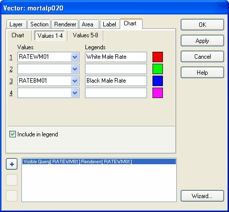
146 144

147 Tutorial The rendered result. The rendered result when the use of bar charts is selected. 145

148 Chart sizes The pie or bar chart sizes can also be rendered to reflect numeric values of a selected attribute field, or a formula based multiple attribute containing numeric values. This demonstration renders pie chart sizes based on the sum of the cardiovascular disease mortality rates for white and for black men. Therefore, the chart size shows the overall rate for white and black men together, while the colors within each pie chart show the relative mortality rates of black and white men. The Start size and End size values for the charts, which are defined in pixels, must also be specified under the Renderer tab. The result.

149 Tutorial Tutorial 7 - Label Rendering This tutorial demonstrates how to set up and customize the positioning, size, color, and other visual aspects of vector labels. Labels can be set up to show the information contained by any attribute. Note: In complicated map rendering situations, it is recommended to set up the label rendering first, before setting up the rendering of other aspects of the layer appearance Label Styles The Viewer can be used to set or alter the colors, size, transparency level, outline, text font, positions, etc. of labels. This demonstration uses a U.S. Department of Census TIGER vector line road/street map file. The procedure is the same for labeling vector points and polygon areas.

150 148 The information contained by any attribute can be presented in the labels. This example uses the labels to present street/road names, which are contained by the FENAME attribute. Note below that the FENAME attribute has been selected in the Field box under the Layer Properties' Label tab. Also pictured below, the label size and color are selected for all roads of the class A31. The road class information is contained in the CFCC attribute. Note that the labels for an entire layer can be tuned on/off, without changing the label rendering set-up, by checking/unchecking the Visible option.

151 Tutorial The result. 149

152 150 Now experiment with the label color. And with the label outline.

153 Tutorial 151 The result. If duplicate labels (more that one label for a single polygon in any map view) are not desired, the label duplication can be turned off by checking the Avoid duplicates option under the Label/Position tab.

154 Label Positions First of all, experiment with adjusting the position of the labels relative to the associated vector. Here the relative position is changed to position 1, from the original position 9.

155 Tutorial Rendered with the original label position

156 154 Rendered with label position 1. Now the label position is set to follow the vector line. Note that the Avoid overlap setting is activated as the default. This feature prevents labels of any layer, even when many map layers are open together, from ever overlapping.

157 Tutorial 155 The result. The Viewer program positions the label to follow the line, and tries to place the label in the best fitting position along the line, i.e., next to the straightest available segment of the line in any given view. Notice how the labels automatically reposition to the best fitting positions along the lines as the user pans or zooms in or out.

158 156 The label fonts can be customized in many ways. As shown below, a unique appearance is selected for the name labels of the streets with the classification A41. A unique font, color, and size is specified. A number of script types are supported, such as Greek, Cyrillic, Arabic, Hebrew, Central European, etc.

159 Tutorial 157

160 158 The result. California Ave. has been selected, resulting in the presentation of its attribute information in the attribute panel Polygon Label Positions As long as the flow option is checked in the window under the Layer/Properties' Label/Position tab, the Viewer attempts to always place the labels of polygons in "good fitting" locations, for any zoom level and view position. The Viewer does simply position the label at the polygon centriod position. The Viewer also does not render the polygon labels in the very best positions, because achieving the perfect placements would consume too much computational resources and unduly reduce the rendering speed with large data sets. The objective is to offer the best compromise between position quality and speed. As illustrated below, even with these very irregularly shaped polygons, the Viewer does a reasonably good job placing the pie charts and labels inside the proper polygon area. (The pie charts are positioned according to the positioning of the labels.) As pictured below, if a simple centriod approach were used, the chart and label for polygon 487 would probably fall inside polygon 473. Also, if the Avoid overlap option in checked in the Layer/Properties/Label/Position dialog box, the Viewer ensures that labels and charts never overlap, even if many layers are open together in a project.

161 Tutorial Tutorial 8 - Spatial Select This tutorial demonstrates some of the spatial selection techniques supported by the program, to provide an orientation to the possibilities Select versus Localize The Viewer offers two options to select a single object from vector map data - Select by Point and Localize. Select by Point can be used to select objects only from the vector map layer which is highlighted in the Legend panel. Localize can be used to select an object regardless of which layer it is in and regardless of the layer selected in the Legend panel. The Localize feature can be very useful when many layers of similar data are open together in the Viewer at the same time, making it difficult to figure out which layer contains which objects. Select an object. While in Select by Point mode, left mouse click on a vector contained by the layer which is highlighted in the Legend panel. (When in a select mode the mouse cursor will appear as a.) The selected vector object will become highlighted on the map and the attributes of the selected object will be presented in the Attributes panel.

162 160 Localize an object. While in Localize mode, left mouse click on a vector contained by any layer open in the Viewer. (As in Select by Point mode, the mouse cursor will appear as a.) The selected vector object will become highlighted on the map and the attributes of the selected object will be presented in the Attributes panel. The first image below shows the Viewer after the selection of a street from the line layer highlighted in the Legend panel using the Select by Point mode. The second image shows the Viewer after using the Localize mode to select a segment of forest from a polygon layer, which is contained by a layer other than the layer highlighted in the Legend panel. The Viewer has identified the object and automatically updated the Legend panel to highlight the layer which contains the "localized" object. Localize is the only selection tool that is layer independent.

163 Tutorial 161

164 Spatial Selection Modes In addition to the selection of a single vector object at a time, the Viewer offers a number of sophisticated options for the selection of multiple objects on a selected layer based on a spatial criteria. These operations are sometimes referred to as 'spatial queries'. Multi-Select by Point: While in Select by Point mode and with the Ctrl key depressed, select multiple polygon vectors (areas) together by pointing and clicking on each vector with the mouse pointer. The Viewer automatically calculates and presents the average, minimum, maximum, and sum of the values of each attribute field. As pictured below, the multi-select feature is used to select the eight highlighted polygon areas. The average, minimum, maximum, and sum of the area and perimeter attribute values for the group of selected polygon areas is visible in the attribute panel. Like with Select by Point tool, Localize can also be used with the Ctrl key to select multiple objects on the same layer. Select by Line: Use the Select by Line mode to draw a line to select all polygon areas which are intersected by the line. Double click to finish drawing the line. Note that the geometric Select Type used in this example is Intersect (interior-interior), which is one of the more commonly used select types. This select type performs the selection based on any intersection of some portion of the interior of the selection figure (the line) with some portion of the interior of the vector objects in the layer. As is visible in the image below, a number of other selection types are available to precisely define the relation between the selection figure and the vector objects in the map layer.

165 Tutorial 163 Select by Rectangle: Use the Select by Rectangle mode to select with the use of a drawn rectangle geometric figure. Draw the rectangle by mouse clicking on the map to place one corner of the rectangle and clicking a second time to place the opposite corner of the rectangle. (Alternatively, mouse click to place one corner and then drag the mouse cursor to the position of the opposite corner and release the mouse button.) As shown below, reflecting the Intersect (interior-interior) select type, all polygon areas with at least some portion of their interior in common with the interior of the selection rectangle are selected.

166 164 Select by Polygon: Use the Select by Polygon mode to perform a selection using a drawn polygon area. Draw the polygon by clicking with the cursor to place each corner of the polygon boundary. Double click when placing the final corner of the polygon boundary to automatically form the polygon area.

167 Tutorial 165 Select by Circle: Use the Select by Circle mode to perform a selection with the use of a drawn circle. Draw the circle by clicking on the map position for the circle center and dragging the curser to the placement of the circle perimeter. Depress the mouse button to finish. The following image shows the use of exactly the same selection circle as in the image above, but with the selection performed based on the Contains Select Type setting. The result is the selection of only the polygon areas which are fully inside (contained by) the circle.

168 166 The next image shows a selection by circle but using the Intersect (boundary-interior) Select Type. The result is that only polygon areas which are intersected by the perimeter (boundary) of the circle are selected. For the purpose of demonstration, the selection color (this setting is under the Tools/Options/Selection menu), has been changed from semitransparent red to semitransparent yellow.

169 Tutorial Copy & Copy Special to Clipboard Layer The Copy feature, which is accessed using the Copy toolbar icon (or the Edit/Copy menu command), is used to copy selected vector geometry to a Clipboard layer. The Clipboard layer is an 'in-memory' layer (without any normal file format) and contains only the vector geometry. Attributes are not copied to the Clipboard layer. Furthermore to the functionality demonstrated below, the Copy function also adds the selected vectors to the Windows clipboard using the EMF meta format. This provides for easy insertion into many other types of files, such as a Word document or to CorelDRAW. This example uses the results of the last spatial select operation from the prior section to demonstrate the Copy procedure.

170 168 As pictured below, the Copy feature (also available under the Edit/Copy menu) has been used to create a copy of the selected objects on a Clipboard layer. During the copying process, all the selected polygons were fused (via a union) into a single vector polygon. (In this image the visibility of the original polygon map layer is turned off in the Legend panel to more clearly show just the geometry that has been copied to the Clipboard layer.)

171 Tutorial 169 The Copy Special feature (also available under the Edit/Copy Special menu) provides for copying to the clipboard layer with more options to customize the result. By making the right source and copy type selections in the Copy Special combo box, map objects can be selectively added, subtracted, exchanged, or merged on the Clipboard layer. The Copy Special to Clipboard layer functionality is a powerful tool. Refer to the description of the Copy Special feature in the Help files for more detail on each of the Copy type options. The Selected shapes (individual) option, as selected in the image above, results in the selected polygon areas being individually copied to the clipboard layer, as multiple vector polygons.

172 170 Note that after a Clipboard layer has been created, the Select by Clipboard option under the Map/Select menu becomes active. This spatial select option allows the use of any geometry on the clipboard layer to perform a spatial selection on any selected map layer. The Clear Clipboard feature (also available under the Edit/Clear Clipboard menu) is used to remove all data from a clipboard layer. The Editor product (not supported in the Viewer) supports saving data from the clipboard layer to any supported vector format. A saved clipboard layer can later be reloaded to the Clipboard of either the Viewer or Editor program, using the Edit/Load Clipboard menu command Tutorial 9 - Attribute Query The search function may be used to query for vectors in a layer based on the information contained by an attribute or set of attributes. The query can reflect the following relationships: =, +, >, <, <>, <=, >=, and "like". Access the vector search functionality by clicking on the Show Search Panel toolbar icon (or using the Tools/Search menu command). The first example searches for any polygon in which the HSA_NAME attribute contains the text "Cook" (for Cook County, Illinois). Because the attribute field contains more text than just "Cook" (see the attribute panel below in the image below), the like search setting is used, which means that the search is not case sensitive. The "%" mark is added after the text "Cook" to substitute for the remaining information in the attribute field. The result is that the search is preformed against only the first few letters contained by the HSA_NAME attribute. Note that this search is limited to the visible extent area, but the search could also be performed on the entire map layer by just changing the setting. As shown below, the search operation properly found the Cook County HSA.

173 Tutorial 171 The attribute name field allows the selection of the attribute to be queried. The attribute name field contains a drop-down selection list with all attribute names contained by the vector layer. The attribute values field provides for the specification of the numeric or text values that are to be targeted by the search. The attribute values field contains a drop-down list of up to 256 actual values from the map layer contained by the selected attribute. A value from the drop-down list can be selected or enter a unique value can be entered to the field. If using unique value which is not contained in the drop-down list, press the Enter key to accept the value. Otherwise the program will auto fill this field with the value from the drop-down list which is closest to the entered value. The following is demonstration of the query of an attribute which contains numeric values. The search is for all polygon areas with RATEWM01 attribute values greater than 237. The HSA areas meeting this query definition are highlighted in the search result. As was explained in an earlier tutorial using this same file, the RATEWM01 attribute contains the heart disease mortality rate for white males. Therefore this query is for all HSA areas in which the annual mortality rate stemming from heart disease in the white male population is greater than 237 per 100,000. As can be seen from the statistical calculations presented in the Attributes panel, the average heart disease related mortality rate of the HSA areas selected by the query is per 100,000. The highest value from the selected group is and the lowest value is

174 172 The Viewer provide the SQL Query Builder tool to define more sophisticated queries. Check the Query box (pictured in the above screen image) to open the SQL Query Builder window. The SQL Query Builder provides for the definition of more complex queries, which can be based on multiple attributes. In this example the query is modified to search for all areas in which both of the following are true: - The mortality rate for white men is greater than 237 per 100,000 - The mortality rate for white women is greater than 135 per 100,000 The rendered result. (Obviously the mortality rate due to heart disease is significantly higher for men than for women.) As is visible in the Selected Attributes tab in the image below, the average rate for white men within the selected areas is per 100,000 and the average rate for white women is per 100,000.

175 Tutorial 173 This same SQL Query Builder window appears in other places of the Viewer/Editor program in which attribute queries may be performed, such as the Editor Layer Export and Layer Merge procedures Tutorial 10 - Measurement Tools The Viewer provides two ways to measure length/distance or the areas and perimeters of areas. One method calculates these measurements based on an already existing vector in an open layer. The second method calculates these measurments from a temporary line or polygon which is drawn on top of the other map layers. The map layer(s) must be in a projected coordinate system, with linear units (meters, feet, etc.), for the measurement to yield accurate results, becuase the measurement results are presented in the same units as the units used by the coordinate system. If, for example, the measurement were performed on a layer defined in longitude/latitude coordinates, such as the common WGS84 coordinate system, the measurement results will also be provided in coordinates, which is not meaningful. In the following image, the number of points, parts, length (which is the length of the perimeter in the case of a polygon), and area of the selected polygon are visible under the Shape tab in the Attribute panel. The data presented is calculated from the geometry of the vector object, and not from the information which may be contained by the attributes of the selected vector. The distance/area measurements are presented in 'map units', which are the same as the linear units of the projection.

176 174 The area/distance/perimeter measurement tool is opened by clicking on the Measure icon (or using Tools/Measure menu command). This tool allows the user to draw temporary line or polygon area that is to be measured.

177 Tutorial Tutorial 11- Export to Image file The Viewer supports advanced image file export functionality. The export to image procedure generates the export image from a specified extent (area) of the source map data, as the data is visibly presented in the Viewer map window. The source data can be composed multiple layers, which can be raster or vector, and reflects the rendering configurations set up in the layer properties. The export is generated only from the map viewer window, and does not include any of the panels (Attributes, Legend, MiniMap, etc.) which may be open. (The export to a PDF document file is explained in the Print, Print Preview, PDF tutorial.) This demonstration uses a vector world map with the color of each country rendered at random. As illustrated below, the visible extent is zoomed in to the region of the Arabian Peninsula. This visible map extent will be exported to an image file. Begin the export procedure by clicking on the Export to image toolbar icon (or using the File/Export to image menu command). The Viewer will advance to the Export to image... window, which allows the user to enter a file name for the image to be created by the export procedure and select the format (file type) of the export image. The PNG file type is selected for this exercise. (The PNG format is a good compression format choice for source data with a limited number of colors, like with this situation.) Click on the Save button to proceed to the Export to window.

178 176 The Export to window provides for the selection of the extent of the source data to be exported from and the file type, resolution, and compression level of the export image that is to be generated. (With 8-bit and Best Quality selections, the estimated size of the data to be exported is MB.) Export Extent:

179 Tutorial 177 The extent of the source data that is generated to the export image can be defined in two ways: - Full: The full extent of all open map layers. - Visible: The extent that is presently visible in the map viewer window. The Editor product also offers a more precise extent selection method, called User defined, which is based on coordinate values, i.e., an upper and lower y coordinate value and a right and left x coordinate value. Export Resolution: To make the selection of the export resolution as simple as possible, buttons are provided for the selection of the three most useful export quality levels: Best Quality, For Document, and For Web. Best Quality - If generating the export image from a raster image layer, or a source data set including a raster image layer, this setting generates the export image at the same resolution level (pixel density) as the source image. If the source data contains image layers of different resolutions, the Best Quality setting generates the export image at the resolution level equal to the source image layer with the highest resolution. (This situation will result in some up resampling of the portions of the export image generated from raster layers of lower resolution levels.) If the export is generated only from source layers containing vector data (like in this demonstration), the Best Quality setting generates the export image with 4,000 pixels in the width and with the number of pixels in the height proportionate to the height-width ratio of the source extent. For Document - This setting generates the export image with a resolution level that is of a reasonable quality (versus the file size) for use as a typical physical document, which is a width of 14 cm and a DPI (dots per inch) of 300. The number of pixels in the height will be proportionate to the height-width ratio of the source extent. For Web - This setting generates the export image with a resolution level which is the maximum that is typically web published pixels in the width and the height proportionate to the heightwidth ratio of the source extent.

180 178 (With the For Document resolution setting, estimated size of the data to be exported is only 2.7 MB.) In addition to the three, one-button export resolution settings, the export resolution can be custom defined based on either i) the number of pixels in the height and width of the image or ii) the image height and width in measurement units (inches, centimeters, or millimeters) in combination with the DPI. The second option can be useful if the export image file is to be printed, such as by a professional printing shop. This window provides an advanced estimate of the size of the export image file to be created approximately 2.7 MB in this example - before any compression is performed in the event that the export is generated to an image compression file type, e.g., JPEG, PNG, or TIFF-LZW. If the source data includes a raster image layer and the Best Quality setting is selected, the estimated size will reflect the resolution of the source raster image, the selected export extent, and bit level of the export image. (Note that the information about the height and width in pixels of any image opened as a layer in the Viewer can be found under the menu Layer/Properties/Layer/Info.) If the resolution (pixel density) of the export image is specified by the user, such as with the use of the For Document or For Web options, the resolution of any raster image layers in the source data has no bearing on the size of the export image. Depending on the level of any JPEG, PNG, or TIFF-LZW compression applied during the export process, the actual export image file size can be significantly less than the estimated size before compression. In this example, the PNG compression reduced the exported PNG image file to only 66 KB. Below the exported PNG image is opened in another commercial image viewing software product.

181 Tutorial 179 Image Registration files: During the PNG export process, the Viewer also generates a *.PGW file (a World File) and a *.TAB file (TAB registration file). These files contain information about the coordinate system of the exported image to allow the exported image to be correctly opened in other GIS software products which understand geographic coordinate systems. For example, the image below shows the exported PNG image opened in the Viewer as a separate layer over the original vector map layer. The PNG image is automatically positioned correctly relative to the vector map layer. Without a *.PGW or *.TAB file (some GIS software programs understand the *.PGW format and others the *.TAB format; TatukGIS products understand both file types), the program would not know where to position the PNG image. The Viewer generates an associated World File and TAB registration file with any exported image, but the file endings are different for each format, e.g., TIFF, JPEG, BMP, etc. To work properly, the World File and/or TAB registration file must be kept in the same file folder as the image file. When the export is to the TIFF format, the Viewer also generates the TIFF as a GeoTIFF, thereby embedding the coordinate information within the TIFF file itself. In the image below the exported image has been opened as a layer on top of the original vector world map layer. The vector world map has been rendered grey color to highlight the proper placement of the PNG image file.

182 180 Size considerations when exporting to JPEG and PNG files: The export of more than 25 MB, before compression, to JPEG or PNG files is generally not recommended. The export of larger sizes to JPEG or PNG can work OK in some situations, but in other situations the resulting image may not open or work properly in some software products. Certainly the export of over 100 Mb to the JPEG or PNG formats is risky. If size is an issue, consider exporting instead to the TIFF or BMP formats, which have no inherent size limitations. The Viewer also exports to TIFF with LZW compression, which has no inherent size limitations. Alternatively, consider using the PixelStore image format, which is designed by TatukGIS specifically to efficiently handle huge images Tutorial 12 - Export Image Mosaics Multiple georeferenced image files can be opened as separate layers in the Viewer and viewed together and saved together to a single image file. The starting images must be in the same geographic coordinate system so that the Viewer knows how to position the images relative to each other and well rectified so that they mosaic together nicely. This Tutorial uses two standard U.S. Geological Survey DOQQ aerial TIFF format images. Each image is paired with an associated World file (*.TFW) which contains the coordinate system information for the image.

183 Tutorial 181 Although this example shows the mosaicing of only two images, there is no limit on the number of images that can be opened together in the Viewer or exported to a single image mosaic. Below a single TIFF image is opened in the Viewer. Now second TIFF image, of territory that is adjacent to the territory of the first image, is opened as a second layer in the Viewer.

184 182 As explained in the prior tutorial, click on the Export to image toolbar icon (or use the File/Export to image menu command) to select the file path for the export file and to open the Export to... window. The parameters for this image export are defined as pictured below. The export is to be generated to a 24-bit TIFF with LZW compression. The Best Quality master setting has been selected, which will create the export image at the same resolution level as the source images. (Refer to the Layer/Properties/Layer/Info dialog box to check the resolution information for the source images.) (As shown in the window below, the total uncompressed file size being exported is only approximately 2 Mb, because the resolution of the images used for these screen shots was previously reduced from the original DOQQ TIFF aerial images provided by the U.S. Geological Survey. The original images were each well over 100 Mb.)

185 Tutorial 183 The exported result - a TIFF mosaic, with LZW compression. Note in the Legend panel that now only the single TIFF image layer is open in the Viewer. (The text "Exported with the TatukGIS Viewer: in yellow color is added in the lower left corner of the exported image.)

186 Tutorial 13 - Print, Print Preview, PDF Any map view can be printed directly from a local printer or printed to a map quality Adobe Acrobat PDF (a vector format) file that can be saved. This tutorial demonstrates these procedures using the same map data and map view as used in the earlier Export to Image File tutorial. In addition to the PDF file generation demonstrated here, the Copy feature (access with the Edit/Copy menu command) can be used to copy the visible extent to the Windows clipboard as an EMF file, for inclusion to a Word document, CorelDRAW, etc. The printing is performed to the same scale as the map appears in the map viewer window just before starting the printing procedure. Refer to the Scale Setting instructions under the Viewer Main Menu controls for more information about the scale setting. Click on the Print Preview toolbar icon (or use the File/Print Preview menu command) to start the print procedure. The print preview step can be skipped by instead using the Print toolbar icon (or the menu File/Print menu command). The Print Preview dialog box allows the user to enter a title and subtitle that may be printed in the lower left corner of the map, and to determine whether to include the date, scale, Legend, and MiniMap in the printed output. The print functionality always prints the visible extent, or an area just large enough to capture at least the visible extent after any height/width re-sizing. Click on the Print button. Printing can include the Legend and MiniMap panels, but cannot include the Attributes information panel.

187 Tutorial 185 The next dialog box allows the user to customize the printer set-up options, if required. Use the Print to PDF toolbar icon (or the File/Print to PDF menu command) to advance to a

188 186 print preview dialog box that is similar to the one shown above but with the Print to PDF button, as pictured below. Click on the Print to PDF button to generate a PDF file from the selected extent. Below the exported PDF file has been opened in Adobe Acrobat Reader.

189 Tutorial Tutorial 14 - URL Referencing Vector objects in any vector map layer can be referenced to other files (images, documents, etc) or web pages using the URL hot-linking feature. This allows a project to be set up a so that if the user double-clicks on a vector point (such as represented by a symbol), polygon area, line segment, etc. while in localize or select by point mode, the Viewer automatically links to the associated file. The linkage can be to document or image file, a web site address, or even to automatically launch a pre-addressed via Microsoft Outlook. The following images show the linkage of one symbol representing the location of a cafe with a JPG image of the cafe stored on the C drive of the computer at the file path location: file://c:\photos\blue Poodle Cafe.jpg. Note that this file link has been recorded in the photo attribute field. (Of course, the URL information cannot be added to the attribute field using only the Viewer itself, because the Viewer does not support attribute editing. The URL information can be set up using the TatukGIS Editor or any other software with GIS editing capabilities. The Viewer can then be used to distribute the project with the URL referencing to final users.)

190 188 When the user double-clicks on the symbol, the following image of the cafe is automatically launched. The URL linkage mechanism refers to the first URL link address contained by any attribute field for the vector object.

191 Tutorial 189 To link to a web page, enter the information to the attribute field like: For example, to link a map object to the TatukGIS home page, the URL would be entered as: To launch a pre-addressed , enter the information to the attribute field as: mailto:... For example, if the is to be sent to TatukGIS, use: mailto:sales@tatukgis.com. An option to turn off the URL hot linking functionality is available under the Tools/Map hotlinks menu. Uncheck the (URL) auto check box to turn hot linking off.

192 Editor Tutorial 1 - Main Menu Controls This image shows the most important menu controls which are unique to the Editor, i.e., not already covered in the Viewer tutorials. Because the TatukGIS Editor supports all the functionality of the TatukGIS free Viewer, also refer to the Viewer Menu Control descriptions. A U.S. Department of Census TIGER street map data layer is open in the Viewer. The streets have been rendered by color and width based on the CFCC (street type) attribute. This image shows the Editor with the Show Data Panel option activated to present the attribute information for the street vectors located in the selected area (the circle) in a grid table, for viewing or editing from the table or for export to a spreadsheet or database product.

193 Tutorial 191 The Options... combo box of the Editor program includes one additional tab - the Editor tab which is not part of the Viewer. This the window under this tab, which can be accessed using the Options toolbar icon (or the Tools/Options menu command), allows three program settings which are specific to editing of vector geometry to be turned on/off. - The Show Tracking Points feature shows the vertices (points) forming all vectors on the layer that is being edited. - The Show Points Numbers feature shows the numbers of the vertices (points) of any vector object that is selected in edit mode. - The Wire Mode feature shows the effect of the addition of a new vertex (point) on an existing polygon before the new vertex is actually created. - The Auto apply data table changes feature records editing changes performed in the table in the Data panel even if the user does not click on the OK button at the top of the Data panel when finished. If checked, the OK button at the top of the Data panel will not appear.

194 Tutorial 2 - Digitize New Map Geometry This tutorial shows how to create new vector data layers and the ways to add vector data to layers. It demonstrates the creation of new polyline and polygon vector map layers on which new vector geometry will be manually drawn using the program's editing features, with the use of a rectified and georeferenced aerial image as a background layer. This process of creating new map data is sometimes referred to as "digitizing" or "vectorizing". Although this tutorial shows the creation of polyline and polygon data, the procedure for creating point and multipoint layers is digitizing new point data to the layers, is essentially the same Create New Vector Layer The create new layer procedure creates a new and empty vector file which is automatically loaded as a layer in the Editor. The file type (format) of the new layer is selected at the time of its creation. The new layer can then be populated with vector geometry in two ways: 1) use the Layer/Import menu to import an already existing file into the new layer or 2) 'digitize' new vector map data from scratch using the Edit mode drawing tools. Either way, the data added to the new layer will be in the format which is specified when the layer is first created. If an existing vector map file of a different format is imported into the layer, the data will be automatically converted to the format of the layer during the import process. The following demonstrates the digitizing of vector data to the new layer, using an orthorectified (high accuracy) aerial photo as a reference layer. The screen image below shows a black and white, MrSID format, aerial image opened in the Editor. The MrSID image covers an entire county in the United States, but the view is zoomed in on the area of a local neighborhood subdivision.

195 Tutorial 193 Use the Layer/New menu command to open the Create New Layer... window. Select the file path from the Save in field and the file name in the File name field. Select the file type (format) for the new vector layer by selecting from the supported vector file types listed in the drop down list in the Save as type field.

196 194 The Editor can create new layers to a choice of the following file formats. The format option at the bottom of the list, TatukGIS SQL Layer(*.ttkls), is for exporting the layer to a SQL geodatabase file. The default database configuration exports the vector layer to a Microsoft Access database file with a choice between two formats: i) SQL Native, which is TatukGIS binary SQL method, or ii) SQL OpenGIS (WKB), which is with OpenGIS Simple Features for SQL Implementation. When creating SQL based geodatabase layer, select a file name without any spaces or unusual characters. This is to ensure that the file name is compatible with the various SQL database products. The layer can be exported to i) SQL database products other than MS Access (such as MYSQL, Oracle, DB2, Interbase, MSSQL, etc.) or ii) the Geomedia SQL Server Warehouse format, only

197 Tutorial 195 by manually customizing the SQL database connector (*.ttkls) files. The creation of a SQL geodatabase layer in one of these SQL server database products, or in the Geomedia SQL Server Warehouse format, would typically indicate a multi-user environment and require an administrator to create and manage the database connections/configuration. (For some more details on setting up the SQL database connector (*.ttkls) files, refer one of the FAQ items relating to this topic.) When the Save button in the Create New Layer... window is selected, the Create New Layer dialog box automatically appears. This dialog box allows the user to specify 1) the type of vector geometry - Point, Multipoint, Line, or Polygon - the layer is to contain and the 2) extent of the layer. The default extent, as shown below, reflects the total extent all the layers currently open in the Editor, and is defined by the x axis coordinate of the let and right boundaries by the y axis coordinate of the top and bottom boundaries. Generally these x and y extent values will reflect the coordinate system of the layer(s) currently open in the Viewer, assuming that the layer(s) are in a geographic coordinate system. Since, in this example, only the single image layer is open in the Viewer, the default extent settings for the new vector layer reflect the extent of the georeferenced MrSID image. As seen in the Legend panel below, the newly created (and empty) polyline file has now been opened as a layer in Editor.

198 196 At any time layers can be added or removed from the program by using the Add layer toolbar icon (or the Layer/Add menu command) or the Remove layer toolbar icon (or the Layer/Remove menu command) Create Vector Polyline Data Start drawing vector data to the newly created layer by i) highlighting the new layer in the Legend panel and ii) clicking on the edit modes toolbar icon. (Alternatively use the Shape/Edit mode menu). When in the default Edit mode, this toolbar icon appears as a. Then select the desired editing mode from the drop down list. Notice that not all edit modes are activate for polyline layers. The edit modes which are activate (appropriate) for polyline layers are presented in the drop down list in bold black, whereas the drawing modes which are inactive (inappropriate) for polyline layers are presented in light gray color. These inactive edit modes will become active when working on layers containing other types of vector geometry, e.g., points, multi-points, or polygons.

199 Tutorial 197 Because this demonstration involves the creation of line vectors to represent irregular street patterns, the Line edit mode option is appropriate. The edit mode icon will convert from the default Edit mode to Line mode. The Line icon will remain in place until a different edit mode is selected or the user returns to Select edit mode. The edit mode icon always appears as the icon corresponding to the currently selected edit mode. The all the available edit modes are presented in the drop down list next to the edit mode icon in the toolbar.

200 198 Then zoom in to a comfortable level at the proper place on the image and start placing the vertices (points) to form the lines. This is done by positioning the curser (which now appears as a ) and clicking with the left mouse button. Use the zoom or drag mode tools to reposition the visible map area when necessary. The user can drag without leaving the edit mode by temporarily depressing the Shift key and dragging the image with the mouse cursor. The user can zoom in/out without leaving the edit mode by temporarily depressing the Alt key and dragging the cursor in the upward direction on the map (to zoom out) or the downward direction on the map (to zoom in). The mouse wheel can also be used to zoom in/out without leaving the edit mode. Another option is to activate the Auto Center feature under the Tools/Options/Map menu. When activated, the Auto Center feature automatically repositions the map area in the viewer window to center on the place of the last mouse click. This eliminates the need to reposition the map view because the editing process has neared the edge of the view extent. To complete one line and begin another, simply click on the Line icon in the toolbar and start drawing the next line. This allows for the rapid completion of one vector line and the starting of the next one. The following screen view shows portions of two streets that have been digitized as vector polylines. The green polyline with the numbered vertices appears so because it has been selected using Select edit mode. Notice that information (length, number of vertices, number of parts) about the selected polyline is presented under the Shape tab in the Attribute panel.

201 Tutorial 199 If a vertex is misplaced or some other mistake is performed during the process of editing a vector, the mistake can be quickly corrected by clicking on the Undo toolbar icon. Undo cancels the action performed by the last mouse click. Click on Undo a second time to also cancel the action performed by mouse click before the last one. Click on Undo a third time to also cancel the mouse click before that one, etc. If a vertex is inaccurately placed, it can also be repositioned by depressing the right mouse button and dragging the selected vertex to the accurate position, then releasing the mouse button. Any vertex of a vector selected in Select edit mode can be deleted by left clicking while holding the mouse curser over that vertex. All geometric changes made to any vector since the last time that data was saved can be cancelled (reversed) in one quick step using the Revert Shape feature. First select the vector to be reverted while Edit mode, then perform the reversion on the selected vector by clicking on the Revert Shape toolbar icon (or using the Shape/Revert Shape menu command). The Revert Shape feature can be used on any vector that has been edited since the last time the data was saved. The function is not limited to the last edited vector. When creating vertices to form a polyline, if any vertex placement is at greater than a 90 degree angle from direction of the last-created line segment, the Editor program will assume that the intent is to insert the new vertex between two already existing vertices, as pictured below. Starting polyline. The program inserts the new vertex between two already existing vertices.

202 200 If the intent is to connect the new vertex to the last-placed vertex, this can be achieved by depressing the Ctrl key while mousing clicking to generate the new vertex. The result is pictured below. As the polylines are created, the snapping feature can be used to automatically close the intersections of the vector polylines. The snapping feature automatically positions the placement of the new vertex at exactly the same place an any vertex of another vector located very nearby. Without snapping it would be very difficult to exactly join intersecting polylines at intersection points - there would always be a small gap or small overlap which would be visible at a very close zoom level. The snapping is performed only to nearby line vertices, and not to any segment of a line between the vertices. (When the first vertex of a new polygon is drawn, all the vertices in the snap-to layer will become highlighted as yellow colored points.) Snapping may be performed to the vertices of any vector layer that is open in the Editor. The "snap-to" layer is selected from the drop down list located on the toolbar just to the right of the edit mode icon. The following images shows that even at very, very close zoom levels, the closure at the intersection point is perfect. Line intersection at a close zoom level.

203 Tutorial 201 Line intersection viewed at an even closer zoom level. The user can temporarily override the snapping feature by depressing the Ctrl key when mouse clicking to place a vertex. This is important for situations in which new vertices must be placed at unique locations which are extremely close to, but not the same as, already existing vertices. In addition to the creation of the polyline map geometry, attributes such as street names, street types, etc. can be assigned to each individual polyline. The UID record names (the left column in the Attributes panel when the Attributes tab is selected) are the same for all polylines (true for any vector type) in a layer. The value fields (the right column in the Attributes panel) may contain unique information for each individual vector. To add an attribute to contain a value field for each vector in a layer, first select (highlight) the appropriate layer in the Legend panel and select a vector in the layer to make the attribute information appear in the Attributes panel. information. Then right click in the UID column in the Attributes panel. (The Show Data Panel option must be turned off when doing this.) Three options will appear as follows: Select the Add field option to open the Add field window and enter the required information to create new attribute for the layer. The unique value field for each vector object (such as the

204 202 name) must be entered in the right column in the Attribute panel, after selecting the vector in the layer. For more information on editing attributes, refer to the Editor "Editing Existing Map Data Attribute Editing and Restructure" tutorial. The next image is after the streets in the neighborhood have all been digitized. As is visible in the Attributes tab within the Selected panel, attribute information has been assigned to the selected line (the line with the green numbered vertices). After entering attribute information for a vector, click on the OK button in the Attributes panel to accept the entered information. Then the attribute information will be saved with the vector geometry the next time that the vector layer is saved. Notice in the image below that the text "Morgan Co MrSID.ttkgp" at the top of the application window has replaced the text, "noname.ttkgp", which earlier appeared in this place. This means that the data set open in the Editor has been saved as a TatukGIS (*.ttkgp) project file with the file name "Morgan Co MrSID.ttkgp". The default "noname.ttkgp" only appears in this place until the data set open in the program has been saved as a TatukGIS project file. Any data set open in the Viewer/Editor can be saved as a TatukGIS project file using the File/Save Project As menu. Use the Save All toolbar icon (or the File/Save All menu) to save all changes to the vector layers. Use the File/Save menu to save changes only to the layer that is selected in the Legend panel.

205 Tutorial Create Vector Polygon Data This section demonstrates the digitizing of vector polygon areas. Some elements of the editing procedure are explained in more detail in the prior section demonstrating line digitizing. It is best to review the prior section first. Polygon vectors to will be drawn to represent the crop fields in the area of farmland captured in an a MrSID format aerial image. As is visible below, the MrSID image titled "cooper" is opened in the Editor. First create a new vector layer, as was demonstrated in an earlier section of this tutorial, but this time select that the layer be for polygon data. As is visible in the Legend panel of the image below, the new (and empty) polygon vector layer named "Vector layer polygons" has been loaded to the Editor. The vector layer is positioned on top of the aerial image layer so that the polygons to be created will be visible on top of the aerial image.

206 204 With the vector layer highlighted in the Legend panel, select the Polygon down edit mode list in the toolbar. mode from the drop Zoom in to a comfortable level in the appropriate place and begin placing the vertices to form the polygons by positioning the curser (which now appears as a ) and right clicking with the mouse. To complete one polygon and begin another, just click again on the Polygon icon and

207 Tutorial 205 start forming the next polygon. Note that the default Edit icon has been replaced in the toolbar by the Polygon icon. The Polygon icon will remain in that place until the user changes the edit mode. The user can drag (pan) the image without leaving the edit mode by temporarily depressing the Shift key. The user can zoom in/out without leaving the edit mode by temporarily depressing the Alt key. The following screen shot shows the partial vectorization of one of the farm fields on the image. The next image shows a completed polygon, formed by six vertices numbered 0-5. Notice in the Attribute panel that the attribute editing functionality has been used to create a layer attribute to assign unique names (identifiers) for each polygon. The polygon area selected in image below has been assigned the name "J".

208 206 Polygons have been created to represent eleven fields of this farm, named "A" though "K". Farm field "D" is selected in the image below. The layer properties have been used to render the polygon interiors as fully transparent and the polygon perimeters as thick blue lines. The automatic snapping feature during the editing process allows contiguous polygons to be

209 Tutorial 207 quickly created without error, by simply using the vertices from the adjacent polygons to position the vertices of the adjacent polygon. (The snapping mode can be temporarily deactivated by depressing the Ctrl key when mouse clicking.) The placement of the vertices can be snapped to the positions of vertices contained any open layer by selecting the snap-to layer from the drop down list in the toolbar located just to the right of the Edit mode icon. Information other than just the vector attributes can be viewed in the Selected panel. In the following view the Points tab within the Selected panel is opened while a polygon is selected in Edit mode. The x,y coordinates of each of the six vertices forming the selected polygon can be viewed and edited from the list in the panel, thereby altering the geometry of the selected polygon. In this way a polygon can also be created from scratch by simply entering a series of x,y coordinates.

210 208 Below the x coordinate of vertex number 1 has been increased from to , with immediate effect on the polygon geometry. New points can be added to the selected polygon by right clicking on the table under the Points tab. The entire coordinate table can be copied and pasted to a document or other file or exported/imported to/from another source. (Refer to the Joining Attributes tutorial.) As shown in the next image, the Shape tab within the Selected panel provides other information about the geometry of the selected polygon, e.g., the total number of points (vertices) that form the polygon, the number of parts, the length of the polygon perimeter, and the polygon area. The perimeter length and area information is provided in map units, which reflect the coordinate system of the layer or project opened in the program. (In this case, the coordinate system is the coordinate system of the MrSID aerial image which was initially opened in the Editor.) Note that the number of points (vertices) of a polygon as shown under this tab is always one more than the number of vertices that can be edited. This is because the final vertex is exactly in the same position as the number 0 vertex. This ensures proper closure of the polygon.

211 Tutorial 209 Use the File/Save all menu (or the Save all icon) to save the newly created vector data or changes. The File/Save menu can also be used if the intent is to save only the selected layer Delete Vectors To delete a vector, using the Edit toolbar icon (or the Shape/Edit mode/edit menu command), first select the vector by clicking on it. In the image below, the polygon representing Field A is selected while in Select edit mode.

212 210 Then click on the Delete shape toolbar icon (or use the Shape/Delete Shape menu command) to delete the selected vector (shape). (The deleted vector will be permanently deleted only when the data is next saved.) In the image below, the Field A polygon has been deleted from the polygon layer. As a data protection feature, vectors can only be deleted when in Edit mode. If the a vector or vectors are selected in any other way, such as using the Select by Point tool or via an attribute query, deletion of the selected vector or vectors is not possible. Use the File/Save All menu command to permanently delete the deleted vectors from the saved file Custom Edit Modes The Editor offers a number of useful tools to easily draw special features that might have to be created repeatedly when digitizing vector map data. The following special drawing tools can be found under the Shape/Edit Mode menu or by clicking on drop down list next to the default Edit icon. Edit modes for polyline layers: Edit modes for polygon layers:

213 Tutorial 211 As with the creation of standard points, lines, and polygons, some figures can be finished and the next figure begun by clicking on the relevant edit mode icon in the toolbar. For the figures composed by a finite number of vertices, the next figure can be started even without returning to the edit mode icon in the toolbar. Some other figure types can be completed (finished) by double clicking. The following vector outline figures can be drawn on a polyline layer: Rectangle outline (use the edit tool) Mouse click where two opposite corners are to be placed (or left mouse click, drag, and release). Rectangle automatically competes after placement of the second corner (or if done by dragging, upon release of the mouse button). Rotated rectangle outline (use the edit tool)

214 212 Place the locations of three corners with mouse clicks. Rectangle automatically competes after the placement of the third corner. Line with all right angles (use the edit tool) Series of left mouse clicks. Double click to close the figure (to make a closed polygon outline), if desired. Circle outline (2 techniques for circle drawing are provided)

215 Tutorial 213 Technique 1 (Circle using the edit tool): Left mouse click, drag and release. Circle completes upon release of mouse button. Technique 2 (Circle 3 point base using the edit tool): Left mouse click on three points to be placed on the circle perimeter. Circle completes after placement of the third point. Free line (use the edit tool) Right mouse click, drag, and release. Reposition the curser and start dragging again to continue the same line from a new place, with a straight line segment connecting the free line segments. Double click can be used to complete the formation of the line. The following polygon vector figures (areas) can be drawn on a polygon layer: Rectangle polygon area (use the edit tool)

216 214 Mouse click to place two opposite corners of the rectangle (or mouse click, drag, and release). Rectangle automatically competes after placement of the second corner (or if done by dragging, upon release of the mouse button). Rotated rectangle polygon area (use the edit tool) Place the locations of three corners with mouse clicks. Rectangle automatically competes after the placement of the third corner. Polygon 90 degree, for creating polygons with multiple 90 degree angles. All angles are 90 deg. except for the two angles formed by the closure side of the polygon. (Use the edit tool.) Series of clicks. Double click to close. Circle polygon (2 techniques for circle drawing are provided)

217 Tutorial 215 Technique 1 (Circle using the edit tool): Left mouse click, drag and release. Circle completes upon release of mouse button. Technique 2 (Circle 3 point base using the edit tool): Lift mouse click on three points to be placed on the circle perimeter. Circle completes after placement of the third point Line/Polygon Smoothing The Smooth Shape function is used to convert a normal polyline or polygon perimeter into a smoothed line or polygon perimeter. This feature can be very useful in some occasions, such as to present the projected routes of a ships or airplanes. The following image shows a typical polyline created in the Editor.

218 216 While in editing mode, select a line or polygon vector and then click on the Smooth shape toolbar icon (or using the Shape/Smooth shape menu). As shown in the next image, this results in a preview presentation of how the line will appear after smoothing is applied and opens the BSpline tab within the Attribute panel. In this example, the default smooth factor setting of 10 will generate a smoothed vector line formed with 90 points (vertices). The smooth factor may be customized by increasing or decreasing the number of vertices used to form the smoothed line, as desired. Click on the Apply button to replace the previous line with the new smoothed line, as presented in the image below. In the next image the soothed line has been selected using the Edit tool to illustrate how the

219 Tutorial 217 smoothed line is still a normal vector polyline, but one formed by many well placed vertices Create Vectors Using COGO COGO is a system of using bearings and distances to define a course line or other vector geometry. The Editor COGO functionality can be used to define vectors in terms of bearing and distances from vertex to vertex, as opposed to using x, y coordinates to define the location of each vertex. The creation (editing) of vector geometry - polylines and polygons - can be performed by entering a series of bearing and distance information. This demonstration uses an actual courthouse land parcel deed record from the state of Iowa in the United States to plot the parcel over a georeferenced topological map and a orthorectified GeoTIFF format aerial image. Both of these raster layers are in the NAD83 Iowa State Planes, North Zone, US Foot geographic coordinate system. The survey description for Parcel B provided in following Plat of Survey is used to draw the boundaries of Parcel B to a new vector polyline layer. (The parcel could also have been drawn as a vector polygon.) The Plat of Survey information is as follows: PLAT OF SURVEY 1 PARCEL B IN PART OF THE N1/2 OF NW1/4 OF SECTION 23, TOWNSHIP 85 NORTH, RANGE 4 EAST OF THE 5TH PRINCIPAL MERIDIAN, JACKSON COUNTY, IOWA SURVEY DESCRIPTION: PARCEL B THAT PART OF THE NORTH HALF OF THE NORTHWEST QUARTER OF SECTION 23, TOWNSHIP 85 NORTH, RANGE 4 EAST OF THE 5TH PRINCIPAL MERIDIAN, JACKSON COUNTRY IOWA, DESCRIBED AS FOLLOWS: - COMMENCING AT THE NORTHWEST CORNER OF SAID SECTION 23: - THENCE NORTH 87 DEGREES 22 MINUTES 04 SECONDS EAST (ASSUMED BEARING) FEET ALONG THE NORTH LINE OF THE NORTHWEST QUARTER OF SAID SECTION 23 TO THE POINT OF BEGINNING; - THENCE CONTINUING NORTH 87 DEGREES 22 MINUTES 04 SECTIONS EAST FEET ALONG SAID NORTH LINE; - THENCE SOUTH 02 DEGREES 37 MINUTES 56 SECONDS EAST FEET; TO THE SOUTHERLY RIGHT-OF-WAY LINE OF COUNTY ROAD E17 (150TH STREET); - THENCE SOUTH 21 DEGREES 36 MINUTES 39 SECONDS EAST FEET;

220 218 - THENCE SOUITH 30 DEGREES 39 MINUTES 54 SECONDS EAST FEET TO THE NORTHERNMOST CORNER OF THE PARCEL OF RECORD DESCRIBED IN THE WARRANTY DEED DATED SEPTEMBER 17, 1971 AND FILED SEPTEMBER 21, 1971 AT BOOK 113, PAGE 44 AT THE JACKSON COUNTY RECORDER'S OFFICE; - THENCE SOUTH 58 DEGREES 32 MINUTES 06 SECTIONS WEST FEET ALONG THE NORTHWESTERLY LINE OF THE SAID PARCEL TO THE WESTERNMOST CORNER OF SAID PARCEL; - THENCE NORTH 34 DEGREES 45 MINUTES 57 SECONDS WEST FEET; - THENCE NORTH 10 DEGREES 34 MINUTES 17 SECONDS EAST FEET TOO THE SOUTHERLY RIGHT-OFWAY LINE OF COUNTY ROAD E17; - THENCE NORTH 02 DEGREES 37 MINUTES 56 SECONDS WEST FEET TO THE POINT OF BEGINNING. SAID PARCLE B CONTAINS 5.40 ACRES MORE OR LESS, INCLUDING 0.38 ACRES OF COUNTY ROAD EASEMENT ACROSS THE NORTHERLY PORTION THEREOF. The two screen views below show the topographical map layer (USGSSpingbrook) and the aerial image layer (Spingbrook) open in the Editor. In the first view the topographical map is positioned as the top layer and in the second image the aerial image layer is positioned on top.

221 Tutorial 219 The trickiest step in this exercise is identifying the starting reference point, "THE NORTHWEST CORNER OF SAID SECTION 23", as accurately as possible on either the topographical map or the aerial image. The boarders of Section 23 are marked on the topographical map, but the topographical map is less accurate than the orthophotomap image. It would be very helpful if the actual coordinates for the northwest corner of Section 23 (the reference point) were known. Unfortunately this information is not provided in the survey description. Create a vector polyline layer as shown in Editor Tutorial 1. Begin by manually placing the reference point on the raster map with the Points tab selected in the Attribute panel, and then switch to the COGO tab to enter the first bearing and distance call from the survey description. This first bearing/distance call has been entered in the screen image below. Notice that the bearing definition provided the survey description (North 87 degrees 22 Minutes 04 Seconds East) had to be manually converted to degrees in the degree system. (A later update of the Editor will allow the input of such deed call bearings in the original format.) Also note that the first vertex, No 0, is always represented by x,y coordinates in the table under the COGO tab, even though this is technically incorrect because the names at the top of these columns are Bearing and Distance. (This is because of the difficulty of showing different column names for only the first vertex.) All vertices other than No 0 in the table under the COGO tab are presented in terms of bearing and distance.

222 220 The result is as appears below. To make this first line segment clearly visible, the layer properties of the new Parcel B polyline layer have been set to render the lines bright blue and with a 2.0 pixel width. Continue entering the bearing/distance calls into the table under the COGO tab to continue drawing the Parcel B boundaries. The Attributes panel/cogo tab can be moved from the Editor to another place on the desktop and resized during the data entry process, if the user finds this more convenient. The table under the COGO tab appears as follows after all the bearing/distance calls have been entered. At this time, note that the absolute option has been selected for the Bearing data and the relational option has been selected for the Distance data. There are two options - absolute and relational - for entering both the Bearing and Distance data. The meanings of these settings are as follows: Bearing - absolute: The angle is measured starting from absolute North (0 degrees) in a 0-360

223 Tutorial 221 degree manor. Bearing - relational: The angle is measured starting from the direction of the last line segment, in a degree manor. (The direction of the last line segment is considered to be 0 degrees.) Distance - absolute: The distance of each vertex is measured from the first/beginning vertex of the vector, not from the previously numbered or nearest vertex. Distance - relational: The distance is measured from the previously numbered vertex. The completed parcel boundary line generated from the above bearing/distance calls appears below, while the line is still selected in edit mode. The closure of the final vertex (point No 9) with the "Point of Beginning" (vertex No 1) is not perfect, but the closure error is very, very small approximately 0.3 feet. (The Ctrl key was depressed when the OK button was clicked following the entry of the final call, to prevent the automatic snapping of the final vertex No 9 to the "Point of Beginning" vertex No 1.) This small error could be explained by an inaccuracy in the conversion of the bearings to the scale or it could reflect a small mistake or rounding error in the survey description itself. A non closure by a few inches is insignificant.

224 222 The appearance of the land parcel boundary over the topographical map. The appearance of the land parcel boundaries over the aerial image.

225 Tutorial 223 As an interesting check, the polygon measure tool (explained in Viewer Tutorial 9) is used to check if the area formed by the drawn boundary lines agrees with the parcel area as stated in the survey description. As pictured below, the Editor program calculates the area to be 234, units. Since the raster images originally opened in the Editor are georeferenced to the Iowa State Plane coordinate system, which uses feet as the measurement unit, these area units represent square feet. An acre is composed of 43,560 square feet. Therefore the 234, square feet figure equates to acres (234, / 43,560 = 5.385). This compares very closely to the survey description, which states that the Parcel B contains 5.4 acres, more or less. In fact, the area calculated by the Editor is probably more accurate than the figure provided in the survey description.

226 Tutorial 3 - Edit Existing Map Data This example demonstrates the editing of geometry and the attribute information of an already exiting vector map data layer. The tutorial uses a polygon map which contains cadastral data for a city. The procedures demonstrated are the same for files containing polylines or vector point data Geometry Editing This example demonstrates the editing of the geometry and attributes of an already existing vector map data layer. In the image below a cadastral map of a city is open in the Editor. The attribute information for the selected parcel is visible in the Attributes panel.

227 Tutorial 225 In the image below a single polygon vector, representing the area of a real estate parcel, has been selected using the Edit toolbar icon. (When in Edit mode the cursor appears as a.) In the following image, the geometry of the polygon selected above has been edited by dragging two of the vertices forming the polygon to new locations and by deleting a third vertex of the original polygon.

228 226 Save the changes, if desired, using the Save all toolbar icon (or the File/Save all menu). The File/Save menu can also be used if the intent is to save changes of only the selected layer Attribute Editing & Restructuring Any of the attribute data can be easily edited, either vector by vector within the Attributes tab of the Selected panel or within the Data panel which presents the attribute information for all selected vectors in table form. To add, delete, or modify attribute records or attribute field information from the Attributes tab, right mouse click on the UID column of the Attributes tab after the selection of a vector from the layer of interest. (The Data panel - accessed with Show Data Panel toolbar icon - must be turned off when editing attribute information via the Attributes tab.) This will lead to the following windows and options. In the case of the Delete and Modify options, the operation performed is specific to the attribute that is selected in the Attributes panel.

229 Tutorial 227 To present the attribute information in table form, first use the Select tool to select one or more vectors and then click on the Show Data Panel toolbar icon (or the Data/Show Data menu). The vectors for which attribute information is presented in the table can be selected using one of the following methods: i) select the vectors individually using the Ctrl key, ii) perform a spatial selection (refer to the Viewer Spatial Select Tutorial for guidance on spatial selections), iii) select using a querying against selected attribute values (refer to the Viewer Attribute Query Tutorial for more guidance on attribute queries), iv) select all vectors in the visible extent, or v) select all vectors from the full extent of the map layer. In the image below, the Select by Point tool was used to select the 10 polygons which are highlighted. The table contains the attribute information for these 10 polygons.

230 228 Right mouse click on the data table for options to export the selected attribute data to another file or to join the attributes to records in an SQL database. The Editor supports the export of attribute information to the following file types: HTML file, ASCII (text) file, MS Word file, MS Excel file, CSV format (text), and XML file. The attribute restructure feature, which can be accessed under the Layer/Restructure menu, presents all the attributes of the selected vector layer in a single dialog box, allowing for the editing of the structure of the attribute table, i.e., the editing of the attribute names, the width of the attribute information field, the deletion of attributes, and the addition of new attributes.

231 Tutorial 229 The same attribute table operations can also be performed by right mouse clicking on the Attribute panel when any vector in the layer is selected, but the Attribute Restructure feature presents a more comprehensive overview of the attribute structure, showing the attribute types and field width information of all the attributes in a single window. The attribute restructure feature is not for entering attribute field information (values), which would be specific for each vector. Attribute field information is entered or edited only via Attributes panel or the Show Data table. Yet another option is to prepare or edit the attribute information in another software program and import the edited attribute table back to map layer in the Editor. Note that five attribute types are provided for: String - Attributes with a data field normal text information Number - Attributes with a data field for numeric information Float - Attributes with a data field for numbers with decimals Boolean - Attributes with a data field for true/false information Date - Attributes with a data field for calendar date information Use the File/Save All menu option (or the Save All attribute information toolbar icon) to save changes to vector Tutorial 4 - Unions and Splitting The Editor supports the creation of unions from multiple vector objects (shapes) into a single vector object and the splitting of a single vector object into multiple vectors. These are important topology related functions which can be used to alter vector map geometry in sophisticated ways. The following tutorials use a polygon map layer to demonstrate these unions and splitting, but the logic and procedures are the same for polyline and point vector data. (Of course, a single point cannot be split, but points can be joined to form multipoint objects.) Unions of Shapes The multiple vector objects from the same layer may be combined to form a single geometric vector object. This procedure is commonly referred to as a 'union'. The following exercise demonstrates the union of polygons representing four adjacent city lot parcels into a single large lot - such as if someone purchased four lots to join together to build a luxury home or a

232 230 commercial building. Although this example shows the union of only four polygons, unions can involve hundreds or thousands of point, polyline, or polygon vectors from the same layer. Begin by zooming into the area of interest and selecting the Shapes union using the Shape/Union shapes menu command). toolbar icon (or Upon clicking on the Shapes union icon, a Shapes union wizard panel is automatically inserted above the Attributes panel to guide the user through the procedure. The first step is to use the Select tool to select the vectors to be combined to form the union. The vectors can be selected individually using the Select by Point tool in combination with the Ctrl key and clicking on each vector. If the union involves many vectors, or is to cover specific spatial area, any of the spatial selection methods (polygon, rectangle, circle, etc.) can also be used to identify the vectors to be combined in the union. As shown in the following image, four adjacent vectors are selected for the union. It can be important which vector polygon is selected first, because the attribute values from the first selected polygon can be applied to the new polygon to be created from the union.

233 Tutorial 231 In the next step the wizard asks the user to i) decide either to assign no attribute value information (blank attributes) or the attribute values from the first selected polygon (shape) to the new polygon to be formed from the union and ii) whether or not the new polygon should replace the source polygons selected for the union. In this example the attribute information from the first selected polygon will be applied to the new polygon and the new polygon will replace the four original polygons. This means that the four source polygons will be deleted. The result appears below, with the newly formed polygon selected to show the attribute information. The four polygons have been combined into a single polygon geometric object, and the attribute information from the first selected polygon has been applied to the newly formed polygon.

234 232 To better illustrate the result of the union operation, in the following image the layer properties have been used to render the map layer based on the ID attribute. The polygon with the ID number equal to 7532 (the new polygon created by the union) is rendered blue color, while all polygons with ID numbers less than 7532 are rendered light grey and all polygons with ID numbers greater than 7532 are rendered dark grey. (For more information on layer rendering, refer to Viewer tutorials 2-4.) As shown below, the information in the Shape tab within the Attributes panel shows that the polygon created from the union is formed by 22 points (vertices) - all the vertices from the four original polygons - and is composed of 4 parts. Each of the original (source) polygons now form a 'part' of the single polygon vector created from the union. The area of the new polygon is the sum of the areas of the four source polygons and the perimeter length of the new polygon is the sum of the outer sides from the four source polygons.

235 Tutorial 233 Note: The vector source objects selected for a union need not be touching each other. Save the changes if desired Splitting of Shapes This example demonstrates how cut a vector polygon into multiple polygons. The polygon to be split is selected in first image below. Begin by clicking on the Split shape toolbar icon (or using the Shape/Split shapes menu option). The splitting functionality can be used even when not in an editing mode. Follow the instructions in the Shape split wizard that is automatically inserted above the Selected panel, and use the Select by Point menu option to select the polygon to be split. Then click on the Next button. At this point the mouse curser automatically converts to a. Position the curser and use left mouse clicks to place temporary points to form a temporarily line marking the place where the polygon vector is to be cut. Be sure that the cut line intersects the perimeter of the polygon in two places. Note that the wizard also offers a second option - Split by - to specify the cut line. In the event that multiple vector file layers are open in the Editor, this option allows the use of an already existing polyline from another layer to cut the polygon. In this way, for example, a river polyline, held in a separate layer, flowing through the interior a land parcel could be used to subdivide the parcel into the portions on either side of the river. The Split by option is inactive in this example because only a single layer is open in the Editor. Notice that the attribute information for the polygon to be split has disappeared from the attribute panel. This is because it is not clear as this stage of the procedure what attribute information should be applied to the two newly created polygons. Click on the Next button.

236 234 In the next step the wizard asks the user i) to chose between assigning empty attribute information fields to the two new polygons to be created from the splitting operation or to assign to each new polygon the attribute information from the original polygon and ii) whether or not the original polygon is to remain or to be replaced by the two newly created polygons. In this example the attribute information from the original polygon will be applied to the two new polygons and the new polygons will replace (delete) the original polygon. In the following image the smaller of the two new polygons is selected. Notice that the attribute information is the same as of the original polygon.

237 Tutorial 235 As illustrated below, the cutting line need not be straight. In fact, the cutting line can be as complex as the situation requires. The result. If the resulting subdivided polygons must exactly match precision survey data, the accuracy of the newly formed polygons can be refined by editing the x,y coordinates of each vertex forming the polygons in the table under the Points tab within the Selected panel.

238 236 When drawing very complicated splitting lines, using the snapping feature (same as used with normal editing) can be helpful. Save the changes to the file on disk, if desired Tutorial 5 - Export Vector Layer/Clipping The Editor provides two ways to select the file type (format) of a layer and, if required, convert existing vector data into a different file format. The first way is when a new layer for vector data is first created, as discussed in the Editor Create New Map Geometry - Create New Vector Layer" section of Editor Tutorial 1. Then the file type conversion is performed if a file of a different type is "imported" into the new layer. The second way is with the use of the layer export function, which provides for the export of a vector layer to (or subset of the layer) to any supported file type. The export features provides settings to allow the user to export only a specific extent (area) or specific elements from the source vector layer. Begin the export procedure by using the Layer/Export menu command to open the Export Layer combo box. This combo box provides settings to allow the user to precisely define the source data to be exported. Use the Select layer to export from field to select the source layer from which the export is to be generated. As is visible in the image below, the 'Streets' layer is selected as the export source layer for this demonstration. ('Streets' is the same TIGER format street/road map polyline file that was used in Viewer Label Rendering tutorial). The Export Layer combo box provides options to export only a subset of the source layer. The export can be limited by: Extent - Limits the extent of the source layer to be exported. Shape Type - Limits the export to a selected vector type, e.g., polygon, polyline, multipoint, point. (This is useful with CAD file types which can contain multiple vector types in the same file layer.) Query Statement - Limits the export to the vectors selected by an SQL query against specific attribute values. If the intent is to export the entire extent of the layer, the Map extent is the correct selection. If the intent is to export less than the full extent of the selected layer, use the Visible extent option to

239 Tutorial 237 export only the portion of the map layer that is presently visible in the map viewer window or the User defined option to export an extent that is manually defined by entering x coordinate values for the left and right extent boundaries and y coordinate values for the top and bottom extent boundaries. If either the Visible extent or User defined option is selected, the Clipped by extent check box is automatically added, as is shown below in the second screen image of the Export Layer combo box. If the Clipped by extent option is left unchecked, the export operation will include the entirety of any vectors that are at least partially contained by the export extent. If the Clipped by extent option is checked, the export operation will include only the portions of vectors that are within the export extent. Vectors that are partially inside and partially outside the extent will clipped (cut) at the extent boundaries and only the portions that are inside the extent will be exported. This procedure is commonly referred to as polygon or line "clipping".

240 238 Click on the Builder option in the Export Layer dialog box to open the SQL Query Builder tool. In the example pictured below, a query has been created to export only the streets with a CFCC attribute value of 'A41' and with a FRIADDR attribute value of 'False'. The CFCC attribute contains road grade classifications, and A41 is one of the classifications. Therefore, in this example, only street or roads with the A41 classification and with the FRIADDR set to false will be exported from the selected layer. The SQL query can be complex, with the use of a number of query statements. Click on the OK button in the Export Layer dialog box to open the Save As dialog box. This dialog box provides for the selection of i) the file path and file name to save the exported data and ii) the vector file type of the export file. As is visible at the bottom of this window, the DXF file type is selected for the new file to be created by the export procedure. (DXF is a CAD family vector file type.)

241 Tutorial 239 The Editor can export vector data to any of the following file formats: The format option at the bottom of the list, TatukGIS SQL Layer(*.ttkls), is for exporting the vector map geometry and attribute information to an SQL geodatabase file. The default database configuration exports the vector layer to a Microsoft Access database file with a choice between two formats: i) SQL Native, which is TatukGIS binary SQL method, or ii) SQL OpenGIS (WKB), which is with OpenGIS Simple Features for SQL Implementation. When exporting to an SQL geodatabase file, select a file name without any spaces or unusual characters. This is to ensure that the file name is compatible with the various SQL database products. The layer can also be exported to i) SQL database products other than MS Access (such as

242 240 MYSQL, Oracle, DB2, Interbase, MSSQL, etc.) or ii) the Geomedia SQL Server Warehouse format, but only by manually customizing the SQL database connector (*.ttkls) files. The saving as a SQL geodatabase layer to one of these SQL server database products, or to the Geomedia SQL Server Warehouse format, typically indicates a multi-user environment and requires an administrator to create and manage the database connections/configuration. (For some more details on setting up the SQL database connector (*.ttkls) files, refer one of the FAQ items relating to this topic.) Regarding the TatukGIS (native) binary geodatabase method versus the OpenGIS method, the advantage of the TatukGIS method is that it is moderately faster - perhaps by factor of 30%. The advantage of the OpenGIS method is that it is more widely accepted and thoroughly documented. (For more information on the OPENGIS SQL geodatabase method, refer to Simple Features for SQL (Doc ) at Tutorial 6 - Layer Merging The Editor can be used to combine all or selected data from two vector map files. This operation is referred to as a "merge" of two file layers. This tutorial demonstrates the merging of two standard TIGER polyline data files (as are issued by the U.S. Department of the Census and which contain geocoded roads and streets, rivers and streams, and other information) into a single file. To provide an initial orientation of the two files, the following image shows them opened together in the Editor. The files contain data for two adjacent counties located in the state of North Carolina - Burke County (file TGR37023) and McDowell County (file TGR37111). To highlight the areas covered by each of the two files, the layer properties have been set to render the Burke County file data the color blue and the McDowell county file data the color red. The layer merger procedure involves the import of a source vector file into a destination vector layer that is open in the Editor and has been selected (highlighted) in the Legend panel. As shown in the above image, the Burke County (file TGR37023) has been selected as the destination layer in the Legend panel. The fact that the file TGR37111 is also open in the Editor is irrelevant. Any number of other layers can be open in the Editor at the time of the merger. The merger process effects only the file layer selected as the merger destination.

243 Tutorial 241 Next use the Layer/Merge menu command to open the Merge layers window. This window allows the selection of the source vector map file from the computer hard disk that is to be imported and merged into the destination layer. As shown in the following image, the McDowell County (file TGR37111) has been selected as the import (source) file. Regarding the choice between Append or Replace in the Merge layers dialog box, the default Append option is appropriate for most layer merge situations. The Append option merges the data from the import file with the data contained by destination layer. The Replace option results in the replacement of the data in the destination layer with the import data. This removes the starting data from the destination layer, while retaining the file name, file path, layer properties from the destination layer. The layer merger procedure provides the means to limit the merge operation to an extent (area) of the destination layer defined by the user. The default Whole world option is appropriate in most situations, and permits the entire extent of the import file to be merged into the destination layer, even if the extent of some or all of that import data is outside of the starting extent of the destination layer. If required, the extent of the destination layer is automatically increased to accommodate the imported data. The Map option limits the import to only the portion which is within the extent of the destination layer. The Visible option limits the merge operation to the extent of the destination layer which is presently visible in the map viewer window. The User defined option limits the merge operation to an extent that is manually defined with the entry of x coordinate values to define the right and left extent boundaries and y coordinate values to define the top and bottom extent boundaries. The layer merge procedure also provides for the use of SQL queries against vector attribute information within the import (source) file to select only a subset of vectors from the import file for merger into the destination layer. Click the Builder button in the above window to open the SQL Query Builder tool. Use of the SQL Query Builder tool is further explained in previous Editor

244 242 tutorial - Vector Layer Export/Clipping. After a query statement, or a combination of query statements, are defined in the SQL Query Builder panel, click on the Apply button to return to the previous Merge layers window. Then click on the Next button to advance to the next window of the Merge set up procedure. The merge operation involves the vector attribute data as well as the vector geometry. The next Merge layers window allows the user to specify how the attributes from the import (source) file are to be added to the destination layer, i.e., how the attribute information is to appear in the destination layer after the merger. The attribute names from the import file are listed in the left column titled source file and attribute names as they are to appear in the destination layer after the merge are listed in the right column titled after merge. Initially the attribute names in both columns are the same, but the names in the after merge column can be edited. This is done either by left mouse clicking on a selected field in the after merge column and editing the attribute name within the field or by clicking a second time on the field to activate the drop down selection list which is pre loaded with the attribute names from the destination file. Any attribute from the import source file can be omitted from the merge operation by unchecking the check box next to that attribute name. Because the two files used in this demonstration are very similar - both are U.S. Dept. of Census TIGER files with the same attribute names - the names in the source file and after merge columns are the same. It would probably make little sense to change or omit any of the import file attributes. In other situations, however, the files involved can have very different attribute information. In such cases this panel is very important. Click on Next to start the layer merge computation process. A new Merge layers window with a progress bar will appear.

245 Tutorial ,973 shapes (vectors objects) were written from the import file to destination layer during the merge process. Click on the Done button to see the result. The result of the merger is presented below. Notice from the Legend panel that now only the single destination file is open in Editor. The original layer property (render) settings of the destination layer - only the blue color in example - are unchanged by the merge operation. Save the merged destination layer, if desired. The layer can be saved either to a new file name or by writing over the original destination file TGR Keep in mind that although the vectors have been merged into a single file, the polyline vectors representing roads, streets, rivers, etc. are still different vectors on either side of the old boundary (the county line) between the two original map files. If the merged file is to be used for any sort of networking operations, such as optimal road/street routing, these vectors must be joined together at the old boundary. One way to do this is to perform Unions, vector by vector, using the procedure demonstrated in Editor Unions and Splitting tutorial. Much more efficient, however, is to use the vector topology builder/corrector functionality, which can be accessed under the Tools/Topology menu command, to systematically identify and correct all such topological errors in the layer geometry. The topology builder/corrector functionality provided in the Editor is a powerful tool which can save an enormous amount of labor in situations such as this. Imagine if

246 244 the files for all the 100 counties in North Carolina needed to be merged and topologically corrected for use with a state-wide vehicle routing application! Tutorial 7 - Import Attribute Data The Editor supports both the exporting and importing of vector file attribute information to/from other software programs - such as a database or spreadsheet. This tutorials demonstrates the import or attribute values from an external database. The vector polygon map of Poland opened in the image below is used for this example. Notice that this file has only five attributes - ID, NAME, POPULATION, AREA, and CAPITAL - which are visible in the attribute window. This exercise will import additional attributes from an external database file to the vector map layer. If desired, the import procedure could also be set up to replace some or all of the existing attributes of the map layer. Ensure that the map vector layer to be imported to is selected (highlighted) in the Legend panel. Begin the attribute import procedure by selecting the Data/Import Data menu command. This will launch the screen below which requires the user to select whether the attribute table to be imported will be imported from is i) a dbf database or an Excel spread sheet (xls) file or ii) an SQL database file using an ODBC connection. An SQL database file can be Microsoft Access or some a more powerful SQL database such as MSSQL, Oracle, Interbase, etc. In this case the data to be imported from is stored in an Access database file, so ODBC is selected.

247 Tutorial 245 Click on the Next button to open the Data Link Properties dialog box from Windows operating system. (This dialog box is part of the Windows O/S and not part of the TatukGIS Editor program.) The default setting in the Provider tab is correct. The file name of the source Access database file containing data to be imported must be selected under the Connection tab. In this case information will be imported from the "gistest" database file.

248 246 Click on OK and the next screen from the Windows O/S appears asking for log-in information to access the selected database file. Because the standard Windows default settings do not require that database files on a PC be password protected, the gistest file is not password protected and this information can be left blank. Proceed by clicking the OK button. The next window, titled Import data, presents a glimpse of the database table from which data is to be imported. This window permits the user to specify generally how the database table is to be connected to and imported into the vector map layer, by matching values held by a selected attribute from the map layer to the values of a selected column in the data table. The layer attribute is selected from the Layer ID drop down list and the data table column is selected from the Database ID drop down list. As illustrated by the settings in the image of the Import data window shown below, this import

249 Tutorial 247 operation is set up to connect the unique number for each map vector as contained by the 'ID' attribute to the corresponding number contained in the 'UID' column of the import data table. Keep in mind that the data type of the selected layer attribute (the Layer ID) must be the same as the type of data held in selected column from the import table (the Database ID). The possible data types are: String, Number, Float, Boolean, or Date. The result is that the data contained by each row from the database with UID numbers 1-49 will be added as new attribute values to the polygon vectors with the corresponding ID numbers. There are a total of 49 polygons in this particular map layer, so only the first 49 rows of data from the table will be imported. Note that easiest way to create a clean connection is to match a column from the import table which contains a unique value for each record (row of data) to an attribute from the vector map layer which also contains a unique value for each vector object, as was done in this example. Click on Next to proceed. Whereas the previous window sets the general rule for importing the data, the next window provides the possibility to customize any of the connections used to 'join' the import table to the map layer to perform the import operation. Some rows from the database table can be omitted, names of the new attributes can be modified, or the data in a selected column from the import table can be directed to replace the data contained by an already existing attribute. Just left mouse click on a field under the after import column to edit how the attribute name is to appear in the layer after the import. Mouse click the field a second time to open a pre-loaded drop down selection list containing i) all the attribute names from the vector map layer and ii) all the column names from the import database table.

250 248 Click on the Next button and the Editor will commence the data import computation process. A new Import data window will appear with a progress bar. As shown in this window below, data from the external data table has been joined to each of the 49 polygons in the map layer. Data from the external table with UID numbers higher than 49 were not imported. Click on Done. The next image shows the selection of the same polygon as was selected in the first image of this tutorial. As is visible in the Attribute tab within the Selected panel, this layer now contains many more attributes than the original five. The new attribute names correspond to the column headings from the external database table. The values of the new attributes for this polygon were taken from the row of the external database table with the UID number 17. The attributes of every polygon vector in this layer now contain similar information that was imported from the database table.

251 Tutorial 249 The expanded attribute information for some selected polygons is presented below in table form in the Data panel. The Data panel is opened by selectingthe Show Data Panel toolbar icon (or the Data/Show Data menu command).

252 Tutorial 8 - Buffers The Editor can be used to create a buffer from any vector type, e.g., points, multipoints, lines, or polygons, and the resulting buffer can then be used to perform a spatial selection on any selected layer. This exercise uses two layers. One is a polygon layer representing administrative areas of Poland and the other is a line layer representing the major rivers in Poland. In this exercise, a buffer is created from a selected river and the buffer is used to select all polygon areas with at least some overlapping area with the buffer. In the following image, the longest river in Poland (the Wisla) has been selected using the Select by Point tool. The Edit/Copy menu command is used to copy the selected river to the Clipboard layer.

253 Tutorial 251 The Shape/Clipboard buffer menu command opens the Buffer window, which permits the selection of the buffer size. The buffer size is defined in map units. This map units of these two layers are in meters. The buffer size is set at 20,0000 meters (20 kilometers). This resulting buffer is visible in the image below. The buffer replaced the river line vector that was previously in Clipboard layer.

254 252 Next ensure that the states layer is selected (highlighted) in the Legend panel. Then select the Map/Select/Select by Clipboard menu command, which is represented by the select mode icon, to perform a spatial selection on the states layer using the geometry of the clipboard layer. The result is presented in the following image. As with any selection of multiple map objects, the average, minimum, maximum, and sum of the values of each of the attributes of the selected polygons are presented in Attributes panel. The Show Data Panel toolbar icon has been used to also present the attribute data associated with the selected polygons in table form below the map viewer window.

255 Tutorial In the image below, the Edit/Clipboard Special menu command has been used to copy the selected polygons, as individual vectors, to the Clipboard layer for further use. 253

256 Topology Building & Correcting A Short Guide The topology builder and corrector functionality is provided as a separate DLL to the TatukGIS Editor. The Topology unit uses powerful custom algorithms to systematically review a selected vector layer to identify and correct errors in the file geometry based on a tolerance level set by the user. Topology can be built from a line or polygon source layer. The topology related information generated from a topology build operation is saved to SHP format vector files which are grouped together into a topology project file. The topology project can then be reviewed in the Editor map viewer window along with the original file layer. The Topology builder and corrector combo box window provides the main interface to this functionality. After first selecting (highlighting) in the Legend panel the source vector map layer from which the topology is to be built, this window can be accessed by clicking on the Topology toolbar icon (or using the Tools/Topology/Topology menu command).

257 Tutorial 255 Using the Output project file field, select or enter the file path for the new topology related files that will be created by the procedure. Because the information created by the topology build operation will be organized by a project file, the selected file name will have the *.ttkgp extension. Then select the type of topology - either Polygonal or Linear - that is to be generated, using one of the two radio buttons in the Topology type panel. The type of the topology to be created does not have to be the same as the type of the source vectors. For example, a polygonal topography could be created from a polyline layer. If the topology type selection is Polygonal: - Attributes in the output dbf file when the source feature is LINE or POLYGON: POLY_ID# (polygon identifier), POLY_AREA (area of polygon in square map units), CNTRX (X coordinate of the polygon centroid) and CNTRY (Y coordinate of the polygon centroid); - Attributes of the output dbf file when the source feature is POLYGON will additionally contain the attribute PTYPE (type of polygon). PTYPE=0 means a correct polygon, PTYPE=2 means a hole (warning, no source polygon in this place), and PTYPE=3 means an overlap (error, two polygons partially overlap). The resulting polygons will also inherit the attributes of the source polygons. If the topology type selection is Linear: - Attributes of the output dbf file when the source feature is LINE or POLYGON will be this same: LINE_ID# (polyline identifier), FNODE# (from node), TNODE# (to node), LENGTH (length of polyline in map units), LTYPE (type of polyline). The LTYPE value is equal to the number of dangling nodes in a polyline. LTYPE=0 means that both from and to nodes have other polylines connected to them, LTYPE=1 means that only one node has another polyline connected and the second is dangling, LTYPE=2 means that both the from and to nodes are dangling. The resulting polylines will also inherit the attributes of the source polylines. Tolerance defines the search radius (in map units) to be used by the algorithm to correct apparent topology errors. If the Tolerance is equal to zero, the apparent geometrical errors will be identified (highlighted) for review, but no corrections will be performed to the source layer. This

258 256 means that the borders of output polygons will not be modified at all. Selection of a Tolerance greater than zero causes any edges positioned closer to the node than the Tolerance to be snapped to this node and the borders of the output polygons to be modified. It is up to the user to define the search radius, and the radius value should be chosen carefully. Experience shows that the number of polygon edges shorter than the selected radius should not exceed 5% of the total number of edges. The use of a radius that is too big may cause a significant number of polygons to disappear or create a significant number of false polygons. The recommended Tolerance radius should be determined as follows: - create topology with Tolerance = 0.0 (default); - find all topological errors by selecting polygons with PTYPE = 2 (hole) or 3 (overlap) by typing "PTYPE > 1" in the search tool; - measure the distance between the edge and the node in selected polygons (which are usually triangular) ; - determine the typical distance; - repeat building topology with that typical distance; - check the result and adjust the Tolerance if necessary. Additional layers panel contains 4 check boxes to allow the user select the creation of 4 additional files during the topology build procedure. The attributes of these files are independent of the selected Topology type Intersections: this file (output_t_in.shp, point type) contains the coordinates of all cases in which two edges intersect at a point which is not a node. The attributes of dbf file are: ID#, X coordinate, and Y coordinate. If no intersections are found, the intersections file will not be created. Centroids: this file (output_t_cn.shp, point type) contains the coordinates of the centroids of all polygons generated during the building of the topology. Centroids are forced to always be inside the polygon. The attributes contained by the dbf file are exactly the same as the attributes of the output polygons. This file will be created only when the selected Topology type is Polygonal. Nodes: this file (output_t_nd.shp, point type) contains the coordinates of the nodes of all edges. Attributes contained by the dbf file are: ID#, X coordinate, Y coordinate, and frequency. FREQ equal to zero indicates that this node did not take part in the topology building process. Practically this means that this is dangling node (one that does not connect at least two polygon edges). A dangling edge contains at least one dangling node. The user can select these nodes by typing "FREQ = 0" in the search tool. Edges: this file (output_t_ed.shp, line type) contains all edges. Attributes contained by the dbf file are: ID# (edge identifier), FNODE# (from node identifier), TNODE# (to node identifier), LPOLY# (identifier of left polygon in output file), RPOLY# (identifier of right polygon in output file), LENGTH (length of edge in map units), LPS (identifier of left polygon in source layer), and RPS (identifier of right polygon in source layer). This file provides the possibility to deeply penetrate the internal structure of the polygons created by the topological building process. Examples: 1. typing "(LPOLY# = 5) OR (RPOLY# = 5)" in the search tool will select all edges used to build the output polygon with ID# = typing "(LPS = 5) OR (RPS = 5)" in the search tool will select all edges used to build the source polygon with ID# = typing "(LPOLY# = -1) AND (RPOLY# = -1)" in the search tool will select all edges of the external border of the analyzed area. Let's assume we have a map of land parcels forming a district. This selection will show the borders of the district. In the case of buildings, the selection will show the external walls of the left and right most positioned buildings. 4. typing "(LPOLY# < 0) AND (RPOLY# < 0)" in the search tool will select all dangling edges (edges which are not used to create polygons). 5. typing "(LPOLY# = -3) OR (RPOLY# = -3)" in the search tool will select all edges of any polygons which are not contained in or contiguous to other polygons (external islands). Let's assume we have a map of buildings in a town. This selection will show

259 Tutorial 257 the external walls of all buildings. In the case of land parcels, the selection should be empty. Much of the topology information discussed above is intuitively organized in the topology project as map layers that are presented in the Legend panel. The topology information contained by each map layer can be turned on/off as desired. Polygon topology: Line topology: NOTE: The DBF file accepts a field length of up to 255 characters. Because the output files are in the *.SHP format, the output attributes are stored in dbf files. So, the maximum length of a field in the input attribute table should not exceed 255 characters.

260 Tutorial This tutorial demonstrates the creation of a topology project from a vector polygon layer. The source layer is a vector polygon map - the same as has been used in previous tutorials. Click on the Topology toolbar icon to open the Topology builder and corrector window. Select a file path in the Output project file field for the topology project file that is to be created by the topology building operation. The file will by a TatukGIS project file, so it will have the *.ttkgp ending. This topology project file will contain all the layers with topology data that will be created by the topology build operation. As shown in the image below, the Topology type to be created in this example is selected as Polygonal. To generate all possible data for this demonstration, all of the Additional layers options are checked. The Tolerance is left at the 0.00 default setting, which means that the procedure will not perform any automatic corrections to the source layer. (If any tolerance other than 0.00 is selected, topology corrections will be automatically performed to the layer.) Press the OK button to begin the computation process of generating the topology files that will compose the topology project. A progress bar will appear until the computation is competed. With this example, the duration of the computation procedure is only a couple of seconds. The computation process can require minutes if the file is very large. When the procedure is finished, a small window will open stating that the topology operation is finished. Click on the OK button. Then a second small window will open asking "Open Topology Project?" Again select on the OK button.

261 Tutorial 259 The result is presented in the image below. First notice from the selected polygon the extra attributes that have been added by the topology build operation. These attributes are discussed in the prior section - Topology Builder/Corrector - A Short Guide. Next notice how the results of the topology build are organized as layers presented in the Legend panel. The information help by each layer can be turned on/off. The intersections layer is turned on, and presents a small + at each place in which polygons edges intersect (not just touch). Since polygons in a layer should never overlap, the edges of polygons should never intersect with each other. Such instances are signs of geometrical mistakes in the data. The nodes layer classifies the vertices that form the polygons into three categories: i) normal connecting nodes, ii) nodes with 3+ edges (three or more edges), or iii) dangling nodes. The second and third categories can represent errors. If the node with three edges is at the place where three polygons meet, this it is OK. If it is at a place between only two polygons, where only two polygon edges should be connected, it suggests a geometric mistake. A dangling node is one that does not connect to at least two lines forming a polygon edge, which would be inappropriate in a polygon layer and, therefore, a mistake. The topo layer classifies the area of the map layer into three categories: i) correct polygon, ii) a hole between polygons, or iii) an overlap of polygon interiors. The categories are presented on the map by color.

262 260 A hole between polygons and a polygon overlap at close zoom. The + shows the place where the polygon boundaries intersect.

263 Tutorial 261 The next image presents a topology project created from a line file representing rivers. The intersections layer shows places where the lines intersect (cross each other, not just connect to each other). Generally rivers do not cross each other, so these are probably a signs of geometric errors. The topo layer categorizes the lines into three types: i) lines connected to other lines at both ends (line 2 connected), ii) lines connected to another line only at one end (line 1 connected), and iii) lines with no connections to other lines at either end (line 0 connected). The types are presented by color.

264 262 Errors in the file geometry are obvious at close zoom levels. An intersection and a dangling node. because a line does not connect. Two dangling nodes

265 Tutorial 263 In the left image below, the Tools/Topology/Show lines 0 connected menu command has been used to select all lines in the layer which do not connect to another line at both ends. In the right image below, the Tools/Topology/Show Polygons holes menu command has been used to show all holes between polygons in the layer.

266 264