Crowdsourcing Part Annotations for Visual Verification

Transcription

1 MSc Artificial Intelligence Track: Computer Vision Master Thesis Crowdsourcing Part Annotations for Visual Verification by Bart Vredebregt September 15, EC January September 2017 Supervisor: Dr J.C. van Gemert Assessor: Dr T Gevers

2 Abstract Many maintenance and repair tasks involve first verifying the condition of parts of an object e.g. bicycle maker checking for other defects before starting to repair defects. It involves first detecting the object, followed by locating each of the parts and finally judging the state of each part. We call this process Visual Verification. Many popular datasets already contain object annotations, datasets containing part annotations are rare and there is no dataset that provides part state judgments. As a result state-of-the-art object detection algorithms are only evaluated on detecting relatively large objects and not on the often much smaller parts. Thus there is a need for a new dataset. In this thesis we created an unique crowdsourced dataset consisting of images of bicycles in various settings to fill this gap. For each bicycle 22 parts were annotated using the crowdsourcing platform CrowdFlower. Resulting in a total of bounding box annotations with median relative area size of 60.10% to 0.40% covering a wide range of object sizes where PASCAL VOC is limited to median relative area sizes of 46.15% to 1.8%. Additionally each part in the dataset also was judged to determine its state (intact, broken, occluded or absent) allowing future research into Visual Verification. For this purpose state judgments are made available in addition to the bounding boxes. In our experiments we show that, unlike most crowd sourcing campaign, only a single judgment is sufficient to create annotations of sufficient quality. We show under which condition this is a reasonable trade-off between cost and quality. We apply three state-of-the-art detectors to show the relationship between relative part size and performance, which shows part detection and therefor Visual Verification are yet to be solved. 1

3 Acknowledgments I would like to thank Jan van Gemert for his continuous supervision, especially for his supportive and relax attitude during the many meetings where it became clear that again all my time went into Aiir instead of my thesis. I would like to thank my girlfriend for her support and patience in good and bad times. I would like to thank my loved ones for their support during my study and I would like to thank my friends for the awesome distractions! I would like to thank the Aiir team for motivating and supporting me in the process of finishing my thesis and the many moment where they asked this question causing me to refocus: Is your thesis done yet? - Aiir team I am proud to finally be able to answer this question with Yes!. 2

4 Contents 1 Introduction 4 2 Related Work Crowdsourcing Semantic Parts Background Crowdsourcing Terminology Platforms Object Detection Selective Search R-CNN Fast R-CNN Faster R-CNN YOLO SSD YOLOv Method Images Collection Crowdsourcing Instructions Task Dataset State Annotations Bounding Box Annotations Relative Area Practical details Experiments Judgments Experimental data set Combination of Judgments Number of Judgments Object Detectors Conclusion & Discussion Conclusion Discussion Future Work Appendices 43 A IoU Graphs B State distributions C Example Images D State coorelations E Average Bikes

5 1 Introduction 1 Introduction In this thesis we use crowdsourcing to create the first benchmark dataset for Visual Verification. In the modern society many jobs & tasks involve visual inspections of objects to see whether they are complete and intact. Ranging for a car mechanic checking whether all the parts are correctly assembled to a consumer making sure all the parts of their new wardrobe are in the correct place. This is what we call Visual Verification. To thoroughly perform visual inspections many skills are required, first we need to recognize the parts, then we determine whether parts are placed correctly and finally we need to determine whether every part is intact. Humans rely on domain knowledge to perform these inspection with relative ease, however they take a lot of time to do so and mistakes are easily made. So automating some of these tasks will make our lives easier and safer. If we look at the current state-of-the-art in Computer Vision locating object become more feasible every year. However most these objects detectors often work on clearly defined objects, work on locating parts of objects so far has mainly been focused on human body parts. We believe much work is needed to bring Computer Vision to the level were automating visual inspections becomes possible. To enable this process not only research interest into the topic is needed, also data and benchmarks are necessary. Which results in a chicken and egg situation, without datasets research interest is limited, without research interest no datasets are created. To resolve the chicken and egg situation for the automation of visual inspection we introduce the first Visual Verification dataset. Many objects qualified to be the main subject for this dataset, in modern society many complex machine consisting of many parts are used on a regular basis, some more visible than others. We however want to use an object to which people could easily understand and relate to. We ended up on creating the dataset using Bicycles, according to the Dutch Central Bureau for Statics there are more than 22 million bikes (1.3 per person) in the Netherlands in 2016 making it the perfect subject for our dataset. Our dataset contains images of bikes for across the Netherlands in all kind of colors, shapes and models varying from brand-new to almost wrecked bikes. For each bike a total of 22 parts have been annotated using crowdsourcing campaigns in which not only the part location was annotated but also the part state divided in 4 types: intact, broken, occluded and absent. During the crowdsourcing campaign hundreds of workers helped to create this dataset on crowdsourcing platform CrowdFlower. Unlike other works only one judgment per part was used, we test how large the negative effect of this decision is by testing with up to ten judgments per part. To test the current state-of-the-art we apply three well-known object detection models to our dataset. Additionally we attempt to show the relation between relative object area and detection quality, which determines the usability of such detectors for Visual Verification. In this thesis we will first introduce related work both on crowdsourcing and datasets in Computer Figure 1: The mean of all bikes in our dataset centered around the saddle. See Appendix E for more examples. 4

6 1 Introduction Vision. Next we attempt to provide background information on crowdsourcing, followed by an summary of the evolution of object detection. Then we explain how our dataset was created and provide a detailed explanation about the dataset. This is followed by an elaboration on our experiments with both crowdsourcing and object detection. Finally we conclude with the conclusion and discussion. 5

7 2 Related Work 2 Related Work In this section we will provided a short overview of related work in crowdsourcing and crowdsourcing in Computer Vision. Finally we discuss the work so far on semantic parts. 2.1 Crowdsourcing Crowdsourcing has become an essential tool for labeling large dataset in almost all fields ranging from Psychology to Economics and Biomedical Sciences [1][2][3]. Within Computer Science crowdsourcing has been used for almost any type of data like images[4][5][6], videos [7], 3D point clouds [8], taxonomies [9], clustering [10] and audio [11][12]. In some of the fields in which crowdsourcing was used regularly, like Speech Recognitionare, crowdsourcing is no longer relevant as the state-of-the-art methods [13] are now on par with professional transcribers, making crowdsourcing redundant for this topic. Within Computer Vision however crowdsourced data sets are still much needed, in many fields (e.g. Human Activity Understanding [14][7], Material Recognition [15][16]) new crowdsourced data sets are introduced to challenge the community to reach better results in increasingly challenging conditions. One of the first standardized image classification datasets was Caltech 101 [17] followed by Caltech 256 [18], both of which were annotated by students or Vision dataset users making it difficult to scale. Alternatively [19] was able to generate large quantities of labels by employing the crowd to annotate the images as part of the ESP game. Another approach was used in the TinyImages dataset [20] which was able to create a dataset consisting of tiny (32 32) images by searching image search engines using over nouns from Wordnet [21]. As the results were not verified by humans the set contains many errors. ImageNet [4] is also based on Wordnet and contains labeled images of which contain bounding box annotations. Unlike TinyImages, ImageNet used crowdsourcing using Amazon Mechanical Turk (AMT) to ensure good data quality making it one of the most used datasets in Computer Vision. Where ImageNet used crowdsourcing to annotate their images, PASCAL VOC [5] used a single annotation party instead. The reason for doing so was the consistency of the annotations, yet this significantly limited the scale of the dataset. For VOC images with in total objects were annotated. MS COCO [6] therefor went back to crowdsourcing through AMT, as it allowed them to label over 2.5 million objects. To still ensure high data quality a custom annotations pipeline was used consisting of several stages. As crowdsourcing for Computer Vision is not straightforward, research has also be done to optimize the quality of annotators and the crowdsourcing process [22]. A good example of this type of research is LabelMe [23] whose contribution is twofold, a dataset and an annotation tool. The dataset got known for the fact that the labels for the images were not standardized, a lesson newer datasets all took into account. The annotation tool on the other hand is still used by many papers to quickly gather annotations. Other works focuses on handling crowdsourcing campaigns [24, 25] and analysis of the annotators behavior [26, 27, 28, 29]. Beside this alternative usages of crowd sourcing are being explored e.g. active learning [30][31] or even more extreme work like [32] that pushed for completely letting go of the classic crowdsourcing model of annotations images using bounding boxes, instead they propose to use the crowd to verify predictions of an object detector in effort to reduce the annotation time significantly. 2.2 Semantic Parts Until recently object parts were mostly a tool to assist with object detection. For example by matching superpixels to templates[33] or deformable part models[34]. Semantic parts were also used for the fine grained recognition. A example of this is the recognition of birds and butterflies in [35] crowdsourcing was used to gather part annotations for the CaltechUCSD Birds [36] dataset in order to train a classifier. With the introduction of R-CNNs[37] parts fell out of favor 6

8 2 Related Work for object detection. Modern object detectors like SSD [38], YOLO [39] and Faster R-CNN [40] nowadays achieve state-of-the-art results without using any parts annotations. In [41] the PASCAL-Part dataset was introduced as an extension on PASCAL VOC 2010, they suggest parts could be used to counter occlusion, deformations and low resolution images. The PASCAL-Part dataset contains just under images of 20 different object classes in which on average 10 parts are annotated. In [42] the PASCAL-Part dataset is used to research whether semantic parts inherently appear in CNNs, which they concluded was only partially the case. Another part based dataset is the VehicleSemanticPart 1 dataset[43] which contains roughly images and approximately 100 semantic parts. But as this dataset is not made publicly available, it has only been reused in work of the original author [44]. Thus at this moment no publicly known large part datasets exists that not only provide many annotated part but also state judgments for each part. 1 Previously known as ImageNetPart 7

9 3 Background 3 Background In this section we will provided a theoretical background for the rest of this work. First we will discuss crowdsourcing after which we will end with overview of the evolution of object detection. 3.1 Crowdsourcing Crowdsourcing is often used in research, it allows easy access to an large group of willing participants which can fill in surveys, annotate data and much more. In this section we will discuss the essential points of crowdsourcing, namely the terminology and the platforms Terminology Within crowdsourcing there many terms that are often used but never fully explained. Therefor this section attempts to cover the most common terms that might require clarification. Crowdtask or Microtask are often simple straight forward tasks that can be completed in a short period of time. Most crowdtasks are tasks for which a efficient automated solution is not yet available but can easily be executed by a human. As there are many different names circulating for this type of task we use the most general version Crowdtask (CT). Workers in crowdsourcing are members of the public that executes tasks often for a monetary reward. In the case of a monetary reward it is recommended to make sure the worker can earn at least $1 per hour [22]. Fraudulent Workers are workers that are purposely trying to minimize time and effort needed to earn the reward. Requesters in crowdsourcing are the parties that supplies tasks for the workers to execute, most requesters are researchers or large companies. Test Questions or Golden Questions, are (part of) tasks for which the correct outcome is known to the requester. These are often included into tasks to validate whether the worker is (still) performing the task correctly. For the maximal effect test questions should be indistinguishable from the a normal task to the worker. Trust is an indication on how well the worker performed on all the test questions she has seen using the following accuracy formula: Trust = Test Question correct Test Question answered (1) Quality Assurances refer to the actions the requester takes to ensure the task is performed correctly and limit the reward for fraudulent workers. Ideally these ensure that performing the task correctly takes the same or less time as performing it incorrectly. By doing so an important incentive for fraudulent behavior is removed Platforms There are many platforms available for requester to choose from, most used are Amazon Mechanical Turk (AMT) and CrowdFlower (CF). Below we will describe both platforms: Amazon Mechanical Turk is a crowdsourcing marketplace launched by Amazon in November It is believed to be one of the first of it kind. MT has been applied to virtually every known purpose ranging from Search-and-rescue missions[45] to social science experiments[46] [1]. AMT offer access to it own workforce of Turkers to work on Human Intelligence Tasks (HITs). Unlike CF, tasks can be hosted on any location giving the requester complete freedom in designing their 8

10 3 Background tasks. The cost of AMT start at a 20% fee on the workers reward, there are no academic plans available at this moment. Until March 2017 only requesters with a US billing address were allow to post/request tasks on AMT which made it a less suitable solution for requesters outside the US. On the moment of writing (September 2017) a total 43 countries are supported including many European countries. CrowdFlower is a crowdsourcing marketplace similar to AMT, in the sense it offers access to an online workforce, it was founded in CF distinguishes itself from other platforms like AMT by offering an end-to-end solution for labeling data and providing access to not only its own workforce of Contributors but also that of many other platforms. Templates for many common annotation tasks are by default available on CF, if a template for a task is unavailable it can be created by the requester using a HTML variant (CML) in combination with JavaScript. But in every case the task it self will be hosted by CF. The cost of CF are a 20% fee on the workers reward. For commercial users also a monthly base fee is charged, for academic users within CF s Data for Everyone plan there is no monthly fee. Unlike AMT, CF has been accessible for European requester for a long time which made it a suitable alternative for many European requesters. 3.2 Object Detection Recent advancements in Object Detection have greatly improved the speed and detection accuracy s on traditional benchmarks like PASCAL VOC, MS COCO. State-of-the-art methods like Faster R-CNN, SSD and YOLOv2 reach maps between 73% and 78.6% on the PASCAL VOC 2007, some faster than others. These methods have one thing in common, they all predict the the object proposals internally, so without using an classic object proposal method like Selective Search[47]. In this section we will attempt to first provide some background about object detection based on Selective Search followed by a road map how the field evolved to end with explanations of three state-of-the-art object detectors Selective Search Figure 2: Example how Selective Search combines regions to find object proposals at different scales. On the top row the current set of regions, bottom row the resulting object proposals. As can be seen gradually the colored regions in the top row are combined into larger region till there is only a few regions left in the top left. Source: [47] In contrast to the other methods that will be discussed in this section Selective Search (SS) is not an object detection method, it is an object proposal method. Proposal methods were originally 9

11 3 Background used by many object detection methods as the first step in their pipeline. Instead of exhaustively searching every position and scale a object proposal method limits the search space to regions that have a high likelihood of being an object. Roughly speaking SS works as follows, first a set of small regions (e.g. Superpixels) is collected that ideally only contain a single object. Next the most similar regions are combined into one bigger region, this process is repeated till only one region remains, see Figure 2. As this creates regions of ever increasing size the proposal cover all scales. As SS also need to account for color variations it repeats the process described earlier for a range of eight color space (e.g. RGB, Intensity and Hue). Beside color, an similarity measure is used take into account size, texture and shape of the regions. Finally the regions are converted in bounding boxes and duplicates are removed resulting in a set of region proposals that are likely to contain an object. Even though the proposals generated by SS are good, most modern object detectors switch to alternative solution. The main reason being the computational cost, it takes about 2 seconds to complete. Faster alternatives following the same principals do exist, for example EdgeBoxes [48] which has a run-time of 0.25 seconds. In order to use Selective Search for object detection it needs to be embedded in a classification framework. An classic example of this approach is using descriptors like SIFT to create features in a bag-of-words fashion. Which then later can be used to train a SVM. Using this approach a map of 35.1% was reached on Pascal VOC R-CNN Unlike the framework described above R-CNNs [37] uses region proposals not to generate SIFT based features, instead it pioneered using CNNs to generate features for object proposals. A diagram of the framework used by R-CNNs can be found in Figure 3. Figure 3: Example of the R-CNN pipeline. First regions are extracted from the input image, these regions are then resize to a fixed size after which an CNN is used to create features for each regions and finally a SVM is used to classify to features. Source: [37] Step by step R-CNNs work as follows, first a set of object proposals is generated for an image using any proposal method, in the original work Selective Search is used. For each object proposal a fixed size feature vector is computed by forward propagating it through a network consisting of five convolutional (conv) and two fully connected layers. To allow contextual information a padding is added to each object proposal. As the shape of the proposal are arbitrary the proposal plus padding is resized to pixels disregarding the aspect ratio. The resulting 4096-dimensional features are then used to train a SVM. At test time the features are used to score each proposal. As proposals tend to heavily overlap non-maximum suppression is applied, which rejects any scored proposal for which there is another higher scoring proposal that overlaps more than a given threshold. By switching from a descriptor like SWIFT to learned CNN based features, R-CNN reached a map of 54% on Pascal VOC 2010 significantly out performing competing methods. But it also 10

12 3 Background sparked a renewed interest in CNNs for object detection, many modern state-of-the-art methods are still using conv layers internally Fast R-CNN As the original R-CNN uses a separate object proposal method and classified the results using a separate SVM performance both during training and testing was an issue. In the first improved version of R-CNN, Fast R-CNN[49] both train and test performance was improved by doing the complete classification using a single network which however still depends on object proposal methods for find regions of interest (RoI). See Figure 4. Figure 4: Example of the Fast R-CNN pipeline. Where R-CNN calculated features separately for each region Fast R-CNN calculates a single feature map on which the proposal are projected, from there a RoI pooling layer is used to create an fixed size feature for each proposal after which the class in determined using softmax layers for the object class and a regressor to determine the offset for the resulting bounding box. Source: [49] The original R-CNN used a pipeline consisting of three steps: proposal extraction, feature computation and classification. Fast R-CNN reduces this pipeline to just two steps: proposal extraction and object localization. In the Object localization step first an feature map is created using several convolutional and max pooling layers, after which for each RoI a fixed-length feature is created using a RoI pooling layer. The RoI pooling layer ensures an fixed size output by performing max pooling on a grid of size H W across the input feature map resulting in an feature vector of H W (e.g. for H W = 7 7 a feature vector of length 49 is created). The resulting feature vector is then fed to a set of fully connected layers that branch into a softmax output layers that indicates the object class and a layer that outputs offsets that refine the original region proposal to create a better fitting bounding box. As the feature map can be reused for all the region proposals processing images using Fast R-CNNs is significantly than R-CNN. Additionally training of a Fast R-CNN is 9 faster than a R-CNN, this is the result of sharing resources inside batches during training. Using the improvements above Fast R-CNN reached a map of 66.1% on Pascal VOC The many of the improvements made in Fast R-CNN are still being used today, however Fast R-CNN was not capable of real-time parsing Faster R-CNN Where R-CNN and Fast R-CNN both relied on proposal methods for find RoIs, Faster R-CNN[40] removed this slow process by incorporating the proposal generation in their network. For this purpose they introduce Region Proposal Networks (RPNs), see Figure 5. Similar to Fast R-CNN first a conv feature map is created using conv layers which will be used for both the object detection as well as the region proposals. In order to generate region proposal a small network is moved over the feature map. Taking a n n window of the feature map as input the intermediate layer 11

13 3 Background outputs a fixed length lower-dimensional vector which is fed into two sibling fully connected layers: a bounding box regression layer and a objectness classification layer. The objectness classification predicts two values a probability of object / not-object. The box regression layer predicts offsets in regard to an anchor box, for each position of the sliding window multiple anchor boxes are used. In original work 3 scales and 3 aspect ratios are used for the anchor boxes. Figure 5: Example of the sliding window for a single position in a Region Proposal Network (RPN). Source: [40] As the RPN only predicts scored proposals, a Fast R-CNN is used is parallel to predict the object using the proposal predicted by RPN. This however complicates training, simply training the RPN and the Fast R-CNN separate would result in different weights in the conv layer resulting in a different feature map for each network. Instead the a four step pipeline is proposed: In step one, the RPN is trained, then a Fast R-CNN is trained using the proposals from the RPN but with different weights in the conv layers. Step three involves training the RPN using the conv layers from the Fast R-CNN and finally the Fast R-CNN is fine tuned using the proposal of the RPN trained in the previous step. Resulting in a network that uses the same conv layers for both generating object proposal as classifying those objects. Without a slow proposal method, Faster R-CNN reaches a frame rate of 7 fps including the time needed for generating region proposals. At the same time the performance of Faster R-CNN is again better than its predecessor reaching a map of 73.2% on PASCAL VOC YOLO While Faster R-CNN attempted to improve performance and accuracy by improving upon the pipelines of its predecessors, YOLO [50] decided to throw out the existing pipelines and attempts to capture object detection in a single network. To do so YOLO approaches object detection as an regression problem instead, directly predicting bounding boxes and class probability from the pixels. Figure 6 shows the essence of YOLO, first it resizes the input image to and divides into S S cells. Each of these cell will be responsible for any object center inside it, the cell does not have to cover the entire object, only the center. Each cell will predict B bounding boxes that wrap the objects, returning for each bounding box a prediction containing: the offset relative to the cell, the size relative to the image and a confidence score which ideally represents the IoU with the ground-truth bounding box. At the same time each cell also predicts its class probability for each of the C classes. At test time the confidence score of the bounding box and the class probability are combined to get class-specific scores for each bounding box. In comparison to Faster R-CNN, YOLO is significantly faster. Where Faster R-CNN achieved 7 fps, YOLO achieves frame rates of 45 fps. The downside however is that YOLO has a lower 12

14 3 Background Figure 6: YOLO looks at the complete images for each detection by first resizing each image to a fixed square size and dividing it is S S cells. For each cell a class probability is calculated and B bounding boxes are predicted with a confidence that should be equal to the IoU of the actual object. The class probability and the confidence are then combined after which non-maximum suppression is used to get a single prediction per object. Source: [50] accuracy, it reaches a map of 63.4% on PASCAL VOC Another downside which is noted by the authors is that YOLO struggles to capture multiple small objects in the same region as each cell only can have one class and B bounding boxes SSD As can be seen when comparing YOLO and Faster R-CNN, speed and accuracy are a trade-off, significant improvement of the one often decreases performance on the other. SSD [38] follows a similar approach to YOLO however due to more scale invariant approach it is able to achieve significantly higher accuracy while maintaining a high speed. Figure 7: SSD uses sets of default bounding boxes on feature maps of different scales. As can be seen the cat is only matched on the 8 8 feature map while the dog is matched in the 4 4 feature map. For each of the default bounding boxes an offset is predicted to match the ground truth boxes as well as a confidence score. Source: [38] Where YOLO uses only a single feature map, SSD uses a sequence of feature maps at multiple scales to capture object of different scales and improve detection quality for large objects. This is done by adding a series of conv feature layers to a base network, these layers decrease in size to capture objects at different size. While the size of the feature maps decreases the receptive field of cell increases allowing bigger objects to be captured. For each cell, a set of default boxes both a confidence score and offset is predicted, similar to Faster R-CNNs anchor boxes. Another advantage of using feature maps for prediction at different scales, is that it allows for small fine 13

15 3 Background grained feature to influence the detection of larger objects. There are two commonly used versions of SSD, SSD512 which is trained on an input size of and SSD300 which is trained on input images of By using multiple scales of feature maps SSD300 managed to achieve significantly better results while maintaining the speed of YOLO. SSD300 achieved a map of 74.3% on PASCAL VOC 2007, while SSD512 achieved a map of 76.8% on PASCAL VOC 2007 it however run at 20 fps YOLOv2 As an improvement upon YOLO, YOLOv2 makes several changes based on earlier work like SSD. The most obvious change is that YOLOv2 uses anchor boxes instead of directly predicting bounding boxes as done in YOLO. This allows for an much higher number of predicted boxes which in turn improves the recall. Unlike most other works, YOLOv2 uses a feature map with an odd number of cells in each direction, in this case based on a image and a downsample factor of 32. The reason behind this is that objects tend to be centered in the picture so it is preferable to capture these in a single cell instead of four. Figure 8: YOLOv2 uses k-means clustering to determine good priors based on the bounding boxes in the training set. On the left the IoU is plotted against the number of centroids k used during clustering. On the right the centroids of k = 5 are shown, in blue the centroids of MS COCO which contain greater variation in size than VOC (in white). Source: [39] Unlike SSD and Faster R-CNN which used hand picked priors for the bounding boxes, YOLOv2 actually uses k-means clustering to determine the optimal priors for a given dataset. Figure 8 shows the priors for PASCAL VOC and MS COCO using k = 5. As using euclidean distance would cause big boxes to cause larger errors an IoU based distance metric is used: d(b i, B c ) = 1 IoU(B i, B c ) (2) Where B i is a bounding box from the train set and B c a cluster centroid bounding box. The result are bounding box priors that are adapted to the dataset instead. A lesson that YOLOv2 learned from SSD is that in order to improve detection quality for small objects multiple scales of feature maps are beneficial. So besides the features from the feature map, also features from an earlier feature map are used. This is done by first turning the feature map into a which is then concatenated to the original feature map. This allows the detector to also access the more fine grained features from the lower layers. This is however only done for one fine-grained layer and not with all feature map like in SSD. Using these changes YOLOv2 highest resolution ( ) version reaches a map of 78.6 on PASCAL VOC 2007 at 40 fps while the lowest resolution ( ) version reaches a map of 69.0 at a frame rate of 91 fps. 14

16 4 Method 4 Method In this section we will describe the methods use for this project, first the image collection followed by a explanation of the crowdsourcing effort. 4.1 Images Collection For the creation of the dataset used in this thesis images were scrapped from a website containing lost and found items from across the Netherlands. Only items that matched both the search term Fiets (Dutch for bike) and were in the category Fietsen (Dutch for bikes) were selected. This resulted in a collection of more than images of bikes in various settings e.g. storage depot and streets. As the goal of the source website is to enable users to recognize their lost bikes, most images show the bike clearly and in the center of the image. The images however tend to be far from professional photos and are representative of how an average person would take a picture of a bike. As the images were not taken with Computer Vision in mind the images were filtered to remove low quality images based on the following criteria: Images have a sufficient resolution, any picture that has a width smaller then 200 pixels is removed. These images were most likely thumbnails that have been uploaded as being full images. Images should be sharp, any picture that has a significant blur is removed due to e.g. incorrect focus of the camera or excessive compression. As these images cannot be used to judge the state of the bike. Images should contain the complete bike, any picture that does not show all parts of the bike is removed. As this makes it impossible to judge the state of all parts of the bike. Images should not contain multiple bikes, any picture that contains multiple bikes is removed. As this makes it hard for the annotator to decide which bike to annotate. Image should contain at least one bike, any focuses on another object than a bike is removed (e.g. pictures of tandems). As these object do not have all the parts a bike has or has multiple instances of the part. After filtering just over images remained after which the smallest photos were removed to create a set of exactly images to be annotated through crowdsourcing. 4.2 Crowdsourcing The annotation of 22 parts in images is extremely time consuming, we therefor decide to use crowdsourcing to speed up the process. To do so we created a crowdsourcing campaign consisting of crowd tasks (CT) in which workers annotated the parts in each of the images. Unlike most other works that involve crowdsourcing we decided not to use Amazon Mechanical Turk (AMT) for our CTs, instead we went for a less known competitor CrowdFlower (CF)[51]. The main advantage of CF compared to AMT is the complete framework CF offers. At AMT it is necessary for the researcher to provided their own annotation tool including any quality assurance methods on might need, most project therefor end up using standard annotation solution like LabelMe[23] or home-made annotation tools that often lack essential crowdsourcing tools e.g. quality assurance. At CF the basic structure is already handle for the researcher, it ensures that test questions are always included and it automatically collects relevant statistics about the campaign and the participating workers. Beside the framework differences between AMT and CF also the user-bases are different, where AMT only allows workers registered through their own portal to work on CTs, CF also publishes 15

17 4 Method the tasks on a wide variety of sites/channels that offer users a reward in return for completion of CTs. As the quality of the channels greatly varies CF also provides statics of the quality of the user-base of a channel, for this work only channels with a high quality where used. Within the selected channels all the user groups, not only the high level workers were allowed to participate. The reasoning behind it was twofold. Firstly, it greatly increased the throughput of CTs annotating images for a single part took on average 28 hours, the longest throughput period was around 50 hours. Secondly it allowed us to keep the cost low, low level workers often are willing to take on easy but low-paying CTs to build their reputations such that they will be promoted to the high level worker group. At after a worker ended work on the CT they are presented with a small survey rating the CT on a 0-5 scale which 0 is the lowest possible score and 5 the highest. The survey consists on 5 topics: Overall the score workers give the CT in general. Instructions Clear the score how clear workers find the instructions. Test Question Fair the score how fair workers find the test questions. Ease of Job the score how easy worker find the CT. Pay the score how satisfied contributors are with the payment they receive for the CT. Each of these aspects can be used to identify issues with the CT. The rest of this section will be focused on the implementation of the crowdsourcing campaign, first of the instruction followed by the task design and finally the results Instructions For a CT it is vitally import to make sure the worker understands the task before she starts. In our task this is done in 3 steps: explaining, showing and testing. Figure 9: Example of the step by step instructions provided to the annotator of the head light First the worker is presented a simple overview explaining the 3 steps involved in the task, see Figure 9. In the first version of the instructions the steps and state descriptions were explained in great detail, explaining every possible scenario. Later on it became clear workers did not read the complete text if it was to long, therefor both the steps and the state description were simplified. This resulted in an increase of the Instructions Clear survey result from 2.5 to on average 3.5 out of 5. After the instruction examples are used to show to the worker what exactly is expected, see Figure 10. These examples have two functions: for workers that have read the instructions it becomes more clear what they exactly need to do. For workers that did not or only partially read the instructions it gives them an easy way to see what the goal of the task is. In the first version these 16

18 4 Method Figure 10: Example of the examples provided to the annotator of the head light. Note that a bounding box is always drawn around the part, even when it is absent, broken or occluded. also contained examples of poorly drawn bounding boxes, this was dropped in the simplification step to ensure that no confusion could arise about the proper way of executing the task. Finally before the worker could start the CT she had to pass a quiz consisting of test questions only. The test questions validated both the amount of drawn bounding boxes and the state judgments. To pass the quiz a worker need to answer more than 80% of the test questions correctly (i.e. Trust). During the different campaigns on average roughly 60% of the workers that participated in the quiz passed. The exact percentage varied per part, one observation that could be made that some workers participated in CTs for several parts, passed the quiz more easily Task While designing a CT there are multiple relevant aspects to consider: the desired results, cost, ease of use and quality assurances. For this project the desired output is to get annotations for each part of a bike, in the form of a localization and a state judgment. For the localization there are several options ranging from simple to complex, namely dot annotations in which the center of the target is annotated, bounding boxes in which a rectangle is drawn around the target, polygon tracing in which a polygon is drawn around the target or per pixel annotation in which every pixel of the object is marked. In the end we decide to go for bounding boxes as it is the desired input format for most object detection algorithms and it is relatively easy for a worker to learn and perform. For the state judgments a set of clearly defined states was created for the worker 17

19 4 Method to choose from. The desired output was thus determined to balance both usability with in the dataset and practicality of creating the output. To reach the desired output multiple CT designs are possible, the simplest solution is to present a worker with an image and let him annotate all the desired parts. Alternatively one could present the image and ask the worker to annotate just one part and its state. Or more extreme have one annotator draw the bounding box for a part and have another worker judge the part state. In the first example there are only CTs (given images and 22 parts in the set), in the second example this grows to CTs and in the last example to CTs. As the amount of CTs increase each CT becomes simpler and more straight forward, yet it also requires more intermediary processing and validation steps. For this project the second approach was chosen as the most suitable approach as it limited the amount of CTs and made the CT easy to explain, as the instructions (and the worker) can be focused on only one part. An example of an CT as it was presented to the workers is shown in Figure 11. On the left side the image is shown, scaled to a width of 670 such that even the smaller images are easily visible. Alternatively the user has the option to view the full-scale image to better observe the state. In this image the user can draw a bounding box (using Javascript library Annotorious). On the right the steps from the instructions are repeated to help remind the worker and to structure the CT. When the worker draws a bounding box the number of bounding boxes shown at Step 2 is automatically increases, as can be seen in Figure 12. Figure 11: Example of the task shown to the annotator of the head light. On average a worker completed a single CT in 13 seconds for which the worker was paid $ The resulting hourly wage is therefor $0.33 per hour which is extremely low. One should aim for an hourly rate of at least $1.00 per hour, sadly this was not possible in this work due to budget restrains. As mentioned before, the most probable explanation why workers still participate in low-paying job like ours is the need to perform CTs to get to a higher ranked worker group. Another aspect of design the CT is quality assurance, before the quiz was already mentioned this is the first of several filters that are designed to remove low quality workers. After the quiz the worker is presented with a page containing 10 CTs, of which one is a so-called test or golden questions which is used to validate whether the worker is still performing the task correctly. It is essential it is unknown to the worker which CTs are the tests questions as this will render the test question useless, as workers in that case only will complete the task question. In our campaign on average 7% of the workers was removed for failing to many test questions i.e. trust fell below a set threshold, all the annotations of these workers were discarded. For every question it was validate that there was exactly one bounding box drawn and that a state judgment was given. As a final check a random sample of annotations was manually checked to ensure the quality of annotations, during this process only 2 workers across all parts where removed, indicating that the quality assurances were sufficient. 18

20 4 Method Figure 12: Example of the task with the bounding box drawn and state filled as it would be seen by the annotator of the head light. In conclusion, the CT was designed to gather data that could easily be used for Computer Vision purposes, while keeping it simple for the workers. The quality assurances and checks used filtered out a large portion of fraudulent workers ensuring a good annotation quality. 19

21 5 Dataset Figure 13: Random sampled set of 20 bike images from the dataset 5 Dataset The main contribution of this work is to provide the community with a dataset that can be used for training systems for part detection and visual verification. Therefor the dataset contains not only images of bikes, but also bounding box annotations for 22 parts including a label describing the state of the annotated object. In this section we will first discuss the state annotation, followed by the bounding box annotations and finally a discussion of the general datasets statistics. 5.1 State Annotations For each image in the dataset 22 parts were annotated as described in Section 4.2. The description of the parts can be found in Table 1. The selected parts cover most of the parts are usually present on a Dutch city bike, only one notable part was left out: The Frame. It was not included as defining the border of the frame is extremely difficult and the absence of the frame would make the bike a collection of parts. For each of the parts we required the annotators to draw a bounding box and judge its state. The states which the annotator could select were defined as follows: Intact The part is clearly visible and doesn t show any sign of damage. Broken The part is shows signs of damage (for example rust, dents) or is missing parts. Absent The part is missing completely and is not occluded. (Partially-) Occluded The part is not visible at all, or is partially occluded due to an external object, making judging the state of the part impossible. The states are prioritized and mutually exclusive meaning that each part will always have only one state label even when a combination could be justified e.g. a saddle that is clearly damaged but also partially occluded (see Figure 14) will be marked as broken instead of the combination broken/occluded. Furthermore the (Partially-) Occluded state excludes partially occlusion by other parts of the bike, this because of the fact that some parts are always partially occluded by other 20

22 5 Dataset Part Name Back Hand Break Back Handle Back Mud Guard Back Pedal Back wheel Bell Chain Dress Guard Dynamo Front Hand Break Front Handle Front Mud Guard Front pedal Front wheel Gear case Head Light Kickstand Lock Rear Light Rear Reflector Saddle Steer Description The Back Hand Break is located on the steer, farthest away from the camera. The Back Handle is located on the steer, farthest away from the camera. The Back Mud Guard is located near the rear wheel of the bike. The Back Pedal is the pedal that is farthest away from the camera. The Back wheel is the wheel underneath the saddle. The Bell is located on the steer of the bike and is often absent. The Chain is often occluded by the gear case. The Dress Guard is located near the rear wheel. The Dynamo is located near the top of the front wheel of the bike. The Front Hand Break is the hand break closest to the camera and is located on the steering wheel. The Front Handle is located at the steer, nearest to the camera. The Front Mud Guard is located near the front wheel of the bike. The Front pedal is the pedal that is closest to the camera. The Front wheel is the wheel underneath the steer. The Gear case is located near the rear wheel of the bike and is often occluding the chain. The Head Light is located on the front of the bike. The Kickstand is located near the rear wheel of the bike. The Lock is located near the rear wheel of the bike. We only care about disk locks, so not about chains and cable locks! The Rear Light is located at the rear of the bike, on the mudguard The Rear Reflector is located at the rear of the bike, at the back of the carrier. The Saddle is located at the top of the bike, it is where the user sits. The Steer starts at the frame and ends and the handles. Table 1: Parts annotated in the dataset including the description that was given to the annotator parts (e.g. the back pedal), meaning that it is actually a property of the part instead of relevant occlusion. Still complete occlusion by other parts is included in the (Partially-) Occluded state as we can no longer judge visually identify the part or its state. As can be seen in Figure 15 the distribution of states greatly varies per part, roughly speaking they can be divided in three main categories: Essential Parts are parts that are critical for the usability of the bike. These parts are characterized with a high percentage of intact states and have low amounts of absence and damage e.g. front pedal and steer. Hidden Parts are parts that tend to be outside of the direct line of sight. These parts are characterized with a high percentage of occluded states and have low amounts of absence and damage e.g. back pedal and chain. Optional Parts are parts that not every bike has and tend to have limited influence on the usability of the bike. The parts are characterized with a relative high percentage of absent states. In Figure 54 the correlation between the intact state of parts is shown, in Appendix D the correlations of all other combinations of states can be found. A positive correlation indicates that the two part states likely to occur together, a negative correlation indicates that the two part states are unlikely to occur together. For example the intact chain and intact gear case have a strong negative correlation, which makes sense because if the gear case is intact you shouldn t be able to see the chain inside it. Another example is the positive correlation between the front- and back hand break, which indicates that they if the front hand break is intact also the back hand break is intact. The correlation is calculated by first determining the covariance matrix for the observed states X 21

23 5 Dataset Figure 14: Example of a Saddle that is damaged (reversed) but also occluded which is marked a broken due to the prioritization of the states. Figure 15: State distribution per part, a larger version of this image can be found in Appendix B 22

24 5 Dataset and Y of part i and j as follows: N i=1 C ij = (X i X)(Y i Ȳ ) N 1 After which the correlation was calculated using the following formula in which C is the covariance matrix: C ij R ij = (4) Cii C jj (3) An important note is that the correlations are based on 1 vs all states signals, so for example the intact state each part is classed as intact or not intact. As a consequence when comparing different states the diagonal is not perfect positive correlated as one might expect, instead it will always be a negative correlation in which a high negative correlation indicates that the two states appear more than remaining two states. To illustrate, the signal used for calculating the correlation between the intact saddle S (intact,saddle) and the occluded saddle S (occluded,saddle) of one part could be as follows: S (intact,saddle) = {0, 1, 0, 0, 1, 0, 0, 1,..., 0, 1} S (occluded,saddle) = {1, 0, 0, 0, 0, 1, 0, 0,..., 1, 0} (5) Note that for each position (image) only one of the signals is one. This is because only one part is annotated per image and each part can only have one state. The result is that a perfect negative correlation C = 1.0 indicates that the two signals are exactly opposites, which happens when either one signal is always 1 and the rest always 0 or when the two states are the only ones ever to be activated. 23

25 5 Dataset (a) Intact vs Intact (b) Intact vs Absent (c) Intact vs Occluded (d) Intact vs Damaged Figure 16: Correlation matrices for the combination of the Intact state with all states including Intact. In each plot the vertical axis contains all intact parts, the horizontal axis the other state for each part. A positive correlation indicates that the parts in the given state(s) tend to appear together, for example the Intact Chain and Absent Gear Case. A negative correlation means that the parts in the given state(s) tend not to appear together for example Intact Back Mudguard and Occluded Dress guard. 24

26 5 Dataset 5.2 Bounding Box Annotations In each of the images a bounding box was drawn around each of parts. The instruction to the annotator was to draw the box no matter the state and leave as little extra space around the object. The result is a total of bounding boxes which can be used for various purposes. As bounding boxes were drawn independent of state, parts that are labeled (Partially-) Occluded and Absent do have a bounding boxes, but not around the part itself but around the location the annotator would expect the part to be located. This has practical reasons (see 4.2.2) but also practical applications, it can be used to get an feeling for the context of the object. For example for an absent head light the bounding box is drawn a the front of the frame where it is usually located. In Figure 17 for each part an ellipse was plotted sized based on the mean width and mean height of the bounding boxes and positioned based on the mean position relative to the saddle. Resulting in a figure in which the shape of a bike is easily recognizable, which can be used to see how the different parts relate to each other not only in size but also on position. Most interesting is the overlapping between the gear-case and chain in which as expected the gear-case is slightly larger as it is supposed to cover the chain. Figure 17: Visualization of the structure of the different parts Relative Area In many object detection datasets the target objects cover a large part of the images. For example in PASCAL VOC 2010 the cat class on average covers 47.09% of the image, while the bottle class covers 1.78%. To calculate the coverage the relative area is calculated between image I and annotation A as follows: 25

27 5 Dataset Part Class Median Relative Area Mean Relative Area Bike 60.10% 61.44% Back Wheel 13.14% 13.50% Front Wheel 12.42% 12.68% Back Mudguard 11.17% 11.72% Front Mudguard 7.01% 7.57% Gear Case 5.51% 5.86% Chain 5.06% 5.41% Dress Guard 4.25% 4.85% Steer 3.95% 4.36% Kickstand 1.66% 2.08% Front Hand Break 1.17% 1.59% Front Pedal 1.16% 1.47% Saddle 1.12% 1.28% Lock 0.98% 1.22% Back Hand Break 0.98% 1.25% Front Light 0.75% 1.15% Dynamo 0.73% 1.08% Front Handle 0.63% 1.20% Back Pedal 0.57% 0.95% Back Light 0.57% 1.03% Bell 0.53% 1.24% Back Reflector 0.49% 0.80% Back Handle 0.40% 0.53% All 5.84% 6.27% Table 2: Relative area of part annotations in our dataset. The relative area of an part is determined by dividing the area of the part bounding box by the total image area. For example an bounding box of size in an image would have an relative size of 0.5%. To put the numbers into perspective also the Relative size of the complete bike is reported, this is created by combining the bounding boxes of all parts. Relative Area(I, A) = A w A w I w I h (6) In Table 2 the relative areas for our dataset is shown, in Table 3 the relative areas for PASCAL VOC As can be seen our dataset contains significantly smaller parts than PASCAL VOC, this property makes it more difficult for the object detector to complete the task as the amount of pixels available for detection is lower. Current state-of-the-art detectors are validated based on sets like PASCAL VOC that mainly contain relatively large annotated objects, which can potentially bias detectors toward larger objects. An example of this is the behavior of the original YOLO which performed well on PASCAL VOC but had big issues with detecting groups of small objects (see Section 3.2.5) something that does not appear often in PASCAL VOC. We believe that our data sets collection of small parts in combination with larger parts ensures a fair benchmark for object detection quality. 26

28 5 Dataset Object Class Median Relative Area Mean Relative Area bottle 1.78% 7.35% car 3.07% 15.63% pottedplant 3.50% 12.40% sheep 3.86% 12.87% boat 4.11% 15.47% tvmonitor 6.39% 14.32% chair 6.50% 12.96% cow 7.53% 18.80% bird 8.10% 17.78% person 8.95% 17.71% bicycle 16.78% 28.73% bus 22.19% 29.26% motorbike 22.79% 32.07% aeroplane 23.31% 28.35% diningtable 23.42% 29.21% horse 24.02% 30.16% dog 30.16% 36.33% sofa 31.14% 39.35% train 31.50% 35.27% cat 46.15% 47.09% All 16.26% 24.06% Table 3: Relative area of annotations in PASCAL VOC Note that the big difference between Median and Mean in small object classes indicates the existence of much large annotations for these object classes. 27

29 5 Dataset 5.3 Practical details In this section we will describe the more practical information about the dataset, all resource mentioned in this section will be made publicly available. The annotations are provided as a JSON file structured around the images, each image is a key in the main dictionary. For each image the entry starts with the filename followed by the dimensions of the image (in image) and finally a dictionary of all the annotated parts, like this: "48678.jpg": { "filename": "48678.jpg", "image": { "channels": 3, "height": 480, "width": 640 }, "parts": { # The part entries, see below } } It was decided to add the image dimension directly in the annotations as it might be preferable for some applications to be allow for easy filtering based on the dimension, as the image sizes are not normalized as can be seen in Table 4. Width Height Megapixels Count Table 4: Dimensions of the images in the dataset For each of the parts there is an entry in the parts section of the image entry, the consist of 28

30 5 Dataset four parts. Firstly, the part_name, secondly the bounding box as absolute_bounding_box and relative_bounding_box followed by the object_state both as human readable text and a integer and finally the trust score of the annotation (see 3.1.1) like this: "back_hand_break": { "absolute_bounding_box": { "height": 29, "left": 263, "top": 95, "width": 43 }, "object_state": "absent", "object_state_class": 2, "part_name": "back_hand_break", "relative_bounding_box": { "height": , "left": , "top": , "width": }, "trust": "0.8947" }, The decisions to include both the absolute_bounding_box and relative_bounding_box is again based on providing easy ways of filtering, it is not unlikely that one might wants to exclude parts based on their size, in that case having the absolute_bounding_box is easiest. While the relative_bounding_box provides the most accurate version of the bounding box when images are resized. 29

31 6 Experiments 6 Experiments In this section we will first experiment with crowdsourcing, by looking at the effect of multiple judgements and the way these can be combined. Then we move on to experiment with three state-of-the-art object detectors to determine the current capabilities of object detection methods to detect parts. 6.1 Judgments In Crowdsourcing it is common practice to use multiple judgments for any given task, as it would allow validation of each judgment based on the other judgments thus improving the overall quality of the resulting data. Yet the effectiveness of using multiple judgments depends on several keyfactors like domain, combination method and quality assurance methods used. In this section we will discuss experiments that show the effects of these factors Experimental data set The main dataset described before only has one judgment per image per part, so in order to experiment with multiple judgments an alternative data set is needed. For this purpose 100 images with an intact front wheel were selected from the main data set. The front wheel was selected as it is the least ambiguous part and the relatively big size of the part making the task as simple as possible, while similar to the domain of our main data set. From there 3 crowd sourcing campaigns with different quality assurance methods were started: No quiz In this campaign the quiz and test question were turned off completely, so anybody could execute the task and there was no way for a contributor to banned from the task. A total of 21 contributor started this task of which 0 were removed. Easy quiz In this campaign the quiz and test question were selected to be obvious examples of a intact front wheel, broken front wheel or absent front wheel. See Figure 18. A total of 35 contributor started this task of which 1 was removed during the quiz. Hard quiz In this campaign the quiz and test question were selected to be hard examples of a intact front wheels, broken front wheels or absent front wheels. See Figure 19. A total of 37 contributor started this task of which 7 were removed. (5 during the quiz and 2 due to failing test question). All judgments made by removed contributors were excluded from the dataset to ensure the best possible results in each set. (a) Intact front wheel (b) Broken front wheel (c) Absent front wheel Figure 18: Examples of the images used for the test questions in the Easy quiz set. As can be seen these examples are really easy to distinguish for a human, making it almost impossible to miss for a human paying even the slightest amount of attention to the task. 30

32 6 Experiments (a) Intact front wheel (b) Broken front wheel (Flat tire) (c) Broken front wheel (Bent) Figure 19: Examples of the images used for the test questions in the Hard quiz set. As can be seen these examples are significantly more difficult to spot, requiring the contributor to pay attention to the task. Ground truth labels for each images were created by the author. Each image was manually annotated two times, after which the best fitting bounding box for each image was stored. This way the boxes are fitted as tightly as possible ensuring a proper ground truth for evaluation in the experiments to follow Combination of Judgments When working with multiple judgments it is often required to combine them into a single result. The combination methods available heavily depend on the domain. For example in sentiment analyses majority voting works quite well while this is does not work when working with bounding boxes. In this section we will discuss and evaluate several methods that are suitable for combining bounding boxes. For this experiments the following possible methods of combining bounding boxes are considered: Random Bounding Box selects a random judgment as the resulting bounding box. This method is the baseline combination method which creates the same effect as using a single judgment. Naive Mean Bounding Box creates the resulting bounding box by taking the mean corners of all the bounding boxes. Naive Median Bounding Box creates the resulting bounding box by taking the median of each corner coordinate. When a even number of bounding boxes is supplied the mean between the middle 2 coordinates is used. IoU Mean Bounding Box similar to Naive Mean Bounding Box, but with the main difference that only boxes that have an Intersection over Union (IoU) with another box higher then threshold t are considered. In our experiments t = 0.25 is used. IoU Median Bounding Box similar to Naive Median Bounding Box, but with the main difference that only boxes that have a Intersection over Union (IoU) with another box higher then threshold t are considered. In our experiments t = 0.25 is used. Majority Voting on Proposals (1 vote) uses a proposal method (in our case Selective Search) to generate proposals on which each bounding box votes for the proposal with the highest IoU. Majority Voting on Proposals (3 votes) same as Majority Voting on Proposals (1 vote) with the change that the votes are placed on the three proposals with the highest IoU. From the considered methods Random Bounding Box is the baseline method, every properly functioning combination method should improve upon it. Majority Voting on Proposals was added to 31

33 6 Experiments provide a intelligent approach to combining bounding boxes, the downside of this method that it is significantly more expensive to calculate then the other methods. Figure 20: Mean Intersection over Union (IoU) for multiple judgments collected with in the hard quiz setting In this experiment each method is evaluated 100 times on shuffled data. If the data is not shuffled the results of every method would be influenced by the order in which the judgments were given. For example if for unknown reasons the third judgment has a higher chance to be a junk judgment this will decrease the results for every method. Therefor the ordering of the judgments is shuffled each iteration. As can be seen in Figure 20 the Majority Voting methods out perform the other methods. Interestingly enough the amount of votes seems to have a limited effect, only with 2 example there is a notable difference. Downside of the Majority Voting remains the computational cost, were the other methods one iteration on the experimental dataset took about 0.5 seconds, while Majority Voting took 75 seconds excluding the time needed to generate proposals. Beside the Majority Voting methods only the Median methods were able to significantly improve upon the random baseline. This is most likely due to the fact that using the median junk judgments have a extremely limited effect upon the final results, while using the mean exactly also takes the junk judgments into account when calculating the final result. If we look at the effect of only using the IoU between the judgments we only see that there is a notable effect on the Median method below seven judgments, after that the positive effect disappears most likely due to the increased chance for each bounding box to overlap with another bounding box. In conclusion the most suitable method for further experiments are the Median methods as it is gives good results. Also it is the most straight forward method and the computational costs are significantly lower then Majority Voting. For real world application were computation time is not an issue Majority Voting should be the preferred option. 32

34 6 Experiments Number of Judgments For our data set it was decided to only use one judgment per image instead of the commonly assumed minimum of 3 judgments per CT. The reasoning behind this is two fold, firstly high amounts of judgments are costly and secondly the effect of multiple judgments is unclear. To get a better feeling of the effect of multiple judgments we used the before mentioned subset of the data to show the effect of using multiple judgments. For this experiment we only used the Naive Median Bounding Box method due its performance and computational cost (see section 6.1.2). As can be seen in Figure 20 the Naive Median Bounding Box curve has a similar shape as the best performing method Majority Voting on Proposals (3 votes) therefor we assume the conclusions based on Naive Median Bounding Box will also hold for other (more sophisticated) methods. (a) Hard quiz (b) Easy quiz (c) No quiz Figure 21: Mean Intersection over Union (IoU) for multiple judgments collected with different quality assurance methods. Number of judgments of 2 is left out as the implementation of median used applies the mean in that case. For the full size version see Appendix A. (a) Hard quiz (b) Easy quiz (c) No quiz Figure 22: Benefit for extra judgments on the Intersection over Union (IoU) collected with different quality assurance methods. Number of judgments of 2 is left out as the implementation of median used applies the mean in that case. For the full size version see Appendix A. As can be seen in Figure 21 there is a significant improvement in the IoU in each setting when multiple judgments are used. Which is to be expected as the amount of data it is based on is at least tripled, what is interesting however is the improvement in IoU caused by increase the amount of judgments, this is shown more clearly in 22. Here it becomes clear that especially the increase from one to three judgments has a clear effect on the IoU, just under 0.03 in the Hard quiz setting and more then 0.05 in the No quiz setting. Does that mean that it is always better to go with 3 judgments instead of just 1? No, because beside the quality of the information also the cost triple. So for the same budget we have the choice to have either a 2.5% to 5% increase in IoU or triple the amount of annotated images. In the time of Deep Learning and many parameters it might be a good idea to go for triple the amount of images, unless the amount of available raw data is limited of course. 33

35 6 Experiments In conclusion, the amount of judgments in crowdsourcing should be determined by the amount of available raw data, the required data quality and the budget. It is a balance that should carefully weighted, but for our data set the choice for one judgment seems validated by these results. 6.2 Object Detectors Modern state-of-the-art detectors are tested on benchmark datasets like PASCAL VOC which tend to contain mostly objects with a large relative area, see Section In this experiment we are testing three state-of-the-art detectors (YOLOv2, SSD and Faster R-CNN) on our dataset to answer the question whether the large area bias influenced these detectors. As our dataset contains annotations for intact, absent, damaged and occluded parts unlike normal benchmarks which only contain intact objects we only use parts labeled intact in these experiments. Potentially the broken and occluded parts could also be added but for these states the severity heavily influences how much they look like intact parts. For example a broken front wheel can be a flat tire which is a minor change compared to an intact front wheel, while a broken front wheel can also be a completely folded wheel which no longer looks like an intact front wheel. Thus by only using the intact part the resulting dataset is similar to a normal object detection benchmark except for the reduced relative area, meaning the detectors should perform similar to the PASCAL VOC results. The intact dataset was randomly divided into a training set contain images, a validation set of images and a test set of images. For YOLOv2 the default Darknet implementation provided by the authors [39] was used with slight adjustments to enable to use of our 22 classes. For Faster R-CNN and SSD the Tensorflow implementations contained in the Tensorflow Object Detection API [52] were used, more specifically Faster RCNN with Inception Resnet and SSD with Inception V2. Also for the Object Detection API small adjustments were made to use our 22 custom classes. All results are reported as mean Average Precision (map) which is a commonly used metric for reporting results in object detection. The map is calculated taking the mean of the Average Precision (AP) of all classes. The AP is meant to capture the shape of the precision & recall curve in a single value. It is calculated as follows using eleven equally spaced recall levels: AP = 1 11 r {0,0.1,...,1} p interp (r) (7) Where p interp (r) is the precision interpolated by taking the maximum precision where the corresponding recall exceeds r as follows, where p( r) is the measured precision for recall r: p interp (r) = max p( r) (8) r: r r In Table 5 the map of the different models are shown. It is clear YOLOv2 performs significantly worse then the other models with a map of Only on the back wheel class YOLOv2 out performs the other models and for bell class YOLOv2 failed to detect any of the objects in the test set. Faster R-CNN often performs slightly worse than SSD, which is to be expected as SSD is a more advanced successor of Faster R-CNN. If the detectors were unbiased towards larger objects there should be no correlation between the relative area and the map of the object classes. In Table 6 the correlations between map and relative area for each of detectors are shown, it is clear that there is a significant correlation between the relative area and the map. As it is an positive correlation this indicates that smaller relative areas co-occur with a lower maps and vice versa. It is important to note that a correlation not necessarily indicate causality. However a likely explanation is that optimizations were made to improve detection quality on the well-known benchmark datasets which decreased the detection quality for object types not covered by the benchmarks. 34

36 6 Experiments Part YOLOv2 SSD Faster R-CNN Back Hand Break Back Handle Back Light Back Mudguard Back Pedal Back Reflector Back Wheel Bell Chain Dress Guard Dynamo Front Handbreak Front Handle Front Light Front Mudguard Front Pedal Front Wheel Gear Case Kickstand Lock Saddle Steer Mean Table 5: Results from applying three state-of-the-art object detectors to the intact parts in our dataset. For all models an IoU of 0.5 was used to determine the quality of the detection. YOLOv2 SSD Faster R-CNN Overall Median Relative Area Mean Relative Area Table 6: Pearson Correlation coefficients between the relative area and the map of the tested detectors. The overall column shows the correlation between the average map of the three detectors and the relative area of the parts. 35

37 6 Experiments In Figure 23 the median relative area is plotted against the map for each object class for each detector. Trend lines were added to show the trend in the data, if the detectors were completely unbiassed to size one would expect these lines to be close to horizontal. As can be seen neither of the trend lines is close to horizontal, indicating the detectors do not generalize to small object area s. Interestingly enough Faster R-CNN, the oldest of the three methods, has the most flat trend line. Figure 23: The relative area is correlated with the performance of the object detectors. If an object detector is size invariant the trend line should be almost horizontal. For the tested detectors it is clear that Faster R-CNN is the most size invariant, followed by SSD and finally YOLOv2. In conclusion, in our experiment we showed that there is an correlation between the relative area and the performance of the three state-of-the-art detectors. While SSD outperformed the other methods, Faster R-CNN shows the weakest correlation between map and relative area. YOLOv2 was by far the weakest method, only on large parts it was able to perform similarly or better then other models. 36

38 7 Conclusion & Discussion 7 Conclusion & Discussion In this section we will first summarize the outcomes from our research, followed by a short discussion of the work done and finally the future work in which we summarize potential next steps. 7.1 Conclusion This work used crowdsourcing to create a new benchmark dataset which can be used for Object Detection, Part Detection and Visual Verification. We showed that it is possible to create an usable benchmark dataset within a limited budget. Based on our dataset we showed that state-of-the-art object detection models show signs of a bias toward larger objects making the less suitable for part detection and therefor Visual Verification. Over the course of multiple crowdsourcing campaigns for 22 unique bicycle parts a total of bounding box annotations were created. For each annotated part, workers were asked to provided a judgment of the object state limited to the general state classes intact, broken, occluded and absent. The result is an unique dataset allowing work not only in part detection but also classification of part states. In crowdsourcing when using multiple judgments combining judgments is an essential step to get to usable data. We showed a variety of combination methods for bounding boxes some of which improved the IoU while other are actually decreasing the IoU. It was shown that using proposal methods we can actually improve the quality of bounding box annotations in our setting. However this is a computationally expensive and using proposal method to enhance ground-truth data might amplify any bias already present in the data on which the proposal method in trained. In our experiments we show that the assumption that multiple judgments are always needed in crowdsourcing is not always true. The benefit of multiple judgments when using proper quality assurance methods is limited to an increase in IoU of 3% - 4% while the cost of crowdsourcing can increase up to ten fold. Making the trade off between quality and quantity even more relevant. In our case the usage of three judgments per part would mean instead of images only images could have been annotated within the same budget which would have greatly reduced the usability of our dataset for learning methods. Additionally we showed in our experiments applying three state-of-the-art detectors on our dataset that for some parts reasonable results already can be achieved. By combining statistics about our dataset and the results from the experiments we showed there is a correlation between the relative area of the objects and the quality of the detection measured using the map. Interestingly enough the most modern object detection model, YOLOv2, performed worst of the three tested detection models both in absolute map and in the correlation between relative area & map. During our experiments SSD proved to be the best performing object detection model for detecting intact parts. Faster R-CNN however did show the lowest correlation between relative area and map. With our crowdsourcing campaigns we created a unique dataset and showed that a commonly made assumption in crowdsourcing is not necessarily true. By applying detectors we showed that not all state-of-the-art detectors perform as expected on our dataset. 7.2 Discussion In this work a simple crowdsourcing pipeline was used to cost efficiently create a benchmark dataset, for this purpose many trade-offs were made between cost and quality. The main trade-off was in the design of the crowdsourcing campaign. We limited the crowdsourcing pipeline to a single crowdsourcing task while a higher annotation quality could have been reached by implementing a multi-stage pipeline. In our experiments we showed that a single annotation is sufficient to reach an overall good annotation quality. It is important to note that this is overall annotation quality, some of the annotations are still extremely low quality (IoU = 0.0). As a result it can still 37

39 7 Conclusion & Discussion be preferable to implement either another validation stage during the crowdsourcing campaign in which the results are checked or use more judgments to reduce the chances of incorrect annotations. Another trade-off which was made early on during the crowdsourcing process was the part selection. Originally 35 parts were selected to be annotated including the later removed classes panniers, basket, child seat seat post and crank-arms. Based on the limited budget it was decided to exclude classes that were present only in a small subset of the images e.g. panniers, basket, child seat. Also structural classes that were always present if other parts were present were removed e.g. seat post and crank-arms. This decision reduced the complexity and cost of crowdsourcing drastically however it does mean our dataset does not cover all the bike parts commonly present on Dutch bikes. Another thing that was considered during the setup of the crowdsourcing campaign is pricing. During the current campaign on average $ was paid per annotations. With an average 13 seconds spent on each annotation this means the workers only got paid $0.33 per hour of work. It is recommend in the literature to aim for at least $1 per hour. In our case the lower price most likely caused a slower throughput rate. However by being a relatively easy task in which workers can easily score points toward better paying jobs, the throughput was still high enough to complete the tasks in a reasonable amount of time. In a commercial or academic setting were sufficient budgets are available however one should still aim for an hourly rate of at least $1 per hour. In our experiments with multiple judgments we showed that increasing the number of judgments while using hard quality assurance methods only increase the IoU by 3% - 4% improve the IoU from 77% to 81% with 10 judgments. To put this number in perspective, in Object Detection predictions with an IoU of 50% are seen as correct predictions. So if the ground truth annotations are 3% - 4% more accurate predictions with and IoU of more46% would also be marked as correct predictions, we feel this effect is limited enough to justify not using multiple judgments. For the experiments with the object detectors, we used standard implementations. This has two advantages, firstly it makes implementation easy. Secondly it reduces the risks of fine-tuning the detectors variables to perfectly fit the dataset. However the risk of this decision is that some of the implementations are more sub-optimal then others, one could argue for example that the YOLOv2 results are caused by not optimizing YOLOv2 s hyper-parameters. In our reported experiment we only used the intact parts, this made the task similar to normal object detection conditions. Broken parts however can have an similar appearance to an intact part, which could distract the models during training. Same holds for Occluded parts which sometimes only have minor occlusions. During an early test a model was trained on all states which at test time was able to pinpoint the location of parts like the Lock even when it was Absent. This shows that in some cases that context of part was learned instead of the appearance of the actual part. As we wanted to test the detectors capability to detect the parts we believe our experiment gives a correct representation. When looking at the correlations of relative area and map it seems that the more recent detectors have an increasing bias towards larger objects. We believe that this is caused by the benchmarks used, they contain more large objects than small objects meaning that to improve upon the stateof-the-art further improving large object detection is the way to go. We believe there are three solutions for this: firstly, using different benchmark dataset which have an more equal distribution of relative area. Secondly, keep using the same benchmarks and wait till improvement on large objects becomes harder then improvements on small objects. Finally, adapting the metrics used incorporates any size bias that might be present. Which one or combination of solution is the best solution is something only time will tell. 7.3 Future Work As stated before our crowdsourcing pipeline was single stage and single judgment, leaving room for improvements in the directions of multi stage pipelines and smart usage of multiple judgments. In the post crowdsourcing cleaning in this work we did not use a technique that could potentially have identified incorrect annotations, namely structure analyses. When multiple parts on an object 38

40 7 Conclusion & Discussion are annotated it is possible to identify the average internal structure of the object allowing the removal of extremely unlikely annotations, for example if in an image the back wheel is annotated as being underneath the steering wheel and the head light it is likely that the back wheel annotation is incorrect. Thus leveraging the relatively fixed structure of objects could allow easy validation of annotations provided by workers. In many applications data quantity is as important as data quality, above we described a possible improvement of the data quality. We believe that increasing the data quantity can also help improve the usability of the dataset. As images of bikes are easy to come by we believe running more crowdsourcing campaigns should be considered. During future campaigns it is possible to experiment with different types of annotations, bounding boxes are straight forward but for some parts it is more sensible to use the more precise pixel annotations or the faster less precise dot annotations. Based on our experiments with state-of-the-art object detection models it is clear there are still much improvement is needed in the fields of object & part detection before visual verification become reality. Using our dataset it is possible to further improve detection quality for smaller objects enabling more in-depth research into the usability of part annotations. In the experiments it became clear that Faster R-CNN had the weakest correlation between relative area and map. This could indicate that older algorithms, like R-CNN and Deformable Parts Models, might a have an even smaller bias toward large objects. Further research into this could show whether recent improvements are indeed biased toward large objects. As mentioned before research into a new evaluation metric which incorporates the presence of size bias as well as detection quality could help provide a more fair indication of detection quality. Additionally the state annotations in our dataset allows research into what we called Visual Verification. Within the scope of this work it was not yet possible to set train models for this purpose, we therefor challenge the community to use our dataset to further develop this field. We believe work into this topic can lead to applications in industries like, but not limited to, medicine, maintenance and production. An possible research subject could be learning to recognize occluded parts by their surroundings, for example a human can easily determine whether the saddle of an bike is located even when the saddle is not visible while most object detection algorithms will fail to do so. 39

41 [1] M. Buhrmester, T. Kwang, and S. D. Gosling, Amazon s mechanical turk: A new source of inexpensive, yet high-quality, data? Perspectives on psychological science, vol. 6, no. 1, pp. 3 5, [2] W. Mason and D. J. Watts, Financial incentives and the performance of crowds, ACM SigKDD Explorations Newsletter, vol. 11, no. 2, pp , [3] A. Wiggins and K. Crowston, From conservation to crowdsourcing: A typology of citizen science, in System Sciences (HICSS), th Hawaii international conference on. IEEE, 2011, pp [4] J. Deng, W. Dong, R. Socher, L.-J. Li, K. Li, and L. Fei-Fei, Imagenet: A large-scale hierarchical image database, in Computer Vision and Pattern Recognition, CVPR IEEE Conference on, [5] M. Everingham, L. Van Gool, C. K. Williams, J. Winn, and A. Zisserman, The pascal visual object classes (voc) challenge, International journal of computer vision, vol. 88, no. 2, pp , [6] T.-Y. Lin, M. Maire, S. Belongie, J. Hays, P. Perona, D. Ramanan, P. Dollár, and C. L. Zitnick, Microsoft coco: Common objects in context, in European Conference on Computer Vision. Springer, 2014, pp [7] G. A. Sigurdsson, G. Varol, X. Wang, A. Farhadi, I. Laptev, and A. Gupta, Hollywood in homes: Crowdsourcing data collection for activity understanding, in European Conference on Computer Vision. Springer, 2016, pp [8] A. Boyko and T. Funkhouser, Cheaper by the dozen: Group annotation of 3d data, in Proceedings of the 27th annual ACM symposium on User interface software and technology. ACM, 2014, pp [9] L. B. Chilton, G. Little, D. Edge, D. S. Weld, and J. A. Landay, Cascade: Crowdsourcing taxonomy creation, in Proceedings of the SIGCHI Conference on Human Factors in Computing Systems. ACM, 2013, pp [10] R. G. Gomes, P. Welinder, A. Krause, and P. Perona, Crowdclustering, in Advances in neural information processing systems, 2011, pp [11] K. Hwang and S. Y. Lee, Environmental audio scene and activity recognition through mobilebased crowdsourcing, IEEE Transactions on Consumer Electronics, vol. 58, no. 2, pp , May [12] R. Sprugnoli, G. Moretti, M. Fuoli, D. Giuliani, L. Bentivogli, E. Pianta, R. Gretter, and F. Brugnara, Comparing two methods for crowdsourcing speech transcription, in Acoustics, Speech and Signal Processing (ICASSP), 2013 IEEE International Conference on. IEEE, 2013, pp [13] W. Xiong, J. Droppo, X. Huang, F. Seide, M. Seltzer, A. Stolcke, D. Yu, and G. Zweig, Achieving human parity in conversational speech recognition, CoRR, vol. abs/ , [Online]. Available: [14] F. Caba Heilbron, V. Escorcia, B. Ghanem, and J. Carlos Niebles, Activitynet: A large-scale video benchmark for human activity understanding, in Proceedings of the IEEE Conference on Computer Vision and Pattern Recognition, 2015, pp [15] S. Bell, P. Upchurch, N. Snavely, and K. Bala, Opensurfaces: A richly annotated catalog of surface appearance, ACM Transactions on Graphics (TOG), vol. 32, no. 4, p. 111, [16] S. Bell, P. Upchurrch, N. Snavely, and K. Bala, Material recognition in the wild with the materials in context database, in Proceedings of the IEEE conference on computer vision and pattern recognition, 2015, pp

42 [17] L. Fei-Fei, R. Fergus, and P. Perona, Learning generative visual models from few training examples: An incremental bayesian approach tested on 101 object categories, Computer vision and Image understanding, vol. 106, no. 1, pp , [18] G. Griffin, A. Holub, and P. Perona, Caltech-256 object category dataset, [19] L. Von Ahn and L. Dabbish, Esp: Labeling images with a computer game. in AAAI spring symposium: Knowledge collection from volunteer contributors, vol. 2, [20] A. Torralba, R. Fergus, and W. T. Freeman, 80 million tiny images: A large data set for nonparametric object and scene recognition, IEEE transactions on pattern analysis and machine intelligence, vol. 30, no. 11, pp , [21] G. A. Miller, Wordnet: a lexical database for english, Communications of the ACM, vol. 38, no. 11, pp , [22] A. Kovashka, O. Russakovsky, L. Fei-Fei, K. Grauman et al., Crowdsourcing in computer vision, Foundations and Trends R in Computer Graphics and Vision, vol. 10, no. 3, pp , [23] B. C. Russell, A. Torralba, K. P. Murphy, and W. T. Freeman, Labelme: a database and web-based tool for image annotation, International journal of computer vision, vol. 77, no. 1, pp , [24] G. Little, L. B. Chilton, M. Goldman, and R. C. Miller, Turkit: human computation algorithms on mechanical turk, in Proceedings of the 23nd annual ACM symposium on User interface software and technology. ACM, 2010, pp [25] T. Matera, J. Jakes, M. Cheng, S. Belongie, and C. N. Tech, A user friendly crowdsourcing task manager, in Workshop on Computer Vision and Human Computation (CVPR), [26] J. Donahue and K. Grauman, Annotator rationales for visual recognition, in Computer Vision (ICCV), 2011 IEEE International Conference on. IEEE, 2011, pp [27] N. B. Shah and D. Zhou, Double or nothing: Multiplicative incentive mechanisms for crowdsourcing, in Advances in neural information processing systems, 2015, pp [28] A. Sorokin and D. Forsyth, Utility data annotation with amazon mechanical turk, in Computer Vision and Pattern Recognition Workshops, CVPRW 08. IEEE Computer Society Conference on. IEEE, 2008, pp [29] P. Welinder and P. Perona, Online crowdsourcing: rating annotators and obtaining costeffective labels, in Computer Vision and Pattern Recognition Workshops (CVPRW), 2010 IEEE Computer Society Conference on. IEEE, 2010, pp [30] S. Vijayanarasimhan and K. Grauman, Large-scale live active learning: Training object detectors with crawled data and crowds, International Journal of Computer Vision, vol. 108, no. 1-2, pp , [31] B. Mozafari, P. Sarkar, M. Franklin, M. Jordan, and S. Madden, Scaling up crowd-sourcing to very large datasets: a case for active learning, Proceedings of the VLDB Endowment, vol. 8, no. 2, pp , [32] D. P. Papadopoulos, J. R. Uijlings, F. Keller, and V. Ferrari, We don t need no boundingboxes: Training object class detectors using only human verification, in Proceedings of the IEEE Conference on Computer Vision and Pattern Recognition, 2016, pp [33] T. Cour and J. Shi, Recognizing objects by piecing together the segmentation puzzle, in Computer Vision and Pattern Recognition, CVPR 07. IEEE Conference on. IEEE, 2007, pp [34] H. Azizpour and I. Laptev, Object detection using strongly-supervised deformable part models, Computer Vision ECCV 2012, pp ,

43 [35] K. Duan, D. Parikh, D. Crandall, and K. Grauman, Discovering localized attributes for fine-grained recognition, in Computer Vision and Pattern Recognition (CVPR), 2012 IEEE Conference on. IEEE, 2012, pp [36] C. Wah, S. Branson, P. Welinder, P. Perona, and S. Belongie, The caltech-ucsd birds dataset, [37] R. Girshick, J. Donahue, T. Darrell, and J. Malik, Rich feature hierarchies for accurate object detection and semantic segmentation, in Proceedings of the IEEE conference on computer vision and pattern recognition, 2014, pp [38] W. Liu, D. Anguelov, D. Erhan, C. Szegedy, S. Reed, C.-Y. Fu, and A. C. Berg, Ssd: Single shot multibox detector, in European conference on computer vision. Springer, 2016, pp [39] J. Redmon and A. Farhadi, Yolo9000: better, faster, stronger, arxiv preprint arxiv: , [40] S. Ren, K. He, R. Girshick, and J. Sun, Faster r-cnn: Towards real-time object detection with region proposal networks, in Advances in neural information processing systems, 2015, pp [41] X. Chen, R. Mottaghi, X. Liu, S. Fidler, R. Urtasun, and A. Yuille, Detect what you can: Detecting and representing objects using holistic models and body parts, in Proceedings of the IEEE Conference on Computer Vision and Pattern Recognition, 2014, pp [42] A. Gonzalez-Garcia, D. Modolo, and V. Ferrari, Do semantic parts emerge in convolutional neural networks? arxiv preprint arxiv: , [43] J. Wang, Z. Zhang, V. Premachandran, and A. Yuille, Discovering internal representations from object-cnns using population encoding, arxiv preprint arxiv: , [44] J. Wang, C. Xie, Z. Zhang, J. Zhu, L. Xie, and A. Yuille, Detecting semantic parts on partially occluded objects, arxiv preprint arxiv: , [45] J. M. Hellerstein and D. L. Tennenhouse, Searching for jim gray: a technical overview, Communications of the ACM, vol. 54, no. 7, pp , [46] G. Paolacci, J. Chandler, and P. G. Ipeirotis, Running experiments on amazon mechanical turk, [47] J. R. Uijlings, K. E. Van De Sande, T. Gevers, and A. W. Smeulders, Selective search for object recognition, International journal of computer vision, vol. 104, no. 2, pp , [48] C. L. Zitnick and P. Dollár, Edge boxes: Locating object proposals from edges, in European Conference on Computer Vision. Springer, 2014, pp [49] R. Girshick, Fast r-cnn, in Proceedings of the IEEE international conference on computer vision, 2015, pp [50] J. Redmon, S. Divvala, R. Girshick, and A. Farhadi, You only look once: Unified, real-time object detection, in Proceedings of the IEEE Conference on Computer Vision and Pattern Recognition, 2016, pp [51] C. Van Pelt and A. Sorokin, Designing a scalable crowdsourcing platform, in Proceedings of the 2012 ACM SIGMOD International Conference on Management of Data. ACM, 2012, pp [52] J. Huang, V. Rathod, C. Sun, M. Zhu, A. Korattikara, A. Fathi, I. Fischer, Z. Wojna, Y. Song, S. Guadarrama et al., Speed/accuracy trade-offs for modern convolutional object detectors, arxiv preprint arxiv: ,

44 Appendices A IoU Graphs Figure 24: Mean Intersection over Union (IoU) for multiple judgments collected with in the hard quiz setting 43

45 Figure 25: Mean Intersection over Union (IoU) for multiple judgments collected with in the easy quiz setting 44

46 Figure 26: Mean Intersection over Union (IoU) for multiple judgments collected with in the without quiz setting 45

47 Figure 27: Benefit for extra judgments on the Intersection over Union (IoU) collected with in the hard quiz setting 46

48 Figure 28: Benefit for extra judgments on the Intersection over Union (IoU) collected with in the easy quiz setting 47

49 Figure 29: Benefit for extra judgments on the Intersection over Union (IoU) collected with in the without quiz setting 48

50 B State distributions Figure 30: State distribution per part (1/2). 49

51 Figure 31: State distribution per part (2/2). 50

52 C Example Images (a) Intact (b) Damaged (c) Absent (d) Occluded Figure 32: Examples of Dynamos in the different states 51

53 (a) Intact (b) Damaged (c) Absent (d) Occluded Figure 33: Examples of Dress guards in the different states (a) Intact (b) Damaged (c) Absent (d) Occluded Figure 34: Examples of Steers in the different states 52

54 (a) Intact (b) Damaged (c) Absent (d) Occluded Figure 35: Examples of Front mudguards in the different states (a) Intact (b) Damaged (c) Absent (d) Occluded Figure 36: Examples of Locks in the different states 53

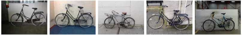
55 (a) Intact (b) Damaged (c) Absent (d) Occluded Figure 37: Examples of Back handles in the different states (a) Intact (b) Damaged (c) Absent (d) Occluded Figure 38: Examples of Back lights in the different states 54

56 (a) Intact (b) Damaged (c) Absent (d) Occluded Figure 39: Examples of Back mudguards in the different states (a) Intact (b) Damaged (c) Absent (d) Occluded Figure 40: Examples of Front wheels in the different states 55

57 (a) Intact (b) Damaged (c) Absent (d) Occluded Figure 41: Examples of Back wheels in the different states (a) Intact (b) Damaged (c) Absent (d) Occluded Figure 42: Examples of Front handbreaks in the different states 56

58 (a) Intact (b) Damaged (c) Absent (d) Occluded Figure 43: Examples of Front pedals in the different states (a) Intact (b) Damaged (c) Absent (d) Occluded Figure 44: Examples of Saddles in the different states 57

59 (a) Intact (b) Damaged (c) Absent (d) Occluded Figure 45: Examples of Bells in the different states (a) Intact (b) Damaged (c) Absent (d) Occluded Figure 46: Examples of Kickstands in the different states 58

60 (a) Intact (b) Damaged (c) Absent (d) Occluded Figure 47: Examples of Front handles in the different states (a) Intact (b) Damaged (c) Absent (d) Occluded Figure 48: Examples of Gear cases in the different states 59

61 (a) Intact (b) Damaged (c) Absent (d) Occluded Figure 49: Examples of Back reflectors in the different states (a) Intact (b) Damaged (c) Absent (d) Occluded Figure 50: Examples of Front lights in the different states 60

62 (a) Intact (b) Damaged (c) Absent (d) Occluded Figure 51: Examples of Chains in the different states (a) Intact (b) Damaged (c) Absent (d) Occluded Figure 52: Examples of Back pedals in the different states 61

63 (a) Intact (b) Damaged (c) Absent (d) Occluded Figure 53: Examples of Back hand breaks in the different states 62

64 D State coorelations Figure 54: Coorelation matrix for Intact vs Intact 63

65 Figure 55: Coorelation matrix for Intact vs Damaged 64

66 Figure 56: Coorelation matrix for Intact vs Absent 65

67 Figure 57: Coorelation matrix for Intact vs Occluded 66

68 Figure 58: Coorelation matrix for Damaged vs Intact 67

69 Figure 59: Coorelation matrix for Damaged vs Damaged 68

70 Figure 60: Coorelation matrix for Damaged vs Absent 69

71 Figure 61: Coorelation matrix for Damaged vs Occluded 70

72 Figure 62: Coorelation matrix for Absent vs Intact 71

73 Figure 63: Coorelation matrix for Absent vs Damaged 72

74 Figure 64: Coorelation matrix for Absent vs Absent 73

75 Figure 65: Coorelation matrix for Absent vs Occluded 74

76 Figure 66: Coorelation matrix for Occluded vs Intact 75

77 Figure 67: Coorelation matrix for Occluded vs Damaged 76

78 Figure 68: Coorelation matrix for Occluded vs Absent 77

79 Figure 69: Coorelation matrix for Occluded vs Occluded 78

80 E Average Bikes Figure 70: Mean of all images centered around the Back Handle. Figure 71: Mean of all images centered around the Back Hand Break. 79