Mesh generation using blockmesh. blockmesh

Transcription

1 Mesh generation using blockmesh blockmesh blockmesh is a multi-block mesh generator. For simple geometries, the mesh generation utility blockmesh can be used. The mesh is generated from a dictionary file named blockmeshdict located in the system directory. The meshing tool generates high quality meshes, it is the tool to use for very simple geometries. As the complexity of the geometry increases, the effort and time required to setup the dictionary increases a lot. Usually the background mesh used with snappyhexmesh consist of a single rectangular block, therefore blockmesh can be used with no problem. It is highly recommended to create a template of the dictionary blockmeshdict that you can change according to the dimensions of your domain. You can also use m4 or Python scripting to automate the whole process. 1

2 Mesh generation using blockmesh blockmesh 2

3 Mesh generation using blockmesh blockmesh workflow To generate a mesh with blockmesh, you will need to define the vertices, block connectivity and number of cells in each direction. To assign boundary patches, you will need to define the faces connectivity 3

4 Let us take a close look to a blockmeshdict dictionary. We will use the square cavity case. You will find this case in the directory: 101BLOCKMESH/C1 From this point on, please follow me. We are all going to work at the same pace. Remember, $PTOFC is pointing to the path where you unpacked the tutorials. 4

5 What are we going to do? We will use this simple case to take a close look at a blockmeshdict dictionary. We will study all sections in the blockmeshdict dictionary. We will introduce two features useful for parameterization, namely, macro syntax and inline calculations. You can use this dictionary as a blockmeshdict template that you can change automatically according to the dimensions of your domain and the desired cell spacing. 5

6 17 converttometers 1; xmin 0; 20 xmax 1; 21 ymin 0; 22 ymax 1; 23 zmin 0; 24 zmax 1; deltax 0.05; 31 deltay 0.05; 32 deltaz 0.05; lx #calc "$xmax - $xmin"; 35 ly #calc "$ymax - $ymin"; 36 lz #calc "$zmax $zmin"; xcells #calc "round($lx/$deltax)"; 39 ycells #calc "round($ly/$deltay)"; 40 zcells #calc "round($lz/$deltaz)"; vertices 45 ( 46 //BLOCK 0 47 ($xmin $ymin $zmin) //0 48 ($xmax $ymin $zmin) //1 49 ($xmax $ymax $zmin) //2 50 ($xmin $ymax $zmin) //3 51 ($xmin $ymin $zmax) //4 52 ($xmax $ymin $zmax) //5 53 ($xmax $ymax $zmax) //6 54 ($xmin $ymax $zmax) //7 66 ); The keyword converttometers (line 17), is a scaling factor. In this case we do not scale the dimensions. In lines we declare some variables using macro syntax notation. With macro syntax, we first declare the variables and their values (lines 19-24), and then we can use the variables by adding the symbol $ to the variable name (lines 47-54). In lines we use macro syntax to declare another set of variables that will be used later. Macro syntax is a very convenient way to parameterize dictionaries. 6

7 17 converttometers 1; xmin 0; 20 xmax 1; 21 ymin 0; 22 ymax 1; 23 zmin 0; 24 zmax 1; deltax 0.05; 31 deltay 0.05; 32 deltaz 0.05; lx #calc "$xmax - $xmin"; 35 ly #calc "$ymax - $ymin"; 36 lz #calc "$zmax $zmin"; xcells #calc "round($lx/$deltax)"; 39 ycells #calc "round($ly/$deltay)"; 40 zcells #calc "round($lz/$deltaz)"; vertices 45 ( 46 //BLOCK 0 47 ($xmin $ymin $zmin) //0 48 ($xmax $ymin $zmin) //1 49 ($xmax $ymax $zmin) //2 50 ($xmin $ymax $zmin) //3 51 ($xmin $ymin $zmax) //4 52 ($xmax $ymin $zmax) //5 53 ($xmax $ymax $zmax) //6 54 ($xmin $ymax $zmax) //7 66 ); In lines we are doing inline calculations using the directive #calc. Basically we are programming directly in the dictionary. OpenFOAM will compile this function as it reads it. With inline calculations and codestream you can access many OpenFOAM functions from the dictionaries. Inline calculations and codestream are very convenient ways to parameterize dictionaries and program directly on the dictionaries. 7

8 17 converttometers 1; xmin 0; 20 xmax 1; 21 ymin 0; 22 ymax 1; 23 zmin 0; 24 zmax 1; deltax 0.05; 31 deltay 0.05; 32 deltaz 0.05; lx #calc "$xmax - $xmin"; 35 ly #calc "$ymax - $ymin"; 36 lz #calc "$zmax $zmin"; xcells #calc "round($lx/$deltax)"; 39 ycells #calc "round($ly/$deltay)"; 40 zcells #calc "round($lz/$deltaz)"; vertices 45 ( 46 //BLOCK 0 47 ($xmin $ymin $zmin) //0 48 ($xmax $ymin $zmin) //1 49 ($xmax $ymax $zmin) //2 50 ($xmin $ymax $zmin) //3 51 ($xmin $ymin $zmax) //4 52 ($xmax $ymin $zmax) //5 53 ($xmax $ymax $zmax) //6 54 ($xmin $ymax $zmax) //7 66 ); To do inline calculations using the directive #calc, we proceed as follows (we will use line 35 as example): ly #calc "$ymax - $ymin"; We first give a name to the new variable (ly), we then tell OpenFOAM that we want to do an inline calculation (#calc), and then we do the inline calculation ("$ymax- $ymin";). Notice that the operation must be between double quotation marks. 8

9 17 converttometers 1; xmin 0; 20 xmax 1; 21 ymin 0; 22 ymax 1; 23 zmin 0; 24 zmax 1; deltax 0.05; 31 deltay 0.05; 32 deltaz 0.05; lx #calc "$xmax - $xmin"; 35 ly #calc "$ymax - $ymin"; 36 lz #calc "$zmax $zmin"; xcells #calc "round($lx/$deltax)"; 39 ycells #calc "round($ly/$deltay)"; 40 zcells #calc "round($lz/$deltaz)"; vertices 45 ( 46 //BLOCK 0 47 ($xmin $ymin $zmin) //0 48 ($xmax $ymin $zmin) //1 49 ($xmax $ymax $zmin) //2 50 ($xmin $ymax $zmin) //3 51 ($xmin $ymin $zmax) //4 52 ($xmax $ymin $zmax) //5 53 ($xmax $ymax $zmax) //6 54 ($xmin $ymax $zmax) //7 66 ); In lines lines 34-36, we use inline calculations to compute the length in each direction. Then we compute the number of cells to be used in each direction (lines 38-40). To compute the number of cells we use as cell spacing the values declared in lines By proceeding in this way, we can compute automatically the number of cells needed in each direction according to the desired cell spacing. 9

10 17 converttometers 1; xmin 0; 20 xmax 1; 21 ymin 0; 22 ymax 1; 23 zmin 0; 24 zmax 1; deltax 0.05; 31 deltay 0.05; 32 deltaz 0.05; lx #calc "$xmax - $xmin"; 35 ly #calc "$ymax - $ymin"; 36 lz #calc "$zmax $zmin"; xcells #calc "round($lx/$deltax)"; 39 ycells #calc "round($ly/$deltay)"; 40 zcells #calc "round($lz/$deltaz)"; vertices 45 ( 46 //BLOCK 0 47 ($xmin $ymin $zmin) //0 48 ($xmax $ymin $zmin) //1 49 ($xmax $ymax $zmin) //2 50 ($xmin $ymax $zmin) //3 51 ($xmin $ymin $zmax) //4 52 ($xmax $ymin $zmax) //5 53 ($xmax $ymax $zmax) //6 54 ($xmin $ymax $zmax) //7 66 ); By the way, as this dictionary is designed for blocks with positive vertices coordinates, there is a small catch in the way we compute the length (lines 34-36) and the number of cells (lines 38-40). What will happen if xmin is negative? What will happen if xcells is negative? What will happen if xcells is a float with decimals? Can you find a solution to these small problems? 10

11 17 converttometers 1; xmin 0; 20 xmax 1; 21 ymin 0; 22 ymax 1; 23 zmin 0; 24 zmax 1; deltax 0.05; 31 deltay 0.05; 32 deltaz 0.05; lx #calc "$xmax - $xmin"; 35 ly #calc "$ymax - $ymin"; 36 lz #calc "$zmax $zmin"; xcells #calc "round($lx/$deltax)"; 39 ycells #calc "round($ly/$deltay)"; 40 zcells #calc "round($lz/$deltaz)"; vertices 45 ( 46 //BLOCK 0 47 ($xmin $ymin $zmin) //0 48 ($xmax $ymin $zmin) //1 49 ($xmax $ymax $zmin) //2 50 ($xmin $ymax $zmin) //3 51 ($xmin $ymin $zmax) //4 52 ($xmax $ymin $zmax) //5 53 ($xmax $ymax $zmax) //6 54 ($xmin $ymax $zmax) //7 66 ); In the vertices section (lines 44-66), we define the vertex coordinates of the geometry. In this case, there are eight vertices defining a 3D block. Remember, OpenFOAM always uses 3D meshes, even if the simulation is 2D. For 2D meshes, you only add one cell in the third dimension. Notice that the vertex numbering starts from 0 (as the counters in c++). This numbering applies for blocks as well. 11

12 In lines 68-71, we define the block topology, hex means that it is a structured hexahedral block. In this case, we are generating a rectangular mesh. In line 70, ( ) are the vertices used to define the block (and yes, the order is important). Each hex block is defined by eight vertices, in sequential order. Where the first vertex in the list represents the origin of the coordinate system (vertex 0 in this case). ($xcells $ycells $zcells) is the number of mesh cells in each direction (X Y Z). Notice that we are using macro syntax, and we compute the values using inline calculations. simplegrading (1 1 1) is the grading or mesh stretching in each direction (X Y Z), in this case the mesh is uniform. We will deal with mesh grading/stretching in the next case. 68 blocks 69 ( 70 hex ( ) ($xcells $ycells $zcells) simplegrading (1 1 1) 71 ); edges 74 ( ); 12

13 Let us talk about the block ordering hex ( ), which is extremely important. hex blocks are defined by eight vertices in sequential order. Where the first vertex in the list represents the origin of the coordinate system (vertex 0 in this case). Starting from this vertex, we construct the block topology. So in this case, the first part of the block is made up by vertices and the second part of the block is made up by vertices (notice that we start from vertex 4 which is the projection in the Z-direction of vertex 0). In this case, the vertices are ordered in such a way that if we look at the screen/paper (-z direction), the vertices rotate counter-clockwise. If you add a second block, you must identify the first vertex and starting from it, you should construct the block topology. In this case, you might need to merges faces, we will address this later. 68 blocks 69 ( 70 hex ( ) ($xcells $ycells $zcells) simplegrading (1 1 1) 71 ); edges 74 ( ); 13

14 Edges, are constructed from the vertices definition. Each edge joining two vertices is assumed to be straight by default. The user can specified any edge to be curved by entries in the section edges. Possible options are: arc, spline, polyline, BSpline, line. For example, to define an arc we first define the vertices to be connected to form an edge and then we give an interpolation point. To define a polyline we first define the vertices to be connected to form an edge and then we give a list of the coordinates of the interpolation points. In this case and as we do not specified anything, all edges are assumed to be straight lines. 68 blocks 69 ( 70 hex ( ) ($xcells $ycells $zcells) simplegrading (1 1 1) 71 ); edges 74 ( ); 14

15 78 boundary 79 ( 80 top 81 { 82 type wall; 83 faces 84 ( 85 ( ) 86 ); 87 } 88 left 89 { 90 type wall; 91 faces 92 ( 93 ( ) 94 ); 95 } 96 right 97 { 98 type wall; 99 faces 100 ( 101 ( ) 102 ); 103 } 104 bottom 105 { 106 type wall; 107 faces 108 ( 109 ( ) 110 ); 111 } In the section boundary, we define all the patches where we want to apply boundary conditions. This step is of paramount importance, because if we do not define the surface patches we will not be able to apply the boundary conditions to individual surface patches. 15

16 78 boundary 79 ( 80 top 81 { 82 type wall; 83 faces 84 ( 85 ( ) 86 ); 87 } 88 left 89 { 90 type wall; 91 faces 92 ( 93 ( ) 94 ); 95 } 96 right 97 { 98 type wall; 99 faces 100 ( 101 ( ) 102 ); 103 } 104 bottom 105 { 106 type wall; 107 faces 108 ( 109 ( ) 110 ); 111 } In lines we define a boundary patch. In line 80 we define the patch name top (the name is given by the user). In line 82 we give a base type to the surface patch. In this case wall (do not worry we are going to talk about this later). In line 85 we give the connectivity list of the vertices that made up the surface patch or face, that is, ( ). Have in mind that the vertices need to be neighbors and it does not matter if the ordering is clockwise or counter clockwise. 16

17 78 boundary 79 ( 80 top 81 { 82 type wall; 83 faces 84 ( 85 ( ) 86 ); 87 } 88 left 89 { 90 type wall; 91 faces 92 ( 93 ( ) 94 ); 95 } 96 right 97 { 98 type wall; 99 faces 100 ( 101 ( ) 102 ); 103 } 104 bottom 105 { 106 type wall; 107 faces 108 ( 109 ( ) 110 ); 111 } Have in mind that the vertices need to be neighbors and it does not matter if the ordering is clockwise or counter clockwise. Remember, faces are defined by a list of 4 vertex numbers, e.g., ( ). In lines we define the patch left. In lines we define the patch right. In lines we define the patch bottom. 17

18 112 front 113 { 114 type wall; 115 faces 116 ( 117 ( ) 118 ); 119 } 120 back 121 { 122 type wall; 123 faces 124 ( 125 ( ) 126 ); 127 } 128 ); mergepatchpairs 131 ( ); In lines we define the patch front. In lines we define the patch back. You can also group many faces into one patch, for example, instead of creating the patches front and back, you can group them into a single patch named backandfront, as follows, backandfront { type wall; faces ( ( ) ( ) ); } 18

19 112 front 113 { 114 type wall; 115 faces 116 ( 117 ( ) 118 ); 119 } 120 back 121 { 122 type wall; 123 faces 124 ( 125 ( ) 126 ); 127 } 128 ); mergepatchpairs 131 ( ); We can merge blocks in the section mergepatchpairs (lines ). The block patches to be merged must be first defined in the boundary list, blockmesh then connect the two blocks. In this case, as we have one single block there is no need to merge patches. 19

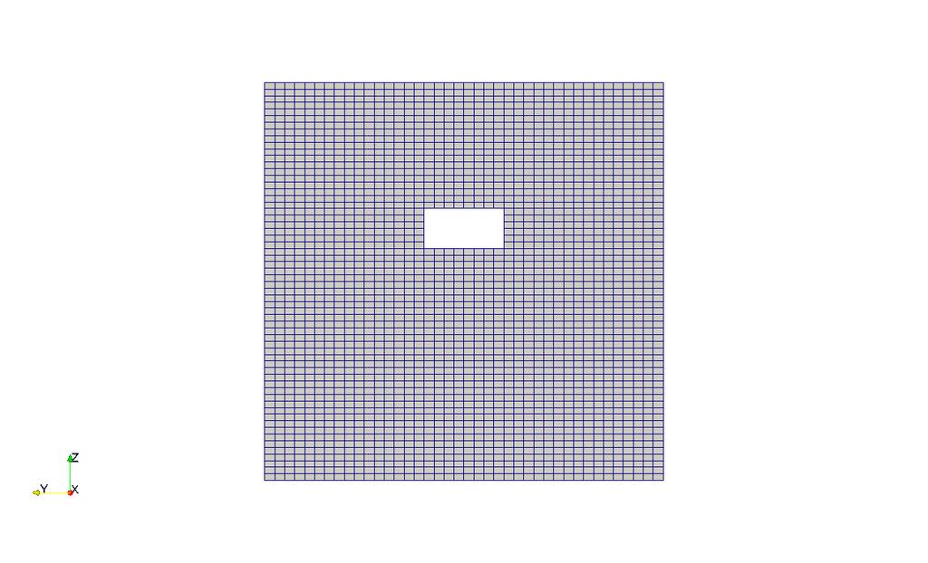
20 To sum up, the blockmeshdict dictionary generates a single block with: X/Y/Z dimensions: 1.0/1.0/1.0 As the cell spacing in all directions is defined as 0.05, it will use the following number of cells in the X, Y and Z directions: 20 x 20 x 20 cells. One single hex block with straight lines. Six patches of base type wall, namely, left, right, top, bottom, front and back. The information regarding the patch base type and patch name is saved in the file boundary. Feel free to modify this file to fit your needs. Remember to use the utility checkmesh to check the quality of the mesh and look for topological errors. Topological errors must be repaired. 20

21 ( 20 top 21 { 22 type wall; 23 ingroups 1(wall); 24 nfaces 400; 25 startface 22800; 26 } 27 left 28 { 29 type wall; 30 ingroups 1(wall); 31 nfaces 400; 32 startface 23200; 33 } 34 right 35 { 36 type empty; 37 ingroups 1(wall); 38 nfaces 400; 39 startface 23600; 40 } 41 bottom 42 { 43 type wall; 44 ingroups 1(wall); 45 nfaces 400; 46 startface 24000; 47 } 48 front 49 { 50 type wall; 51 ingroups 1(wall); 52 nfaces 400; 53 startface 24400; 54 } 55 back 56 { 57 type empty; 58 ingroups 1(wall); 59 nfaces 400; 60 startface 24800; 61 } 62 ) The constant/polymesh/boundary dictionary First at all, this file is automatically generated after you create the mesh or you convert it from a third party format. In this file, the geometrical information related to the base type patch of each boundary of the domain is specified. The base type boundary condition is the actual surface patch where we are going to apply a primitive type boundary condition (or numerical boundary condition). The primitive type boundary condition assign a field value to the surface patch (base type). You define the numerical type patch (or the value of the boundary condition), in the directory 0 or time directories. The name and base type of the patches was defined in the dictionary blockmeshdict in the section boundary. You can change the name if you do not like it. Do not use strange symbols or white spaces. You can also change the base type. For instance, you can change the type of the patch top from wall to patch. 21

22 ( 20 top 21 { 22 type wall; 23 ingroups 1(wall); 24 nfaces 400; 25 startface 22800; 26 } 27 left 28 { 29 type wall; 30 ingroups 1(wall); 31 nfaces 400; 32 startface 23200; 33 } 34 right 35 { 36 type empty; 37 ingroups 1(wall); 38 nfaces 400; 39 startface 23600; 40 } 41 bottom 42 { 43 type wall; 44 ingroups 1(wall); 45 nfaces 400; 46 startface 24000; 47 } 48 front 49 { 50 type wall; 51 ingroups 1(wall); 52 nfaces 400; 53 startface 24400; 54 } 55 back 56 { 57 type empty; 58 ingroups 1(wall); 59 nfaces 400; 60 startface 24800; 61 } 62 ) The constant/polymesh/boundary dictionary If you do not define the boundary patches in the dictionary blockmeshdict, they are grouped automatically in a default group named defaultfaces of type empty. For instance, if you do not assign a base type to the patch front, it will be grouped as follows: defaultfaces { type } empty; 1(empty); ingroups nfaces 400; startface 24800; Remember, you can manually change the name and type. 22

23 ( 20 top 21 { 22 type wall; 23 ingroups 1(wall); 24 nfaces 400; 25 startface 22800; 26 } 27 left 28 { 29 type wall; 30 ingroups 1(wall); 31 nfaces 400; 32 startface 23200; 33 } 34 right 35 { 36 type empty; 37 ingroups 1(wall); 38 nfaces 400; 39 startface 23600; 40 } 41 bottom 42 { 43 type wall; 44 ingroups 1(wall); 45 nfaces 400; 46 startface 24000; 47 } 48 front 49 { 50 type wall; 51 ingroups 1(wall); 52 nfaces 400; 53 startface 24400; 54 } 55 back 56 { 57 type empty; 58 ingroups 1(wall); 59 nfaces 400; 60 startface 24800; 61 } 62 ) The constant/polymesh/boundary dictionary Number of surface patches In the list bellow there must be 6 patches definition. left back top bottom front right 23

24 The constant/polymesh/boundary dictionary ( 20 top 21 { 22 type wall; 23 ingroups 1(wall); 24 nfaces 400; 25 startface 22800; 26 } 27 left 28 { 29 type wall; 30 ingroups 1(wall); 31 nfaces 400; 32 startface 23200; 33 } 34 right 35 { 36 type wall; 37 ingroups 1(wall); 38 nfaces 400; 39 startface 23600; 40 } 41 bottom 42 { 43 type wall; 44 ingroups 1(wall); 45 nfaces 400; 46 startface 24000; 47 } 48 front 49 { 50 type wall; 51 ingroups 1(wall); 52 nfaces 400; 53 startface 24400; 54 } 55 back 56 { 57 type wall; 58 ingroups 1(wall); 59 nfaces 400; 60 startface 24800; 61 } 62 ) Name and type of the surface patches The name and base type of the patch is given by the user. In this case the name and base type was assigned in the dictionary blockmeshdict. You can change the name if you do not like it. Do not use strange symbols or white spaces. You can also change the base type. For instance, you can change the type of the patch top from wall to patch. 24

25 The constant/polymesh/boundary dictionary ( 20 top 21 { 22 type wall; 23 ingroups 1(wall); 24 nfaces 400; 25 startface 22800; 26 } 27 left 28 { 29 type wall; 30 ingroups 1(wall); 31 nfaces 400; 32 startface 23200; 33 } 34 right 35 { 36 type wall; 37 ingroups 1(wall); 38 nfaces 400; 39 startface 23600; 40 } 41 bottom 42 { 43 type wall; 44 ingroups 1(wall); 45 nfaces 400; 46 startface 24000; 47 } 48 front 49 { 50 type wall; 51 ingroups 1(wall); 52 nfaces 400; 53 startface 24400; 54 } 55 back 56 { 57 type wall; 58 ingroups 1(wall); 59 nfaces 400; 60 startface 24800; 61 } 62 ) ingroups keyword This is optional. You can erase this information safely. It is used to group patches during visualization in ParaView/paraFoam. If you open this mesh in parafoam you will see that there are two groups, namely: wall and empty. As usual, you can change the name. If you want to put a surface patch in two groups, you can proceed as follows: 2(wall wall1) In this case the surface patch belongs to the group wall (which can have another patch) and the group wall1 25

26 The constant/polymesh/boundary dictionary ( 20 top 21 { 22 type wall; 23 ingroups 1(wall); 24 nfaces 400; 25 startface 22800; 26 } 27 left 28 { 29 type wall; 30 ingroups 1(wall); 31 nfaces 400; 32 startface 23200; 33 } 34 right 35 { 36 type wall; 37 ingroups 1(wall); 38 nfaces 400; 39 startface 23600; 40 } 41 bottom 42 { 43 type wall; 44 ingroups 1(wall); 45 nfaces 400; 46 startface 24000; 47 } 48 front 49 { 50 type wall; 51 ingroups 1(wall); 52 nfaces 400; 53 startface 24400; 54 } 55 back 56 { 57 type wall; 58 ingroups 1(wall); 59 nfaces 400; 60 startface 24800; 61 } 62 ) nfaces and startface keywords Unless you know what you are doing, you do not need to change this information. Basically, this is telling you the starting face and ending face of the patch. This information is created automatically when generating the mesh or converting the mesh. 26

27 Running the case To generate the mesh, in the terminal window type: 1. $> foamcleantutorials 2. $> blockmesh 4. $> checkmesh 5. $> parafoam 27

28 Let us take a close look to a blockmeshdict dictionary to study how to use mesh grading. We will use the square cavity case. You will find this case in the directory: 101BLOCKMESH/C2 From this point on, please follow me. We are all going to work at the same pace. Remember, $PTOFC is pointing to the path where you unpacked the tutorials. 28

29 What are we going to do? We will use this case to study how to change mesh grading (growth rate). You can use this dictionary as a blockmeshdict template that you can change automatically according to the dimensions of your domain and the desired cell spacing and growth rate. 29

30 No grading 61 blocks 62 ( 63 hex ( ) ($xcells $ycells $zcells) simplegrading (1 1 1) 88 ); Mesh grading To control mesh grading, we use the simplegrading keyword. Setting the values to (1 1 1) means no grading (uniform mesh). A value different from 1 will add grading to the edge, that is, it will cluster more cells towards one extreme of the block. Let us take a look at a 2D mesh. 30

31 Unidirectional grading Stretching in the Y direction (edge 0-3) 61 blocks 62 ( 63 hex ( ) ($xcells $ycells $zcells) simplegrading ( ) 88 ); Stretching in the X direction (edge 0-1) Unidirectional grading Stretching in the Y direction (edge 0-3) 61 blocks 62 ( 63 hex ( ) ($xcells $ycells $zcells) simplegrading (8 8 1) 88 ); Stretching in the X direction (edge 0-1) 31

32 Unidirectional grading Stretching in the Y direction (edge 0-3) 61 blocks 62 ( 63 hex ( ) ($xcells $ycells $zcells) simplegrading ( ) 88 ); Stretching in the X direction (edge 0-1) Unidirectional grading Stretching in the Y direction (edge 0-3) 61 blocks 62 ( 63 hex ( ) ($xcells $ycells $zcells) simplegrading ( ) 88 ); Stretching in the X direction (edge 0-1) 32

33 Multi-grading of a block Using a single grading to describe mesh grading permits only one-way grading of the block. For example, to mesh the square cavity with grading towards all the walls requires four blocks, each one with different grading. To reduce complexity and effort we can use multi-grading to control grading within separate divisions of a single block, rather than have to define several blocks with one grading per block. BLOCK 0 BLOCK 1 BLOCK 3 BLOCK 2 33

34 61 blocks 62 ( hex ( ) ($xcells $ycells $zcells) 66 simplegrading 67 ( 68 // x-direction expansion ratio 70 ( 71 ( ) //Division 1 72 ( ) //Division 2 73 ( ) //Division 3 74 ) // y-direction expansion ratio 78 ( 79 ( ) 80 ( ) 81 ( ) 82 ) // z-direction expansion ratio 85 1 //no expansion ratio 86 ) ); Multi-grading of a block Let us use multi-grading in the X-direction (lines 70-74). First, we split the block into 3 divisions in the X- direction representing 20% or 0.2 (division 1), 60% or 0.6 (division 2), and 20% or 0.2 (division 3) of the block length. Then, we assign 25% (0.25) of the total cells in the X- direction in divisions 1 and 3, and the remaining 50% (0.50) in division 2. Finally, we apply a grading of 8 in division 1, a grading of 1 (uniform mesh) in division 2, and a grading of(1/8) in division 3. 34

35 61 blocks 62 ( hex ( ) ($xcells $ycells $zcells) 66 simplegrading 67 ( 68 // x-direction expansion ratio 70 ( 71 ( ) 72 ( ) 73 ( ) 74 ) // y-direction expansion ratio 78 ( 79 ( ) //Division 1 80 ( ) //Division 2 81 ( ) //Division 3 82 ) // z-direction expansion ratio 85 1 //no expansion ratio 86 ) ); Multi-grading of a block Let us use multi-grading in the Y-direction (lines 78-82). First, we split the block into 3 divisions in the Y- direction representing 20% or 0.2 (division 1), 60% or 0.6 (division 2), and 20% or 0.2 (division 3) of the block length. Then, we assign 25% (0.25) of the total cells in the Y- direction in divisions 1 and 3, and the remaining 50% (0.50) in division 2. Finally, we apply a grading of 8 in division 1, a grading of 1 (uniform mesh) in division 2, and a grading of(1/8) in division 3. 35

36 61 blocks 62 ( hex ( ) ($xcells $ycells $zcells) 66 simplegrading 67 ( 68 // x-direction expansion ratio 70 ( 71 ( ) 72 ( ) 73 ( ) 74 ) // y-direction expansion ratio 78 ( 79 ( ) 80 ( ) 81 ( ) 82 ) // z-direction expansion ratio ) ); Multi-grading of a block Finally, as the mesh is 2D, we do not need to add grading in the Z-direction (line 85). 36

37 Running the case To generate the mesh, in the terminal window type: 1. $> foamcleantutorials 2. $> blockmesh 3. $> checkmesh 4. $> parafoam 37

38 Let us take a close look to a blockmeshdict dictionary to study how to create multiple blocks. We will use the square cavity case. You will find this case in the directory: 101BLOCKMESH/C3 From this point on, please follow me. We are all going to work at the same pace. Remember, $PTOFC is pointing to the path where you unpacked the tutorials. 38

39 What are we going to do? We will use this case to take a close look at a blockmeshdict dictionary. We will study how to work with multiple blocks. When working with multiples blocks, we need to deal with the common face between blocks. If we do not connect these blocks, blockmesh will create a boundary patch and we will need to assign a boundary condition to this patch. When we connect the blocks, blockmesh will create an internal face (therefore we do not need to assign a boundary condition to the face). There are two ways to connect blocks, using face matching and face merging. Hereafter we are going to study face merging. 39

40 19 xmin 0; 20 xmax 1; 21 ymin 0.5; 22 ymax 1; 23 zmin 0; 24 zmax 1; ymin2 0; 27 ymax2 0.5; xcells 20; 30 ycells 10; 31 zcells 1; vertices 41 ( 42 //BLOCK 0 43 ($xmin $ymin $zmin) //0 44 ($xmax $ymin $zmin) //1 45 ($xmax $ymax $zmin) //2 46 ($xmin $ymax $zmin) //3 47 ($xmin $ymin $zmax) //4 48 ($xmax $ymin $zmax) //5 49 ($xmax $ymax $zmax) //6 50 ($xmin $ymax $zmax) // //BLOCK 1 53 ($xmin $ymin2 $zmin) //8 54 ($xmax $ymin2 $zmin) //9 55 ($xmax $ymax2 $zmin) //10 56 ($xmin $ymax2 $zmin) //11 57 ($xmin $ymin2 $zmax) //12 58 ($xmax $ymin2 $zmax) //13 59 ($xmax $ymax2 $zmax) //14 60 ($xmin $ymax2 $zmax) //15 71 ); Multiple blocks Face merging To do a mesh with multiple blocks we proceed in the same as we have done so far. When using face merging we need to define all the vertices that made up each block. In lines we use macro syntax to declare the variables that we will use to define the vertices. In lines we use macro syntax to define the number of cells in each direction. As this is a 2D case there is only one cell in the Z-direction. In lines we use macro syntax to define the vertices that made up each block. 40

41 73 blocks 74 ( 75 hex ( ) ($xcells $ycells $zcells) simplegrading (1 1 1) //BLOCK 0 76 hex ( ) ($xcells $ycells $zcells) simplegrading (1 1 1) //BLOCK 1 77 //hex ( ) (40 $ycells $zcells) simplegrading (1 1 1) 78 ); Multiple blocks Face merging In lines 73-78, we define the blocks. In line 75, ( ) are the vertices used to define block 0 (the top block). Remember, the first vertex in the list represents the origin of the coordinate system (vertex 0 in this case). Starting from this vertex, we construct the block topology. So in this case, the first part of the block is made up by vertices and the second part of the block is made up by vertices (notice that we start from vertex 4 which is the projection in the Z-direction of vertex 0). ($xcells $ycells $zcells) is the number of mesh cells in each direction (X Y Z). Notice that we are using macro syntax. simplegrading (1 1 1) is the grading or mesh stretching in each direction (X Y Z), in this case the mesh is uniform. 41

42 73 blocks 74 ( 75 hex ( ) ($xcells $ycells $zcells) simplegrading (1 1 1) //BLOCK 0 76 hex ( ) ($xcells $ycells $zcells) simplegrading (1 1 1) //BLOCK 1 77 //hex ( ) (40 $ycells $zcells) simplegrading (1 1 1) 78 ); Multiple blocks Face merging In line 76, ( ) are the vertices used to define block 1 (the bottom block). The first vertex in the list represents the origin of the coordinate system (vertex 8 in this case). Starting from this vertex, we construct the block topology. So in this case, the first part of the block is made up by vertices and the second part of the block is made up by vertices (notice that we start from vertex 12 which is the projection in the Z-direction of vertex 8). ($xcells $ycells $zcells) is the number of mesh cells in each direction (X Y Z). Notice that we are using macro syntax. simplegrading (1 1 1) is the grading or mesh stretching in each direction (X Y Z), in this case the mesh is uniform. 42

43 86 boundary 87 ( 88 movingwall 89 { 90 type wall; 91 faces 92 ( 93 ( ) 94 ); 95 } 96 fixedwalls 97 { 98 type wall; 99 faces 100 ( 101 ( ) 102 ( ) 104 ( ) 105 ( ) 106 ( ) 107 ); 108 } 131 back 132 { 133 type empty; 134 faces 135 ( 136 ( ) 137 ( ) 138 ); 139 } Multiple blocks Face merging In lines we define the boundary patches of the domain. We are defining the external patches. 43

44 141 interface1 142 { 143 type wall; 144 faces 145 ( 146 ( ) 147 ); 148 } interface2 151 { 152 type wall; 153 faces 154 ( 155 ( ) 156 ); 157 } 158 ); mergepatchpairs 161 ( 162 (interface1 interface2) 163 ); Multiple blocks Face merging In lines we define the boundary patches common to each block. In this case we need to use mergepatchpairs to create an internal face, otherwise OpenFOAM will see this patch as an boundary patch. To merge patches we need to define them in the section boundary of the blockmeshdict dictionary. In line 162 we merge the patches. The first entry corresponds to the master patch and the second entry is the slave patch. Master Slave 44

45 Multiple blocks Face merging The advantage of using face merging instead of face matching, is that we can use blocks with different grading and number of cells. If the blocks are different, blockmesh will modify the block that owns the slave patch in order to have a conforming mesh. The block that owns the master patch remains unchanged. 45

46 Running the case To generate the mesh, in the terminal window type: 1. $> foamcleantutorials 2. $> blockmesh 3. $> checkmesh 4. $> parafoam 46

47 73 blocks 74 ( 75 hex ( ) ($xcells $ycells $zcells) simplegrading (1 1 1) //BLOCK 0 76 //hex ( ) ($xcells $ycells $zcells) simplegrading (1 1 1) 77 hex ( ) (40 $ycells $zcells) simplegrading (1 1 1) //BLOCK 1 78 ); Multiple blocks Face merging To have different blocks, we changed the number of cells in the X-direction of the bottom block (line 77). The definition of the block topology remains unchanged, i.e., ( ). Also, the grading does not change. If you want you can use a non-uniform grading. Have in mind that the mesh will no longer be 2D because blockmesh will add cells to make the blocks conforming. To get the 2D mesh, you will need to use the utility extrudemesh, which reads the extrudemeshdict dictionary. Type in the terminal, $> extrudemesh 47

48 The extrudemeshdict dictionary. The utility extrudemesh will create a 2D mesh by projecting the source patch into the exposed patch. To create the 2D mesh, you will need to use 1 layer (nlayers). It is also recommended to set the extrusion thickness to constructfrom patch; sourcecase. 21 sourcepatches (back); exposedpatchname front; extrudemodel linearnormal nlayers 1; linearnormalcoeffs 32 { 33 thickness 1; 34 } mergefaces false; Name of source patch Name of the mirror patch Number of layers to use in the linear extrusion. As this is a 2D case we must use 1 layer Thickness of the extrusion. It is highly recommended to use a value of 1 48

49 Let us take a close look to a blockmeshdict dictionary to study how to create multiple blocks. We will use the square cavity case. You will find this case in the directory: 101BLOCKMESH/C4 From this point on, please follow me. We are all going to work at the same pace. Remember, $PTOFC is pointing to the path where you unpacked the tutorials. 49

50 What are we going to do? We will use this case to take a close look at a blockmeshdict dictionary. We will study how to work with multiple blocks. When working with multiples blocks, we need to deal with the common face between blocks. If we do not connect these blocks, blockmesh will create a boundary patch and we will need to assign a boundary condition. When we connect the blocks, blockmesh will create an internal face (therefore we do not need to assign a boundary condition to the face). There are two ways to connect blocks, using face matching and face merging. Hereafter we are going to study face matching. 50

51 19 xmin 0; 20 xmax 1; 21 ymin 0.5; 22 ymax 1; 23 zmin 0; 24 zmax 1; ymin2 0; 27 ymax2 0.5; xcells 20; 30 ycells 10; 31 zcells 1; vertices 41 ( 42 //BLOCK 0 43 ($xmin $ymin $zmin) //0 44 ($xmax $ymin $zmin) //1 45 ($xmax $ymax $zmin) //2 46 ($xmin $ymax $zmin) //3 47 ($xmin $ymin $zmax) //4 48 ($xmax $ymin $zmax) //5 49 ($xmax $ymax $zmax) //6 50 ($xmin $ymax $zmax) // //BLOCK 1 53 ($xmin $ymin2 $zmin) //8 54 ($xmax $ymin2 $zmin) //9 55 ($xmin $ymin2 $zmax) //10 56 ($xmax $ymin2 $zmax) //11 68 ); 138 mergepatchpairs 139 ( ); Multiple blocks Face matching To do a mesh with multiple blocks we proceed in the same way as we have done so far. When using face matching we do not need to define all the vertices that made up each block. For the common face between blocks, we only need to define one set of vertices. In lines we use macro syntax to declare the variables that we will use to define the vertices. In lines we use macro syntax to define the number of cells in each direction. As this is a 2D case there is only one cell in the Z-direction. 51

52 19 xmin 0; 20 xmax 1; 21 ymin 0.5; 22 ymax 1; 23 zmin 0; 24 zmax 1; ymin2 0; 27 ymax2 0.5; xcells 20; 30 ycells 10; 31 zcells 1; vertices 41 ( 42 //BLOCK 0 43 ($xmin $ymin $zmin) //0 44 ($xmax $ymin $zmin) //1 45 ($xmax $ymax $zmin) //2 46 ($xmin $ymax $zmin) //3 47 ($xmin $ymin $zmax) //4 48 ($xmax $ymin $zmax) //5 49 ($xmax $ymax $zmax) //6 50 ($xmin $ymax $zmax) // //BLOCK 1 53 ($xmin $ymin2 $zmin) //8 54 ($xmax $ymin2 $zmin) //9 55 ($xmin $ymin2 $zmax) //10 56 ($xmax $ymin2 $zmax) //11 68 ); 138 mergepatchpairs 139 ( ); Multiple blocks Face matching In lines we use macro syntax to define the vertices that made up each block. In lines we define the vertices that made up the top block. In lines we define the vertices that made up the bottom block. Notice that we are only defining the new vertices ( ). The vertices ( ), that are common between the block are not redefined. 52

53 Multiple blocks Face matching Have in mind that the blocks need to be identical, that is, same number of cells and same grading. If the blocks are different, blockmesh will not generate the mesh. You do not need to define the common patches in the section boundary of the blockmeshdict dictionary. Finally, we do not need to define the patches in the keyword mergepatchpairs as blockmesh will automatically merge the common faces. 53

54 Running the case To generate the mesh, in the terminal window type: 1. $> foamcleantutorials 2. $> blockmesh 3. $> checkmesh 4. $> parafoam 54

55 Let us take a close look to a blockmeshdict dictionary to study how to create non-straight edges. We will use the square cavity case. You will find this case in the directory: 101BLOCKMESH/C5 From this point on, please follow me. We are all going to work at the same pace. Remember, $PTOFC is pointing to the path where you unpacked the tutorials. 55

56 What are we going to do? We will use this case to take a close look at a blockmeshdict dictionary. We will study how to create non straight edges. Possible options are: arc, spline, polyline, Bspline, line. Edges are constructed from the vertices definition. Each edge joining two vertices is assumed to be straight by default. The user can specified any edge to be curved by entries in the section edges. For example, to define an arc we first define the vertices to be connected to form an edge and then we give an interpolation point. To define a polyline we first define the vertices to be connected to form an edge and then we give a list of the coordinates of the interpolation points. Let us study how to create curved edges using the square cavity case with face merging. 56

57 Interpolation method 70 edges 71 ( 107 spline ( 109 ( ) 110 ( ) 111 ( ) 112 ) 113 spline ( 115 ( ) 116 ( ) 117 ( ) 118 ) 119 spline ( 121 ( ) 122 ( ) 123 ( ) 124 ) 125 spline ( 127 ( ) 128 ( ) 129 ( ) 130 ) 133 ); Vertices to connect Interpolation points In lines we define spline edges. As we are using face merging, we need to define the splines in each common patch. To define a spline we first define the vertices to be connected to form an edge and then we give a list of the coordinates of the interpolation points. In lines we define the splines belonging to block 0. In lines we define the splines belonging to block 1. 57

58 Interpolation method Interpolation points 70 edges 71 ( 73 arc 0 1 ( ) 74 arc 4 5 ( ) 75 arc ( ) 76 arc ( ) 133 ); In lines we define arc edges. As we are using face merging, we need to define the arcs in each common patch. To define an arc we first define the vertices to be connected to form an edge and then we give an interpolation point. In lines we define the arcs belonging to block 0. In lines we define the arcs belonging to block 1. Vertices to connect 58

59 Running the case Choose any of the previous cases. To generate the mesh, in the terminal window type: 1. $> foamcleantutorials 2. $> blockmesh 3. $> checkmesh 4. $> parafoam 59

60 Let us take a close look to a blockmeshdict dictionary to study how to create an O-grid mesh. We will use the square cavity case. You will find this case in the directory: 101BLOCKMESH/C6 From this point on, please follow me. We are all going to work at the same pace. Remember, $PTOFC is pointing to the path where you unpacked the tutorials. 60

61 What are we going to do? We will use this case to take a close look at a blockmeshdict dictionary. We will create a 3D pipe using an O-grid topology. To create the O-grid topology we will use five blocks. At a first glance, this seems to be an easy task but it requires some work to layout the topology. We will use face matching. 61

62 17 converttometers 0.025; vertices 20 ( 21 //block0 vertices 22 ( ) //0 23 ( ) //1 24 ( ) //2 25 ( ) //3 26 ( ) //4 27 ( ) //5 28 ( ) //6 29 ( ) // //block1 new vertices 32 ( ) //8 33 ( ) //9 34 ( ) //10 35 ( ) // //block3 new vertices 38 ( ) //12 39 ( ) //13 40 ( ) //14 41 ( ) //15 42 ); xcells 20; 46 ycells 40; 47 zcells 60; xcells1 20; 50 ycells1 20; 51 zcells1 60; stretch 0.25; In this case we use and scaling factor of (line 17). We can also scale the mesh using the mesh utility transformpoints. In lines we define the coordinates of all the vertices. Remember, we are using face matching. In lines we use macro syntax to declare a set of variables that will be used later. 62

63 54 55 blocks 56 ( 57 //block0 58 hex ( ) ($xcells $ycells $zcells) simplegrading (1 $stretch 1) 59 //block1 60 hex ( ) ($xcells $ycells $zcells) simplegrading (1 $stretch 1) 61 //block2 62 hex ( ) ($xcells $ycells $zcells) simplegrading (1 $stretch 1) 63 //block3 64 hex ( ) ($xcells $ycells $zcells) simplegrading (1 $stretch 1) 65 //block4 66 hex ( ) ($xcells1 $ycells1 $zcells1) simplegrading (1 1 1) 67 ); In lines 55-67, we define all the blocks that made up the O-grid topology. Notice that we are creating five blocks. We also define the number of cells of each block and the grading. As we are using face matching, the grading and number of cells in the common faces need to be the same. 63

64 69 edges 70 ( 71 //block0 arc 72 arc 1 2 (0 1 0) 73 arc 5 6 ( ) //block1 arc 76 arc 2 9 (1 0 0) 77 arc 6 11 ( ) //block2 arc 80 arc 9 13 (0-1 0) 81 arc ( ) //block3 arc 84 arc 1 13 (-1 0 0) 85 arc 5 15 ( ) 86 ); boundary 89 ( inlet 92 { 93 type patch; 94 faces 95 ( 96 ( ) 97 ( ) 98 ( ) 99 ( ) 100 ( ) 101 ); 102 } 103 In lines we define arc edges. In lines we define the boundary patches. In lines we define the patch inlet. Notice that this boundary patch has five faces. 64

65 104 outlet 105 { 106 type patch; 107 faces 108 ( 109 ( ) 110 ( ) 111 ( ) 112 ( ) 113 ( ) 114 ); 115 } pipe 118 { 119 type wall; 120 faces 121 ( 122 ( ) 123 ( ) 124 ( ) 125 ( ) 126 ); 127 } ); mergepatchpairs 132 ( 133 ); In lines we define the boundary patches. In lines we define the patch outlet. Notice that this boundary patch has five faces. In lines we define the patch pipe. Notice that this boundary patch has four faces. In this case we do not use face merging (lines ). 65

66 Running the case To generate the mesh, in the terminal window type: 1. $> foamcleantutorials 2. $> blockmesh 3. $> checkmesh 4. $> parafoam 3D pipe O-grid topology (outlet patch) 66