SDG Cut: 3D Reconstruction of Non-lambertian Objects Using Graph Cuts on Surface Distance Grid

Transcription

1 SDG Cut: 3D Reconstruction of Non-lambertian Objects Using Graph Cuts on Surface Distance Grid Tianli Yu and Narendra Ahuja Beckman Institute & ECE Department Univ. of Illinois at Urbana-Champaign Urbana, IL Wei-Chao Chen Nvidia Corporation 2701 San Tomas Expressway Santa Clara, CA Abstract We show that the approaches to 3D reconstruction that use volumetric graph cuts to minimize a cost function over the object surface have two types of biases, the minimal surface bias and the discretization bias. These biases make it difficult to recover surface extrusions and other details, especially when a non-lambertian photo-consistency measure is used. To reduce these biases, we propose a new iterative graph cuts based algorithm that operates on the Surface Distance Grid (SDG), which is a special discretization of the 3D space, constructed using a signed distance transform of the current surface estimate. It can be shown that SDG significantly reduces the minimal surface bias, and transforms the discretization bias into a controllable degree of surface smoothness. Experiments on 3D reconstruction of non-lambertian objects confirm the effectiveness of our algorithm over previous methods. 1 Introduction Many multiple view 3D reconstruction methods are formulated as energy minimization problems [4, 7], which try to minimize the surface integral of a certain cost function. This formulation sets a generic framework where different minimization techniques can be applied. Under this framework, global optimization methods such as graph cuts can achieve a high quality reconstruction [14, 15]. However, this formulation and its discrete implementations using graph cuts have structural biases, e.g., certain types of surfaces are more likely to be selected as the optimal surface. These biases are more noticeable on noisy cost functions, such as those based on the non-lambertian photoconsistency measure [7]. These biases limit the algorithm s The support of the National Science Foundation under grant NSF IBN is gratefully acknowledged. Tianli Yu is now with the Embeded Imaging System Group of Motorola Labs. Contact: tianli.yu@motorola.com capability to recover surface details and extrusions. In this paper, we analyze the two types of biases of previous methods, and propose a method that we call the Graph Cuts on Surface Distance Grid, which is formulated in discrete domain and significantly reduces these biases. According to how 3D shape is represented, reconstruction methods can be roughly divided into two categories: those represented as a depth image and those represented as a 2D surface embedded in 3D space. Depth image representation is mostly used for small number of views, and has received extensive attention [11, 8]. The surface representation allows more accurate visibility reasoning and is more suitable to handle datasets with large numbers of views. These methods include voxel coloring/space carving [12, 9, 16], variational/level set methods [4, 7, 13] and graph cuts [14, 15]. The classic voxel coloring/space carving approaches suffer from the hard decisions of voxel removal at each step that affect the subsequent reconstructions. Energy minimization formulation in level set or graph cuts based methods postpones these hard decisions so that a trade-off can be made with respect to the entire surface. Level set methods embed the minimization of the surface integral into the evolution of the level set of a 3D function, which also handles topological changes. Graph cuts based methods approximate the surface integral using a discrete cost function defined on a regular 3D grid and a globally optimal result can be obtained via s-t min-cut algorithm [2]. As shown in Section 2, both of these methods have biases toward certain types of surfaces. Our paper is also related to the 3D reconstruction of nonlambertian objects which pose a significant challenge to many algorithms. Different approaches such as photometric stereo [6, 5], photometric stereo combined with multiple views [3], shape from shading [10] and Helmholtz Stereopsis [17] have been proposed. These methods usually make strong assumptions about the illumination and/or surface reflectance. For a more generic photo-consistency measure, Yang et al. [16] propose LMF (Line-Model-Fitting), which imposes the constraint that pixels from the same surface

2 point should form a line in RGB color space. But this measure requires known illumination color. Our paper modifies the photo-consistency measure proposed by Jin et al. [7], which is a rank constraint on the radiance matrix formed by neighboring surface points. This measure does not require illumination or surface reflectance to be known and therefore can be applied in more situations. It, however, has surface shape and texture dependent fluctuations which amplify the structural bias problems of the reconstruction. Soatto et al. [13] propose to partially solve the bias problem by using the integral of the cost function over the input images instead of the object surface. In this paper, we propose a new discrete formulation to alleviate these biases. This paper is organized as follows. We first discuss two types of structural bias for 3D reconstruction using graph cuts on regular volume grids (Sec. 2). Then we propose the Surface Distance Grid (SDG) and our discrete formulation of the reconstruction problem (Sec. 3). We present experiments on two real datasets to show the advantages of our algorithm (Sec. 4). Finally, we present conclusions and future research directions. 2 Structural Biases of Graph Cuts on Regular Volume Grid In the recently proposed Graph Cuts based methods for 3D reconstruction [15, 14] or volume segmentation [1], the problem is formulated as minimizing a surface integral of certain photo-consistency measure inside a search volume. A discrete 3D grid is constructed whose cut is used to approximate the surface integral. A global minimum is found using the s-t min-cut algorithm [2]. However, there are two structural bias problems associated with these methods. 2.1 Minimal Surface Bias The formulation of 3D reconstruction as minimizing a surface integral has an intrinsic bias toward surfaces with smaller area. This can be shown from the cost function: C(Γ) = M(x, n)da (1) Γ where M is the photo-consistency measure at each location x and local surface orientation n. The cost function C(Γ) is the surface integral of M. Clearly, for two surfaces with the same nonzero average photo-consistency M, the surface with smaller area will have smaller total cost. This bias can be neglected only when M is close to zero on the optimal surface, since the integral of zero on any surface is still zero. This bias is not restricted to graph cut based methods. Any method that uses this minimal surface integral formulation (such as the level set based methods) will have the same problem. Sometimes this property is used to regularize the C (a) A B F (b) Figure 1. Deviation from Euclidean Distance for Edge Cut and Node Cut algorithms. (a) E-Cut: D Euclid : AB=4, ACB= =7.21, D City : AB=4, ACB=9 (note the double counted edge near C). Bias toward AB (b) N-Cut: D Euclid : DF=4 2=5.66, DEF=8, D Chess : DF=4, DEF=8. Bias toward DF. solution by adding a positive offset to M, which will bias the surface toward smaller overall area to reduce noise. The mean curvature based flow in level set methods is an example [7]. On the other hand, this bias will try to cut out sharp corners or extrusions, as observed by Vogiatzis et al. [14]. In real applications, various noises or imperfections of the consistency model almost always make M shift from zero on the true surface, and therefore create an effective regularization offset. We will show an example of the non-lambertian photo-consistency measure in Section 4.1. Soatto et al. [13] propose to integrate the consistency measure over all the input images instead of on the object surface to reduce this bias. Their approach shows some improvement, but still has the bias toward surfaces with smaller silhouette area on the input images. This problem is also more prominent when graph cuts are used, since a global optimal solution is reached in the search space independent of the initial condition. A balloon force is used in [14] to prevent Graph Cuts from taking shortcuts, but at the risk of inflating the concave regions. 2.2 Discretization Bias The second type of bias comes from the approximation of the continuous integral in (1) by a discrete cost function. Volumetric graph cut methods construct a graph G = (V, E) based on a regular volume grid. Depending on the implementation, the photo-consistency measure can be put as the weights of edges E [14, 1] or nodes/vertices V [15]. We refer to these two type of methods as Edge Cut and Node Cut methods, respectively. The cost function is approximated by the cost of a cut, which is the summation of edge/node weights to be removed in order to partition the graph into two subgraphs S (connected to source s) and T (connected to sink t). For Edge Cut, the cost function is D E

3 Cost Function Search Range T S Distance to origin x (a) (b) (c) (d) (e) Figure 2. Discretization bias for Edge Cut and Node Cut reconstruction algorithms. (a) The cost function M 1 = ( x 0.6) 2 + d offset plotted with respect to the distance to the origin (center of the sphere). (b) Optimal surface by Edge Cut with d offset = 0. (c) Optimal surface by Edge Cut with d offset = Recovered surface shows bias that is parallel to the grid. (d) Optimal surface by Node Cut with d offset = 0. (e) Optimal surface by Node Cut with d offset = Recovered surface shows bias that is diagonal to the grid. C 1 (S, T ) = u S,v T,(u,v) E For Node Cut, the cost function is C 2 (S, T ) = v / S,v / T,v V c 1 (u, v) (2) c 2 (v) (3) where c 1 (u, v) is the weight of edge e uv, and c 2 (v) is the weight of node v. Boykov and Kolmogorov [1] discuss the optimal weight assignment for Edge Cut algorithms to approximate the surface integral in Euclidean space. They show that both a larger neighborhood system and a smaller grid size are needed in order to better approximate the integral. Due to various implementation reasons, recent volumetric graph cut methods often use the minimum 6-neighbor connectivity, which has very strong bias. For the 6-neighbor connectivity, the approximated distance for Edge Cut is the City Block Distance (4), and for Node Cut it is the Chessboard Distance (5): D City = x 2 x 1 + y 2 y 1 + z 2 z 1 (4) D Chess = max( x 2 x 1, y 2 y 1, z 2 z 1 ) (5) Fig.1 shows two examples of deviations from euclidean distance for 2D cases. In an edge capacitated graph (a), D City for AB is equal to D Euclid, but for ACB, D City is greater than D Euclid. This effectively gives a bias toward cuts that are parallel to the volume grid. Similarly, a node capacitated graph (b) results in a bias toward cuts that are diagonal to the volume grid. This bias becomes stronger if the minimum of the cost function is away from zero. The effects of the discretization biases on 3D reconstruction can be further illustrated in the following simulation. We use an isotropic cost function M 1 (x) = ( x 0.6) 2 + d offset (6) in a working volume (x, y, z) [ 1, 1] (Fig.2a). Where x is the distance from x to the origin. d offset is a parameter used to control the regularization offset. Clearly, M 1 reaches its minimum at the sphere surface x = 0.6. We build a grid with 6-neighbor connectivity and assign each edge (or node) the value of M 1 at that location. We use the s-t min-cut algorithm [2] to find the optimal Edge Cut (or Node Cut) that minimizes the total cost defined in (2) (or (3)) 1. For both algorithms, all the nodes with norm x < 0.3 are connected to the sink node t, and those with norm x > 0.9 are connected to the source node s. The ideal result for the continuous case is a sphere with a radius around The result for the two algorithms with different d offset values are shown in Fig.2. For d offset = 0 both algorithms obtain a nice approximation of the sphere. But with a slight increase of d offset, the discretization bias effect for the two algorithms becomes clearly visible. The artifacts are strong enough to remove many surface details in the reconstructed shape. Note that these biases can only be reduced by using both a larger neighborhood and a denser grid at the same time, which will significantly increase the graph complexity 3. 3 Graph Cuts on Surface Distance Grid To deal with the two types of biases, we propose the Graph Cuts on Surface Distance Grid algorithm, or SDG Cut. It is formulated as finding the minimum of a discrete cost function defined on the Surface Distance Grid (SDG). 1 For Node Cut, the graph has to be converted to another edge capacitated graph before minimization [15]. 2 Due to the minimal surface bias, the optimal surface is a sphere with radius smaller than 0.6 when d offset 0 3 The graph complexity can be estimated as O[(n m) 3 ] where n is the number of nodes in one dimension and m is the m-ring neighborhood.

4 Vertex Trajectories t Sink Node Initial Surface Candidate Points Add horizontal edges for smoothness Figure 3. Left: The initial surface of a fish sculpture constructed by silhouette cone intersection. Right: The inner most layer of the Surface Distance Grid (shaded surface) and the vertex trajectories from a dilated initial surface (colored lines). For better visualization, only 1/3 of the trajectories are shown. 3.1 Surface Distance Grid Surface Distance Grid is constructed from the signed distance transform of an initial surface. The signed distance transform D Γ (x) : R 3 R of a surface Γ is defined as: { min D Γ (x) = p Γ x p, if x is outside Γ min p Γ x p, if x is inside Γ (7) where is the L 2 norm and p is a point on the surface Γ. The steps in constructing a SDG are as follows: a. Start with an initial surface Γ 0. Compute its signed distance transform D Γ0 (x) inside a working volume. b. Choose an initial distance d 1 0 and extract a triangular mesh G 1 = (V 1, E 1 ) from the level set D Γ0 (x) = d 1, whose vertices are V 1 and edges are E 1. G 1 is used as the outermost layer of the SDG. c. Consider each vertex v in V 1, move it along the negative gradient of D Γ0 (x), and place k points at a spacing of d on the moving trajectory. These are the candidate points for v in the search space. The candidate points of all vertices form the Surface Distance Grid. d. At each candidate point, a photo-consistency measure is computed. If a normal is needed for the computation, it can be approximated by the gradient of D Γ0 (x) at that location. Clearly, as long as d 1 k d < 0, the SDG will be a k + 1 layer point cloud that occupies a dilated band around the initial surface Γ 0. Fig. 3 shows an example of vertex trajectories we created from an initial surface D reconstruction using Graph Cuts on SDG For each vertex in V 1, we want to select one corresponding candidate point, such that the sum of photo-consistency Surface Distance Grid Candidate points map to vertical edges s Source Node Figure 4. Converting a Surface Distance Grid to an edge capacitated graph G 2 to find the optimal subset of candidate points. measure of selected candidate points is minimized. We compute this optimal subset of candidate points by applying the s-t min-cut algorithm on an edge capacitated graph G 2, with each edge corresponding to a candidate point and each vertex representing the link between consecutive candidate points on the trajectory (Fig.4). These edges are called vertical edges and their weights We V are the photo-consistency measures of the corresponding candidate points. There are also vertices at two ends of each trajectory with infinite-weight edges to the source s and sink t. With only vertical edges, a minimum cut on G 2 can actually be obtained by choosing the minimum weight edge for each trajectory. There are no interactions between neighboring trajectories in this case. To impose certain smoothness constraint, we add horizontal edges to each layer of vertices in G 2, with the same connectivity as the original mesh G 1. Fig.4 illustrates the whole conversion process. The weight Wu,v H of a horizontal edge with u and v as two end nodes is: W H u,v = (W N u + W N v ) l 0 /L uv (8) W N u = (W V a + W V b )/2, W N v = (W V c + W V d )/2 (9) where a, b are two vertical edges connected to u and c, d are two vertical edges connected to v. L uv is the length of the corresponding edge uv in the mesh G 1. In (8), the horizontal weight W H u,v is set to be inversely proportional to L uv so that longer edges in G 1 are easier to cut. This is because the vertices of longer edges are further apart and less likely to be in the same layer. l 0 is an adjustable constant that controls the amount of regularization we want to apply. The larger l 0 is, the higher the cost for a cut to jump from one layer to another. This regularization tries to make the resultant surface remain parallel to the initial surface. Our problem can now be formulated as that of finding a cut that can separate G 2 into two subgraphs S (connected to source s) and T (connected to sink t), and minimize the

5 Initial Surface Compute the Signed Distance Transform Construct the Surface Distance Grid Compute the outermost triangular mesh G1 Cut 2 Reconstructed Surface Convert the result to a new surface Multiple Iterations Determine visibilities of vertices in G1 Cut 1 Graph Cut optimization on G2 Construct edge capacitated graph G2 Compute photo consistency values of candidate points Figure 5. Overview of the graph cuts on Surface Distance Grid reconstruction algorithm. Figure 6. A 2D example of different cuts on SDG. Although Cut 1 and Cut 2 have different euclidean lengths, they have the same number of candidate points. Therefore there is no minimal surface bias toward Cut 1. total edge weights: C(S, T ) = u 1 S,v 1 T W V u 1,v 1 + u 2 S,v 2 T W H u 2,v 2 (10) The candidate points corresponding to the vertical edges in the minimum cut are the vertices on the reconstructed surface. We connect them using the connectivity of G 1 to form a new surface and compute a new signed distance transform. The algorithm can be implemented in multiple iterations with different layer spacings d so that surface details can be progressively recovered. Due to the global optimality of graph cuts, very few iterations are needed for the algorithm to converge in practice. The overall reconstruction algorithm is summarized in Fig Properties of the Surface Distance Grid SDG can be thought of as a surface dependent discretization of the 3D space, instead of the regular grid discretization used in [1, 14, 15]. It has several unique properties: Reduced minimal surface bias: Any valid cut of G 2 has to intersect each vertex trajectory at least once, otherwise there is a link from source s to sink t through that vertex trajectory. This implies that all valid cuts with no more than one intersection with each vertex trajectory contain the same number of vertical edges. Among these surfaces, regardless whether the cut is at the outermost layer or the innermost layer, their total costs are not biased toward smaller surface areas (Fig.6). One can think of this as the SDG creating a distortion field where surfaces in the smaller area layers are expanded to have the same discrete area as the other layers. Surface dependent discretization bias: Although we cannot remove the discretization bias in SDG, we move the bias toward surfaces that are parallel to the level set of the signed distance transform D Γ0 (x). If the initial surface carries some information about the actual shape, e.g., those reconstructed using silhouette cone intersection, then our bias becomes more reasonable than in the Edge/Node Cut case, where surfaces parallel/diagonal to the volume grid are preferred. In addition, this bias can be controlled by adjusting the global weighting parameter l 0. It becomes the surface smoothness constraint in our algorithm. Besides, the search range and reconstruction details of SDG can also be controlled through d 1, k and d. Visibility propagation: To compute the photoconsistency measure we need to know the visibility of each candidate point in the input images. In our implementation, we compute the vertex visibility of the outer most mesh G 1 using a hidden surface removal algorithm, and assign the same visibility to all the corresponding candidate points. This can be viewed as propagating the visibility along the negative gradient of the signed distance transform, which is very similar to the approach used by Vogiatzis et al. [14]. Non-crossing vertex trajectories: The vertex trajectories follow the negative gradient direction of the signed distance transform D Γ0 (x). It is impossible for two trajectories to cross each other, which means we only need to connect the selected candidate points using the same connectivity as in G 1 to get a new mesh. Note the first three properties make the energy function more dependent on the initial surface Γ 0. Therefore we recommend to initialize SDG cut close to the true surface. A surface from silhouette cone intersection is usually enough as shown in the next section. 4 Experimental Results 4.1 Photo-consistency Measure for Nonlambertian Surface Reconstruction We modify the non-lambertian photo-consistency measure proposed by Jin et al. [7] to create a stricter consistency check. According to [7], the radiance matrix R(x, n) of a surface point x with normal n must satisfy a low-rank constraint under the assumption of distant illumination. A

6 R(x,n) = Im a g e s R 11 R R 1m R Samples... tersection. As mentioned in [7], the rank constraint is only a good model for flat surfaces. In Fig. 7 (b), we can observe that the consistency measure in high curvature areas shows a large deviation from the model, which causes high fluctuations even on the ground truth surface. These fluctuations will trigger the two bias problems discussed in Sec. 2. R k1 (a)... R km (b) Figure 7. (a) The radiance matrix R(x, n) with k images and m sample points to compute the non-lambertian photo-consistency measure. (b) Plot of the photo-consistency measure over the ground truth surface (left) and the initial surface of the Van Gogh dataset (right). Data fluctuation is clearly visible. photo-consistency measure M R (x, n) : R 3 R 3 R can be defined as the norm of the low rank approximation residue matrix of R(x, n). R(x, n) is constructed by projecting a set of sample points on the tangent plane at x to the visible images and arrange the samples into a matrix where each column corresponds to values of the same sample point and each row corresponds to values from the same input image (Fig.7 (a)). Our modifications to the photo-consistency measure are: 1. For each column of a radiance matrix, we subtract out its median value, which is the estimate of the diffuse radiance, so that the matrix will be focused on the energy of the specular reflections. 2. For color images, we stack the radiance matrix of different bands along the row (samples) direction (Fig. 7) to create a single matrix for partial SVD factorization. This is equivalent to treating values of different color bands as arising from different sample points on the same tangent plane. The rank constraint is still valid if all the light sources have the same color, which is true in most situations. 3. After computing the low rank approximation residue matrix, we use a norm that is the mean of the absolute value of the matrix entries as the photo-consistency measure, instead of the original squared Frobenius norm. This is mainly for reducing the noise effects caused by the outliers of the low rank model (e.g. areas with high curvature). For all the experiments in this paper, we choose the rank of the approximation matrix as 2. The normal n in R(x, n) is approximated by the normalized gradient of D Γ0 (x) 4. Fig. 7 (b) shows a plot of the photo-consistency measure we used over the ground truth surface of the Van Gogh dataset and the initial surface constructed by the silhouette cone in- 4 This normal might not be the true normal on the surface, but after several iterations of SDG Cut the approximation will become more accurate. 4.2 Reconstruction Results We use two real datasets to test our SDG Cut algorithm. The Van Gogh dataset is provided by Jean-Yves Bouguet and Radek Grzeszczuk (Intel Corp.). It has more than 300 calibrated images of a Van Gogh statue with strong specularities. Ground truth shape is obtained by structured light scanning. 25 sparsely distributed images are used in our experiments (Fig.8 a,b). The initial surface reconstructed from silhouette cone intersection is shown in Fig.8(c). Due to surface concavity, many detailed features are not recovered. We perform two iterations of SDG Cut. In the first iteration we generate the SDG within the range of level set D Γ0 = 6 and D Γ0 = 3, which is about 1/20 of the statue height (Fig.8 d). The search range is D Γ0 = 3 and D Γ0 = 3 in the second iteration. Both iterations have 16 layers of candidate points. We set l 0 to 0.2 d. To compare the reconstruction result, we apply the Edge Cut [14] (without the balloon force term) and the Node Cut [15] algorithm to this dataset. Since both of the original algorithms assume lambertian surface, we replace their photo-consistency measure with our non-lambertian consistency measure. The initial surface and search range are kept the same as SDG Cut. The reconstructed surfaces are compared in Fig.8 (e-h). The discretization bias caused by the photo-consistency measure fluctuation is clearly visible in Fig. 8 (e,f). The Fish dataset contains images of a ceramic fish illuminated by two light sources (more than 600 calibrated images with ground truth shape) 5. Again, 25 images are used in the experiment (Fig.9 a,b). This dataset is quite challenging due to several thin parts, e.g., the fins and the tail. They are easy to get cut by the minimal surface bias. We perform three iterations of SDG Cut. Each SDG has 16 layers and the search range can be seen in Fig.3 (b) by the length of the vertex trajectories. Fig.9 (c-e) compares our reconstructed result with the initial surface and ground truth surface. Fig.9 (f) shows the results of Edge Cut and Node Cut using the same consistency measure, initial surface and search range, together with the result obtained by Soatto et al. [13] on the same dataset. Our result shows much better preservation of the thin features around the fins. For both experiments, the SDG runs at 5-10 min/iteration on a P4 2.8GHz with mixed matlab/c code. The majority of the time (> 75%) is spent on computing the consistency 5

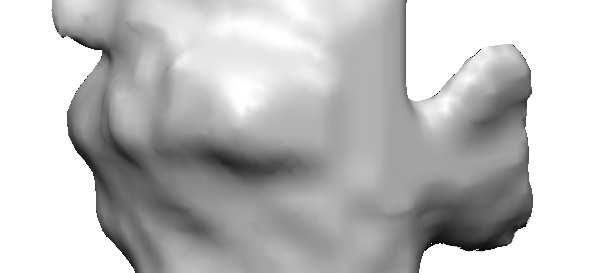
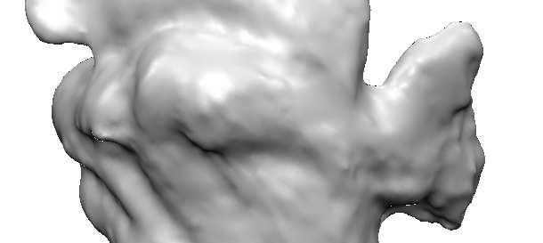
7 (a) (b) (c) (d) (e) (f) (g) (h) Figure 8. Van Gogh dataset. (a) 3 of the 25 input images (b) The camera distribution. (c) Initial surface from silhouette reconstruction. (d) The outermost layer (transparent) and innermost layer (opaque) of SDG. (e) Shape reconstructed by Edge Cut. (f) Shape reconstructed by Node Cut. (g) Shape reconstructed by SDG Cut. (h) Structured light scanned shape. (a) (b) (c) (d) (e) (f) Figure 9. Fish dataset. (a) 3 of the 25 input images. (b) The camera distribution (c) Initial shape from silhouette reconstruction. (d) Shape reconstructed by SDG Cut. (e) Structured light scanned shape. (f) Reconstructed surface by Edge Cut (left), Node Cut (middle) and by Soatto et al. [13] (right). Tail and fins are prone to be cut due to the minimal surface bias.

8 Table 1. Volume difference ratio V ol/v ol(s gt ) for Silhouette Intersection, Edge Cut, Node Cut, SDG Cut results and those reported by Jin et al.[7]. (1) Van Gogh dataset. (2) Fish dataset. Initial E-Cut N-Cut SDG Cut Jin et al.[7] 1 8.4% 9.1% 7.6% 4.0% 5.7% % 15.0% 14.5% 7.6% N/A measure, which must also be done in any other methods. To evaluate the reconstruction results quantitatively, we compute the volume difference between ground truth and the estimated surface. The difference V ol is defined as: V ol = V ol(s est Sgt ) V ol(s est Sgt ) (11) where S est is the estimated surface and S gt is the ground truth surface. The ratio V ol/v ol(s gt ) for different algorithms is listed in Table.1. Due to the biases, Edge Cut can sometimes perform even worse than the initialization 6. For Van Gogh dataset, our algorithm also improves on the result reported in [7]. Note that although visually the surface reconstructed by the level set method usually appears smoother, it still suffers from the minimal surface bias. Our algorithm works better in preserving the edges and corners, which results in a lower volume difference. 5 Conclusions and Future Work We discussed the two types of biases, the minimal surface bias and the discretization bias, associated with the current volumetric graph cut reconstruction algorithms. We proposed to reduce these biases by applying graph cut method on the SDG. SDG is constructed from the signed distance transform of an initial surface. It can be shown that for surfaces with no more than one intersection with each vertex trajectory of SDG, the optimal cut has no minimal surface bias. SDG also transforms the discretization bias into a controllable degree of surface smoothness. By applying the Graph Cuts on SDG we can obtain robust reconstruction under fluctuating photo-consistency measure of non-lambertian reflectance. Experimental results on two real datasets show the effectiveness of our algorithm. The current SDG Cut algorithm cannot handle topology change. However, the change is possible between two SDG Cut iterations, by using more flexible mesh to signed distance transform conversion. We plan to investigate further 6 Performance worse than the initial surface estimate is possible since these methods search for global minimum and are not affected by the initialization. The only constraint from the initialization is that the result should be within a pre-specified distance from the initial surface. on this. Also, our algorithm is not restricted to surface reconstruction. It can be applied to other reconstruction problems such as shape from shading and volumetric image segmentation. References [1] Y. Boykov and V. Kolmogorov. Computing geodesics and minimal surfaces via graph cuts. In Proceedings of ICCV 03, page 26, [2] Y. Boykov and V. Kolmogorov. An experimental comparison of min-cut/max- flow algorithms for energy minimization in vision. IEEE Trans. PAMI, 26(9): , [3] J. E. Davis, R. Yang, and L. Wang. Brdf invariant stereo using light transport constancy. In Proceedings of ICCV 05, volume 1, [4] O. Faugeras and R. Keriven. Variational principles, surface evolution, PDE s, level set methods and the stereo problem. IEEE Trans. Image Processing, 7(3): , [5] A. Georghiades. Incorporating the torrance and sparrow model of reflectance in uncalibrated photometric stereo. In Proc. CVPR 01, volume 2, pages , [6] A. Hertzmann and S. M. Seitz. Example-based photometric stereo: Shape reconstruction with general, varying brdfs. IEEE Trans. PAMI, 27(8): , [7] H. Jin, S. Soatto, and A. J. Yezzi. Multi-view stereo reconstruction of dense shape and complex appearance. Int. J. Comput. Vision, 63(3): , [8] V. Kolmogorov and R. Zabih. Multi-camera scene reconstruction via graph cuts. In Proceedings of ECCV 02 - Part III, pages 82 96, London, UK, Springer-Verlag. [9] K. N. Kutulakos and S. M. Seitz. A theory of shape by space carving. Int. J. Comput. Vision, 38(3): , [10] K. M. Lee and C.-C. J. Kuo. Shape from shading with a generalized reflectance map model. Comput. Vis. Image Underst., 67(2): , [11] D. Scharstein and R. Szeliski. A taxonomy and evaluation of dense two-frame stereo correspondence algorithms. Int. J. Comput. Vision, 47(1/2/3):7 42, [12] S. Seitz and C. Dyer. Photorealistic scene reconstruction by voxel coloring. Int. J. Comput. Vision, 35(2): , [13] S. Soatto, A. J. Yezzi, and H. Jin. Tales of shape and radiance in multi-view stereo. In Proceedings of ICCV 03, page 974, [14] G. Vogiatzis, P. H. S. Torr, and R. Cipolla. Multi-view stereo via volumetric graph-cuts. In Proceedings of CVPR 05, pages , Washington, DC, USA, [15] N. Xu, T. Yu, and N. Ahuja. Shape from color consistency using node cut. In Proceedings of Asian Conference on Computer Vision 2004, [16] R. Yang, M. Pollefeys, and G. Welch. Dealing with textureless regions and specular highlights-a progressive space carving scheme using a novel photo-consistency measure. In Proceedings of ICCV 03, page 576, [17] T. Zickler, P. N. Belhumeur, and D. J. Kriegman. Helmholtz stereopsis: Exploiting reciprocity for surface reconstruction. Int. J. Comput. Vision, 49(2-3): , 2002.