Imaging and Deconvolution
|
|
|
- Beverly Henderson
- 5 years ago
- Views:
Transcription


1 Imaging and Deconvolution Urvashi Rau National Radio Astronomy Observatory, Socorro, NM, USA


2 The van-cittert Zernike theorem Ei E V ij u, v = I l, m e sky j 2 i ul vm dldm 2D Fourier transform : Image = sum of cosine 'fringes'. Each antenna-pair measures the parameters of one 'fringe'. Amplitude, Phase : Ei E j is complex. Orientation, Wavelength : Geometry I sky l, m Sky Coordinates V u, v Spatial Frequencies
3 Measuring the visibility function Spatial Frequency : Length and orientation of the vector between two antennas, projected onto the plane perpendicular to the line of sight. u, v [ ] [ ][ ] u x v = R h, y w z w b z,h x, y j i x Ei E j, N antennas N(N-)/2 antenna-pairs (baselines) For each antenna pair, u, v change with time (hour-angle, declination) and observing frequency. Time and Frequency-resolution of the data samples, decides u, v Image is real => Visibility function is Hermitian : V u, v =V u, v => One baseline : 2 visibility points
4 Spatial Frequency (uv) coverage + Observed Image [ ] [ ][ ] u x v = R h, y w z S u, v Image of the sky using 2 antennas I obs l, m
5 Spatial Frequency (uv) coverage + Observed Image [ ] [ ][ ] u x v = R h, y w z S u, v Image of the sky using 5 antennas I obs l, m
6 Spatial Frequency (uv) coverage + Observed Image [ ] [ ][ ] u x v = R h, y w z S u, v Image of the sky using antennas I obs l, m
7 Spatial Frequency (uv) coverage + Observed Image [ ] [ ][ ] u x v = R h, y w z S u, v Image of the sky using 27 antennas I obs l, m
8 Spatial Frequency (uv) coverage + Observed Image [ ] [ ][ ] u x v = R h, y w z S u, v Image of the sky using 27 antennas over 2 hours 'Earth Rotation Synthesis' I obs l, m
9 Spatial Frequency (uv) coverage + Observed Image [ ] [ ][ ] u x v = R h, y w z S u, v Image of the sky using 27 antennas over 4 hours 'Earth Rotation Synthesis' I obs l, m
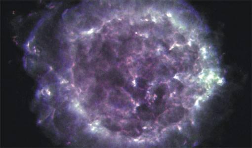
![Spatial Frequency (uv) coverage + Observed Image [ ] [ ][ ] u x v = R h, y w z S u, v Image](/docs-images/86/94949502/images/10-1.jpg "of the sky using 27 antennas over 4 hours, 2 frequencies 'Multi-Frequency Synthesis' I obs l,")
10 Spatial Frequency (uv) coverage + Observed Image [ ] [ ][ ] u x v = R h, y w z S u, v Image of the sky using 27 antennas over 4 hours, 2 frequencies 'Multi-Frequency Synthesis' I obs l, m
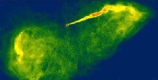
![Spatial Frequency (uv) coverage + Observed Image [ ] [ ][ ] u x v = R h, y w z S u, v Image](/docs-images/86/94949502/images/11-0.jpg "of the sky using 27 antennas over 4 hours, 3 frequencies 'Multi-Frequency Synthesis' I obs l,")
11 Spatial Frequency (uv) coverage + Observed Image [ ] [ ][ ] u x v = R h, y w z S u, v Image of the sky using 27 antennas over 4 hours, 3 frequencies 'Multi-Frequency Synthesis' I obs l, m
12 Point Spread Function ( PSF ) I psf l, m = F [S u, v ] S u, v The PSF is the inverse Fourier transform of the UV-coverage The PSF is --- the impulse-response of the instrument ( image of a point-source ) --- the intensity of the diffraction pattern through an array of 'slits' ( dishes ) --- a measure of the imaging-properties of the instrument angular resolution, ( max uv-spacing ) peak sensitivity, ( # measurements ) sidelobe levels, no total power ( missing spacings ) ( central uv-hole )
13 Image formed by an interferometer : Convolution Equation obs I l, m = I PSF sky l, m I l, m => You have measured the Convolution of the True Sky with the instrumental PSF. => Recovering the True Sky > DE-convolution First Step : Construct the PSF image, and the OBSERVED image...
14 Imaging in practice : Choosing image size, cell-size Choosing image 'cell' size : Nyquist-sample the main lobe of the PSF PSF beam width : 80 ( x to convert to degrees ) = radians bmax u max This is the diffraction-limited angular-resolution of the telescope Ex : Max baseline : 0 km. Freq = GHz. Angular resolution : 6 arcsec Choosing image field-of-view (npixels) : As much as desired/practical. = u fov rad Field of View (fov) controls the uv-grid-cell size u, v - Antenna primary-beam limits the field-of-view ( 'slits' of finite width ) Gridding + FFT : An interferometer measures irregularly spaced points on the UV-plane. Need to place the visibilities onto a regular grid of UV-pixels, and then take an FFT
15 Imaging in practice : Gridding and Weighting v An Image is a weighted-average of the data. v Natural Weights u u -- Visibility data are recorded onto a regular grid before taking an i-fft Convolutional Resampling => Use a gridding convolution function => Use weights per visibility (weighted average of all data points per cell) v Uniform Weights u
16 Imaging in practice : Weighting schemes An Image is a weighted average of the data. Choose a weighting-scheme => modify the imaging properties of the instrument => emphasize features/scales of interest => control imaging sensitivity Uniform/Robust Natural/Robust UV-Taper All spatialfrequencies get equal weight All data points get equal weight Low spatial freqs get higher weight than others higher medium lower PSF Sidelobes (VLA) lower higher depends Point Source Sensitivity lower maximum lower Extended Source Sensitivity lower medium higher Resolution

17 Imaging in practice : PSFs and Observed (dirty) Images Natural Robust 0.7 Uniform Bm : 5.6 arcsec 0. sidelobe Bm : 4.0 arcsec 0.05 sidelobe Bm : 3.2 arcsec +0.03,-0.08 sidelobe Tapered Uniform Bm : 8.0arcsec 0.0 sidelobe PSF OBSERVED Note the noise-structure. Noise is correlated between pixels by the PSF All pairs of images satisfy the convolution relation => Need to deconvolve them Image Units (Jy/beam)

 Major Cycle ( Imaging ) MODEL IMAGE")
18 Iterative Image Reconstruction Major and Minor Cycles DATA MODEL RESIDUAL RESIDUAL IMAGE GRIDDING ifft Use Flags and Weights Minor Cycle ( Deconvolution ) Major Cycle ( Imaging ) MODEL IMAGE FFT DE-GRIDDING
19 Deconvolution Hogbom CLEAN Sky Model : List of delta-functions () Construct the observed (dirty) image and PSF (2) Search for the location of peak amplitude. (3) Add a delta-function of this peak/location to the model (4) Subtract the contribution of this component from the dirty image - a scaled/shifted copy of the PSF Repeat steps (2), (3), (4) until a stopping criterion is reached. (5) Restore : Smooth the model with a 'clean beam' and add residuals The CLEAN algorithm can be formally derived as a model-fitting problem model parameters : locations and amplitudes of delta functions solution process : 2 minimization via an iterative steepest-descent algorithm ( method of successive approximation )
20 Deconvolution MS-CLEAN Multi-Scale Sky Model : Linear combination of 'blobs' of different scale sizes - Efficient representation of both compact and extended structure (sparse basis) A scale-sensitive algorithm () Choose a set of scale sizes (2) Calculate dirty/residual images smoothed to several scales (basis functions) Normalize by the relative sum-of-weights (instrument's sensitivity to each scale) (3) Find the peak across all scales, update a single multi-scale model as well as all residual images (using information about coupling between scales) Iterate, similar to Classic CLEAN, and restore at the end. The MS-CLEAN algorithm can also be formally derived as a model-fitting problem using 2 minimization and a basis set consisting of several 'blob' sizes.

21 Deconvolution Comparison of Algorithms CLEAN Minimize L2 (assume sparsity in the image) MEM Minimize L2 subject to an entropy-based prior (e.g. smoothness) MS-CLEAN Minimize L2 (assume a set of spatial scales) ASP Minimize L2 with TV-based subspace searches Im I out
")

 ASP Minimize L2 with")
22 Deconvolution Comparison of Algorithms CLEAN Minimize L2 (assume sparsity in the image) MEM Minimize L2 subject to an entropy-based prior (e.g. smoothness) MS-CLEAN Minimize L2 (assume a set of spatial scales) ASP Minimize L2 with TV-based subspace searches Im I res

23 Image Quality Noise in the image : Measured from restored or residual images With perfect reconstruction, The ideal noise level is : RMS Model image T sys 0.2 a N ant N ant N pol In reality, measure the RMS of residual pixel amplitudes Dynamic Range : Measured from the restored image Restored image Standard : Ratio of peak brightness to RMS noise in a region devoid of emission. More truthful : Ratio of peak brightness to peak error (residual) Residual image Image Fidelity : Correctness of the reconstruction - remember the infinite possibilities that fit the data perfectly? - useful only if a comparison image exists. m beam I I Inverse of relative error : I m I beam I restored
24 How can you control the quality of image reconstruction? () Iterations and stopping criterion 'niter' : maximum number of iterations / components 'threshold' : don't search for flux below this level minor cycles can be inaccurate, so periodically trigger major cycles (2) Using masks Need masks only if the deconvolution is hard. => Bad PSFs with high sidelobes => Leftover bad data causing stripes or ripples => Extended emission with sharp edges => Extended emission that is seen only by very few baselines Can draw them interactively (start small, and grow them) or supply final mask. (3) Self-Calibration Use your current best estimate of the sky ( i.e. the model image ) to get new antenna gain solutions. Apply them. Image again and repeat.


25 Wide-band Imaging Sensitivity and Multi-Frequency Synthesis Frequency Range : ( 2 GHz) (4 8 GHz) (8 2 GHz) GHz 4 GHz 4 GHz Bandwidth Ratio : max : min 2: 2:.5 : Fractional Bandwidth : max min / mid 66% 66% 40% Bandwidth : max min UV-coverage / imaging properties change with frequency.0 GHz.5 GHz 2.0 GHz GHz b b S u, v = = c => combine multi-frequency measurements during imaging Sky Brightness can also change with frequency model intensity and spectrum
26 Spectral Cube (vs) MFS imaging Simulation : 3 flat-spectrum sources + steep-spectrum source ( -2 GHz VLA observation ) Images made at different frequencies between and 2 GHz ( limited to narrow-band sensitivity ) GHz Add all singlefrequency images (after smoothing to a low resolution) 2 GHz Use wideband UVcoverage, but ignore spectrum ( MFS, nterms=) Use wideband UV-coverage + Model and fit for spectra too ( MT-MFS, nterms > ) Output : Intensity and Spectral-Index
27 Wide-Field Imaging W-term V obs u, v =S u, v I l, m e2 i ul vm dl dm V obs u, v =S u, v I l, m e 2 i ul vm w n dl dm dn The ' w ' component of a baseline can be large, away from the image phase center The ' n ' component of a source can be large, away from the image phase center w w There are algorithms to account for this : Image Faceting, W-Projection. n
28 Wide-Field Imaging Primary Beams Each antenna has a limited field of view => Primary Beam (gain) pattern => Sky is (approx) multiplied by PB, before being sampled by the interferometer I obs (l, m) I PSF (l, m) [ P (l, m) I sky sky (l, m) ] The antenna field of view : D = antenna diameter λ/ D D bmax Compare with angular resolution of the interferometer : λ/b max Output Image = Sky x PB But, in reality, P changes with time, freq, pol and antenna... => Ignoring such effects limits dynamic range to 0^4 => More-accurate method to account for this : A-Projection
 pattern => Sky is (approx) multiplied by")
 [ P (l, m) I sky sky (l, m) ] The antenna field of view : D =")


29 Wide-Field Imaging Primary Beams Each antenna has a limited field of view => Primary Beam (gain) pattern => Sky is (approx) multiplied by PB, before being sampled by the interferometer I obs (l, m) I PSF (l, m) [ P (l, m) I sky sky (l, m) ] The antenna field of view : D = antenna diameter λ/ D D bmax Compare with angular resolution of the interferometer : λ/b max PB-corrected Image : Sky But, in reality, P changes with time, freq, pol and antenna... => Ignoring such effects limits dynamic range to 0^4 => More-accurate method to account for this : A-Projection
 Grid all data")
30 Wide-field Imaging -- Mosaics Combine data from multiple pointings to form one large image. Combine pointings either before or after deconvolution. Stitched mosaic : -- Deconvolve each pointing separately -- Divide each image by PB -- Combine as a weighted avg Joint mosaic : -- Combine observed images as a weighted average (or) Grid all data onto one UV-grid, and then ifft -- Deconvolve as one large image One Pointing sees only part of the source
 Grid all data")
31 Wide-field Imaging -- Mosaics Combine data from multiple pointings to form one large image. Combine pointings either before or after deconvolution. Stitched mosaic : -- Deconvolve each pointing separately -- Divide each image by PB -- Combine as a weighted avg Joint mosaic : -- Combine observed images as a weighted average (or) Grid all data onto one UV-grid, and then ifft -- Deconvolve as one large image Two Pointings see more...
32 Wide-field Imaging -- Mosaics Combine data from multiple pointings to form one large image. Combine pointings either before or after deconvolution. Stitched mosaic : -- Deconvolve each pointing separately -- Divide each image by PB -- Combine as a weighted avg Joint mosaic : -- Combine observed images as a weighted average (or) Grid all data onto one UV-grid, and then ifft Use many pointings to cover the source with approximately uniform sensitivity -- Deconvolve as one large image
33 Some points to remember How does an interferometer form an image? - Each antenna pair measures one 2D fringe. Many antenna pairs => Fourier series How do you make a raw image from interferometer data? - Assign weights to visibilities, grid them, take a Fourier transform How do you choose the cell-size and image size for imaging? - Cell size = ( angular resolution / 3 ). Image size = field-of-view / cell size What does the raw observed image represent? - Observed Sky is the convolution of the true sky and the PSF How do you get a model of the sky? - Solve the convolution equation via algorithms like Clean, MS-Clean, MT-Clean...
34 Some points to remember How do you measure image quality? - RMS noise, Peak residual, Dynamic range, Image fidelity How does wide-band data affect the imaging process? - Increased sensitivity, but the imaging properties and sky change with frequency How do you image wide-band data? - Make a Cube of images, or Multi-Frequency-Synthesis with a spectral fit. What is an antenna primary beam and what is its effect on an image? - Antenna power pattern. It multiplies with the sky, before convolution with the PSF What is the w-term problem? - 2D Fourier transform approximations are invalid far away from the image center
35 Example Imaging Problem Simulated data Simulated 5 GHz observation with a 3-antenna array over 5 hours N visibilities : Visibility noise : 2 Jy => Theoretical image RMS : 0.02 Jy Angular resolution : 5 arcsec ( Max baseline of 2500m at 5.0 GHz ) Sky brightness has compact and extended structure (partially-sampled). Peak brightness : Jy => Target dynamic range = 50 I sky l, m S u, v V sky u, v S u, v
36 Example Imaging Problem First try... Quick deconvolution with different weighting schemes : Image FOV : 7 arcmin ( 52 pixels at 0.8 arcsec pixel size ) MS-CLEAN : NIter=00, scales=[0,6,40], gain=0.3, robust=0.7 Natural High sidelobes Uniform with a uvtaper for 9 arcsec Robust = 0.7 Uniform with only SHORT Baselines < 500m Uniform Low sensitivity to extended emission Uniform with only LONG Baselines > 500m ( Extended structure disappears )
37 Example Imaging Problem Second try... Make a larger image ( 700 pixels at 0.8 arcsec cell size ) N Iter = 0 (dirty image ) Pick scales = [0,6,6,30,42,60] Weighting : Robust=0.7 Loop gain = 0.2 ( go slow, because of insufficient dataconstraints for the extended emission ) Peak sidelobe structure : 0.2 Jy/beam. Off-source RMS : 0. Jy/beam Peak brightness : Jy/beam => Dynamic Range : 0 ~ 20
38 Example Imaging Problem Second try... After 00 iterations. Restored Image Residual Image Peak sidelobe structure : 0. Jy/beam. Off-source RMS : 0.05 Jy/beam Peak brightness : Jy/beam => Dynamic Range : 0 ~ 20
39 Example Imaging Problem Second try... After 500 iterations. Almost OK. Spurious extended flux in the upper-left. No counterpart in the residual image => large scales unconstrained by the data Restored Image Peak artifacts : 0.07 Jy/beam. Peak brightness : Jy/beam Residual Image Off-source RMS : 0.02 Jy/beam => Dynamic Range : 4 ~ 50 Reached theoretical off-source RMS of 0.02 Jy/beam. But peak residual is still high.
40 Example Imaging Problem Using masks Build 'CLEAN boxes' or masks and restart. This will force extended emission to be centered within the allowed regions only. In general, point sources do not require boxes. Extended emission needs it only if data constraints are insufficient.
41 Example Imaging Problem Third try... After 300 iterations ( compared to 500 earlier ) Reached theoretical rms and dynamic-range! ( in practice, this is not so easy... ) Restored Image Residual Image Peak sidelobe structure : 0.04 Jy/beam. Off-source RMS : 0.02 Jy/beam Peak brightness : Jy/beam => Dynamic Range : 25 ~ 50
Imaging and Deconvolution
 Imaging and Deconvolution 24-28 Sept 202 Narrabri, NSW, Australia Outline : - Synthesis Imaging Concepts - Imaging in Practice Urvashi Rau - Image-Reconstruction Algorithms National Radio Astronomy Observatory
Synthesis Imaging. Claire Chandler, Sanjay Bhatnagar NRAO/Socorro
 Synthesis Imaging Claire Chandler, Sanjay Bhatnagar NRAO/Socorro Michelson Summer Workshop Caltech, July 24-28, 2006 Synthesis Imaging 2 Based on the van Cittert-Zernike theorem: The complex visibility
Sky-domain algorithms to reconstruct spatial, spectral and time-variable structure of the sky-brightness distribution
 Sky-domain algorithms to reconstruct spatial, spectral and time-variable structure of the sky-brightness distribution Urvashi Rau National Radio Astronomy Observatory Socorro, NM, USA Outline : - Overview
How accurately do our imaging algorithms reconstruct intensities and spectral indices of weak sources?
 How accurately do our imaging algorithms reconstruct intensities and spectral indices of weak sources? Urvashi Rau, Sanjay Bhatnagar, Frazer Owen ( NRAO ) 29th Annual New Mexico Symposium, NRAO, Socorro,
Imaging and non-imaging analysis
 1 Imaging and non-imaging analysis Greg Taylor University of New Mexico Spring 2017 Plan for the lecture-i 2 How do we go from the measurement of the coherence function (the Visibilities) to the images
Basic Imaging and Self- Calibration (T4 + T7)
") Basic Imaging and Self- Calibration (T4 + T7) John McKean Visibilities Fourier Transform Deconvolution AIM: 1. To make an image by taking the fast Fourier transform of the visibility data. 2. Carry out
Basic Imaging and Self- Calibration (T4 + T7) John McKean Visibilities Fourier Transform Deconvolution AIM: 1. To make an image by taking the fast Fourier transform of the visibility data. 2. Carry out
Lecture 17 Reprise: dirty beam, dirty image. Sensitivity Wide-band imaging Weighting
 Lecture 17 Reprise: dirty beam, dirty image. Sensitivity Wide-band imaging Weighting Uniform vs Natural Tapering De Villiers weighting Briggs-like schemes Reprise: dirty beam, dirty image. Fourier inversion
ADVANCED RADIO INTERFEROMETRIC IMAGING
 ADVANCED RADIO INTERFEROMETRIC IMAGING Hayden Rampadarath Based upon J. Radcliffe's DARA presentation Image courtesy of NRAO/AUI INTR ODU CT ION In the first imaging lecture, we discussed the overall and
Imaging and Deconvolution
 Imaging and Deconvolution Rick Perley, NRAO/Socorro ATNF Radio School Narrabri, NSW 29 Sept 03 Oct 2014 #G Topics Imaging Formal Solution Discrete Data The Direct Transform The Fast Fourier Transform Weighting,
The Techniques of Radio Interferometry III: Imaging
 Master Astronomy and Astrophysics - 5214RAAS6Y Radio Astronomy Lecture 8 The Techniques of Radio Interferometry III: Imaging Lecturer: Michael Wise (wise@astron.nl) April 25th, 2013 Westerbork/LOFAR Field
Imaging and Deconvolution
 Imaging and Deconvolution David J. Wilner (Harvard-Smithsonian Center for Astrophysics) Fifteenth Synthesis Imaging Workshop 1-8 June 2016 Overview gain some intuition about interferometric imaging understand
ALMA Memo 386 ALMA+ACA Simulation Tool J. Pety, F. Gueth, S. Guilloteau IRAM, Institut de Radio Astronomie Millimétrique 300 rue de la Piscine, F-3840
 ALMA Memo 386 ALMA+ACA Simulation Tool J. Pety, F. Gueth, S. Guilloteau IRAM, Institut de Radio Astronomie Millimétrique 300 rue de la Piscine, F-38406 Saint Martin d'h eres August 13, 2001 Abstract This
ERROR RECOGNITION and IMAGE ANALYSIS
 PREAMBLE TO ERROR RECOGNITION and IMAGE ANALYSIS 2 Why are these two topics in the same lecture? ERROR RECOGNITION and IMAGE ANALYSIS Ed Fomalont Error recognition is used to determine defects in the data
Radio Interferometry Bill Cotton, NRAO. Basic radio interferometry Emphasis on VLBI Imaging application
 Radio Interferometry Bill Cotton, NRAO Basic radio interferometry Emphasis on VLBI Imaging application 2 Simplest Radio Interferometer Monochromatic, point source 3 Interferometer response Adding quarter
Wideband Mosaic Imaging for VLASS
 Wideband Mosaic Imaging for VLASS Preliminary ARDG Test Report U.Rau & S.Bhatnagar 29 Aug 2018 (1) Code Validation and Usage (2) Noise, Weights, Continuum sensitivity (3) Imaging parameters (4) Understanding
High dynamic range imaging, computing & I/O load
 High dynamic range imaging, computing & I/O load RMS ~15µJy/beam RMS ~1µJy/beam S. Bhatnagar NRAO, Socorro Parameterized Measurement Equation Generalized Measurement Equation Obs [ S M V ij = J ij, t W
CASA. Algorithms R&D. S. Bhatnagar. NRAO, Socorro
 Algorithms R&D S. Bhatnagar NRAO, Socorro Outline Broad areas of work 1. Processing for wide-field wide-band imaging Full-beam, Mosaic, wide-band, full-polarization Wide-band continuum and spectral-line
Radio interferometric imaging of spatial structure that varies with time and frequency
 Radio interferometric imaging of spatial structure that varies with time and frequency Urvashi Rau National Radio Astronomy Observatory, 1003 Lopezville Road, Socorro, NM-87801, USA ABSTRACT The spatial-frequency
Synthesis imaging using CASA
 Synthesis imaging using CASA Kuo-Song Wang ( 國松) and ARC-Taiwan team (ASIAA) UCAT Summer Student Program 2016 2016/06/30 Recap Radio interferometric observations The products from the array are Visibilities
High Dynamic Range Imaging
 High Dynamic Range Imaging Josh Marvil CASS Radio Astronomy School 3 October 2014 CSIRO ASTRONOMY & SPACE SCIENCE High Dynamic Range Imaging Introduction Review of Clean Self- Calibration Direction Dependence
Lessons learnt from implementing mosaicing and faceting in ASKAPsoft. Max Voronkov & Tim Cornwell ASKAP team 2nd April 2009
 Lessons learnt from implementing mosaicing and faceting in ASKAPsoft Max Voronkov & Tim Cornwell ASKAP team 2nd April 2009 Outline - Imaging software ASKAPsoft re-uses LOFAR design Imaging is treated as
Continuum error recognition and error analysis
 Continuum error recognition and error analysis Robert Laing (ESO) 1 Outline Error recognition: how do you recognise and diagnose residual errors by looking at images? Image analysis: how do you extract
Fast Holographic Deconvolution
 Precision image-domain deconvolution for radio astronomy Ian Sullivan University of Washington 4/19/2013 Precision imaging Modern imaging algorithms grid visibility data using sophisticated beam models
Deconvolution and Imaging ASTR 240: In-class activity, April 1, 2013
 Deconvolution and Imaging ASTR 240: In-class activity, April 1, 2013 In this activity, we will use calibrated visibilities from the Submillimeter Array to create an image of a disk around a nearby young
Image Pixelization and Dynamic Range
 EVLA Memo 114 Image Pixelization and Dynamic Range W. D. Cotton, Juan M. Uson NRAO 1 Abstract This study investigates some of the effects of representing the sky by a rectangular grid of pixels on the
Wide-field Wide-band Full-Mueller Imaging
 Wide-field Wide-band Full-Mueller Imaging CALIM2016, Oct. 10th 2016, Socorro, NM S. Bhatnagar NRAO, Socorro The Scientific Motivation Most projects with current telescopes require precise reconstruction
Wide-Field Imaging I: Non-Coplanar Visibilities
 Wide-Field Imaging I: Non-Coplanar Visibilities Rick Perley Eleventh Synthesis Imaging Workshop Socorro, June 10-17, 2008 Review: Measurement Equation From the first lecture, we have a general relation
OSKAR-2: Simulating data from the SKA
 OSKAR-2: Simulating data from the SKA AACal 2012, Amsterdam, 13 th July 2012 Fred Dulwich, Ben Mort, Stef Salvini 1 Overview OSKAR-2: Interferometer and beamforming simulator package. Intended for simulations
EVLA Memo #132 Report on the findings of the CASA Terabyte Initiative: Single-node tests
 EVLA Memo #132 Report on the findings of the CASA Terabyte Initiative: Single-node tests S. Bhatnagar NRAO, Socorro May 18, 2009 Abstract This note reports on the findings of the Terabyte-Initiative of
Spectrographs. C. A. Griffith, Class Notes, PTYS 521, 2016 Not for distribution.
 Spectrographs C A Griffith, Class Notes, PTYS 521, 2016 Not for distribution 1 Spectrographs and their characteristics A spectrograph is an instrument that disperses light into a frequency spectrum, which
A Modified Algorithm for CLEANing Wide-Field Maps with Extended Structures
 J. Astrophys. Astr. (1990) 11, 311 322 A Modified Algorithm for CLEANing Wide-Field Maps with Extended Structures Κ. S. Dwarakanath, A. A. Deshpande & Ν. Udaya Shankar Raman Research institute, Bangalore
IRAM Memo MAPPING for NOEMA: Concepts and Usage
 Original version at http://iram-institute.org/medias/uploads/mapping-noema.pdf IRAM Memo 2016-1 MAPPING for NOEMA: Concepts and Usage S. Guilloteau 1 1. LAB (Bordeaux) 14-Jul-2016 version 1.0 09-Sep-2016
OSKAR: Simulating data from the SKA
 OSKAR: Simulating data from the SKA Oxford e-research Centre, 4 June 2014 Fred Dulwich, Ben Mort, Stef Salvini 1 Overview Simulating interferometer data for SKA: Radio interferometry basics. Measurement
GBT Memo #300: Correcting ALMA 12-m Array Data for Missing Short Spacings Using the Green Bank Telescope
 GBT Memo #300: Correcting ALMA 12-m Array Data for Missing Short Spacings Using the Green Bank Telescope Melissa Hoffman and Amanda Kepley 28 September 2018 Contents 1 Introduction 1 2 Data 2 2.1 Observations
Correlator Field-of-View Shaping
 Correlator Field-of-View Shaping Colin Lonsdale Shep Doeleman Vincent Fish Divya Oberoi Lynn Matthews Roger Cappallo Dillon Foight MIT Haystack Observatory Context SKA specifications extremely challenging
ERROR RECOGNITION & IMAGE ANALYSIS. Gustaaf van Moorsel (NRAO) Ed Fomalont (NRAO) Twelfth Synthesis Imaging Workshop 2010 June 8-15
 Ed Fomalont (NRAO) Twelfth Synthesis Imaging Workshop 2010 June 8-15") ERROR RECOGNITION & IMAGE ANALYSIS Gustaaf van Moorsel (NRAO) Ed Fomalont (NRAO) Twelfth Synthesis Imaging Workshop 2010 June 8-15 INTRODUCTION Why are these two topics Error Recognition and Image Analysis
ERROR RECOGNITION & IMAGE ANALYSIS Gustaaf van Moorsel (NRAO) Ed Fomalont (NRAO) Twelfth Synthesis Imaging Workshop 2010 June 8-15 INTRODUCTION Why are these two topics Error Recognition and Image Analysis
( ) = First Bessel function, x = π Dθ
 = First Bessel function, x = π Dθ") Observational Astronomy Image formation Complex Pupil Function (CPF): (3.3.1) CPF = P( r,ϕ )e ( ) ikw r,ϕ P( r,ϕ ) = Transmittance of the aperture (unobscured P = 1, obscured P = 0 ) k = π λ = Wave number
Observational Astronomy Image formation Complex Pupil Function (CPF): (3.3.1) CPF = P( r,ϕ )e ( ) ikw r,ϕ P( r,ϕ ) = Transmittance of the aperture (unobscured P = 1, obscured P = 0 ) k = π λ = Wave number
Michelson Interferometer
 Michelson Interferometer The Michelson interferometer uses the interference of two reflected waves The third, beamsplitting, mirror is partially reflecting ( half silvered, except it s a thin Aluminum
ALMA simulations Rosita Paladino. & the Italian ARC
 ALMA simulations Rosita Paladino & the Italian ARC Two software tools available to help users simulate images resulting from an ALMA observations: Simulations with CASA tasks sim_observe & sim_analyze
Data Analysis. I have got some data, so what now? Naomi McClure-Griffiths CSIRO Australia Telescope National Facility 2 Oct 2008
 Data Analysis I have got some data, so what now? Naomi McClure-Griffiths CSIRO Australia Telescope National Facility 2 Oct 2008 1 Outline Non-imaging analysis Parameter estimation Point source fluxes,
EVLA memo 77. EVLA and SKA computing costs for wide field imaging. (Revised) 1. T.J. Cornwell, NRAO 2
 1. T.J. Cornwell, NRAO 2") EVLA memo 77 EVLA and SKA computing costs for wide field imaging (Revised) 1 T.J. Cornwell, NRAO 2 tcornwel@nrao.edu Abstract: I investigate the problem of high dynamic range continuum imaging in the presence
EVLA memo 77 EVLA and SKA computing costs for wide field imaging (Revised) 1 T.J. Cornwell, NRAO 2 tcornwel@nrao.edu Abstract: I investigate the problem of high dynamic range continuum imaging in the presence
Antenna Configurations for the MMA
 MMA Project Book, Chapter 15: Array Configuration Antenna Configurations for the MMA Tamara T. Helfer & M.A. Holdaway Last changed 11/11/98 Revision History: 11/11/98: Added summary and milestone tables.
van Cittert-Zernike Theorem
 van Cittert-Zernike Theorem Fundamentals of Radio Interferometry, Section 4.5 Griffin Foster SKA SA/Rhodes University NASSP 2016 What is the Fourier transform of the sky? NASSP 2016 2:21 Important Points:
Visualization & the CASA Viewer
 Visualization & the Viewer Juergen Ott & the team Atacama Large Millimeter/submillimeter Array Expanded Very Large Array Robert C. Byrd Green Bank Telescope Very Long Baseline Array Visualization Goals:
Image Processing and Analysis
 Image Processing and Analysis 3 stages: Image Restoration - correcting errors and distortion. Warping and correcting systematic distortion related to viewing geometry Correcting "drop outs", striping and
Imaging Supermassive Black Holes with the Event Horizon Telescope
 Counter Jet Model Forward Jet Kazunori Akiyama, NEROC Symposium: Radio Science and Related Topics, MIT Haystack Observatory, 11/04/2016 Imaging Supermassive Black Holes with the Event Horizon Telescope
ASKAP Pipeline processing and simulations. Dr Matthew Whiting ASKAP Computing, CSIRO May 5th, 2010
 ASKAP Pipeline processing and simulations Dr Matthew Whiting ASKAP Computing, CSIRO May 5th, 2010 ASKAP Computing Team Members Team members Marsfield: Tim Cornwell, Ben Humphreys, Juan Carlos Guzman, Malte
Adaptive selfcalibration for Allen Telescope Array imaging
 Adaptive selfcalibration for Allen Telescope Array imaging Garrett Keating, William C. Barott & Melvyn Wright Radio Astronomy laboratory, University of California, Berkeley, CA, 94720 ABSTRACT Planned
Imaging and Image Analysis
 Imaging and Image Analysis Urvashi R.V. National Radio Astronomy Observatory, Socorro, NM, USA 6th VLA Data Reduction Workshop ( 23 27 October, 2017 ) Outline - Synthesis imaging as implemented in CASA
IRAM mm-interferometry School UV Plane Analysis. IRAM Grenoble
 IRAM mm-interferometry School 2004 1 UV Plane Analysis Frédéric Gueth IRAM Grenoble UV Plane analysis 2 UV Plane analysis The data are now calibrated as best as we can Caution: data are calibrated, but
NRAO VLA Archive Survey
 NRAO VLA Archive Survey Jared H. Crossley, Loránt O. Sjouwerman, Edward B. Fomalont, and Nicole M. Radziwill National Radio Astronomy Observatory, 520 Edgemont Road, Charlottesville, Virginia, USA ABSTRACT
Controlling Field-of-View of Radio Arrays using Weighting Functions
 Controlling Field-of-View of Radio Arrays using Weighting Functions MIT Haystack FOV Group: Lynn D. Matthews,Colin Lonsdale, Roger Cappallo, Sheperd Doeleman, Divya Oberoi, Vincent Fish Fulfilling scientific
Theoretically Perfect Sensor
 Sampling 1/60 Sampling The ray tracer samples the geometry, only gathering information from the parts of the world that interact with a finite number of rays In contrast, a scanline renderer can push all
esac PACS Spectrometer: forward model tool for science use
 esac European Space Astronomy Centre (ESAC) P.O. Box, 78 28691 Villanueva de la Cañada, Madrid Spain PACS Spectrometer: forward model tool for science use Prepared by Elena Puga Reference HERSCHEL-HSC-TN-2131
RADIO ASTRONOMICAL IMAGE FORMATION USING SPARSE RECONSTRUCTION TECHNIQUES
 RADIO ASTRONOMICAL IMAGE FORMATION USING SPARSE RECONSTRUCTION TECHNIQUES Runny Levanda 1 1 School of Engineering Bar-Ilan University, Ramat-Gan, 5900, Israel Amir Leshem 1, Faculty of EEMCS Delft University
College Physics 150. Chapter 25 Interference and Diffraction
 College Physics 50 Chapter 5 Interference and Diffraction Constructive and Destructive Interference The Michelson Interferometer Thin Films Young s Double Slit Experiment Gratings Diffraction Resolution
Imaging Strategies and Postprocessing Computing Costs for Large-N SKA Designs
 Imaging Strategies and Postprocessing Computing Costs for Large-N SKA Designs Colin J. Lonsdale Sheperd S Doeleman Divya Oberoi MIT Haystack Observatory 17 July 2004 Abstract: The performance goals of
Theoretically Perfect Sensor
 Sampling 1/67 Sampling The ray tracer samples the geometry, only gathering information from the parts of the world that interact with a finite number of rays In contrast, a scanline renderer can push all
Computational issues for HI
 Computational issues for HI Tim Cornwell, Square Kilometre Array How SKA processes data Science Data Processing system is part of the telescope Only one system per telescope Data flow so large that dedicated
Chapter 9. Coherence
 Chapter 9. Coherence Last Lecture Michelson Interferometer Variations of the Michelson Interferometer Fabry-Perot interferometer This Lecture Fourier analysis Temporal coherence and line width Partial
Mosaicing and Single-Dish Combination
 Mosaicing and Single-Dish Combination CASS Radio Astronomy School 2012 Lister Staveley-Smith (ICRAR / CAASTRO / UWA) Outline Mosaicing with interferometers! Nyquist sampling! Image formation Combining
Advanced phase retrieval: maximum likelihood technique with sparse regularization of phase and amplitude
 Advanced phase retrieval: maximum likelihood technique with sparse regularization of phase and amplitude A. Migukin *, V. atkovnik and J. Astola Department of Signal Processing, Tampere University of Technology,
COMMENTS ON ARRAY CONFIGURATIONS. M.C.H. Wright. Radio Astronomy laboratory, University of California, Berkeley, CA, ABSTRACT
 Bima memo 66 - May 1998 COMMENTS ON ARRAY CONFIGURATIONS M.C.H. Wright Radio Astronomy laboratory, University of California, Berkeley, CA, 94720 ABSTRACT This memo briey compares radial, circular and irregular
Array Design. Introduction
 Introduction 2 Array Design Mark Wieringa (ATNF) Normally we use arrays the way they are.. Just decide on observing parameters and best configuration for particular experiment Now turn it around try to
To see how a sharp edge or an aperture affect light. To analyze single-slit diffraction and calculate the intensity of the light
 Diffraction Goals for lecture To see how a sharp edge or an aperture affect light To analyze single-slit diffraction and calculate the intensity of the light To investigate the effect on light of many
Self-calibration: about the implementation in GILDAS. Vincent Piétu IRAM. IRAM millimeter interferometry summerschool
 Self-calibration: about the implementation in GILDAS Vincent Piétu IRAM 1 About an interferometer sensitivity One usually considers only the noise equation to assess the feasibility of an observation.
SSW, Radio, X-ray, and data analysis
 SSW, Radio, X-ray, and data analysis Eduard Kontar School of Physics and Astronomy University of Glasgow, UK CESRA Summer School, Glasgow, August 2015 SSW Pre-school installation guide for IDL, SSW and
OSKAR Settings Files Revision: 8
 OSKAR Settings Files Version history: Revision Date Modification 1 212-4-23 Creation. 2 212-5-8 Added default value column to settings tables. 3 212-6-13 Updated settings for version 2..2-beta. 4 212-7-27
Chapter 5 Example and Supplementary Problems
 Chapter 5 Example and Supplementary Problems Single-Slit Diffraction: 1) A beam of monochromatic light (550 nm) is incident on a single slit. On a screen 3.0 meters away the distance from the central and
ALMA Antenna responses in CASA imaging
 ALMA Antenna responses in CASA imaging Dirk Petry (ESO), December 2012 Outline Motivation ALBiUS/ESO work on CASA responses infrastructure and ALMA beam library First test results 1 Motivation ALMA covers
Advanced Radio Imaging Techniques
 Advanced Radio Imaging Techniques Dylan Nelson August 10, 2006 MIT Haystack Observatory Mentors: Colin Lonsdale, Roger Cappallo, Shep Doeleman, Divya Oberoi Overview Background to the problem Data volumes
Computer Vision. Fourier Transform. 20 January Copyright by NHL Hogeschool and Van de Loosdrecht Machine Vision BV All rights reserved
 Van de Loosdrecht Machine Vision Computer Vision Fourier Transform 20 January 2017 Copyright 2001 2017 by NHL Hogeschool and Van de Loosdrecht Machine Vision BV All rights reserved j.van.de.loosdrecht@nhl.nl,
Modeling Antenna Beams
 Modeling Antenna Beams Walter Brisken National Radio Astronomy Observatory 2011 Sept 22 1 / 24 What to learn from this talk EM simulations of antennas can be complicated Many people have spent careers
Development of Focal-Plane Arrays and Beamforming Networks at DRAO
 Development of Focal-Plane Arrays and Beamforming Networks at DRAO Bruce Veidt Dominion Radio Astrophysical Observatory Herzberg Institute of Astrophysics National Research Council of Canada Penticton,
MAPPING. March 29th, Version 2.0. Questions? Comments? Bug reports? Mail to:
 i MAPPING A gildas software March 29th, 2007 Version 2.0 Questions? Comments? Bug reports? Mail to: gildas@iram.fr The gildas team welcomes an acknowledgment in publications using gildas software to reduce
Empirical Parameterization of the Antenna Aperture Illumination Pattern
 Empirical Parameterization of the Antenna Aperture Illumination Pattern Preshanth Jagannathan UCT/NRAO Collaborators : Sanjay Bhatnagar, Walter Brisken Measurement Equation The measurement equation in
Testbed experiment for SPIDER: A photonic integrated circuit-based interferometric imaging system
 Testbed experiment for SPIDER: A photonic integrated circuit-based interferometric imaging system Katherine Badham, Alan Duncan, Richard L. Kendrick, Danielle Wuchenich, Chad Ogden, Guy Chriqui Lockheed
From multiple images to catalogs
 Lecture 14 From multiple images to catalogs Image reconstruction Optimal co-addition Sampling-reconstruction-resampling Resolving faint galaxies Automated object detection Photometric catalogs Deep CCD
Primary Beams & Radio Interferometric Imaging Performance. O. Smirnov (Rhodes University & SKA South Africa)
") Primary Beams & Radio Interferometric Imaging Performance O. Smirnov (Rhodes University & SKA South Africa) Introduction SKA Dish CoDR (2011), as summarized by Tony Willis: My sidelobes are better than
Primary Beams & Radio Interferometric Imaging Performance O. Smirnov (Rhodes University & SKA South Africa) Introduction SKA Dish CoDR (2011), as summarized by Tony Willis: My sidelobes are better than
G Practical Magnetic Resonance Imaging II Sackler Institute of Biomedical Sciences New York University School of Medicine. Compressed Sensing
 G16.4428 Practical Magnetic Resonance Imaging II Sackler Institute of Biomedical Sciences New York University School of Medicine Compressed Sensing Ricardo Otazo, PhD ricardo.otazo@nyumc.org Compressed
Lecture 8 Object Descriptors
 Lecture 8 Object Descriptors Azadeh Fakhrzadeh Centre for Image Analysis Swedish University of Agricultural Sciences Uppsala University 2 Reading instructions Chapter 11.1 11.4 in G-W Azadeh Fakhrzadeh
PACS Spectrometer Simulation and the Extended to Point Correction
 PACS Spectrometer Simulation and the Extended to Point Correction Jeroen de Jong February 11, 2016 Abstract This technical note describes simulating a PACS observation with a model source and its application
Control of Light. Emmett Ientilucci Digital Imaging and Remote Sensing Laboratory Chester F. Carlson Center for Imaging Science 8 May 2007
 Control of Light Emmett Ientilucci Digital Imaging and Remote Sensing Laboratory Chester F. Carlson Center for Imaging Science 8 May 007 Spectro-radiometry Spectral Considerations Chromatic dispersion
Note 158: The AIPS++ GridTool Class How to use the GridTool class - definitions and tutorial
 Note 158: The AIPS++ GridTool Class How to use the GridTool class - definitions and tutorial Anthony G. Willis Copyright 1993 AIPS++ Chapter 2: Convolution in the Fourier Domain 1 Introduction The AIPS++
Chapter 82 Example and Supplementary Problems
 Chapter 82 Example and Supplementary Problems Nature of Polarized Light: 1) A partially polarized beam is composed of 2.5W/m 2 of polarized and 4.0W/m 2 of unpolarized light. Determine the degree of polarization
An imaging technique for subsurface faults using Teleseismic-Wave Records II Improvement in the detectability of subsurface faults
 Earth Planets Space, 52, 3 11, 2000 An imaging technique for subsurface faults using Teleseismic-Wave Records II Improvement in the detectability of subsurface faults Takumi Murakoshi 1, Hiroshi Takenaka
Using CASA to Simulate Interferometer Observations
 Using CASA to Simulate Interferometer Observations Nuria Marcelino North American ALMA Science Center Atacama Large Millimeter/submillimeter Array Expanded Very Large Array Robert C. Byrd Green Bank Telescope
3. Image formation, Fourier analysis and CTF theory. Paula da Fonseca
 3. Image formation, Fourier analysis and CTF theory Paula da Fonseca EM course 2017 - Agenda - Overview of: Introduction to Fourier analysis o o o o Sine waves Fourier transform (simple examples of 1D
Digital Image Processing. Image Enhancement in the Frequency Domain
 Digital Image Processing Image Enhancement in the Frequency Domain Topics Frequency Domain Enhancements Fourier Transform Convolution High Pass Filtering in Frequency Domain Low Pass Filtering in Frequency
CRISM (Compact Reconnaissance Imaging Spectrometer for Mars) on MRO. Calibration Upgrade, version 2 to 3
 on MRO. Calibration Upgrade, version 2 to 3") CRISM (Compact Reconnaissance Imaging Spectrometer for Mars) on MRO Calibration Upgrade, version 2 to 3 Dave Humm Applied Physics Laboratory, Laurel, MD 20723 18 March 2012 1 Calibration Overview 2 Simplified
CRISM (Compact Reconnaissance Imaging Spectrometer for Mars) on MRO Calibration Upgrade, version 2 to 3 Dave Humm Applied Physics Laboratory, Laurel, MD 20723 18 March 2012 1 Calibration Overview 2 Simplified
Super-Resolution. Many slides from Miki Elad Technion Yosi Rubner RTC and more
 Super-Resolution Many slides from Mii Elad Technion Yosi Rubner RTC and more 1 Example - Video 53 images, ratio 1:4 2 Example Surveillance 40 images ratio 1:4 3 Example Enhance Mosaics 4 5 Super-Resolution
Using CASA to Simulate Interferometer Observations
 Using CASA to Simulate Interferometer Observations Nuria Marcelino North American ALMA Science Center Atacama Large Millimeter/submillimeter Array Expanded Very Large Array Robert C. Byrd Green Bank Telescope
Wave Phenomena Physics 15c. Lecture 19 Diffraction
 Wave Phenomena Physics 15c Lecture 19 Diffraction What We Did Last Time Studied interference > waves overlap Amplitudes add up Intensity = (amplitude) does not add up Thin-film interference Reflectivity
Lecture 4. Physics 1502: Lecture 35 Today s Agenda. Homework 09: Wednesday December 9
 Physics 1502: Lecture 35 Today s Agenda Announcements: Midterm 2: graded soon» solutions Homework 09: Wednesday December 9 Optics Diffraction» Introduction to diffraction» Diffraction from narrow slits»
LECTURE 14 PHASORS & GRATINGS. Instructor: Kazumi Tolich
 LECTURE 14 PHASORS & GRATINGS Instructor: Kazumi Tolich Lecture 14 2 Reading chapter 33-5 & 33-8 Phasors n Addition of two harmonic waves n Interference pattern from multiple sources n Single slit diffraction
SUPPLEMENTARY INFORMATION
 Supplementary Information Compact spectrometer based on a disordered photonic chip Brandon Redding, Seng Fatt Liew, Raktim Sarma, Hui Cao* Department of Applied Physics, Yale University, New Haven, CT
IRAM-30m HERA time/sensitivity estimator
 J. Pety,2, M. González 3, S. Bardeau, E. Reynier. IRAM (Grenoble) 2. Observatoire de Paris 3. IRAM (Granada) Feb., 8th 200 Version.0 Abstract This memo describes the equations used in the available on
Status of PSF Reconstruction at Lick
 Status of PSF Reconstruction at Lick Mike Fitzgerald Workshop on AO PSF Reconstruction May 10-12, 2004 Quick Outline Recap Lick AO system's features Reconstruction approach Implementation issues Calibration
Review Session 1. Dr. Flera Rizatdinova
 Review Session 1 Dr. Flera Rizatdinova Summary of Chapter 23 Index of refraction: Angle of reflection equals angle of incidence Plane mirror: image is virtual, upright, and the same size as the object
Single Slit Diffraction
 Name: Date: PC1142 Physics II Single Slit Diffraction 5 Laboratory Worksheet Part A: Qualitative Observation of Single Slit Diffraction Pattern L = a 2y 0.20 mm 0.02 mm Data Table 1 Question A-1: Describe