MEG Laboratory Reference Manual for research use

Transcription

1 MEG Laboratory Reference Manual for research use for Ver. 1R007B Manual version

2 Index 1. File New Open Transfer Suspended File List Save Save As Close Close All Pack MEG file Unpack MEG file Grand Average Export Import Block Export Navigator File Axial View Coronal View Sagittal View BESA Export Electrode Configuration Position File ASCII Data Surface Point File MRI File Create MRI File from DICOM-3 file Create MRI File from pixel data Create MRI File from digitizer data Setup Head Coordinate System MEG Marker Positioning

3 1.19 Print Print Preview Print Setup Exit Acquis System Definition System Scale Channel Definition Auto Tuning Setup Auto Tuning Manual Tuning DC offset Tuning File Load Save As Load Init File Save Init File Save As Text File MEG Measurement Options Control Panel ReBoot DAQ Shutdown DAQ Maintenance Abort DAQ Edit Undo Cut Copy Paste Comment

4 3.6 Patient Info Channel Info Macro Command HPF LPF BPF BEF Customized Filter Moving Average Baseline Correct Absolute Multiply Power Channel Math. Operation Maximum Minimum Average Weighted Average RMS File Math. Operation Add Subtract Concatenate Extract Thin out Patch Forward Problem Noise Reduction Averaging MRI Create MRI File from DICOM-3 file Create MRI File from pixel data

5 4.3 Create MRI File from digitizer data Setup Head Coordinate System MRI Filename Pick MRI Marker MEG Marker Positioning MRI-MEG Matching Analysis Sphere Model Dipole Fitting Multi Dipole Fitting Multi Dipole Fitting Lead Field Reconstruction Manual Dipole Fitting Arrange MSI Entries Right to Left Left to Right Anterior to Posterior Posterior to Anterior Superior to Inferior Inferior to Superior by Intensity in descending order(+) by Intensity in ascending order (-) Medical Opinion Delete MSI Entry Delete current Entry Delete series Entries Delete specified Entries Delete multiple Entries Delete all Entries Book Mark Entry Book Mark from MSI Delete Book Mark Entry

6 Delete current Entry Delete series Entries Delete specified Entries Delete all Entries Tool Statistics of Data Statistics of MSI Auto Correlation Cross Correlation Correlation Correlation Map File Correlation t-test Time-Integral FFT Amplitude FFT Power FFT Phase FFT Map Time-FFT Map Property Basic Info Patient Info History Info Channel Info Calibration Info FLL Info Amp and Filter Info Acquis Condition Info Trigger Event Info MRI Info MRI-MEG Matching Info

7 7.12 Measured Data Info Magnetic Source Info Book Mark Save Any Properties As View Toolbar Status Bar Layout Standard Layout Waveform Leftside Waveform Upside Standard 3-View Standard 4-View Title View Show Patient Info File Extension Acquis Condition Waveform View Full Size Show Display Range EEG scale Overlap Parallel Gridmap Tesla A/D Voltage RMS only RMS also Splitter Waveform

8 Full Size Show Overlap Parallel Tesla A/D Voltage Select Channel Background Outline Epoch Frame X-Cursor Y-Cursor Show Mouse Cursor Maximum Minimum RMS Book Mark Non-MEG Channels on Gridmap Contour Map View Full Size Show Measured Contour Measured + Theoretical Contour Measured + Theoretical + Residual Contour Auto Color Contour Line Contour Gradation Contour Line Gradation Contour Auto Gain Whole Area

9 Background Outline Channel Position Channel Number MRI View Full Size Show Axial View Coronal View Sagittal View Background MR-Image MEG Sensor MEG Marker MRI Marker Sphere Model Contour Map Dipole Coordinate Frame Slice Position Display All Link to Dipole # Link to Dipole # No Link to Dipole Reference Dipoles Reference Dipoles of Other File MSI Report View Full Size Show MEG Coordinate MRI Coordinate Head Coordinate MSI Select View

10 8.12 Select View Format Show Waveform View MRI View Colored by Label Colored by Time Colored by GOF Colored by Intensity Colored by Time order Colored by GOF order Colored by Intensity order Search Next Select View All Series View Show Waveform View MRI View Contour Map Window MR-Image Window Series View of All MSI Graphic Attribute Frame Attribute Waveform Attribute Contour Attribute MRI Attribute Serial/Select View Attribute Initial View Attribute Init All Attribute Import All Attribute Associated windows Minimize Maximize Normalize

11 Close Minimize others Maximize others Normalize others Close others Minimize all Maximize all Normalize all Close all Select Channel MSI Using Channel Window New Window Cascade Tile Horizontal Tile Vertical Arrange Icons Help

12 1. File 1.1 New This command is not available. The new file is created only upon the actual measurement by using MEG measurement command described in Section Open... The dialog to choose the MEG file to be opened will appear. The MEG file is specified by the extensions, which are defined in the Measurement Options dialog described in Section Transfer... This command transfers the files recorded in transfer suspended mode from the DAQ PCs to the main PC. The dialog to choose the file to be transferred will appear after selecting the command. If the size of the recorded data file is too large, the time to transfer the data from each DAQ PC to the main PC becomes very long and interrupt the smooth test. In that case, the user can select transfer suspended mode upon starting the recording. When the data files are recorded with transfer suspended mode, they are stored on the hard 11

13 drives of each DAQ PC. These files must be transferred to the main PC before analysis. When the user would like to transfer the data files all at once, not one by one, use Suspended file list command described in Section Suspended File List The dialog to show the suspended file list will appear. The user can see the list of the files which have not been transferred yet. The files to be transferred can be chosen from the list. This command transfers multiple files all at once. 1.5 Save The modification on a data file is overwritten by this command. 1.6 Save As... The data file is saved as the new file. 1.7 Close This command closes the file. If the modification of the data file has not been saved yet, the dialog asking if it should be saved or not will appear. 12

14 1.8 Close All This command closes all opened files. If there are the data files which have not been saved yet, the dialogs asking if the modification should be saved or not will appear for each file. 1.9 Pack MEG file This command compresses the raw data file in order to save space on the hard drive. This command cannot be applied on the averaged data file. The compressed (packed) file cannot be opened until expanded (unpacked) Unpack MEG file This command expands the compressed raw data file Grand Average This command creates a new data file of the grand average between the multiple data files. The dialog to choose the data files will appear. The user can choose the multiple data files to be averaged at once on the dialog. The sampling rate and the data length of all the data files to be averaged must be identical. After choosing the data files, the dialog to set the filename of the grand average data file will appear Export The data on the MEG data file can be exported to other applications as general binary or ascii files. The file format of the binary/ascii file, the exported channels, and the temporal region to be exported are also selectable. If the data is exported as an ascii file, the unit of the values are also selectable. After setting the file format, the dialog to set the filename of the exported data file will appear. 13

15 to export the raw data in binary format, the Units should be set to A/D; to export the data in Tesla, the Units for the MEG channels should be set to Tesla. If the users are exporting non MEG channels, and want them not in binary, then set Other channels to Volts. Start time and End time are determined by the users, and are listed in milliseconds. The length of the file should already be set as default. The file type for raw files may be 16- bit or 32-bit integer (if the users are using A/D units) or 64-bit real (=64 bit floating point/binary/double format): averaged files should always be exported as 64-bit real. Select the necessary sensors (e.g. 0 to 160) (see Selecting Channels below) and export them ONLY by pressing Selected Channels, or export every channel by pressing All channel 1.13 Import The data from the other application can be imported to the MEG data file. The imported data file must have the same format as the exported data file by the Export command. The file format, the channels, the temporal region, and the unit for the ascii file are selectable as seen with the Export command. The imported data will overwrite the existing data on the MEG data file Block Export If there are several MEG files whose data should be exported as general binary or ascii files, the user does not need to repeat the same procedure many times with this command. The dialog to choose which files should be exported will appear. Then all of the selected data files will be exported in the same format at once. The directory of the exported files is the same as the original data files. The filename of the exported data files is decided automatically for each one. It is the same as the original filename but the extension is changed to the specific one of the file format. 14

16 1.15 Navigator File The imported MR slice image can be saved as the set of the bitmap image files by commands in this category. The bitmap file is the general image file format of Windows, whose file extension is.bmp Axial View The dialog to set the filename and the directory for the exported image files. The series of the image files of the axial view of the MRI slices can be saved. The number of the slice is attached to the filename of each image file automatically Coronal View The dialog to set the filename and the directory for the exported image files. The series of the image files of the coronal view of the MRI slices can be saved. The number of the slice is attached to the filename of each image file automatically Sagittal View The dialog to set the filename and the directory for the exported image files. The series of the image files of the sagittal view of the MRI slices can be saved. The number of the slice is attached to the filename of each image file automatically BESA Export BESA (Brain Electrical Source Analysis) is the widely used software for source analysis and dipole localization in EEG and MEG research. The commands of this category are responsible for exporting the data of the MEG file to BESA format. Before using the commands in this directory, the matching process between the MRI and the MEG coordination systems should first be finished Electrode Configuration The information of electrode configuration is exported to a text file with the extension of *.ela. 15

17 Position File The information of the position and direction of each sensor are exported to a text file with the extension of *.pos ASCII Data The temporal waveform data of every channel is exported to a text file with the extension of *.asc Surface Point File The dialog to pick up the preauricular, nasion, and 15 points on the surface of the head from the MRI data will open. The positions of the picked-up points is exported to a text file with the extension of *.sfp 16

18 1.17 MRI File Meg Laboratory can treat the MRI data only transformed to the specific format. These commands transform the general formats of the MRI data files to the Meg Laboratory MRI data file format with the extension of *.mri Create MRI File from DICOM-3 file The dialog to select the set of the DICOM files of the MRI data will appear. The selected files are combined and transformed to a single file in the Meg Laboratory MRI format. The extension of the transformed file is *.mri. After choosing from the set of the original data files in DICOM format, the dialog to name the created MRI data file will appear. 17

19 Create MRI File from pixel data The dialog to create the Meg Laboratory MRI data format file from the set of the general image files will appear. To make the MRI data file created by this command equivalent to the file from the DICOM format file, it is necessary to input the information of the patient, the binary format of the original data files, slice features of the set of the original files, the pitch of the pixels, etc. After setting the parameters in this dialog, another dialog to name the created MRI data file will appear. 18

20 Create MRI File from digitizer data This command creates the MRI data file in Meg Laboratory MRI data file format with the extension of *.mri from the EMSI data files acquired by the 3D digitizer of Polhemus, such as FASTRAK or ISOTRAK. The dialog to input the patient information and to select the filename of head shape file and marker coil file from EMSI and to assign the coordination system will appear. The head shape file and the marker coil file have the extensions of *.hsp and *.elp, respectively. After setting all the parameters, the dialog to name the created MRI data file will appear. Load the head shape file. Load the marker coil file. The preview of the head shape described by dots will appear here. 19

21 Setup Head Coordinate System This command assigns the head coordination system to the existing MRI data file in Meg Laboratory format. The dialog to select the MRI data files in Meg Laboratory format will appear. After choosing the filename of the MRI data file, the dialog to set the coordination system will be opened. The information of the coordination is attached to the MRI data file upon clicking the OK button in the dialog. 20

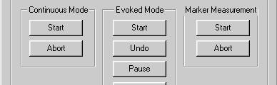
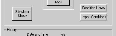
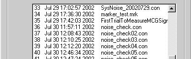
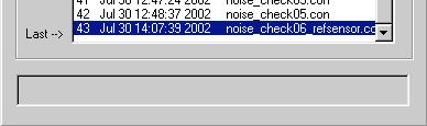
22 1.18 MEG Marker Positioning The dialog to estimate the positions of the MEG marker coils will appear. Another dialog to choose the marker coil measurement file will be opened upon clicking the Search button. After selecting the marker coil measurement file, the estimation starts upon clicking the Execute button. The result of the estimation is graphically shown on the dialog. Once the estimation is executed with a certain file, the result is stored in the file automatically. Load button can call the previously estimated result and the user doesn t need to execute the second estimation. If the users have more than one marker coil measurement file for the same session, the users may compare values. Press the Compare button. The users will be asked to load the second file. The differences between the localizations will be presented numerically and may also be presented graphically. If the answer is yes to the display, circles will represent the first/current file, and crosses will represent the second file. 2) Execute the localization command. 1) Make sure the estimation parameters are correct. Number of Markers should match the number of working sensors. Reference Channel is not used. Averaging Count should be 16. Trigger Threshold should be around ) Review the results of the localization. In particular, examine the GOF (goodness of fit) of the estimations (these should ideally be above 99%). The locations of the coils are displayed in those three directions. 21

23 22

24 1.19 Print... The general print dialog will appear. The screen shot of the window of Meg Laboratory can be printed by this command Print Preview The general print preview window will appear and the user can confirm the result of the printing on the screen Print Setup... The general print setup dialog will appear Exit Every MEG data file will be closed and Meg Laboratory is exited. 23

25 2. Acquis If the PC on which Meg Laboratory installed doesn t have the connection to the DAQ PCs and SQUID electronics, this menu option will not appear/exist. 24

26 2.1 System Definition System Scale The System Scale Setup dialog will appear. Here, the user can set the number of the DAQ PCs, the number of A/D boards installed on each DAQ PC, the number of the channels on an A/D board, and the number of the SQUID electronics. 25

27 2.1.2 Channel Definition The channel definition dialog will appear. The user can check or modify the type, position, and direction of each sensor and assign the names to the optional channels on the dialog. 26

28 2.2 Auto Tuning Setup Usually, this command is only used upon the initial installation process or in the regular maintenance process. The user must not use without the advices of the service support. The dialog to set the mode of the auto-tuning and the parameters for tuning will appear. There two modes of the auto-tuning: Full-tuning and Voffset-tuning. Full-tuning adjusts the two parameters of the SQUID sensors: bias current and offset voltage. Voffset-tuning adjusts only the offset voltage. 2.3 Auto Tuning The command tunes the parameters of all the SQUID sensors automatically. Before the MEG measurement, the user must execute this command. 27

29 2.4 Manual Tuning Usually, this command is only used upon the initial installation process or in the regular maintenance process. The user must NOT use without the advice of the service support. The SQUID electronics are fully controlled directly on the dialog. 2.5 DC offset Tuning This command is not implemented. 28

30 2.6 File Usually, the commands in this category are only used upon the initial installation process or in the regular maintenance process. The user must NOT use without the advice of the service support. The two parameters of the SQUID sensors, bias current and offset voltage, can be saved to a file and loaded from the file by the commands in this category Load The settings of the two parameters of the SQUID sensors (bias current and offset voltage) are stored in a file and thus can be called and set to the SQUID electronics by this command. The dialog to select the file to be opened will appear Save As The current settings of the two parameters of the SQUID sensors (bias current and offset voltage) can be saved to a file by this command. The dialog to name the file to be saved will appear Load Init File This command enables the user to reset the initial settings for the two parameters of the SQUID sensors (bias current and offset voltage) back to their initial state which was stored by the command Save Init File. 29

31 2.6.4 Save Init File The current settings for the two parameters of the SQUID sensors (bias current and offset voltage) can be saved as an initial state. To recall the initial state, the command Load Init File should be executed Save As Text File To analyze the parameters of the SQUID sensors (bias current and offset voltage) this command exports the current settings of the parameters to a text file. 30

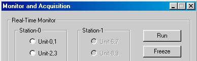
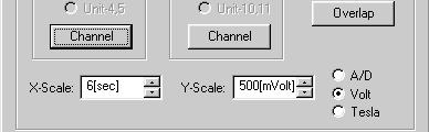
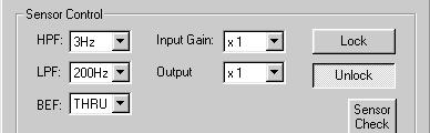
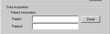
32 2.7 MEG Measurement The dialog controlling the DAQ PCs and the SQUID electronics will appear. Every recording of data is executed in this dialog. 31

33 2.8 Options The Measurement Options dialog will appear. The user can choose the behavior of the SQUID electronics upon launching Meg Laboratory on the dialog. The settings for the default file extension of the MEG data files in every mode can be changed, but this is NOT recommended. Other trivial settings relating to data acquisition can be changed in this dialog. 2.9 Control Panel This command is not available ReBoot DAQ This command reboots all the DAQ PCs remotely. 32

34 2.11 Shutdown DAQ This command shuts-down all the DAQ PCs remotely Maintenance Abort DAQ The command forces a termination of the software for the real time monitors on each DAQ PC. 33

35 3. Edit This menu appears only when MEG data files are opened. 3.1 Undo The command removes the effect of the previous command in the category of Edit and returns the data to the previous state. When this command is executed, the dialog confirming the operation will appear. 3.2 Cut This command is not available for this version. 3.3 Copy This command is not available for this version. 34

36 3.4 Paste This command is not available for this version. 3.5 Comment The user can input comments for the data file. The history of the comments is also preserved. The comments can be imported from other MEG data files. 35

37 3.6 Patient Info The user can input or modify the information of the patient. The information can be imported from other MEG data files or MRI data files. 3.7 Channel Info The channel definition dialog will appear. The user can check or modify the type, position, and direction of each sensor and assign names to optional channels in the dialog. 36

38 3.8 Macro Command The Macro command dialog will appear. The user can define a sequence of the commands in the Edit category; which is frequently used as a macro. The defined macro can be executed in the dialog. The commands that can be used in a macro are: HPF, LPF, BPF, BEF, Customized Filter, Moving Averaging, Baseline Correct, Absolute, Multiply, Power, and Channel Math. Operation. 37

39 3.9 HPF The High Pass Filter dialog will appear. The user can set: the cut-off frequency of the filter, window type, width of the digital filter, and the specific channels to be filtered. The frequency response of the filter can be checked graphically. 38

40 3.10 LPF The Low Pass Filter dialog will appear. The user can set: the cut-off frequency of the filter, window type, width of the digital filter, and the channels to be filtered. The frequency response of the filter can be checked graphically BPF The Band Pass Filter dialog will appear. The user can set: the cut-off frequency of the filter, window type, width of the digital filter, and the channels to be filtered. The frequency response of the filter can be checked graphically. 39

41 3.12 BEF The Band Elimination Filter dialog will appear. The user can set: the cut-off frequency of the filter, window type, width of the digital filter, and the channels to be filtered. The frequency response of the filter can be checked graphically Customized Filter The user can apply the original FIR filter to the data by this command. The filter should first be defined in text file format. The filter is expressed by the following formula. y(n) = N 1 k= 0 x(n k)h(k) where x and y are input and output of the filter, respectively, h is the transfer function. h determines the characteristics of the filter Moving Average The Moving Average dialog will appear. The point width, method of calculation of average, and the specific channels applied moving average can be selected in this dialog. The software can apply moving average to the digitized signals to smoothen out the signal s fluctuation. Given a sequence {a i } N i=1, an n-moving average is a new sequence {s i } N-n+1 i=1 defined from the a i by taking the average of subsequence of n terms, s i = 1 n i+n 1 j= i a j. So the sequence S n giving n-moving averages are 40

42 S 2 = 1 2 (a 1 + a 2, a 2 + a 3,..., a n 1 + a n ) S 3 = 1 3 (a 1 + a 2 + a 3, a 2 + a 3 + a 4,..., a n 2 + a n 1 + a n ) and so on. 41

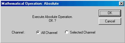
43 3.15 Baseline Correct The Baseline correct dialog will appear. This command corrects the difference in the offset of each channel by subtracting the average value for a certain time period from the sum of the original signal. The time region for the calculation of the average and optional functions can be selected in this dialog. The user can apply slope adjustment to compensate the linearly increasing/decreasing tendency of the digitized signal. This function is called slope fit. The algorithm of the slope adjustment approximate the signal by a linear function and then subtract the linear function from the original signal. If the measured signal is contaminated by periodical noise, the software can remove the noise using the noise template technique Absolute This command calculates the absolute value of the data for each channel at every time slice and replaces the results of the original signal. The Mathematical Operation: Absolute dialog will appear and the user can select whether all the channels should be applied to the calculation or only selected channels. 42

44 43

45 3.17 Multiply This command multiplies a given value of the data for each channel at every time slice. The results of the calculation will replace the original data. The Mathematical Operation: Multiply dialog will appear and the user can select either all the channels to be calculated/multiplied or only selected channels Power This command calculates certain values to the Nth power to the values at every time slice of each channel. The Mathematical Operation: Power dialog will appear. N will be the given value to be multiplied. The user can select either all the channels to be multiplied or only selected channels. 44

46 3.19 Channel Math. Operation The commands in this category calculate operations between data of multiple channels and then overwrite the existing data of a channel with the result of the calculations. 45

47 Maximum This command compares the values of the selected channels at every time slice and creates a new waveform by extracting the maximum value. The unit of measurement for the data can also be selected as either A/D or Tesla. This means that the user can select whether the data should be calibrated before operation, or not. The channels to be calculated and the overwritten channels can be selected as either Source Channel or Target Channel, respectively Minimum This command compares the values of the selected channels at every time slice and creates a new waveform by extracting the minimum value. The unit of measurement for the data can also be selected as either A/D or Tesla. This means that the user can select whether the data should be calibrated before operation, or not. The channels to be calculated and the overwritten channels can be selected as either Source Channel or Target Channel, respectively. 46

48 Average This command calculates the average values of the selected channels at every time slice and creates a new waveform. The unit of the data can be calculated in either A/D or Tesla. This means that the user can select whether the data should be calibrated before operation, or not. The channels to be calculated and the overwritten channels can be selected as either Source Channel or Target Channel, respectively Weighted Average This command calculates the weighted average of all the channels at every time slice and overwrites the data with the result. A text file which has a list of the weight coefficients (which we call Weight File) should be prepared before executing the command. The Weight File and the overwritten channels are selected in the dialog. The unit of measurement for the data can be selected as either A/D or Tesla. This means that the user can select whether the data should be calibrated before operation, or not. 47

49 RMS This command calculates the Route Mean Square of a specific set of the channels at every time slice and overwrites the data with the result. The channels to be calculated and the overwritten channels can be selected as either Source Channel or Target Channel, respectively File Math. Operation The commands in this category calculate between the active file and the other files. The result overwrites the active file. 48

50 Add The data from a certain file is added to the data in the active file one channel at a time. The result of the addition overwrites the active file. The user can then select the file and the channels to be added. The sampling rate, data length, and number of the channels should be identical between the two files Subtract The data from a certain file is subtracted from the data in the active file one channel at a time. The result of the subtraction overwrites the active file. The user can then select the file and the channels to be subtracted. The sampling rate, data length, and number of the channels should be identical between the two files Concatenate The data from a certain file is linked with the data in the active file. The user can then select the file and the channels to be concatenated. The two files must have the same number of channels and have been recorded at the same sampling rate. 49

51 3.21 Extract The data can be cut out between two given time slices. Start time and End time can be set in the dialog. The data in the unselected region will be lost Thin out This command reduces the sampling point in the data. The data will be extracted only at every x time slice where x is the given value for Thinout Count. The data at the nonextracted time slices will be lost. 50

52 3.23 Patch This command interpolates the data between two time slices by a linear patch or a spline patch. The Temporal Patch dialog will appear. The user can set the region and the channels to be patched and then select the patch type on the dialog Forward Problem The existing data of each channel at the selected time slice will be replaced by the theoretical magnetic field calculated from the estimated current dipoles at that moment. This command is selectable only when the user picks the time slice at which the estimated dipoles are registered. The calculation of the theoretical magnetic field distribution from the electric current is called forward problem of electromagnetism. On the other hand, pursuing the electric current distribution based on the observed magnetic field is called inverse problem of electromagnetism. 51

53 3.25 Noise Reduction The Noise Reduction using Reference Channels command will appear upon selecting this command. This only applies if the system is equipped with the magnetic sensors for the environmental magnetic noise. In addition, these signals along with the MEG signals need to be acquired. The noise contaminating the MEG signals can be reduced using the signals from the circumstance for the reference. 52

54 3.26 Averaging The data recorded in the continuous mode or in the evoked mode with raw data can be applied in the offline averaging operation. Two dialogs, Offline Averaging [Main] and Offline Averaging [Trigger List], will appear. This command can only be selected if the data from the active file has not been averaged. 53

55 4. MRI Meg Laboratory needs the image data that shows the morphology of the brain for the investigation of the magnetic source. The image data is mainly provided by an MRI system. All commands in this category treat the morphological data from MRI systems as the magnetic source estimation. 4.1 Create MRI File from DICOM-3 file The dialog to select the set of the DICOM files of the MRI data will appear. The selected files are combined and transformed to a single file in the Meg Laboratory MRI format. The extension of the transformed file is *.mri. After choosing the set of the original data files in DICOM format, the dialog to name the created MRI data file will appear. 4.2 Create MRI File from pixel data The dialog to create the Meg Laboratory MRI data format file from the set of the general image files will appear. To make the MRI data file (created by this command equivalent to the file from the DICOM format file), it is necessary to input the information of the patient, the binary format of the original data files, slice features of the set of the original files, the pitch of the pixels, etc. After setting the parameters in the dialog, the dialog to name the created MRI data file will appear. 54

56 4.3 Create MRI File from digitizer data This command creates an MRI data file in Meg Laboratory MRI data file format with the extension of *.mri from the EMSI data files acquired by the 3D digitizer of Polhemus, such as FASTRAK or ISOTRAK. The dialog to input the patient information, select the filename of head shape file and marker coil file from EMSI, and assign the coordination system will appear. The head shape file and the marker coil file have the extensions of *.hsp and *.elp, respectively. After setting the parameters, the dialog to name the created MRI data file will appear. 4.4 Setup Head Coordinate System This command assigns the head coordination system to the existing MRI data file in Meg Laboratory format. The dialog to select the MRI data files in Meg Laboratory format will appear. After choosing the filename of the MRI data file, the dialog to set the coordination system will be opened. The information of the coordination is attached to the MRI data file upon clicking OK button on the dialog. 55

57 4.5 MRI Filename This command creates a link between the active MEG data file and the MRI data file created by one of the commands described in previous sections. The Open MRI file dialog will appear. Next, select the MRI data file of the corresponding subject to the active MEG data file. After selecting the MRI data file, the dialog to confirm the subject s name and ID will appear before opening the MRI file. If the user doesn t have the MRI data of the corresponding subject to the active MEG data file, the virtual MRI data can NOT be selected. Once the link between the MEG and MRI data file has been created, the file path from the MEG data file to the MRI data file is stored in the MEG file. The user doesn t need to make the link more than once, unless the relative location of the MRI file is changed. The option of Without MRI can be selected, if the user wants to delete the link. 56

58 4.6 Pick MRI Marker The MRI Operation dialog will appear upon executing this command. The user can pick up the position of the MRI Markers and confirm the assigned positions. Once this command is executed for a certain MRI data file, the information about the positions of the markers is stored in the MRI data file automatically. The user doesn t need to assign the locations more than once. If the MRI data file is not linked to the active MEG file, this command cannot be selected. 57

59 4.7 MEG Marker Positioning The dialog to estimate the positions of the MEG marker coils will appear. Another dialog to choose the marker coil measurement file will also open. After selecting the marker coil measurement file, the estimation starts upon clicking Execute button. The result of the estimation is graphically shown on the dialog. Once the estimation is executed with a certain file, the result is stored in the file automatically. Load button can call the previously estimated result and the user doesn t need to execute the second estimation. 4.8 MRI-MEG Matching This command can be selected after assigning the position of the MRI markers and estimating the positions of the MEG markers. The MRI Operation dialog will appear upon executing this command. The MEG coordination system and the MRI coordination system will be matched upon clicking the Do Matching button and the error between two systems will then be displayed. The markers to be used for matching can also be selected by the user in the dialog. Basically, all five markers should be used for matching. 1) If any of the marker coils are not to be used, deselect them (uncheck the box next to it). 2) Then press the Do Matching button. 3) The results of the matching will be displayed, along with the error around each marker. If any of the coils shows an excessive error, deselect it and perform the matching again. 58

60 5. Analysis 59

61 5.1 Sphere Model The source analysis by Meg Laboratory assumes that the brain is a spherical conduction. The dialog to fit a sphere to the brain graphically will appear. The user can assign a spherical model to the brain automatically in the dialog. Manual assignment is also available. The position and the size of the sphere can be adjusted by drawing a circle over the MR image, or by numerical input. Once this command is executed for a certain MRI data file, the information about the spherical model is stored in the MRI data file automatically. The user doesn t need to assign the sphere again. If the MRI data file is not linked to the active MEG file, this command cannot be selected. A circle is drawn by dragging over the MRI image. The sphere is determined by clicking this button. The parameters of the sphere can be adjusted numerically. 60

62 5.2 Dipole Fitting After the active MEG data file is linked to the MRI data file and both of the coordination systems of MRI and MEG are matched to each other and the spherical model is assigned to the MRI data, this command is selectable. The dialog to fit one or two theoretical current dipoles to the observed magnetic field distribution at the selected time slices will appear upon selecting this command (for multiple dipoles, or more than two dipoles, use the Multi Dipole Fitting command which functions the same as Dipole Fitting). Choose a single time slice, or a series (to select a series, SHIFT-click and draw a box on the waveform viewer over the time period). If a series is chosen, all dipoles after the first are localized starting from the previous location, rather than randomly. Displays the channels currently being used for dipole fitting Fitting Parameters: Moving dipole (location, orientation, and intensity can vary) Fixed dipole (orientation and intensity can vary) Moment Free dipole (intensity can vary) Initialization: Random, Closest Entry (starting point is from the latency with a dipole Note, if a series is fit, all time points but the first operates as Closest Entry), Manual Set select a starting point manually on the MR image. Used for bilateral dipoles (e.g. auditory response). First, localize response in one hemisphere. Then, localize response in the other hemisphere. Select all MEG channels, check the bilateral option, and Estimate again. Once a dipole has been fit, GOF, location, orientation, and intensity information is filled in. 61

63 5.3 Multi Dipole Fitting After the active MEG data file is linked to the MRI data file and both of the coordination systems of MRI and MEG are matched to each other and the spherical model is assigned to the MRI data, this command is selectable. The dialog to fit one or more theoretical current dipoles to the observed magnetic field distribution at the selected time slices will appear upon selecting this command. 62

64 5.4 Lead Field Reconstruction After the active MEG data file is linked to the MRI data file and both of the coordination systems of MRI and MEG are matched to each other and the spherical model is assigned to the MRI data, this command is selectable. The dialog to construct the current dipole array by the lead field method on the specific plane will appear upon selecting this command. 63

65 5.5 Manual Dipole Fitting After the active MEG data file is linked to the MRI data file and both of the coordination systems of MRI and MEG are matched to each other and the spherical model is assigned to the MRI data, this command is selectable. The user can define the theoretical current dipoles manually in the dialog which appears upon selecting this command. 64

66 5.6 Arrange MSI Entries The theoretical current dipoles estimated by the commands described in the previous sections are registered in the MSI list. The commands in this category sort the registered magnetic sources at a specific time slice in the specific order Right to Left The magnetic source entries are sorted by the spatial positions from right to left from the view point of the subject Left to Right The magnetic source entries are sorted by the spatial positions from left to right from the view point of the subject Anterior to Posterior The magnetic source entries are sorted by the spatial positions from subject s anterior to posterior Posterior to Anterior The magnetic source entries are sorted by the spatial positions from subject s posterior to anterior Superior to Inferior The magnetic source entries are sorted by the spatial positions from subject s superior to inferior. 65

67 5.6.6 Inferior to Superior The magnetic source entries are sorted by the spatial positions from subject s inferior to superior by Intensity in descending order(+) The magnetic source entries are sorted by the intensity of the dipole in descending order by Intensity in ascending order (-) The magnetic source entries are sorted by the intensity of the dipole in ascending order. 66

68 5.7 Medical Opinion The user can make notes in the comment field of each estimated dipole as medical opinion. The dialog to select dipoles will appear upon executing this command. The dipoles to which the user attach the comments can be selected by clicking the item in the list of MSI. The user can also extract the dipoles from the list in accordance with a certain condition. After clicking the OK button, the comment field will be appear. The user can make a comment for the selected dipoles within 80 characters. 67

69 5.8 Delete MSI Entry The commands in this category delete the entries of magnetic source from the MSI list Delete current Entry All the magnetic entries at the selected time slice will be deleted Delete series Entries All the magnetic entries in the selected series of the time slices will be deleted. 68

70 5.8.3 Delete specified Entries The MSI list will appear upon selecting the command. The user can select the specific magnetic source to be deleted from the list Delete multiple Entries If there are multiple MSI entries on the selected time slice, this command can delete the entries at once. 69

71 5.8.5 Delete all Entries All magnetic source entries will be deleted. 5.9 Book Mark The user can put a mark called book mark on any time slice by this command. There are two types of book mark. One is retained type which is preserved with the data in the file upon saving. The other is temporal type which is not saved in the file and vanishes upon closing the file. The user can label and make a comment for each book mark. 70

72 5.10 Entry Book Mark from MSI The user can set a book mark to the time slice at which a dipole is estimated. The dialog to select dipoles will appear upon executing this command. The dipoles to which the user set the book mark can be selected by clicking the item in the list of dipoles. The user can also extract the dipoles from the list in accordance with a certain condition. After clicking the OK button, the dialog selecting the type of book mark between retained and temporal will be appear. 71

73 5.11 Delete Book Mark Entry Delete current Entry The book mark at the selected time slice will be deleted Delete series Entries The book marks in the selected series of the time slices will be deleted Delete specified Entries The list of the book marks will appear upon selecting the command. The user can select the specific book marks to be deleted from the list Delete all Entries All book marks will be deleted. 72

74 6. Tool 6.1 Statistics of Data Minimum, maximum, average, range, and standard deviation of the data for each channel can be displayed in the dialog. The channels that have the maximum range, the minimum range, the maximum standard deviation, and the minimum standard deviation are shown with their values. The grand average and the grand standard deviation is calculated through all the selected channels. The time region for the calculation can be selected. The resulting data is displayed with 16 channels per page. The information in the dialog can be exported to a text file from the File menu. The start time and the end time over which to calculate the statistics must be specified. 73

75 6.2 Statistics of MSI The spatial distribution of the location of the magnetic source in the MSI list will be shown in the dialog. The information in the dialog can be exported to a text file from the File menu. 74

76 6.3 Auto Correlation There are several correlation options built in to Meg Laboratory. A (bivariate) correlation is a statistical analysis that examines the relationship between two variables; if there is a strong predictive relationship between two variables either positive (e.g., if one rises, the other rises, like difficulty of a sentence and processing time), or negative (e.g., if one rises and the other falls, like loudness of a stimulus and time to perception) then there will be a strong correlation between the variables. The correlation functions in Meg Laboratory permit the examination of a sensor s relationship to itself over a variety of time ranges ( autocorrelation ), to another sensor over a variety of time ranges ( cross correlation ), to another sensor at only one time range ( correlation ), to all sensors at only one time range ( correlation map ), and to the analogous sensor from another file/condition at one time range ( file correlation ). Autocorrelation of data of a selected channel will be calculated upon selecting this command. Autocorrelation is the correlation of one sensor to itself. The result will be shown in the dialog. 1) Enter the start time and end time of the range over which to perform the correlation. 2) Make sure the appropriate channel is specified. 3) Press Display. 75

77 6.4 Cross Correlation Cross-correlation of data of two selected channels will be calculated and the result will be shown in the dialog. The relationship between two different sensors is examined over varying time intervals to see if a predictive relationship exists between an earlier time and a later time. 1) Enter the start time and end time of the range over which to perform the correlation. 2) Make sure the appropriate channels are specified. 3) Press Display. 6.5 Correlation The user must select two channels in the waveform viewer before executing this command. The command calculates the correlation coefficient of the two channels and shows the result in the dialog. 76

78 6.6 Correlation Map The user must select one channel in the waveform viewer before executing this command. The command calculates a cross-correlation coefficient between the selected channel and the other channels. It means that a cross-correlation coefficient with the selected channel is assigned to each channel. The set of cross-correlation coefficients is exported to a new MEG data file which has just one time slice. The contour map of the cross-correlation coefficients can be shown in the created MEG data file. 6.7 File Correlation A dialog to select a MEG data file will appear. The Cross-correlation coefficient between the data of the active file and the selected file is calculated. The two files must have the same data attributes (sensor configuration, sampling rate, data length, etc.). 77

79 6.8 t-test 78

80 6.9 Time-Integral All the data of each channels are integrated along the temporal axis. The result is shown in the manner of the contour map. The time region for integration can be selected. The way to integrate can be selected from Summation of Signed, Summation of Absolute, and Root of Square-Summation. 79

81 6.10 FFT Amplitude The Amplitude Spectrum dialog will open. Select the channels to be calculated. The user can then select Start Time, Number of points, Window Type, and Scale for the calculation. Amplitude Spectrum is calculated by FFT and the result can be shown graphically in the dialog upon clicking the Display button. It can be exported to a text file. Averaging along the temporal axis can be applied by the command in the Option menu. 1) Select the appropriate channels (up to 32); these should be entered separated by a comma; or, by pressing the Select Channel button, the channel map is opened (see 8.19). 2) Enter the starting time (since the FFT is calculated over a period of time, and not at a single point, this requires some forethought). 4) Press Display. 3) Choose the number of points to be used, using the pull-down menu. This is similar to choosing the end time; the more points are chosen, the more accurate the result however, some averaged files, particularly those with lower sampling rates, will not be able to support many of the options. The users can see that the amount of time included does depend on the sampling rate and the data length. Frequency bands are listed along the bottom. 80

82 6.11 FFT Power The Power Spectrum dialog will open. Select the channels to be calculated. The user can then select Start Time, Number of points, Window Type, and Scale for the calculation. Power Spectrum is calculated by FFT and the result can be shown graphically in the dialog upon clicking the Display button. It can be exported to a text file. Averaging along the temporal axis can be applied by the command in the Option menu. 81

83 6.12 FFT Phase The Phase Spectrum dialog will open. Select the channels to be calculated. The user can select Start Time, Number of points, Window Type, and Scale for the calculation. Phase Spectrum is calculated by FFT and the result can be shown graphically in the dialog upon clicking the Display button. It can be exported to a text file. Averaging along the temporal axis can be applied by the command in the Option menu. 82

84 6.13 FFT Map The amplitude and phase components calculated for every sensor by FFT at the specific frequency or the amplitude components in the specific band are shown in the manner of the contour map upon clicking the Display button. 83

85 6.14 Time-FFT Map The temporal transition of the FFT Map is calculated and the result is exported to another file in the MEG data file format. 84

86 7. Property The commands in this category show the attributes of the MEG data file. Every command produces another dialog that displays the information. The information of the dialog is then exported to a text file. 7.1 Basic Info The information about the MEG system by which the MEG data file was recorded will be shown. It contains system name, model name, system ID, version of the software, the number of the channels, the time when the file was created. 7.2 Patient Info The information about the patient, patient ID, patient s name, birthday, sex, and dominant hand, will be shown. 7.3 History Info The history of the user s operations for the data file will be shown. 7.4 Channel Info The sensor type, the locations and directions of each sensor in the MEG coordination system will be shown. 7.5 Calibration Info The sensor type, sensitivity, and offset of each sensor will be shown. 85

87 7.6 FLL Info The parameters of SQUID sensor, bias current and offset voltage, will be shown for each sensor. 7.7 Amp and Filter Info The gain of amplifiers and the cut-off frequency of the filters will be shown. 7.8 Acquis Condition Info For the data file recorded in continuous raw data acquisition mode, sampling rate, acquisition time, actual time, and trigger mode will be shown. For the data file recorded in evoked average data acquisition mode, sampling rate, frame length, pre-trigger length, post-trigger length, condition of level rejection, averaged count, actual averaged count, rejected count, and trigger conditions will be shown. 7.9 Trigger Event Info The information about the trigger event will be shown MRI Info The filename of the MRI data file linked to the MEG data file, the information of conductor model fit to the MRI data, head coordination system information will be shown. The conductor model information is displayed in the MRI coordination system MRI-MEG Matching Info The information about the location of markers and transformation between MRI coordination system and MEG coordination system will be shown. The filename of the linked MEG maker file, the position of MEG and MRI makers described in MRI coordination system, transform matrix between the two coordination system, the distance between two of the five markers, and the deviation between the position of MRI markers and the transformed position of MEG markers are included Measured Data Info The data at the selected time slice will be shown in Tesla, A/D, or Volt units. 86

88 7.13 Magnetic Source Info The information of the estimated theoretical magnetic sources will be shown. The location, direction and intensity of the current dipoles, and the date and time of when the magnetic source was recorded is included Book Mark The information of the book marks will be shown Save Any Properties As All information displayed by the commands in this category is exported to a text file. The user can select the information to be exported on the dialog that appears upon executing this command. 87

89 8. View An MEG data file contains many kinds of information - not only the data from the sensor. The commands in this category are used for selecting the information displayed on the screen and changing the arrangement in the data window. 8.1 Toolbar This command toggles the toolbar on and off. 8.2 Status Bar This command toggles the status bar on and off. 88

90 8.3 Layout The main window to display the MEG data file has five zones. They are: title, waveform viewer, isofield contour map, MRI viewer, and magnetic source report. The commands in this category switch the arrangement of the five zones in the window Standard Layout The title, waveform viewer, isofield contour map, MRI viewer, and magnetic source report are arranged as the following figure: 89

91 8.3.2 Waveform Leftside The title, waveform viewer, isofield contour map, MRI viewer, and magnetic source report are arranged as the following figure: Waveform Upside The title, waveform viewer, isofield contour map, MRI viewer, and magnetic source report are arranged as the following figure: 90

92 8.4 Standard 3-View Title, waveform viewer, isofield contour map, and MRI viewer are shown. This set is called the standard 3-view arrangement. 8.5 Standard 4-View Title, waveform viewer, isofield contour map, MRI viewer, and magnetic source report are shown. This set is called the standard 4-view arrangement. 8.6 Title View The items for the title zone are the patient information, the filename of the MEG data file, and the condition of the acquisition. The commands in this category switch the information to be displayed in the title zone Show The display of the title zone can be switched on and off by this command Patient Info 91

93 The display of patient information in the title zone, patient name and patient ID, can be switched on and off by this command File Extension The display of the file extension in the filename in the title zone can be switched on and off by this command Acquis Condition The display of the condition of the acquisition, which contains the measurement date and time, the setting of the filters, the sampling rate, and average count, can be switched on and off by this command. 92

94 8.7 Waveform View Full Size Only the waveform viewer and the title zone are shown on screen upon executing this command Show The display of the waveform viewer can be switched on and off by this command. 93

95 8.7.3 Display Range Display Range dialog will appear upon executing the command. The time slice to be operated can be selected numerically. The user can display the range, both in x-axis and y-axis, in the waveform viewer. If the user input too narrow range to display, the values are modified automatically EEG scale The scales of x and y axis of waveform viewer are changed to the appropriate expression for the EEG signals by this command Overlap The data of every selected channel is displayed in overlap mode. The graph in this mode is sometimes called a butterfly plot. 94

96 8.7.6 Parallel The data of every selected channel is displayed in parallel Gridmap The data of every channel is displayed in gridmap mode. 95

97 8.7.8 Tesla The command changes the unit of y-axis to Tesla. The unit is transformed from A/D to Tesla using the information for the gain of amplifiers and the sensitivity of each SQUID sensor A/D The command changes the unit of y-axis to A/D. A/D is the original unit of the data acquired by data acquisition system. This unit is converted to Tesla based on the information from the gain of amplifiers and the sensitivity of each SQUID sensor Voltage The command changes the unit of y-axis to Volts RMS only The Route Mean Square of all signals for the selected channels is calculated at every time slice. The RMS waveform is only displayed on the waveform viewer. This command is effective only when the waveforms are displayed in overlap mode. 96

98 97

99 RMS also The Route Mean Square for all the signals of the selected channels is calculated at every time slice. The RMS waveform and the selected signals are displayed together on the waveform viewer. This command is effective only when the waveforms are displayed in overlap mode. 98

100 Splitter Waveform The waveform viewer can be separated into two parts to show the data for the two different sets of channels. For example, if the users wanted to view left- and right- hemisphere activations simultaneously but not superimposed, the users could use this command. The commands in this category affect the second set in the waveform viewer Full Size The command makes the second set of the data occupy the waveform viewer. 99

101 Show The display for the second data set in the waveform viewer can be switched on and off by this command Overlap The data for every selected channel in the second data set is displayed in overlap mode. The graph in this mode is sometimes called a butterfly plot Parallel The data for every selected channel in the second data set is displayed parallel Tesla The command changes the unit of y-axis to Tesla for the second data set display. The unit is transformed from A/D to Tesla using the information of the gain of amplifiers and the sensitivity of each SQUID sensor A/D The command changes the unit of y-axis to A/D for the second data set display. A/D is the original unit of the data acquired by data acquisition system. This unit 100

102 is converted to Tesla based on the information of the gain of amplifiers and the sensitivity of each SQUID sensor Voltage The command changes the unit of y-axis to Volts for the second data set display Select Channel Upon executing this command, Select Channel dialog will appear to select the channels for the second data set display. (See 8.19) 101

103 Background The display of the axes, grid lines, and labels in the waveform viewer (in overlap and parallel modes), can be switched on and off by this command. In the case of gridmap mode, the display for the channel number, scales, outline of the head, and the indication of left and right, can be switched on and off by this command Outline The display for the outline of the patient s head in the waveform viewer (in gridmap mode) can be switched on and off by this command. This command is effective only when the waveforms are displayed in gridmap mode Epoch Frame The time frames of each epoch to be extracted for averaging are displayed on waveform viewer by this command X-Cursor The cursor for x-axis can be switched on and off with this command. 102

104 Y-Cursor Show The cursor for y-axis can be switched on and off with this command. This command is only effective when the waveforms are displayed in overlap mode. 103

105 Mouse Cursor The display of the value at the position indicated by clicking on the waveform viewer can be switched on and off by this command. This command is effective only when the waveforms are displayed in overlap mode Maximum The display of the maximum value of the selected data at the time slice indicated by the x-cursor can be switched on and off with this command. This command is only effective when the waveforms are displayed in overlap mode. 104

106 Minimum The display of the minimum value for the selected data at the time slice (indicated by the x-cursor) can be switched on and off with this command. This command is only effective when the waveforms are displayed in overlap mode RMS The display of the RMS value for the selected data at the time slice (indicated by the x-cursor) can be switched on and off with this command. This command is only effective when the waveforms are displayed in overlap mode Book Mark This command switches on/off the display of the bookmarks on waveform viewer Non-MEG Channels on Gridmap The display of Non-MEG channels on the waveform viewer, in gridmap mode, can be switched on and off with this command. This command is only effective when the waveforms are displayed in gridmap mode. 105

107 Reference Waveform The user can view data from two or more MEG data files simultaneously in the same window. This command brings up the dialog to choose two or more MEG data files. This command will NOT work if files are of different lengths, and if a file is not baseline-adjusted. Files viewed with this command should already be processed (e.g., baseline-adjusted). To view files either overlapping or parallel, use the Add button. To remove files from view, use the Delete button. To insert a reference waveform within the list already created, use the Insert button. 106

108 8.8 Contour Map View Full Size Only the isofield contour map and the title zone are shown on the screen upon executing this command Show The display of the isofield contour map can be switched on and off with this command Measured Contour An isofield contour map based on the observed magnetic fields at the selected time slice is shown singularly. 107

109 8.8.4 Measured + Theoretical Contour The Two isofield contour maps, based on the observed magnetic fields and the theoretical magnetic fields calculated from the estimated current dipoles at the selected time slice, are shown. If there is no entry of MSI at the selected time slice, the theoretical map isn t shown Measured + Theoretical + Residual Contour The Three isofield contour maps, based on the observed magnetic fields, the theoretical magnetic fields calculated from the estimated current dipoles, and the residual magnetic fields in the estimation, are shown. If there is no entry of MSI at the selected time slice, the theoretical and residual maps aren t shown. 108

110 8.8.6 Auto The software chooses one of the three modes automatically which are: Measured, Measured + Theoretical, and Measured + Theoretical + Residual. These are based on the area for the isofield contour map. If there is sufficient space to display the three contour maps, and the theoretical current dipoles are estimated for the selected time slice, the software will choose the Measured + Theoretical + Residual mode Color Contour The contour map is only described by lines. Two colors are used on the contour map to express the rising fields from the patient s head and the sinking fields into the head. 109

111 8.8.8 Line Contour The contour map is only described by lines. Two colors are used in the contour map to express the rising fields from the patient s head and the sinking fields into the head. The brightness of the color of the lines is changed by the intensity of the field assigned to the lines. The less intensity is represented by the darker lines Gradation Contour The contour map is filled by two tone colors. The higher intensity area is filled by the stronger color. 110

112 Line Gradation Contour The contour map is filled by two tone colors. The higher intensity area is filled by the stronger color. The border lines between the two adjacent areas are also displayed Auto Gain If this option is selected (checked), the step value between lines are adjusted automatically to fit the amplitude of the wave. If this option is deselected, the scale of the contour map will remain constant, unless it is adjusted manually. 111

113 Whole Area When this option is checked, the contour map for the whole area is displayed without reference to the selected channels. If this option is not checked, the contour map only for the adjacent area of the selected channels is displayed Background The display of the title, the scale, and the indication of left and right can be switched on and off with this command Outline The display of the outline of the patient s head in the contour map can be switched on and off with this command Channel Position The display of the grid representing the position of each SQUID sensor can be switched on and off with this command. 112

114 Channel Number The display of the channel number beside the corresponding grid on the contour map can be switched on and off with this command. This command is only effective when the channel positions are displayed. 113

115 8.9 MRI View The MRI viewer can display not only the MR image but also the assigned sphere model, the arrangement of the sensor array, the estimated theoretical current dipoles, etc. The command in this category treats the spatial information to be displayed in the MRI viewer in the manner of the projection from the three orthogonal directions Full Size Only MRI viewer and title zone are shown on screen upon executing this command Show The display of the MRI viewer can be switched on and off with this command Axial View The display of the axial view in the MRI viewer can be switched on and off with this command. 114

116 8.9.4 Coronal View The display of the coronal view in the MRI viewer can be switched on and off with this command Sagittal View The display of the sagital view in the MRI viewer can be switched on and off with this command Background The display of the title, the slice number, and the indication of left / right and anterior / posterior can be switched on and off with this command MR-Image The display of the MRI data linked to the active MEG data file can be switched on and off with this command MEG Sensor The display of the arrangement of the sensor array can be switched on and off with this command MEG Marker The display of the positions for the MEG markers in the MRI viewer can be switched on and off with this command MRI Marker The display of the positions for the MRI markers in the MRI viewer can be switched on and off with this command Sphere Model The display of the sphere conductor model assigned to the MRI data can be switched on and off with this command. 115

117 Contour Map The display of the three dimensional contour map in the MRI viewer can be switched on and off with this command Dipole The display of the location and direction of the estimated theoretical current dipoles in the MRI viewer can be switched on and off with this command Coordinate Frame The display of the frame for the MRI coordination system can be switched on and off with this command Slice Position The display of the indication for the selected MRI slice can be switched on and off with this command Display All When this command is executed, all of the options described above will be displayed in the MRI viewer Link to Dipole #1 When this option is enabled, the slice including the location of the estimated theoretical dipole #1 is displayed in the MRI viewer, upon selecting the time slice at which there is an MSI entry Link to Dipole #2 When this option is enabled, the slice including the location of the estimated theoretical dipole #2 is displayed in the MRI viewer, upon selecting the time slice at which there are two or more MSI entries No Link to Dipole When this option is enabled, the displayed slice isn t changed even upon selecting a time slice at which there is an MSI entry. 116

118 Reference Dipoles The positions of the estimated dipoles in the other time slices can be displayed in the MRI viewer with this command. The dialog for selecting the dipoles to be displayed from the MSI list will appear upon executing the command. 117

119 Reference Dipoles of Other File The positions of the estimated dipoles in other MEG data files can be displayed in the MRI viewer with this command. This dialog sets the dipoles to be displayed. Another dialog to select the other MEG data file will appear upon clicking the Add button. After selection of the MEG data file, the MSI list of the selected file will appear. 118

120 8.10 MSI Report View MSI Report viewer is the numerical display of the theoretical current dipoles estimated for the selected time slice. The commands in this category change the characteristics of MSI Report viewer Full Size Only MSI Report viewer and title zone are shown on screen upon executing this command Show The display of MSI Report viewer can be switched on and off with this command MEG Coordinate The coordination system for the values of the positions and directions in the MSI Report viewer is changed to the MEG coordination system upon executing the command MRI Coordinate The coordination system for the values of the positions and directions in the MSI Report viewer is changed to the MRI coordination system upon executing the command Head Coordinate The coordination system for the values of the positions and directions in the MSI Report 119

121 viewer is changed to the head coordination system upon executing the command. The command is selectable only when the head coordination system is defined MSI Select View The user can mark the dipoles adapting to specific conditions regarding latency, GOF of estimation, intensity of the dipole, date and time for the estimation, comment text, and labels. The dialog to set the condition will appear upon executing the command. 120

122 8.12 Select View Format Show The display of the marks for the selected dipoles by MSI Select View in section 8.11 on both of Waveform View and MRI View can be switched on and off by this command Waveform View The display of the marks for the selected dipoles by MSI Select View in section 8.11 on Waveform View can be switched on and off by this command MRI View The display of the marks for the selected dipoles by MSI Select View in section 8.11 on MRI View can be switched on and off by this command Colored by Label The colors of the marks are determined by the label for each MSI entry by choosing this command Colored by Time The colors of the marks are determined by the time slice for each MSI entry by choosing this command. 121

123 Colored by GOF The colors of the markers are determined by the GOF of each MSI entry by choosing this command Colored by Intensity The colors of the markers are determined by the intensity of each MSI entry by choosing this command Colored by Time order The color gradation in accordance with the latency of each MSI entry is applied to the markers by choosing this command Colored by GOF order The color gradation in accordance with the GOF of each MSI entry is applied to the markers by choosing this command Colored by Intensity order The color gradation in accordance with the intensity of each MSI entry is applied to the markers by choosing this command. 122

124 8.13 Search Next This command can scan the dipole fulfilling the given condition along the lines of temporal axis. The dialog to set the conditions will be appeared upon selecting the command. When the OK button is clicked, the nearest dipole from the current time slice is indicated in Waveform View Select View All All conditions to select specific dipoles are canceled and all dipoles in the MSI entry is marked by choosing this command Series View The user can select two or more time slices in the specific time region by dragging the mouse on the waveform viewer while pressing SHIFT. The selected time region is filled by the different color from the other region on the waveform viewer. The software can treat the selected time slices as a series. The commands in this category are related to the series. 123

125 Show The display of the series can be switched on and off by executing this command Waveform View Every time slice at which the theoretical current dipoles are estimated in the series is indicated by the pin-like mark when this option is enabled MRI View The position of every dipole in the series is displayed on the MRI viewer when this option is enabled Contour Map Window The contour map at every time slice in the series is displayed on another window upon executing this command MR-Image Window This function has not been implemented yet. 124

126 8.16 Series View of All MSI The time slices in the time region including all estimated MSI are automatically selected as a series with this command. 125

127 8.17 Graphic Attribute The user can customize the appearance and the default settings of the data window by the commands in this category. 126

128 Frame Attribute The attributes related to the frame of the viewer can be changed in the dialog opened with this command. 127

129 Waveform Attribute The attributes related to the waveform viewer can be changed in the dialog opened with this command Contour Attribute The attributes related to the contour map can be changed in the dialog opened with this command. 128

130 MRI Attribute The attributes related to the MRI viewer can be changed in the dialog opened with this command Serial/Select View Attribute The attributes related to Serial view and Select view can be changed in the dialog opened with this command. 129

131 Initial View Attribute The initial state of each viewer and the options to be enabled upon opening the MEG data file can be set in the dialog opened with this command Init All Attribute All the settings of the attribute are returned to the initial state with this command Import All Attribute All the settings of the attribute are imported from the attribute file. 130

132 8.18 Associated windows The commands in the Tool or Property category will make another dialog. These dialogs are not modal and arrangement of the dialogs is controlled by the commands in this category Minimize The active dialog will be minimized Maximize The active dialog will be maximized Normalize The size of the active dialog will be reset to the initial size Close The active dialog will be closed. 131

133 Minimize others Dialogs other than the active one will be minimized Maximize others Dialogs other than the active one will be maximized Normalize others The size of dialogs other than the active one will be reset to the initial size Close others Dialogs other than the active one will be closed Minimize all All dialogs will be minimized Maximize all All dialogs will be maximized Normalize all The size of all dialogs will be reset to the initial size Close all All dialogs will be closed. 132

134 8.19 Select Channel The dialog to select the channels to be displayed on the waveform viewer will appear upon executing this command. This dialog is used for selection of the sensors when the Select Channel button on the other dialog is clicked. Click on channels above or below. Dragging is also effective. Choose from: Set mode: simply click on or draw a box around selected sensors. Shiftclick adds sensors, Ctrlclick removes them. Add mode: where every sensor clicked on is added. Delete mode: where every sensor clicked on is deleted. Toggle mode: where a click toggles the setting of selected sensors MSI Using Channel With this command, the channels whose data are used for the estimation of the theoretical current dipoles at the time slice are selected to be displayed on the waveform viewer. 133

135 9. Window 9.1 New Window This command opens another window of the same data file as the active file. 9.2 Cascade This command arranges the windows in cascade. 9.3 Tile Horizontal The windows on the screen are tiled horizontally. 9.4 Tile Vertical The windows on screen are tiled vertically. 9.5 Arrange Icons The minimized windows are arranged in order. 10. Help 10.1 About MegLaboratory... Copyright and the version information is displayed on another dialog with this comma 134