Spatial Analysis and Modeling (GIST 4302/5302) Guofeng Cao Department of Geosciences Texas Tech University

Transcription

1 Spatial Analysis and Modeling (GIST 4302/5302) Guofeng Cao Department of Geosciences Texas Tech University

2 Outline of Today Last week, we learned: Characteristics of spatial data Types of spatial data This week, we will learn: Representation of different types of spatial data in computers (databases) Commonly used operations

3 ArcGIS Desktop CDs Become available Version 10.1 Two steps: Activation. Important: the url listed on the CD wrap is wrong, please use this one instead: Eval10/index.cfm?event=evaluate.index Installation of the CD: select ArcGIS for Desktop Advanced Single Use

4 Types of Spatial Data Models Object-based model: treats the space as populated by discrete, identifiable entities each with a geospatial reference Buildings or roads fit into this view GIS Softwares: ArcGIS Field-based model: treats geographic information as collections of spatial distributions Distribution may be formalized as a mathematical function from a spatial framework to an attribute domain Patterns of topographic altitudes, rainfall, and temperature fit neatly into this view. GIS Software: Grass

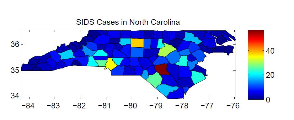
5 Relational Models Tuples recording annual weather conditions at different locations The field-based and object-based approaches are attempts to impose structure and pattern on such data.

6 Object-based Approach Clumps a relation as single or groups of tuples Certain groups of measurements of climatic variables can be grouped together into a finite set of types

7 Object-based Example

8 Field-based approach Treats information as a collection of fields Each field defines the spatial variation of an attribute as a function from the set of locations to an attribute domain

9

10 Object-based Approach

11 Entity Object-based models decompose an information space into objects or entities An entity must be: Identifiable Relevant (be of interest) Describable (have characteristics) The frame of spatial reference is provided by the entities themselves

12 Example: House object Has several attributes, such as registration date, address, owner and boundary, which are themselves objects

13 Spatial objects Spatial objects are called spatial because they exist inside space, called the embedding space A set of primitive objects can be specified, out of which all others in the application domain can be constructed, using an agreed set of operations Point-line-polygon primitives are common in existing systems

14 Example: GIS analysis For Italy s capital city, Rome, calculate the total length of the River Tiber which lies within 2.5 km of the Colosseum First we need to model the relevant parts of Rome as objects Operation length will act on arc, and intersect will apply to form the piece of the arc in common with the disc

15 Example: GIS analysis A process of discretization must convert the objects to types that are computationally tractable A circle may be represented as a discrete polygonal area, arcs by chains of line segments, and points may be embedded in some discrete space

16 Primitive Objects Euclidean Space: coordinatized model of space Transforms spatial properties into properties of tuples of real numbers Coordinate frame consists of a fixed, distinguished point (origin) and a pair of orthogonal lines (axes), intersecting in the origin Point objects Line objects Polygonal objects

17 Points A point in the Cartesian plane R 2 is associated with a unique pair of real number a = (x,y) measuring distance from the origin in the x and y directions. It is sometimes convenient to think of the point a as a vector. Scalar: Addition, subtraction, and multiplication, e.g., (x 1, y 1 ) (x 2, y 2 ) = (x 1 x 2, y 1 y 2 ) Norm: Distance: ab = a-b Angle between vectors:

18 Lines The line incident with a and b is defined as the point set { a + (1 )b R} The line segment between a and b is defined as the point set { a + (1 )b [0, 1]} The half line radiating from b and passing through a is defined as the point set { a + (1 )b 0}

19 Polygonal objects A polyline in R 2 is a finite set of line segments (called edges) such that each edge end-point is shared by exactly two edges, except possibly for two points, called the extremes of the polyline. If no two edges intersect at any place other than possibly at their end-points, the polyline is simple. A polyline is closed if it has no extreme points. A (simple) polygon in R 2 is the area enclosed by a simple closed polyline. This polyline forms the boundary of the polygon. Each end-point of an edge of the polyline is called a vertex of the polygon. A convex polygon has every point intervisible A star-shaped or semi-convex polygon has at least one point that is intervisible

20 Polygonal objects

21 Convexity Visibility between points x, y, and z

22 Example: Triangulation Every simple polygon has a triangulation. Any triangulation of a simple polygon with n vertices consists of exactly n 2 triangles Art Gallery Problem How many cameras are needed to guard a gallery and how should they be placed? Upper bound N/3

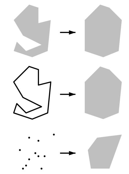
23 Related: Convex Hull

24 Related: Voronoi Diagram

25 Voronoi Diagram on Road Network

26 John Snow, Pumps and Cholera Outbreak

27

28

29 Primitive GIS Operations in Euclidean spaces Length, bearing, area Distance between objects (points, lines, polygons) Centroid Point in polygon Buffer Intersection/overlay In topological spaces Spatial relations (within, touch, cover, )

30 Distance and angle between points Length of a line segment can be computed as the distance between successive pairs of points The bearing,, of q from p is given by the unique solution in the interval [0,360] of the simultaneous equations:

31 Distance from point to line from a point to a line implies minimum distance For a straight line segment, distance computation depends on whether p is in middle(l) or end(l) For a polyline, distance to each line segment must be calculated A polygon calculation is as for polyline (distance to boundary of polygon)

32 Area Let P be a simple polygon (no boundary selfintersections) with vertex vectors: (x 1, y 1 ), (x 2, y 2 ),..., (x n, y n ) where (x 1, y 1 ) = (x n, y n ).Then the area is: In the case of a triangle pqr

33 Area of a simple polygon Note that the area may be positive or negative In fact, area(pqr) = -area(qpr) If p is to the left of qr then the area is positive, if p is to the right of qr then the area is negative

34 Centroid The centroid of a polygon (or center of gravity) of a (simple) polygonal object (P = (x 1, y 1 ), (x 2, y 2 ),..., (x n, y n ) where (x 1, y 1 ) = (x n, y n )) is the point at which it would balance if it were cut out of a sheet of material of uniform density:

35 Point in polygon Determining whether a point is inside a polygon is one of the most fundamental operations in a spatial database Semi-line method (ray casting) : checks for odd or even numbers of intersections of a semi-line with polygon Winding method: sums bearings from point to polygon vertices

36

37 Collinearity and point on segment Boolean operation colinear(a,b,c) determine whether points a, b and c lie on the same straight line Colinear(a,b,c) = true if and only if side (a,b,c) =0 Operation point_on_segment(p,l) returns the Boolean value true if p l (line segment l having end-points q and r) 1 Determine whether p, q, r are collinear 2 If yes, thenp l if and only if p (minimum bounding box) MMB (l)

38 Segment intersection Two line segments ab and cd can only intersect if a and b are on opposite sides of cd and c and d are on opposite sides of ab Therefore two line segments intersect if the following inequalities hold

39 Point of intersection Intersecting line segments l and l in parametric form: Means that there exists an and such that: Which solving for and give:

40 Primitive GIS operations: Intersection, union and overlay of polygons

41 Buffer

42 Topological spatial operations Object types with an assumed underlying topology are point, arc, loop and area Operations: boundary, interior, closure and connected are defined in the usual manner components returns the set of maximal connected components of an area extremes acts on each object of type arc and returns the pair of points of the arc that constitute its end points is within provides a relationship between a point and a simple loop, returning true if the point is enclosed by the loop

43 Topological spatial operations for areas X meets Y if X and Y touch externally in a common portion of their boundaries X overlaps Y if X and Y impinge into each other s interiors

44 Topological spatial operations for areas X is inside Y if X is a subset of Y and X, Y do not share a common portion of boundary X covers Y if Y is a subset of X and X, Y touch externally in a common portion of their boundaries

45 Topological spatial operations There are an infinite number of possible topological relationships that are available between objects of type cell

46 Spaghetti Spaghetti data structure represents a planar configuration of points, arcs, and areas Geometry is represented as a set of lists of straight-line segments

47 Spaghetti- example Each polygonal area is represented by its boundary loop Each loop is discretized as a closed polyline Each polyline is represented as a list of points A:[1,2,3,4,21,22,23,26,27,28,20,19,18,17] B:[4,5,6,7,8,25,24,23,22,21] C:[8,9,10,11,12,13,29,28,27,26,23,24,25] D:[17,18,19,20,28,29,13,14,15,16]

48 Issues There is NO explicit representation of the topological interrelationships of the configuration, such as adjacency Data consistence issues Silver polygons Data redundancy

49 NAA: node arc area Each directed arc has exactly one start and one end node. Each node must be the start node or end node (maybe both) of at least one directed arc. Each area is bounded by one or more directed arcs. Directed arcs may intersect only at their end nodes. Each directed arc has exactly one area on its right and one area on its left. Each area must be the left area or right area (maybe both) of at least one directed arc.

50 NAA: planar decomposition Arc Begin End Left Right a 1 2 A X b 4 1 B X c 3 4 C X d 2 3 D X e 5 1 A B f 4 5 C B g 6 2 D A h 5 6 C A i 3 6 D C

51 Announcement Sammy will not long be our TA, she switches to another research position

52 Finding What s Inside Involves relationship between two or more layers Toxic gas Population Ancient Forest Watersheds

53

54 Overlay: Finding What s Inside What counties are within 50 miles of Interstate 10?

55 Spatial Index Efficient spatial query for massive datasets, e.g., spatial grid index, quadtree, R-tree,.. An example of quadtree

56 Field-based Approach

57 Spatial fields If the spatial framework is a Euclidean plane and the attribute domain is a subset of the set of real numbers; The Euclidean plane plays the role of the horizontal xy-plane The spatial field values give the z-coordinates, or heights above the plane Regional Climate Variations Imagine placing a square grid over a region and measuring aspects of the climate at each node of the grid. Different fields would then associate locations with values from each of the measured attribute domains.

58 Properties of the attribute domain The attribute domain may contain values which are commonly classified into four levels of measurement Nominal attribute: simple labels; qualitative; cannot be ordered; and arithmetic operators are not permissible Ordinal attribute: ordered labels; qualitative; and cannot be subjected to arithmetic operators, apart from ordering Interval attributes: quantities on a scale without any fixed point; can be compared for size, with the magnitude of the difference being meaningful; the ratio of two interval attributes values is not meaningful Ratio attributes: quantities on a scale with respect to a fixed point; can support a wide range of arithmetical operations, including addition, subtraction, multiplication, and division

59 Continuous and differentiable fields Continuous field: small changes in location leads to small changes in the corresponding attribute value Differentiable field: rate of change (slope) is defined everywhere Spatial framework and attribute domain must be continuous for both these types of fields Every differentiable field must also be continuous, but not every continuous field is differentiable

60 One dimensional examples Fields may be plotted as a graph of attribute value against spatial framework Continuous and differentiable; the slope of the curve can be defined at every point

61 One dimensional examples The field is continuous (the graph is connected) but not everywhere differentiable. There is an ambiguity in the slope, with two choices at the articulation point between the two straight line segments. Continuous and not differentiable; the slope of the curve cannot be defined at one or more points

62 One dimensional examples The graph is not connected and so the field in not continuous and not differentiable. Not continuous and not differentiable

63 Two dimensional examples The slope is dependent on the particular location and on the bearing at that location

64 Isotropic fields A field whose properties are independent of direction is called an isotropic field Consider travel time in a spatial framework The time from X to any point Y is dependent only upon the distance between X and Y and independent of the bearing of Y from X

65 Anisotropic fields A field whose properties are dependent on direction is called an anisotropic field. Suppose there is a high speed link AB For points near B it would be better, if traveling from X, to travel to A, take the link, and continue on from B to the destination The direction to the destination is important

66 Spatial autocorrelation Spatial autocorrelation is a quantitative expression of Tobler s first law of geography (1970) Everything is related to everything else, but near things are more related than distant thing Spatial autocorrelation measures the degree of clustering of values in a spatial field Also termed as spatial dependency, spatial pattern, spatial context, spatial similarity, spatial dissimilarity

67 Autocorrelation If like values tend to cluster together, then the field exhibits high positive spatial autocorrelation If there is no apparent relationship between attribute value and location then there is zero spatial autocorrelation If like values tend to be located away from each other, then there is negative spatial autocorrelation

68 Representations of Spatial Fields Points Contours Raster/Lattice Triangulation (Delaunay Trangulation)

69 Example Contour lines and raster

70 Trangulations Example

71 Side Note: Delaunay Triangulation and Dual Graph Voronoi Diagram

72 Operations on fields A field operation takes as input one or more fields and returns a resultant field The system of possible operations on fields in a field-based model is referred to as map algebra Three main classes of operations Local Focal Zonal

73 Neighborhood function Given a spatial framework F, a neighborhood function n is a function that associates with each location x a set of locations that are near to x

74 Local operations Local operation: acts upon one or more spatial fields to produce a new field The value of the new field at any location is dependent on the values of the input field function at that location is any binary operation

75 Focal operations Focal operation: the attribute value derived at a location x may depend on the attributes of the input spatial field functions at x and the attributes of these functions in the neighborhood n(x) of x

76 Zonal operations Zonal operation: aggregates values of a field over a set of zones (arising in general from another field function) in the spatial framework For each location x: 1 Find the Zone Z i in which x is contained 2 Compute the values of the field function f applied to each point in Z i 3 Derive a single value ζ(x) of the new field from the values computed in step 2

77 Summary: Object-based vs Field-based models Object-based models: Greater precision Less redundant information (smaller storage footprints) Complex data structures Field-based models: Simpler data structures More redundant information (larger storage footprints) Less precision Raster is faster, but vector is corrector

78 End of this topic