MAT 102 Introduction to Statistics Chapter 6. Chapter 6 Continuous Probability Distributions and the Normal Distribution

Transcription

1 MAT 102 Introduction to Statistics Chapter 6 Chapter 6 Continuous Probability Distributions and the Normal Distribution 6.2 Continuous Probability Distributions Characteristics of a Continuous Probability Distribution 1. The probability that the continuous random variable X will assume a value between two possible values, X = a and X = b of the variable is equal to the area under the density curve between the values X = a and X = b. 2. The total area (or probability) under the density curve is equal to The probability that the continuous random variable X will assume a value between any two possible values X = a and X = b of the variable is between 0 and 1. Probability Statements Associated with a Continuous Probability Distribution 1. The probability of obtaining a specific value X = a of a continuous variable is zero. That is, P(X = a) = The probability that a continuous variable X assumes a value between a and b, written P(a < X < b), and the probability that a continuous variable X assumes a value from a to b, written P(a X b), are equal. That is, P(a < X < b) = P(a X b). 6.3 The Normal Distribution A normal distribution is a distribution that represents the values of a continuous variable. The importance of a normal distribution is that it serves as a good model in approximating many distributions of real-world phenomena. If a continuous variable is said to be approximately normal, then the normal distribution can be used to model the continuous variable. The graph of a normal distribution is called a normal curve which is a smooth symmetric bell-shaped curve with a single peak at the center. Examples of distributions that can be modeled or approximated by the normal distribution include IQ scores of individuals, adult weights, blood pressure of men and women, tire wear, the size of red blood cells, and the time required to get to work. 6.4 Properties of a Normal Distribution 1. The normal curve is bell-shaped and has a single peak which is located at the center. 2. The mean, median, and mode all have the same numerical value and are located at the center of the distribution. 3. The normal curve is symmetric about the mean. 4. The data values in the normal distribution are clustered about the mean. 5. In theory, the normal curve extends infinitely in both directions, always getting closer to the horizontal axis but never touching it. As the normal curve extends out away from the mean and gets closer to the horizontal axis, the area in the tails of the normal curve is getting closer to zero. 6. The total area under the normal curve is 1 which can also be interpreted as probability. Thus, the area under the normal curve represents 100% of all the data values. 1

2 The Standard Normal Curve For each continuous variable that can be approximated by a normal distribution with a particular mean and standard deviation, there is a normal curve having the same mean and standard deviation which serves as a model of this variable. Consequently, there is no single normal curve, but rather many normal curves which are referred to as a family of curves. Within this family of normal curves, there is only one normal distribution or curve for each combination of mean and standard deviation and the number of possible normal curves is infinite. The proportion of area under any normal curve between the mean and the data value which is N standard deviations away from the mean is the same for all normal curves. Consequently, when working with normal distribution applications it is possible only to have to work with one normal curve since each member of the family of normal distributions exhibits the same characteristics. Although there are an infinite number of normal curves, there is one special member of the normal distribution family that can be used to serve as the normal distribution model for any application. This special normal distribution is referred to as the standard normal distribution. The standard normal distribution has a mean equal to zero, μ = 0, and a standard deviation equal to one, σ = 1. To utilize this standard normal distribution as a model for any normal distribution, it becomes necessary to convert any normal distribution to the standard normal distribution. This is accomplished by converting the values of the continuous variable to z scores. The z score formula helps to convert any normal distribution to the standard x normal distribution. The z score of a data value of x is equal to. Regardless of the values and units of any normal continuous variable, the z score formula can be used to transform any normal distribution to the standard normal distribution with a mean of 0 and a standard deviation of 1. Since any normal distribution can be converted to the standard normal distribution, we only need to refer to one statistical table to find the area under any normal curve rather than an infinite number of tables for all the possible normal curves. This table is called the Standard Normal Curve Area Table. 6.5 Using the Normal Curve Area Table Procedure to Determine the Proportion of Area Under a Normal Curve to the Left of a z Score in Table II 1. Determine which page of Table II to use. 2. Find the row corresponding to the z score under the column labeled z. This row is determined by looking for the integer value and the value of the first decimal place of the z score. 3. Locate the column corresponding to the z score. To determine this column, look for the value of the second decimal place of the z score by moving across the top row of the table until you find the column pertaining to the second decimal place. 4. The entry found in the table where the row and the column determined in steps 2 and 3 intersect represents the proportion of the area to the left of the z score. 2

3 Procedure to Find the Proportion of Area to the Left of a z Score Proportion of area to the left of z = Entry in Table II corresponding to z. Procedure to Find the Proportion of Area to the Right of a z Score 1 Proportion of area to the left of z = Proportion of area to the right of z. Procedure to Find the Proportion of Area Between Two z Scores Proportion of area = Proportion of area to the left of larger z score minus Proportion between two z scores of area to the left of the smaller z score Proportion of Area Associated to a Single z Score Proportion of area for a particular z score equals zero. Example 6.1 pg Find the proportion of area under the normal curve: a) To the left of z = 0.53 (or Less than a z score of 0.53) Using TABLE II: Entry in table for z = 0.53 is which represents the proportion of area to the left of z = nd DISTR 2: normalcdf ( EE99, z score ) ENTER normalcdf ( E99, 0.53) = 0.53 b) To the left of z = 2.56 (or Less than a z score of 2.56) Using TABLE II: Entry in table for z = 2.56 is which represents the proportion of area to the left of z = nd DISTR 2: normalcdf ( EE99, z score ) ENTER normalcdf ( E99, 2.56) = Example 6.2 pg Find the proportion of area under the normal curve: a) To the right of z = 1.37 (or greater than a z score of 1.37) Using TABLE II: Entry in table for z = 1.37 is which represents the proportion of area to the left so Proportion of area to the right of z: 1 Proportion of area to the left of z Proportion of area to the right of z = 1.37 is = nd DISTR 2: normalcdf ( z score, 2 nd EE99 ) ENTER normalcdf ( 1.37, E99) =

4 b) To the right of z = 0.67 (or greater than a z score of 0.67) Using TABLE II: Entry in table for z = 0.67 is which represents the proportion of area to the left so Proportion of area to the right of z: 1 Proportion of area to the left of z Proportion of area to the right of z = 0.67 is = nd DISTR 2: normalcdf ( z score, 2 nd EE99 ) ENTER normalcdf (0.67, E99) = Example 6.3 pg Find the proportion of area under the normal curve: a) Between z = 0 and z = 1.5 Using TABLE II: Entry in table for z = 0 is which represents the proportion of area to the left of z = 0 Entry in table for z = 1.5 is which represents the proportion of area to the left of z = 1.5 Proportion between two z scores: Proportion of area to the left of larger z score of area to the left of the smaller z score Proportion of area between z = 0 and z = 1.5 is = nd DISTR 2: normalcdf ( smaller z score, larger z score ) ENTER normalcdf (0, 1.5) = c) Between z = 1.25 and z = 1.0 Using TABLE II: Entry in table for z = 1.25 is which represents the proportion of area to the left of z = 1.25 Entry in table for z = 1.0 is which represents the proportion of area to the left of z = 1.0 Proportion between two z scores: Proportion of area to the left of larger z score of area to the left of the smaller z score Proportion of area between z = 1.25 and z = 1.0 is = normalcdf ( 1.25, 1.0) =

5 Example 6.5 pg For a normal distribution, find the z score(s) that cut(s) off: a) The lowest 20% of area. (or cuts off the bottom 20 % or 0.20 of the z scores) Lowest 20% = lower proportion of area is 0.20 which is to the left of the mean = 0 so we can use TABLE II to find the z score with the proportion of area to the left closest to 0.20 Entry in table for z = 0.84 is Thus the z score which cuts off the lowest 20% of area in a normal distribution is z = 0.84 invnorm (0.20) = 0.84 b) The highest of 10% of area (or cuts off the top 10 % or 0.10 of the z scores) Highest 10% = 0.10 in decimal form which is to the right of the mean = 0 and is the upper 0.10 proportion of area so we must change this to the left of a z score in order to use the table: Proportion of area to the left of a z score = 1 proportion of area to the right = = 0.90 Use TABLE II to find the z score with the proportion of area to the left closest to 0.90 Entry in table for z = 1.28 is Thus the z score which cuts off the highest 10% of area in a normal distribution is z = 1.28 invnorm (0.90) = 1.28 c) The middle 90% of the area (or of the z scores) In a normal distribution, z = 0 is located in the center so middle 90% represents 45% to the left of z = 0 and 45% to the right of z = 0. Since the proportion of area to the left of z = 0 is 50% or 0.50 then the remaining proportion of area to the left of the smaller z value is = 0.05 Use TABLE II to locate the area which is closest to the proportion of area of 0.05 and determine the z score for this area. Thus the z scores which cuts off the middle 90% of the normal distribution are z = 1.65 and z = 1.65 invnorm (0.05) = 1.64 since there will also be another z-score which is the same but opposite sign you have z =

6 6.6 Applications of the Normal Distribution Example 6.6 pg. 316 Assume the distribution of tire wear is approximately normal with: = 48,000; = 2,000. Find the proportion of tires which would be expected to wear: a) Less than 46,000 miles b) Greater than 49,000 miles c) Between 47,000 and 51,000 miles a) Less than 46,000 miles z Use the TI-83/84 normalcdf 2 nd DISTR 2 lowest data value, highest data value,, ENTER normalcdf ( E99, 46000, 48000, 2000) = ANS: The the proportion of tires that is expected to wear less than 46,000 miles is.1587 b) Greater than 49,000 miles normalcdf (49000, E99, 48000, 2000) ANS: The proportion of tires that is expected to wear more than 49,000 is

7 c) Between 47,000 and 51,000 miles normalcdf (47000, 51000, 48000, 2000) = ANS: The proportion of tires that is expected to wear between 47,000 and 51,000 is.6247 Note: If asked for the percent of tires which would be expected to wear 47,000 and 51,000 the answer would be 62.47% Example 6.7 pg. 317 A distribution of IQ scores is normally distributed with a mean of 100 and a standard deviation of 15. Find the proportion of IQ scores that are: c) Less than 70 or greater than 145. = 100; = 15 Since we are looking for the areas around the tails, we need to find the proportion of area between 70 and 145 and subtract that from 1 normalcdf (70, 145, 100, 15) = so = ANS: The proportion of IO scores less than 70 and greater than 145 is.0241 Example 6.8 pg. 319 One thousand students took a standardized psychology exam. The results were approximately normal with = 83 and = 8. Find the number of students who scored: a) Less than 67 normalcdf ( E 99, 67, 83, 8) = To find the number of students and not the proportion of area we must multiply the proportion with the total number of students that took the test. (0.0228) (1000) = 22.8 or 23 students scored less than 67 7

8 6.7 Percentiles and Applications of Percentiles Percentiles are widely used to describe the position of a data value within a distribution. The percentile rank of a data value X within a normal distribution is equal to the percent of area under the normal curve to the left of the data value X. Percentile ranks are always expressed as a whole number. Procedure to Find Data Value (or Raw Score) that Cuts off Bottom p% Within a Normal Distribution 1. Change the percentage p to a proportion. 2. Using Table II, find the z score that has the area closest to this proportion. If there is a tie, choose the z score with the larger absolute value. 3. Substitute this z score into the raw score formula X = μ + (z)σ to determine the data value that corresponds to this z score. Procedure to Find Data Value (or Raw Score) that Cuts off Top q% Within a Normal Distribution 1. Calculate the percentage of data values below the raw score by subtracting q from 100: (100 q). 2. Change this percentage to a proportion. 3. Using Table II, find the z score that has the area closest to this proportion. If there is a tie, choose the z score with the larger absolute value. 4. Substitute this z score into the raw score formula X = μ + (z)σ to determine the data value that corresponds to this z score. Example 6.9 pg. 320 Matthew earned a grade of 87 on his history exam. If the grade in his class were normally distributed with = 80 and = 7, find Matthew s percentile rank on this exam. normalcdf ( E 99, 87, 80, 7) = (proportion of area to the left) (100) = 84.13% Percentile Rank = 84 Notation for this is: 87 = P 84 8

9 Example 6.10 pg. 321 Miss Brooks took two exams. Her grades and the class results are as follows: Student Class Class Standard Exam Grade mean () Deviation () English Math Use percentile ranks to determine on which test(s) the student did better relative to her class For English: normalcdf ( E 99, 83, 80, 6) = = 69.15% = percentile rank is 69 ANS: The percentile rank of the student s English grade of 83 is 69, expressed as P 69 = 83 For Math: normalcdf ( E 99, 77, 74, 5) = = 72.57% = percentile rank is 73 ANS: The percentile rank of the student s Math grade of 77 is 73, expressed as P 73 = 77 Conclusion: The percentile rank of the student s math grade is greater than the percentile rank of her English grade Relative to her class, the student did better on her math exam 9

10 Example 6.10 pg. 321 Assume the distribution of the playing careers of major league baseball players can be approximated by a normal distribution with a mean of 8 years and a standard deviation of 4 years. Find the probability that a player selected at random will have a career that will last: a) Less than 6 years b) Longer than 14 years c) Between 4 and 10 years 10

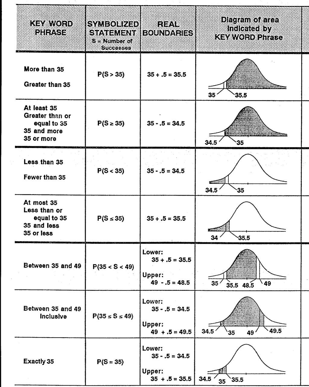
11 6.9 The Normal Approximation to the Binomial Distribution Definitions n = p = number of trials the probability of success in one trial 1 p = the probability of failure in one trial s = mu sub s = s np sigma sub s = np( 1 p) s Required calculations for the Normal Approximation to the Binomial Distribution Conditions of Normal Approximation of a Binomial Distribution You can use the approximation by a normal distribution, with a mean of s and a s when both: np and n(1 p) each >5 Example 6.20 p.341 Consider the binomial experiment of tossing a fair coin 100 times. Use the normal approximation to calculate the probability of getting: a) At least 55 heads b) Between 40 and 60 heads c) Exactly 54 heads d) At most 45 heads n = 100 p = ½ n = 1 - ½ = ½ np 100 (.5) 50 s s np(1 p) a) Probability of getting at least 55 heads np and n(1 p) each >5 so we can use normal Let x = 54.5, which is the lower boundary of 55 and the correction for continuity We are looking for the area under the curve that is to the right of normalcdf ( lower value, upper value, s, s) normalcdf ( 54.5, E99, 50, 5) = So the probability of getting at least 55 heads is approximately

12 b) Probability of getting between 40 and 60 heads (not inclusive) Use the upper boundary of 40, which is 40.5 and the lower boundary of 60, which is 59.5 normalcdf ( 40.5, 59.5, 50, 5) = c) Probability of getting exactly 54 heads normalcdf (53.5, 54.5, 50, 5) = d) Probability of getting at most 45 heads This is the same as saying getting 45 heads Use x = 45.5, which is the upper boundary of 45 normalcdf ( E99, 45.5, 50, 5) = See Examples 6.21 & 6.22 pg

13 13