image filtration i Ole-Johan Skrede INF Digital Image Processing

Transcription

1 image filtration i Ole-Johan Skrede INF Digital Image Processing Department of Informatics The Faculty of Mathematics and Natural Sciences University of Oslo After original slides by Fritz Albregtsen

2 messages The first mandatory assignment: Tentative posting date: Wednesday Tentative submission deadline: Friday

3 today s lecture Neighbourhood operations Convolution and correlation Low pass filtering Sections in Gonzales & Woods: 2.6.2: Linear versus Nonlinear Operations 3.1: Background 3.4: Fundamentals of Spatial Filtering 3.5: Smoothing spatial Filtering 5.3: Restoration in the Presence of Noise Only Spatial Filtering : Matching by correlation 2

4 image filtering

5 overview A general tool for processing digital images. One of the mostly used operations in image processing. Typical utilities: Image improvement Image analysis Remove or reduce noise Improve percieved sharpness Highlight edges Highlight texture 4

6 spatial filtering The filter (or filter kernel) is defined by a matrix, e.g. w = w[ 1, 1] w[ 1, 0] w[ 1, 1] w[0, 1] w[0, 0] w[0, 1] w[1, 1] w[1, 0] w[1, 1] Filter kernels are often square with odd side lenghts. In this lecture, we will always assume odd side lengths unless otherwise is specified. As with images, we index the filter as w[x, y], where the positive x axis is downward and the positive y axis is to the right. The origin of the filter is at the filter center. We use the names filter and filter kernel interchangeably. Other names are filter mask and filter matrix. The result of the filtering is determined by the size of the filter and the values in the filter. 5

7 general image filtering Figure 1: Example of an image and a 3 3 filter kernel. 6

8 convolution introduction and example

9 convolution In image analysis 1, convolution is a binary operation, taking an image f and a filter (also an image) w, and producing an image g. We use an asterisk to denote this operation f w = g. For an element [x, y], the operation is defined as S T g[x, y] = (f w)[x, y] := f[x s, y t]w[s, t]. s= S t= T 1 This is really just an ordinary discrete convolution, the discrete version of a continuous convolution. 8

10 convolution Let us walk through a small example, step by step Figure 2: Extract of an image f, a 3 3 filter kernel with values, and a blank result image g. The colored squares indicate which elements will be affected by the convolution. Notice that we are in the interior of the image, this is because boundaries require some extra attention. We will deal with boundary conditions later. 9

11 convolution 1 locations First, our indices (x, y), will be as indicated by the figure, and we will only affect values inside the coloured squares. In this example. S = 1 and T = 1. g[x, y] = (f w)[x, y] := 1 s= 1 t= 1 1 f[x s, y t]w[s, t]. Figure 3: Locations in first convolution. 10

12 convolution 1 step 1: s = 1, t = g[x, y] = f[x s, y t]w[s, t] s= 1 t= 1 g[x, y] = =

13 convolution 1 step 2: s = 1, t = g[x, y] = f[x s, y t]w[s, t] s= 1 t= 1 g[x, y] = =

14 convolution 1 step 3: s = 1, t = g[x, y] = f[x s, y t]w[s, t] s= 1 t= 1 g[x, y] = =

15 convolution 1 step 4: s = 0, t = g[x, y] = f[x s, y t]w[s, t] s= 1 t= 1 g[x, y] = =

16 convolution 1 step 5: s = 0, t = g[x, y] = f[x s, y t]w[s, t] s= 1 t= 1 g[x, y] = =

17 convolution 1 step 6: s = 0, t = g[x, y] = f[x s, y t]w[s, t] s= 1 t= 1 g[x, y] = =

18 convolution 1 step 7: s = 1, t = g[x, y] = f[x s, y t]w[s, t] s= 1 t= 1 g[x, y] = =

19 convolution 1 step 8: s = 1, t = g[x, y] = f[x s, y t]w[s, t] s= 1 t= 1 g[x, y] = =

20 convolution 1 step 9: s = 1, t = g[x, y] = f[x s, y t]w[s, t] s= 1 t= 1 g[x, y] = =

21 convolution 2 step 1: s = 1, t = g[x, y] = f[x s, y t]w[s, t] s= 1 t= 1 g[x, y] = =

22 convolution 2 step 9: s = 1, t = g[x, y] = f[x s, y t]w[s, t] s= 1 t= 1 g[x, y] = =

23 convolution 3 step 9: s = 1, t = g[x, y] = f[x s, y t]w[s, t] s= 1 t= 1 g[x, y] = =

24 convolution 4 step 9: s = 1, t = g[x, y] = f[x s, y t]w[s, t] s= 1 t= 1 g[x, y] = =

25 useful mental image A useful way of thinking about convolution is to 1. Rotate the filter 180 degrees. 2. Place it on top of the image in the image s top left corner. 3. Slide it across each column until you hit the top right corner. 4. Start from the left again, but now, one row below the previous. 5. Repeat step 3. followed by 4. until you have covered the whole image. Also, check out this nice interactive visualization: 24

26 boundary treatment

27 different modes We differentiate between three different modes when we filter one image with another: Full: We get an output response at every point of overlap between the image and the filter. Same: The origin of the filter is always inside the image, and we pad the image in order to preserve the image size in the result. Valid: We only record a response as long as there is full overlap between the image and the whole filter. 26

28 full mode This can be written as as long as (f w)[x, y] = f[x s, y t]w[s, t] s= t= (x s) is a row in f and s is a row in w (1) for some s, and (y t) is a column in f and t is a column in w (2) for some t. 27

29 full mode size If f is of size 1 M N and w of size P Q, assuming M P and N Q, the output image will be of size M + P 1 N + Q 1. That is, Number of rows: M + P 1. Number of columns: N + Q 1. 1 We use the rows columns convention when describing the size of an image. 28

30 full mode example full =

31 valid mode This can be written as as long as (f w)[x, y] = f[x s, y t]w[s, t] s= t= (x s) is a row in f and s is a row in w (3) for all s, and (y t) is a column in f and t is a column in w (4) for all t. 30

32 valid mode size If f is of size M N and w of size P Q, assuming M P and N Q, the output image will be of size M P + 1 N Q + 1. That is Number of rows: M P + 1. Number of columns: N Q

33 valid mode example valid = [ ] 32

34 same mode This is the same as valid mode, except that we pad the input image (add values outside the original boundary) such that the output size is the same as the original image. We will cover three types of paddings, and use a 1D example to illustrate. In the 1D example, we assume an original signal of length 5, and we pad with 2 on each side, furthermore we use to indicate the original boundary. Zero padding [0, 0 1, 2, 3, 4, 5 0, 0] Symmetrical padding [2, 1 1, 2, 3, 4, 5 5, 4] Circular padding [4, 5 1, 2, 3, 4, 5 1, 2] 33

35 same mode size For a filter with size P Q, we must pad the image with P 1 2 rows on each side, and Q 1 2 columns on each side. We can check that this will produce an output of size M N by calculating the output side from the valid mode: [ ] P 1 M + 2 P + 1 = M 2 [ ] Q 1 N + 2 Q + 1 = N 2 (5) 34

36 same mode zero padding Can also pad with other constant values than same zero =

37 same mode symmetric padding Also known as mirrored padding or reflective padding same symmetric =

38 same mode circular padding Also known as wrapping same circular =

39 properties, general case Commutative Associative Distributive (f w)[x, y] = Associative with scalar multiplication = S T s= S t= T x+s y+t s=x S t=y T f[x s, y t]w[s, t] f[s, t]w[x s, y t] f g = g f (f g) h = f (f h) f (g + h) = f g + f h α(f g) = (αf) g = f (αg) 38

40 correlation and template matching

41 correlation In this case, correlation is a binary operation, taking an image f and a filter (also an image) w, and producing an image g. For an element [x, y], the operation is defined as g[x, y] = (f w)[x, y] := S T s= S t= T f[x + s, y + t]w[s, t]. Very similar to convolution. Equivalent if the filter is symmetric. For the mental image, it is the same as convolution, without the rotation of the kernel in the beginning. In general not associative, which is important in some cases. Less important in other cases, such as template matching. 40

42 template matching We can use correlation to match patterns in an image. Remember to normalize the image and the filter with their respective means. 41

43 template matching example You can find an example implementation in python at (separable_timing.ipynb). 42

44 neighbourhood operators

45 filtering in the image domain In general, we can view filtering as the application of an operator that computes the result image s value in each pixel (x, y) by utilizing the pixels in the input image in a neighbourhood around (x, y) g[x, y] = T (f[n (x, y)]) In the above, we assume that g[x, y] is the value of g at location (x, y) and f[n (x, y)] is the value(s) in the neighbourhood N (x, y) of (x, y). T is some operator acting on the pixel values in the neighbourhood. 44

46 neighbourhood The neighbourhood of the filter gives the pixels around (x, y) in the input image that the operator (potentially) use. Figure 6: Neighbourhood example, a 5 5 neighbourhood centered at (x, y), and a 3 3 neighbourhood centered at (x + 4, y + 5). 45

47 neighbourhood in practice Squares and rectangles are most common. For symmetry reasons, the height and width is often odd, making the location of the center point at a pixel. When nothing else is specified, the origin of the neighbourhood is at the center pixel. If the neighbourhood is of size 1 1, T is grayscale transform. If T is equal over the whole image, we say that T is a global operator. If the neighbourhood size is greater than 1 1, we term T as a local operator (even if T is position invariant). 46

48 neighbourhood + operator = filter Neighbourhood Define the set of pixels around (x, y) in the input image where T operates. Operator Filter Defines the operation done on the values in the pixels in the neighbourhood. Also called a transform or an algorithm. A filter is an operator operating on a neighbourhood, that is, two filters are equivalent only if both the neighbourhood and the operator are equal. 47

49 additivity A filter is said to be additive if T ((f 1 + f 2 )[N (x, y)]) = T (f 1 [N (x, y)]) + T (f 2 [N (x, y)]) where T is the operator. N (x, y) is the neighbourhood around an arbitrary pixel (x, y). f 1 and f 2 are arbitrary images. 48

50 homogeneity A filter is said to be homogeneous if T (αf[n (x, y)]) = αt (f[n (x, y)]) where T is the operator. N (x, y) is the neighbourhood around an arbitrary pixel (x, y). f is an arbitrary image. α is an arbitrary scalar value. 49

51 linearity A filter is said to be linear if it is both additive and homogeneous, that is, if T ((αf 1 + βf 2 )[N (x, y)]) = αt (f 1 [N (x, y)]) + βt (f 2 [N (x, y)]) where T is the operator. N (x, y) is the neighbourhood around an arbitrary pixel (x, y). f 1 and f 2 are arbitrary images. α and β are arbitrary scalar values. 50

52 position invariance A filter is said to be position invariant if where T is the operator. T (f[n (x s, y t)]) = g(x s, y t) N (x, y) is the neighbourhood around an arbitrary pixel (x, y). f 1 and f 2 are arbitrary images. g(x, y) = T (f[n (x, y)]) for all (x, y). (s, t) is an arbitrary position shift. In other words, the value of the result image at (x, y) is only dependent of the values in the neighbourhood of (x, y), and not dependent on the positions. 51

53 separable filters A 2D filter w, is said to be separable if the filtration can be done with two sequential 1D filtrations, w V and w H. In other words, if w = w V w H An example is a 5 5 mean filter [ ] =

54 separable filters are faster From the associativity of convolution, with f as an image and w = w V w H, we get f w = f (w V w H ) = (f w V ) w H As can be seen, we can now do two convolutions with a 1D filter, in stead of one convolution with a 2D filter, that is g = f w, vs. h = f w V g = h w H 2D 1D 1D 53

55 implementation Illustrative (ignores padding etc.) examples of implementations, where f, input image, size [M, N] w, 2D filter kernel, size [L, L], (S = T = (L - 1) / 2) w_v, w_h, vertical filter kernels, size [L] h, temporary filtered image, size [M, N] g, filtered image, size [M, N] 1 # Convolution with 2D f i l t e r 2 for x in range (M) : 3 for y in range (N) : 4 for s in range( S, S ) : 5 for t in range( T, T ) : 6 g [ x, y ] = f [ x s, y t ] *w[ s, t ] 7 1 # Convolution with 2 1D f i l t e r s 2 for x in range (M) : 3 for y in range (N) : 4 for s in range( S, S ) : 5 h [ x, y ] = f [ x s, y ] * w_v [ s ] 6 for x in range (M) : 7 for y in range (N) : 8 for t in range( T, T ) : 9 g [ x, y ] = h [ x, y t ] * w_h[ t ] 10 54

56 how much faster? complexity For an M N image and a square filter kernel with sidelengths L, a (naive) 2D convolution implementation would have complexity of O(MNL 2 ), while a (naive) 1D convolution implementation would have complexity of So the speed up should be linear in L. O(MNL). 55

57 flops Looking back at our naive implementations, we see that in the case of the 2D filter, we have about MNL 2 multiplications and MN(L 2 1) additions, so about flops nonsep = MNL 2 + MN(L 2 1) = MN(2L 2 1) floating point operations (FLOPS). For the case with 2 1D filters, we have about 2MNL multiplications and 2MN(L 1), which is then flops sep = 2MNL + 2MN(L 1) = 2MN(2L 1). 56

58 how much faster? flops We can get an idea of the speedup by looking at flops nonsep = 2L2 1 flops sep 4L 2 2L So the 2D case should be about L times slower than the separable case. For a concrete example, take a look here: 57

59 intermezzo how did we arrive at the asymptotic speed up I do not like math magic in my slides, so I will now show how 2L 2 1 4L 2 2L We say that they are asymptotically equivalent, and write to symbolise this. This simply means that the one approaches the other as L increases. 2L 2 1 4L 2 = L2 2L 1 1 4L 2 L 2 (2L + 1) = (2L 1)(2L + 1) 1 4L 2 = L 2 1 (2L) 2 (2L + 1) 12 4L 2 L 2 1 = (4L 2 (2L + 1) 1) 4L = (4 1 (2L + 1) L ) 4L 2 2 L 2L

60 convolution with update Convolution filters with identical columns or rows can be implemented efficiently by updating already computed values. 1. Compute the response r x,y at a pixel (x, y). 2. Compute the response in the next pixel from r xy : Identical columns: r x,y+1 = r x,y C 1 + C L, where C 1 is the column response from the first column when the kernel origin is at (x, y), and C L is the column response from the last column when the kernel origin is at (x, y + 1). Identical rows: r x+1,y = r x,y R 1 + R L, where R 1 is the row response from the first row when the kernel origin is at (x, y), and R L is the row response from the last row when the kernel origin is at (x + 1, y). 3. Repeat from 2. 59

61 convolution with update illustration Figure 7: Top: reusing columns; bottom: reusing rows. 60

62 convolution with update speed gain C 1, C L, R 1 and R L can (individually) be computed with L multiplications and L 1 additions. This means that computing the new response requires 2L multiplications and 2L additions. This is as fast as separability. If we ignore the initialization; we must compute one full convolution to restart the updates at every new row or column. All filters that can be updated in this way, is also separable. Conversly, separable filters need not be updatable. Can be combined with separability when a 1D filter is uniform. Uniform filters can be computed even faster. Each update only needs 2 subtractions and 1 addition. Only filters that are proportional to the mean value filter are uniform. 61

63 low-pass filters

64 some common filter categories Low-pass filters Lets through low frequencies, stops high frequencies. Blurs the image. High-pass filters Lets through high frequencies, stops low frequencies. Sharpens the image. Band-pass filters Lets through frequencies in a certain range. Feauture detection filters Used for detection of features in an image. Features such as edges, corners and texture. 63

65 low-pass filter overview Lets through low frequencies (large trends and slow variations in an image). Stops or damps high frequencies (noise, details and sharp edges in an image). We will learn more about frequencies in the lectures about Fourier transforms. The resulting image is a smeared, smoothed or blurred version of the original image. Typical applications: Remove noise, locate larger objects in an image. Challenging to preserve edges. 64

66 mean value filter Computes the mean value in the neighbourhood. All weights (values in the filter) are equal. The sum of the weights is equal to 1. The neighbourhood size determines the blurring magnitude. Large filter: Loss of details, more blurring. Small filter: Preservation of details, less blurring , ,

67 mean value filter example (a) Original (b) 3 3 (c) 9 9 (d) Figure 8: Gray level Mona Lisa image filtered with a mean value filter of different sizes. 66

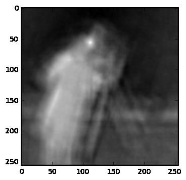
68 mean value filtering locate large objects Objective: Locate large, bright objects. Possible solution: mean value filtering followed by a global thresholding. Figure 9: Left: Image obtained with the Hubble Space Telescope. Middle: Result after mean value filtering. Right: Result after global thresholding of the filtered image. 67

69 gaussian filter For integer valus x, y, let w[x, y] = A exp { x2 + y 2 } 2σ 2 where A is usually such that x y w[x, y] = 1. This is a non-uniform low-pass filter. The parameter σ is the standard deviation and controls the amount of smoothing. Small σ: Less smoothing Large σ: More smoothing A Gaussian filter smooths less than a uniform filter of the same size. (a) σ = 1 (b) σ = 2 Figure 10: Continuous bivariate Gaussian with different σ. Implementation can be found at 68

70 approximation of gaussian filter A 3 3 Gaussian filter can be approximated as w = This is separable as 4 1D filters 1 2 [1, 1]: [ ] w = [ 1 1 [ ] ] 1 2 [ 1 1 [ ] = ] 1 4 [ ]. Or two 1D filters 1 4 [1, 2, 1]: w = [ ]. 69

71 edge-preserving noise filtering We often use low-pass filters to reduce noise, but at the same time, we want to keep edges. There exists a lot of edge-preserving filters. Many works by utilising only a sub-sample of the neighbourhood. This could be implemented by sorting pixels radiometrically (by pixel value), and/or geometrically (by pixel location). In the example from fig. 11, we could choose to only include contributions from within the blue ball. Figure 11: Blue ball on white background. Red square to illustrate filter kernel. 70

72 rank filtering We create a one-dimensional list of all pixel values around (x, y). We then sort this list. Then, we compute the response from (x, y) from one element in the sorted list, or by some weighted sum of the elements. This is a non-uniform filter. 71

73 median filtering A rank filter where we choose the middle value in the sorted list of values in the neighbourhood of (x, y). One of the most frequently used edge-preserving filters. Especially well-suited for reducing impulse-noise (aka. salt-and-pepper-noise ). Not unusual with non-rectangular neighbourhood, e.g. plus-shaped neighbourhoods. Some challenges: Thin lines can dissappear Corners can be rounded Objects can be shrinked The size and shape of the neighbourhood is important 72

74 mean value- and median- filters Figure 12: Left: Image with salt and pepper noise. Middle: Mean value filtering. Right: Median filtering. 73

75 mean value- and median- filters Mean value filter: The mean value inside the neighbourhood. Smooths local variations and noise, but also edges. Especially well suited on local variations, e.g. mild noise in many pixel values. Median value filter: The median value inside the neighbourhood Better for certain types of noise and preserves edges better. Worse on local variations and other kinds of noise. Especially well suited for salt-and-pepper-noise. 74

76 median filters and corners Figure 13: Left: Quadratic neighbourhood rounds corners. Right: pluss-shaped neighbourhood preserves corners. 75

77 faster median filters (cursory reading) Sorting pixel values are slow (general worst case: O(n log(n)), where n is the number of elements (here, n = L 2 )). Using histogram-updating techniques, we can achieve O(L) 1 Utilizing histogram-updating even more, we can achieve O(1) 1 1 Huang, T.S., Yang, G.J., Tang, G.Y.: A Fast Two-Dimensional Median Filtering Algorithm, EEE TASSP 27(1), 13-18, Perreault and Hébert: Median filtering in constant time, IEEE TIP 16(9), ,

78 alpha-trimmed mean value filter The response is computed as the mean value of the P Q d middle values (after sorting) in the P Q neighbourhood around (x, y). Let Ω x,y be the set of pixel positions of the P Q d middle values after sorting, then the response is given by g[x, y] = 1 P Q d For d = 0 this becomes the mean value filter. For d = P Q 1 this becomes the median filter. (s,t) Ω x,y f[s, t]. 77

79 mode filter (cursory reading) The response g[x, y] is equal to the most frequent pixel value in N (x, y). The number of unique pixel values must be small compared to the number of pixels in the neighbourhood. Mostly used on segmented images containing only a few color levels to remove isolated pixels. (a) Segmented image (b) After mode filtering Figure 14: Segmented image before and after mode filtering. 78

80 k-nearest-neighbour filter g[x, y] is the mean value of the K nearest pixel values in N (x, y). Here, nearest is in terms of absolute difference in value. Problem: K is constant for the entire image. Too small K: We remove too little noise. Too large K: We remove edges and corners. How to choose K for a L L neighbourhood, where L = 2S + 1. K = 1 : no effect. K L : preserves thin lines. K (S + 1) 2 : preserves corners. K (S + 1)L : preserves straight lines. 79

81 k-nearest-connected-neighbour filter The neighbourhood N (x, y) is the entire image. Thin lines, corners and edges are preserved if K is smaller or equal the number of pixels in the object. The implementation is something like this 1 # K nearest connected neighbours ( pseudocode ) 2 # f i s o r i g i n a l image, and g i s f i l t e r e d image, both of shape [M, N] 3 for x in range (M) : 4 for y in range (N) : 5 chosen_vals = [ ] 6 chosen_pixel = ( x, y ) 7 candidate_vals = [ ] 8 candidate_ pixels = [ ] 9 while len ( chosen_vals ) <= K : 10 candidate_ pixels. append_unique ( neighbourhood ( chosen_pixel ) ) 11 candidate_vals = f [ candidate_pixels ] 12 chosen_pixel = candidate_ pixels. pop ( argmin ( abs ( candidate_vals f [ x, y ] ) ) ) 13 chosen_vals. append ( f [ chosen_pixel ] ) 14 g [ x, y ] = mean( chosen_vals ) 15 80

82 minimal mean square error (mmse) filter For a P Q neighbourhood N (x, y) of (x, y), we can compute the sample mean µ(x, y) and variance 1 σ 2 (x, y) µ(x, y) = 1 P Q σ 2 (x, y) = 1 P Q = 1 P Q (s,t) N (x,y) (s,t) N (x,y) (s,t) N (x,y) f[s, t] (f[s, t] µ(x, y)) 2 f 2 [s, t] µ 2 (x, y) Assume that we have an estimate of the noise-variance σ 2 η Then, the MMSE-response at (x, y) is given as f[x, y] σ2 η σ g[x, y] = 2 (x,y) (f[x, y] µ(x, y)), σ2 η σ 2 (x, y) µ(x, y), ση 2 > σ 2 (x, y). In homogeneous areas, the response will be close to µ(x, y) Close to edges will σ 2 (x, y) be larger than σ 2 η, resulting in a response closer to f[x, y]. 1 For an unbiased estimator of the variance, the denominator is P Q 1. 81

83 sigma filter (cursory reading) The filter result g[x, y] is equal to the mean value of the pixels in the neighbourhood N (x, y) with values in the interval f[x, y] ± kσ. σ is a standard deviation estimated from homogeneous regions in f. k is a parameter with an appropriate problem-dependent value. S T s= S t= t g[x, y] = w xy[s, t]f[x + s, y + t] S T s= S t= t w, xy[s, t] where { 1, if f[x, y] f[x + s, y + t] kσ w xy [s, t] = 0, if not. 82

84 max-homogeneity filter An edge-preserving filter. Form multiple overlapping sub-neighbourhoods from the original neighbourhood. There exist many different ways to split the neighbourhood. Every sub-neighbourhood should contain the original centre pixel. The most homogeneous (e.g. with smallest variance) sub-neighbourhood contains the least edges. Computation: Compute the mean value and variance in each sub-neighbourhood. Set g[x, y] equal to the mean value of the sub-neighbourhood with lowes variance. 83

85 symmetrical nearest neighbour (snn) filter For every symmetrical pixel-pair in the neighbourhood of (x, y): Choose the pixel with the closest value to f[x, y] g[x, y] is then the mean value of the chosen pixel values and f[x, y]. The number of values that are meaned in a P Q neighbourhood is then (P Q 1)/

86 table of some low-pass filters Most important Mean value filter Gaussian filter Median filter Other examples covered today Alpha-trimmed mean value filter Mode filter K-nearest-neighbour filter K-nearest-connected-neighbour filter MMSE filter Sigma filter Max-homogeneity filter Symmetrical nearest neighbour filter Other examples not covered today Family of image guided adaptive filters (e.g. anisotropic diffusion filter) 85

87 summary Spatial filter: a neighbourhood and an operator. The operator defines the action taken on the input image. The neighbourhood defines which pixels the operator use. Convolution is linear spatial filtering Knowing how this works is essential in this course. Knowing how to implement this is also essential. Correlation can be used for template matching Low-pass filters can reduce noise, and there are many different low-pass filters. 86

88 Questions? 87