Supplemental Quick Guide to GeoWEPP

Transcription

1 Supplemental Quick Guide to GeoWEPP Table of Contents Page A. Rasters needed to run GeoWEPP 1. NED or DEM 2. Topographic Raster B. Before starting the GeoWEPP program 1. Fixing the coordinate system projection error in GeoWEPP 2. Changing the projection of a raster 3. Changing NED to ASCII C. Starting GeoWEPP 1. Changing the Layer projection 2. Add the topographic raster 3. Selecting a watershed D. Selecting the Climate, Management, Soil files 1. Selecting a climate 2. Selecting a soil file 3. Selecting a landuse (management) file 4. Running a model Appendix A Checking the spatial reference of rasters 22 Appendix B Spatial change for Windows 2000 and ArcGIS 9.X 23 Appendix C Downloading a climate file from FSWEPP 29 Appendix D Importing a climate file to WEPP windows 33 Appendix E Quick guide to WEPP windows management calibration 35 Document End 52 Questions? Corrections? suemiller@fs.fed.us

2 Introduction This Quick Guide is not a substitute for the GeoWEPP or GeoWEPPBAER instruction manuals (Specialized GeoWEPP Interface for Burned Area Emergency Response Teams Manual and GeoWEPP for ArcGIS 9.x Full Version Manual). The author recommends reading the manuals and using the example data provided before attempting to use the GeoWEPP program with your own data. In this way, you will have a general idea of what is supposed to happen when running a simulation with this program. With that being said, chances are you can not run your own data without some pre-processing in either program. This Quick Guide provides instruction for the GeoWEPP program. All data used in the proceedings examples are from an example used at the Ogden workshop in 2008 Mt Charleston outside of Las Vegas, NV. Something you may wish to do, but is not necessary, is to build your own management files. You may choose a file that is already calibrated (outlined in section D. Selecting the Management and Soil Files) or calibrate a management file yourself. Appendix E. A. Rasters needed to run GeoWEPP (Return) Two rasters are needed to run GeoWEPP; 1) NED or DEM and 2) a topographic raster. You can acquire both the NED and topographic map at the same site. 1. NED or DEM On this site you will need your eauthentication user name and password to view and retrieve the extended options offered. If you are not a forest service employee, eauthentication user names and passwords can be acquired from your local Natural Resources Conservation Service (NRCS) office. When you find the location of your project and select the area, a screen will give you several options. Choose a 10 or 30 meter NED. You may (but not always) have trouble running the model with a 10-meter NED because of size/memory compatibility issues. I generally use a 30-meter NED. 2. Topographic Raster - Topographic rasters can be retrieved from the same site as the NED. Choose the NED and Digital Raster Graphics (DRG) and continue through the steps (figure below). When you are finished with this process, the datagateway will send you a link via to download the rasters. 2

3 Once the items are downloaded, copy the folder to a working directory within the GeoWEPP folder program structure. Placing a copy of the rasters within the GeoWEPP directory will make life simple in case of errors when processing data, plus it will save time navigating through the file structure. B. Before starting the GeoWEPP program (Return) 1. Fixing the coordinate system projection error in GeoWEPP a. Navigate to the location of the Required Files folder in GeoWEPP on your C drive. C:\GeoWEPP\Required_Files. Open the ArcGeoWEPP.mxd file in this folder. 3

4 b. Once ArcMap displays, right click the Layer data frame in the TOC > select properties. c. Select the Coordinate System tab. Notice that the projection listed is NAD 1927_UTM_Zone_13N. 4

5 d. Select the Clear button at the top right hand corner of this tab. Click apply and OK. e. Save and close the mxd. 2. Changing the projection of a raster The raster you wish to project must be in its original form. This step is the best method for lining up the fire severity raster with the channel network in GeoWEPP. You can not use a raster that you have tried to define with another coordinate system. Using a raster that was previously modified confuses the Projection tool and may cause errors in the raster. If your raster is already projected to NAD 27, you may proceed to Step 2, Changing the NED ascii. If you are unsure how to check for projections on your raster, refer to Appendix A. a. Open Arc Catalog 5

6 b. In Toolbox choose: Data Management Tools > Projections and Transformations > Raster > Project Raster (figure below) c. Navigate to the location of your raster and select the raster. 6

7 d. Next, select the folder button next to the Output coordinate system and navigate to the NAD 27 zone of your raster, by choosing the button (Select > Projected Coordinate Systems > UTM > NAD 1927 > your zone in this case Zone 11N) NOTE! DO NOT re-define the rasters by right clicking the file in ArcCatalog and selecting: properties > scrolling down to spatial reference: edit > select or import. This method only defines the raster to the display it does not project the raster to a different coordinate system. 3. Changing the NED to ascii a. Open ArcMap and add the project NED. b. Next, find the extent of your project area. The NEDs retrieved from the Geospatial Data Gateway are over 6,000 mi 2 and are very memory hungry, at up to 100 mb. Watersheds modeled in GeoWEPP should be less than 2 mi 2, so a 6,000 mi 2 area is not necessary. I usually clip my area to the extents of the topographic rasters of my area. In the figure below, I have added three, 1:24,000 topographic rasters. Record the corner coordinates from the project area. ArcCatalog requires the numbers in the following format: Y maximum, Y minimum, X maximum and X minimum. 7

8 c. The coordinates for the Mt Charleston area is: Y maximum => Y minimum => X minimum => X maximum => d. Close ArcMap and open ArcCatalog. e. If you have more than one NED, you will need to combine them with the Mosaic Tool. a. First, navigate to your NED. Make a copy of it in the same folder and rename it to 30mMOSAIC. b. Under the ArcToolbox window select Data Management > raster > Mosaic (Not mosaic to new raster!) (figure below) 8

9 f. Navigate to the NED s and select. Navigate to your target raster (30mMOSAIC), figure below. g. Select OK. h. Next, you will need to clip your NED raster. While still in ArcCatalog, select: Data Management > Raster Processing > Clip (figure below) 9

10 i. In this step, you will enter the coordinates you recorded previously in Step B2a through B2c. Navigate to your raster, enter the coordinates and select OK (figure below). j. Last, you will convert the NED to an ascii file. In Arc Catalog, select: Conversion Tools > from raster > ascii (figure below) 10

11 k. Navigate to the clipped NED raster and select (figure below). Select OK. The Raster to ASCII GUI, automatically selects an output with a *.txt extension. You will need to type in *.asc C. Starting GeoWEPP (Return) 1. Install the GeoWEPP program according to Chapter 2 of the GeoWEPP for ArcGIS 9.x Full Version Manual. Be sure to activate the spatial analyst extension in ArcMap before starting the GeoWEPP program. Upon opening, the program will ask for directory information. The GeoWEPP GUI asks what task you would like to perform. Select the second task Use your own GIS ASCII Data (figure below). This manual does not address the other options. NOTE: If this is your first time using GeoWEPP it is recommended that you examine the Example Data before proceeding with your own project the example data runs very smooth and does not require any preprocessing. 11

12 2. Next, GeoWEPP will give you a warning about the data. Only ASCII or text files are acceptable. Although, GeoWEPP asks for other layers, such as soils and management, they are not required to run the model (figure below). Click OK. 3. Name your project with out spaces (figure below). Click OK 4. The next window will ask for your NED (DEM). Navigate to your ASCII file that you created in Step B1 (figure below). Select Open. 5. GeoWEPP will ask you if you want to add a soil ASCII layer select NO. 6. GeoWEPP will ask you if you want to add a landuse ASCII layer select NO. 7. GeoWEPP will ask you if you want to add a topo image (TIFF) ASCII layer select NO. 12

13 Discussion: This portion of the manual does not address developing the landuse (management) or soil layer files. Customized landuse and soil file layers are difficult to develop. Fortunately, the model will run without adding the layers at this time. You will have the opportunity to choose soil and landuse (management) files later. Developing your own management files can be found in Appendix E. 8. GeoWEPP will now create the stream network (figure below). SKIP TO STEP 10 IF YOU COMPLETED PART B #1 Fixing the coordinate system projection error in GeoWEPP Discussion: At this point, a programming error has changed the projection of the Data Frame to NAD 83 Zone 13N. If your rasters files are already in UTM Zone 13N, then you may skip to Step 10 in this section adding the topographic raster. If your raster is not in Zone 13N you will need to change the Layer (Data Frame) projection in the TOC, then add your topographic raster(s). 13

14 9. Changing the Layer projection => follow the steps below: a. Select the Data Frame Layers in the TOC > right click and select Properties (figure below) b. In the Data Frame Properties GUI > select the Coordinate System tab (figure below) 14

15 c. In the upper right hand corner is a button allowing the user to clear the displayed coordinate system in the Current coordinate system box. Select the button. No projection is displayed in the Current coordinate system box (figure below). d. In the Select a coordinate system box choose > Predefined > Projected Coordinate System > UTM > NAD83 > and your UTM zone (figure below) 15

16 e. In this example, the UTM zone is changed to 11N (figure below). Select OK. f. Once you are back in the data view, select the (Full extent) button to refresh the data view and position the raster into the view frame of the ArcMap display window. 10. Add the topographic raster(s) with the Add Data button. Navigate to your topographic rasters and select Add (figure below). 16

17 a. The figure below shows the added topographic maps (40% transparency, scale 1:45,000) and placed in the TOC below the Network. Discussion: Normally, I would not advise that you deviate from the sequence of steps the GeoWEPP program puts forth and use the ArcMap tools. However, this later version of GeoWEPP tolerates the use of the ArcMap tools better than previous versions. Because the program does not load up a topographic raster properly at the beginning of the program, it is necessary to add it in at this time so you can find your project area. Caution: Do not use any other ArcMap tools until all simulations are complete. Check your project area carefully. Sometimes the NED s or DEM s have holes or missing data. The stream channels may delineate as incomplete or overlapping (figure to left). 17

18 11. After loading the topographic raster, designate the location of your watershed using the below. watershed outlet point tool on the floating GeoWEPP toolbar, figure 12. If the watershed delineated is satisfactory, select the Accept watershed delineation tool. Yahoo! Almost Done!! D. Selecting the Management and Soil Files (Return) 1. The GeoWEPP program will ask you to select a series of parameters. The first parameter is climate, figure below. You may select either the nearest station or import a climate, see Appendix C and D. 2. After selecting the climate, the next parameter is the soil selection, figure below. The soil files under this folder have a lateral flow component which is useful in determining a more accurate runoff/discharge rate. The soil files under Forest > Disturbed WEPP Soils > old forest soil files DO NOT have a lateral flow component associated with them. 18

19 3. Next, the program will ask you to choose a management file, figure below. It is not necessary to calibrate a management file for your model, as pre-calibrated files can be found under any of the folders displayed in the Select a management file ID, figure below. 19

20 Discussion: The management files under the Forest and GeoWEPP folder will give you quick estimates for a forested region. But be forewarned, that these management files have not been calibrated to your climate and will give either higher or lower percent coverage. Calibration of cover percent can be found in Appendix E. (Return) If you do decide to calibrate your own management files, you may use any of the files found under the management folder: Management > Forest > Disturbed WEPP Management, figure above, table below. It is advisable to calibrate from a like management file. For instance, use the 30% Cover after fire to calibrate for a wild fire, whether the cover is 30%, 20%, 40% or something else. Or use a Shrubs or Low severity fire file to calibrate for thinning treatment and/or prescribed burn. File name Percent cover Forest 100 Tall grass 60 Short grass 40 Shrubs 80 Low severity fire 85 30% cover after fire The next window that appears is the WEPP Management and Soil Lookup GUI (figure below). This GUI breaks apart the chosen watershed by tabs (categories): Landuse, Soils and Channel. Once a model is simulated, you may change the parameters of the different hillslopes within the GeoWEPP ArcMap data-view display-window. The Channel category is divided into stream order. The channel files are difficult to work with and are beyond the scope of this manual. 20

21 5. The next GUI is the WEPP/TOPAZ Translator. Along the right hand side of this GUI, the user can view the individual hillslopes, with their management and soil type and percent area of those hillslopes. Along the left side are the parameters of the model, figure below. Discussion: It is recommended that you run the model for 50 years in watershed mode. (The manual GeoWEPP for ArcGIS 9.x Full Version Manual details the difference between watershed and flowpath simulation method, page 40). Running the model for 50 years gives a good statistical simulation. For other information and instructions about WEPP, GeoWEPP and GeoWEPPBAER visit my ftp site, address below. Folders under these names have other information and workshop worksheets that you may find relevant. 21

22 APPENDIX A (Return) Checking the spatial reference of rasters. 1. Open ArcCatalog 2. Navigate to desired raster in this case the downloaded 256 barc raster 3. Right click > select Properties (figure below) 4. Scroll down until the Spatial Reference name is viewed in the Property column with corresponding coordinate system in Value column. In this case, the raster is in NAD83. 22

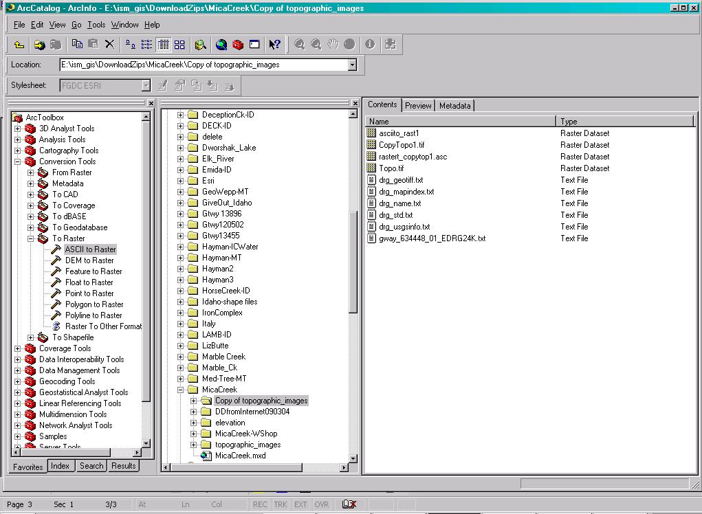
23 APPENDIX B (Return) Using ArcCatalog to trick (change) topographic rasters to correctly display in GeoWEPP when using Windows 2000 and ArcGIS 9.X. A. Changing the raster to ascii and then back to raster 1. In case of mistakes, make a copy of your original rasters to another folder. 2. Copy a topo (tif) file. In this example, I will name it CopyTopo1. 23

24 3. Change copytopo1 to an ascii file with ArcToolbox a. Under conversion tools > from raster > raster to ascii 24

25 4. Example file name => rastert_copytop1.asc (NOTE: you may have to change the name and keep track of which tif file you convert. ArcCatalog likes to name everything *.txt and 1 at the end. So you will have to change it to the correct topo file number and put asc at the end of the file. I have tried using the *.txt and could not get the tif file to project correctly.) 5. Next, change the ascii file back to raster a. Under conversion tools > to raster > ascii to raster b. Example file name => asciito_ras1 25

26 Default file name changed to asciito_ras1 26

27 B. Defining the raster 1. Select CopyTopo1 (the original file), right click and select properties. 2. Look under Spatial Reference and select Edit and then Import. 27

28 3. Select Import and navigate to new raster (asciito_ras1 see above example file name from above) and select this new raster file and click add, then OK and OK 4. The Spatial Reference portion of the CopyTopo1 file will now display <undefined> as the spatial reference. This is OK. CopyTopo1 will now display correctly with the elevation (NED) ascii in GeoWEPP. 5. Add the CopyTopo1 to your GeoWEPP simulation when the program asks for a topographic raster. DO NOT open up ArcMap and view your manipulated raster. ArcMap will change the raster and it will not overlay properly in GeoWEPP. Repeat as instructed under Part A and Part B as needed with remaining topographic rasters.topo 2, Topo 3 Topo 4 etc. NOTE: the topo maps may not overlay the NED exactly. But it will overlay close enough for you to know where you are at in the world. It is not critical that the topo overlays the NED exactly because the stream network is generated from the NED, not the topo map. And the stream network generated overlays nicely on the NED. 28

29 APPENDIX C (Return) Downloading a climate for use in WEPP Windows interface This example will describe how to download a 100 year climate near Tombstone, Arizona from the Forest Service WEPP web site. 1. Open web page 2. Select and click the Rock:Clime GUI (graphic user interface) 3. Select Arizona and click on the SHOW ME THE CLIMATES, button 4. Scroll down the list and select Tombstone. Click the MODIFY CLIMATE, button. 29

30 5. The following coordinates are located in the hills east of Tombstone, AZ. Type the following coordinates in the space provided: Lat = N and Long = W. Next, select the button 6. Below is the PRISM Precipitation screen. Note the grids on the right side of the screen for annual precipitation and elevation. The center cell is the climate for latitude 31.88N and longitude W. Think of these grids as layers, relating the similar positioned cells. For instance, the center cell on the top grid provides the precipitation for the elevation of the center cell in the bottom grid. The table on the left side of the screen is the precipitation table broken down by monthly average for both Tombstone and the new coordinates. 7. Select the Use PRISM Values, button. 30

31 8. Check the Adjust temperature for elevation by lapse rate (1,500 foot elevation difference) 9. Scroll down, type the name you wish to call your climate and save. The climate in this example is saved as Tombstone-mt-east 10. Your custom climate will show up under Personal Climate Stations. a. Type 100 in the space allotted for Number of Years of Climate b. Make sure you have your custom climate highlighted, as there will be other custom climates in the list (see figure below) c. Select DOWNLOAD CLIMATE 31

32 11. Save the file to the Arizona folder in the WEPP directory on your computer, figure below. C:\Program Files\USDA-ARS\WEPP\Data\climates\cligen\Arizona 12. Name your climate and select save. In this example, Tombstone-mt-east.txt. NOTE: In the event your computer will only allow you to save a *txt extension, you will need to navigate to the file location and manually change the file extension to *cli. In the Explore window of your computer, navigate to the saved climate text file: C:\Program Files\USDA-ARS\WEPP\Data\climates\cligen\Arizona in this example. 32

33 APPENDIX D (Return) Importing a climate for use in the WEPP Windows interface This example illustrates how to import a climate into the WEPP windows interface. 1. Open WEPP windows interface. 2. Start with a default project. 3. You will notice as you move the cursor around that it becomes a pointing hand when moved over the sun on the top-center portion of the screen. To import your custom climate into WEPP a. Position cursor/hand over sun b. RIGHT click and a drop down menu will appear. c. Select import 33

34 d. Navigate to your saved Tombstone-mt-east climate file: C:\Program Files\USDA-ARS\WEPP\Data\climates\cligen\Arizona e. Select your custom climate Tombstone-mt-east and click OK f. Tombstone-mt-east is now imported into WEPP windows. 34

35 APPENDIX E (Return) Quick Guide to WEPP Calibration and Saving Read Only Management Files 1. Open WEPP. 2. Change units to metric with the button under the main menu bar. Warning! You may run the model with English units, but realize, the results reported will vary due to rounding of significant figures between the Metric and English model. Metric = more significant figures. 3. Save model. File > Save as 4. Import a Climate file. Place the cursor over the sun icon located at the middle top of the display screen. When hovering, a pointing hand will appear. a. RIGHT click sun icon, select Import. 35

36 b. Navigate to your climate, select and click OK. In this example: cligen > Nevada > MtCharleston 5. Import a management file. Hover, the cursor over the top layer on the hillslope displayed in the middle of the display screen (dark green striped layer in the figure below). This layer represents the management file (otherwise known as a rotation = *.rot file). Another will show up over each of the three layers represented in the hillslope (top to bottom management, slope and soil). a. RIGHT click management layer, select Import and navigate to your management file. In this example: Managements > Forest > Disturbed WEPP Management > 30% Cover after fire 36

37 6. Import a slope file (optional). This is not a necessary step in the calibration process. But it is fun to have a different slope displayed. The little hand will appear over the middle layer (striped layer in figure below) RIGHT click, select Import and navigate to your slope file. In this example: Slopes > Disturbed WEPP slope > Disturbed WEPP-500, 30%, complex 7. Import a soil file. Place the cursor over the bottom layer (striped layer in figure below) and RIGHT click, select Import and navigate to desired soil file. In this example: Soils > Forest > Disturbed WEPP Soils > High sev fire sandy loam. 37

38 8. Change Run Options. The Run Options button is located on bottom center of screen. In WEPP Run Options Window, change Simulation years to 50 and check the box next to Return Period Summary or any other options you wish. 9. Run model. The Run button is located next to Run Options on the bottom center of the display. Once the simulation is run, several options are available along the bottom of the display screen. These options are grayed out in the figure below. 38

39 10. The model is finished running and the options along the bottom of the screen become available (figure below). This manual does not cover each of these options. But they are fairly easy to use, select and explore! Have fun! 11. Select Graphical Output button on bottom of the display screen. Select Graph 1. In the drop down menu, select the Days in Simulation on the x-axis and Interill cover (0-1) on the y-axis. Displaying the graph will allow you to look at the cover percent graphically as you change the different calibration parameters. Below the cover percent averages around 50%. 39

40 12. On the main menu select => Tools > Cover Calibration HINT: Select Help button for explanations regarding this tool. a. Change the Desired Cover to the cover percent you wish to achieve (in this example 30%), and click on the Calibrate button (figure below). b. After the Cover Calibration tool runs look under the Average Cover(%) column to check the true cover percent for the parameters given (Biomass Energy Ratio, Biomass Remaining Alter Senescence and Decomposition Rate HINT: Look in help menu for definitions). In this example, the 30% Cover after a fire calibrates to 50.5%. Adjusting the three parameters given; Biomass Energy Ratio (BER), Biomass Remaining After Senescence (BRAS) and Decomposition Rate (DR) will give you the Desired Cover (%). Normally, the DR is not changed. See the help file for explanation. 40

41 c. The BER and BRAS were changed until the Average Cover (%) equaled (or approximately equaled) the Desired Cover (%) 30% Vs 30.5%. NOTE: Changes in the BER and BRAS compared to the figure under 12a. Return to page 41, 48 d. Select the Accept button 13. Notice the difference in the graph Days of Simulation vs Interrill Cover is now approximately 30% (figure below). 14. Discussion of saving procedure: The next part of this exercise is to save the management file. Although WEPP appears to save the calibration file, I found that the file does not save properly and therefore, does not give correct results when using the file in GeoWEPP. 41

42 We will save it with a different name. If we name the file starting with a number, the new calibrated file will be near or at the top of the list in the rotation files directory. For this example, the new file name will be 30%Cover-MtCharleston or you may wish to create a folder for your calibration files. The easiest way to save the rotation files is to start with the most buried file and work backwards (Steps 15-39). When this part of the exercise is accomplished we must go back into the new management file (*.rot) and insert (or add) the Initial Conditions and Plant Database files. The second part of this procedure is outlined in steps Double click the management layer. 16. The first window is the Management Editor window. You will notice a file symbol under the 3 rd column between the Operation Type and Name. This is the Initial Conditions folder. 17. Double click the Initial Conditions folder. 18. You are now in the Initial Conditions Database window. There is another folder in the Initial Plant row under the Units column. 42

43 19. Double click the Initial Plant folder. 20. You are now in the Plant Database window. Check: Does the BER here match your calibrated BER? See Calibration Tool output window 12c. 21. Discussion: The Plant Database window is the final inner window or database level. This is the level we will start our Save As for the new calibration file. 22. Select the Save As button. 23. Type in the new name of your calibrated file. For this example, it is 30%Cover- MtCharleston. I also added my name and date in the Source field and added a description in the Comment field (figure below). 24. Select OK 43

44 25. The Plant Database window should now have your saved information at the top with the Plant Name, Description, Data Source and Comment (figure below). 26. Select Save 27. After the last save you are now back in the Initial Conditions Database window. 28. Select Save As in the Initial Conditions Database window. Enter the new Name of the calibration file 30%Cover-MtCharleston. Change the Source and Comments field if desired (figure below). 29. Select OK 44

45 30. You have now returned to the Initial Conditions Database window and the file has been updated with the new information (figure below). 31. Select Save. 32. After the last save you are back to the beginning, the Management Editor window. 45

46 33. In the Management Editor window at the bottom center of the window, change the Description to 30%Cover-MtCharleston. 34. Select Save As in the Management Editor window. 35. In the Save a WEPP management rotation window, name the *.rot file the same as the Initial Conditions and Plant Database files => 30%Cover-Mt.Charleston. 36. Save the *.rot file. 46

47 37. The next pop-up asks if you wish to use the new rotation file in the current selection (figure below). 38. Select yes. 39. Notice that the name on the layer has been changed from 30% Cover after fire to 30%Cover-MtCharleston. This is a result from changing the name in the description slot provided at the bottom of the Management Editor window, (see 33). Discussion: The new rotation file does not see the new Initial Conditions and the new Plant Database files we just saved. We must go back into the folder/window structure of the Management Editor window and change the Initial Conditions and Plant Database files to our new files. 40. Double click the management layer. Discussion: Notice, in the Management Editor window, the file under the Name column reads 30% Cover after fire NOT 30%Cover-Mt.Charleston. The new rotation file does not reflect the new Initial Conditions or Plant Database file we just save. We will retrieve the files. 47

48 41. Place your cursor on the right side of the row, under the Name column and left click on the mouse. A drop down menu will appear. Scroll to the new calibration file and select => 30%Cover-Mt.Charleston 42. The new file will automatically insert into the allotted slot under the Name column. 48

49 43. Select the Initial Conditions folder 44. You are in the Initial Conditions window. Again, there is a drop down menu, this time in the Value column. Select the drop down menu and navigate to your file => 30%Cover-MtCharleston. 45. Select the Initial Plant folder under the Units column. 49

50 46. Notice, the 30%Cover-MtCharleston file is in the Plant Database window! Awesome! Check: 1. Make sure BER matches your calibration data, 12c Make sure BRAS matches your calibration data, 12c 47. Check that the Plant Database window parameters are correct and select the Save button. 50

51 48. Now you are back in the Initial Conditions Database window Check: If you are using a different cover percent for example 20% or 35% - make sure you change these parameters in the Initial Conditions Database. There are 3 values that require changing. 49. Select Save in the Initial Conditions Database window. 50. A pop up window will ask you if you wish to Update initial conditions parameters? 51. Select the Yes button 51

52 52. Now we are back in the Management Editor window. 53. Select Save in the Management Editor window 54. The management file is now saved with the correct Initial Conditions Database and Plant Database files. 55. If you wish to recheck, repeat steps 41 through 56. I usually do just in case something flipped back. Is it always this difficult to save a rotation file (aka management file) in WEPP windows? Yes, it has always been this complicated to save the rotation file. Bill says that it has always been that way, something to do with the complexity of the model and the file structure. It is difficult process to automate but programmers are working on automation. You are now ready to go back through all of the above steps and calibrate a cover percent for your remaining treatments, whether thinning, prescribed burn or whatever. The best way to get accurate cover percents is through ground reconnaissance. The beauty of WEPP windows is that it allows the user access to all the parameters of the model. The user can then change any of these parameters to fit unique situations. The new management (*.rot) file we created 30%Cover-MtCharleston is now ready to use in GeoWEPP. In the future, if you decide to change any of the other parameters for this file, just select save. I always double check the file structure though to make sure it saved correctly. Remember if any portion of the file is read only you will need to duplicate the save procedure outlined above. It is advisable when calibrating covers to start with a like read only file (see page_15 this manual). This way you will ensure that all the parameters are the same. 52