Maxwell v Example (2D/3D Transient) Core Loss. Transformer Core Loss Calculation in Maxwell 2D and 3D

Transcription

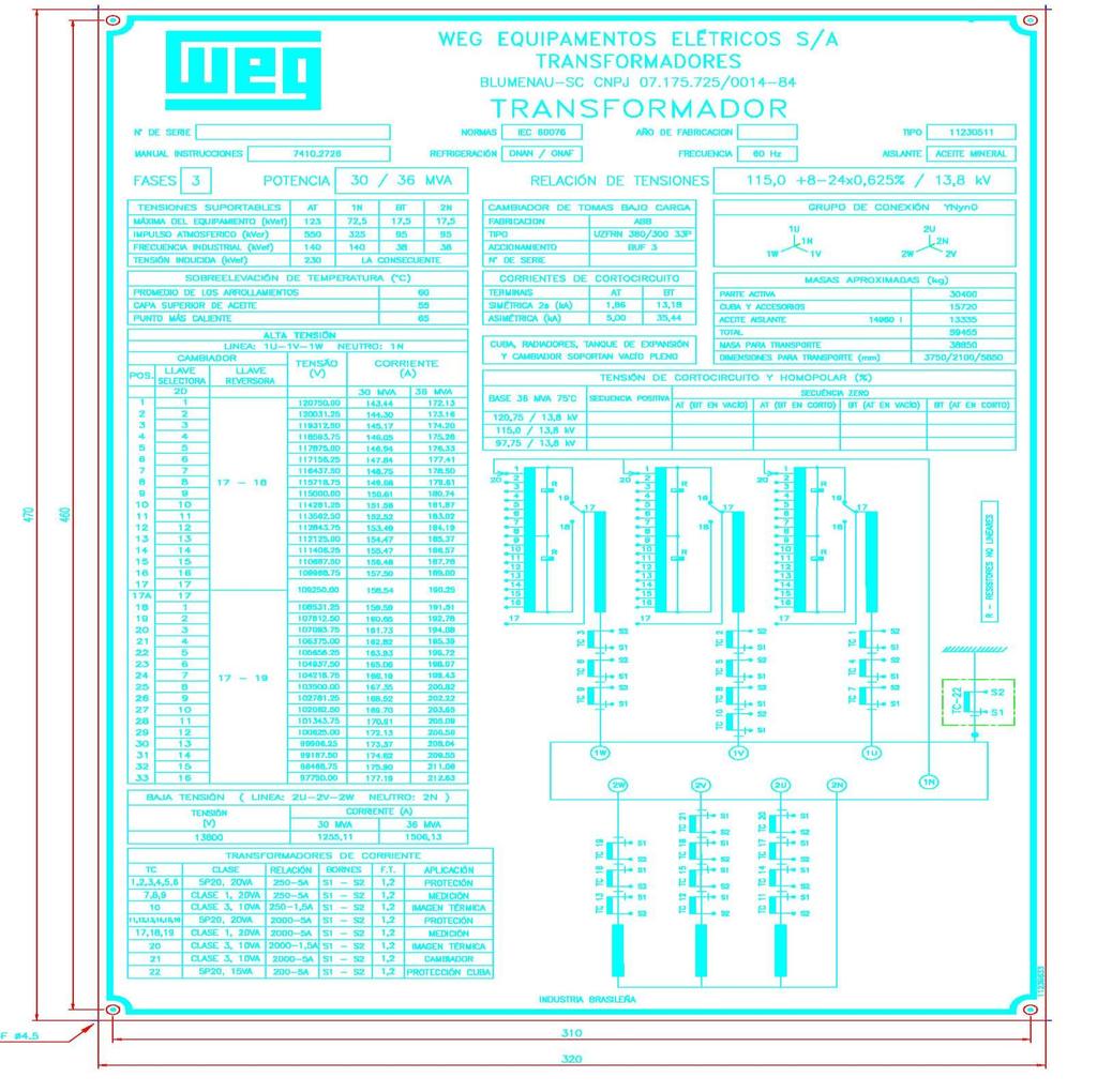
1 Transformer Core Loss Calculation in Maxwell 2D and 3D This example analyzes cores losses for a 3ph power transformer having a laminated steel core using Maxwell 2D and 3D. The transformer is rated kV, 60Hz and 30MVA. The tested power losses are 23,710W. It is important to realize that a finite element model cannot consider all of the physical and manufacturing core loss effects in a laminated core. These effects include: mechanical stress on laminations, edge burr losses, step gap fringing flux, circulating currents, variations in sheet loss values, to name just a few. Because of this the simulated core losses can be significantly different than the tested core losses. This example will go through all steps to create the 2D and 3D models based on a customer supplied base model. For core losses, only a single magnetizing winding needs to be considered. Core material will be characterized for nonlinear BH and core loss characteristics. An exponentially increasing voltage source will be applied in order to eliminate inrush currents and the need for an unreasonably long simulation time (of days or weeks). Finally, the core loss will be averaged over time and the core flux density will be viewed in an animated plot. This example will be solved in two parts using the 2D Transient and 3D Transient solvers. The model consists of a magnetic core and low voltage winding on each core leg. 3D Model 2D Model

2

3 Launch Maxwell To access Maxwell Click the Microsoft Start button, select Programs, and select Ansoft > Maxwell 15.0 and then Maxwell 15. Opening a New Project To Open a New Project After launching Maxwell, a project will be automatically created. You can also create a new project using below options. 1. In an Maxwell window, click the On the Standard toolbar, or select the menu item File > New. Select the menu item Project > Insert Maxwell 3D Design, or click on the icon Set Solution Type To Set Solution Type Select the menu item Maxwell 3D > Solution Type Solution Type Window: 1. Choose Magnetic > Transient 2. Click the OK button

4 Prepare Geometry To Import Geometry Select the menu item Modeler > Import Locate the parasolid file Ex_7_4_Core_Loss.x_t and Open it. The geometry is of a transformer with core simplified in order to reduce the complexity. Users can bring the geometries directly and do simplification inside Maxwell. Change Attributes Press Ctrl and select the objects LV_A, LV_B and LV_C and goto their properties window, 1. Change the color of the objects to Orange 2. Change the transparency of the objects to 0 Select the object Core from the history tree and goto Properties window, 1. Change the transparency of the object to 0 Specify Excitations To Create Coil Terminals Press Ctrl and select the objects LV_A, LV_B and LV_C Select the menu item Modeler > Surface Section In Section window, 1. Section Plane: Select XZ 2. Rename the resulting sections to SectionA, SectionB and SectionC respectively Select the sheets SectionA, SectionB and SectionC from the history tree Select the menu item Modeler > Boolean > Separate Bodies Delete the sheets SectionA_Separate1, SectionB_Separate1 and SectionC_Separate1

5 Assign Excitations Press Ctrl and select the sheets SectionA, SectionB and SectionC from the history tree Select the menu item Maxwell 3D > Excitations > Assign > Coil Terminal In Coil Terminal Excitation window, 1. Base Name: term_a 2. Number of Conductors: This will create three excitations corresponding to each section. Change their names as below: 1. Rename the excitation corresponding to SectionA as term_a Create Windings 2. Rename the excitation corresponding to SectionB as term_b 3. Rename the excitation corresponding to SectionC as term_c Select the menu item Maxwell 3D > Excitations > Add Winding In Winding window, 1. Name: WindingA 2. Type: Voltage 3. Stranded: Checked 4. Initial Current: 0 A 5. Resistance: 1 mohm 6. Inductance: 0 mh (Since this is calculated by solver) 7. Voltage: Vpeak*(1-exp(-50*time))*cos(2*pi*60*time) 8. In Add Variable window, 1. Unit Type: Voltage 2. Unit: V 3. Value: / 3 = Note: This is an exponentially increasing (in several cycles) sinusoidal 60Hz waveform with peak magnitude of 11,268V..

6 In Similar way add two more windings WindingB 1. Name: WindingB 2. Type: Voltage 3. Stranded: Checked 4. Initial Current: 0 A 5. Resistance: 1 mohm 6. Inductance: 0 mh (Since this is calculated by solver) 7. Voltage: Vpeak*(1-exp(-50*time))*cos(2*pi*60*time+(2/3*pi)) WindingC 1. Name: WindingC 2. Type: Voltage 3. Stranded: Checked 4. Initial Current: 0 A 5. Resistance: 1 mohm 6. Inductance: 0 mh (Since this is calculated by solver) 7. Voltage: Vpeak*(1-exp(-50*time))*cos(2*pi*60*time+(4/3*pi)) Add Terminals to Windings Expand the Project Manager tree to view Excitations Right click on WindingA and select Add Terminals In Add Terminals window, Select term_a In Similar way add term_b to WindingB Add term_c to WindingC

7 Assign Materials To Assign Materials to Coils Press Ctrl and select the objects LV_A, LV_B and LV_C, right click and select Assign Material In Select Definition window, 1. Type copper in Search by Name field 2. to assign material To Assign Material to Core Select the object Core from the history tree, right click and select Assign Material In Select Definition window, select the button Add Material In View/Edit Material window, Material Name: M125_027 Relative Permeability: Set the type to Nonlinear Select the button BH Curve from value field In BH Curve window, Select the button Import Dataset Set the File Type to *.Tab Locate the file Ex_7_4_core_loss_B_H.tab and Open it to close BH Curve window

8 Return to View/Edit Material window, Core Loss Type: Set to Electrical Steel Set the tab at the bottom of window Calculate Properties for to Core Loss at one Frequency In BP Curve window, Select the button Import Dataset Set the File Type to *.Tab Locate the file Ex_7_4_core_loss_B_loss.tab and Open it Core Loss Unit: w/kg Mass Density: 7650 kg/m^3 Frequency: 60 Hz Thickness: 0.27 mm Conductivity: S/m to close BP Curve window

9 Note that the core loss coefficients are calculated automatically. to create the new material to close Select Definition window Assign Mesh Operations In the transient solvers, there is no automatic adaptive meshing. Therefore, the user must either link the mesh from an identical model solved using the magnetostatic and eddy current solvers, or alternatively a manual mesh must be created. In this example, a mesh is created manually using inside selection to create elements throughout the volume of the objects. To Assign Mesh Operations for Core Select the object Core from the history tree Select the menu item Maxwell 3D > Mesh Operations > Assign > Inside Selection > Length Based In Element Length Based Refinement window, Name: Length_Core Restrict Length of Elements: Unchecked Restrict the Number of Elements: Checked Maximum Number of Elements: 10000

10 To Assign Mesh Operations for Coils Press Ctrl and select the objects LV_A, LV_B and LV_C from the history tree Select the menu item Maxwell 3D > Mesh Operations > Assign > Inside Selection > Length Based In Element Length Based Refinement window, Name: Length_Coils Restrict Length of Elements: Unchecked Restrict the Number of Elements: Checked Maximum Number of Elements: Set Core Loss Calculations To Set Core Loss calculations for Core Select the menu item Maxwell 3D > Excitations > Set Core Loss In Set Core Loss window, Core: Core Loss Settings: Checked Note: Once the core loss properties are defined in material definition, a tick mark will appear in the column Defined in Material indicating core loss coefficients are already specified

11 Set Eddy Effects Since winding is single object representing many strands and core is single object representing many laminations, eddy effect must be turned off them. To Turn off Eddy Effects in Objects Select the menu item Maxwell 3D > Excitations > Set Eddy Effects In Set Eddy Effects window, Ensure Eddy Effects are Unchecked for all objects Create Simulation Region To Create Region Select the menu item Draw > Region In Region window, Padding Data: Pad individual directions +/- X = 30 +/- Y = 200 +/- Z = 30 Note: This small padding % is acceptable as fields are completely concentrated inside the magnetic core and there is little or no fringing

12 Analysis Setup To Create Analysis Setup Select the menu item Maxwell 3D > Analysis Setup > Add Solution Setup In Solve Setup Window, General tab Stop time: 0.1s Time step: s Save Fields tab Type: Linear Step Start: 0.08 s Stop: 0.1 s Step Size: s Select the button Add to List >> Solver tab Nonlinear Residuals: 1e-6 (To Provide accurate convergence for BH Curve Save Analyze To Save File Select the menu item File > Save Save the file with the name Ex_7_4_Core_Loss.mxwl To Run Solution Select the menu item Maxwell 3D > Analyze All

13 Mesh Information To Plot Mesh on Core and Coils Select the object Region from the history tree Select the menu item View > Visibility > Hide Selection > Active View Select the menu item Edit > Select All Visible Select the menu item Maxwell 3D > Fields > Plot Mesh In Create Mesh Plot window, Press Done To View Mesh Information Select the menu item Maxwell 3D > Results > Solution Data In Solutions window, Select the tab Mesh Statistics to view mesh information

14 Create Reports Plot Winding Currents Vs Time Select the menu item Maxwell 3D > Results > Create Transient Report > Rectangular Plot In Report window, Category: Winding Quantity: Press Ctrl and select Current(WindingA), Current(WindingB) and Current(WindingC) Select New Report Note: Do not close Report window as we will create more plots using same window

15 Plot Input Voltages Vs Time In Report window, Quantity Deselect the Current quantities already selected Press Ctrl and select InputVoltage(WindingA), InputVoltage(WindingB) and InputVoltage(WindingC) Select New Report Plot Cores Loss vs Time In Report window, Category: Change to Loss Quantity: Select CoreLoss Select New Report Press Close to close report window

16 Calculate Avg Losses over a Time Range In XY Plot Corresponding to CoreLoss, right click on the Legend and select Trace Characteristics > Add In Add Trace Characteristics window, Category: Math Function: Avg Change the Range from Full to Specified Start of Range: 80 ms End of Range: 100 ms Select Add and Done

17 Create Flux Density Plot To Plot Flux Density on Core Double click on Maxwell3DDesign1 in Project Manager window to exit Plot view Select the object Core from the history tree Select the menu item Maxwell 3D > Fields > Fields > B > Mag_B In Create Field Plot window, Plot on surface Only: Checked Press Done

18 To Animate the Plot Select the menu item Maxwell 3D > Fields > Animate In Setup Animation window, Sweep Variable: Time Select values: Select the time range from s to 0.087s An Animation window will pop up which will enable to start, stop, pause the animation. Animation speed can also be varied using same window. The animation can be also exported in GIF or AVI format using Export button

19 Part 2: 2D Eddy Project Create a 2D Design Automatically To Create a 2D Design from 3D Select the menu item Maxwell 3D > Create 2D Design In Create 2D Design window, Coordinate System: Global Section Plane: ZX 2D Geometry Mode: XY Set Solution Type To Set Solution Type Select the menu item Maxwell 2D > Solution Type In Solution Type window, Verify that Geometry Mode is set to Cartesian, XY Select the radio button to Magnetic > Transient Set Model Depth Set the depth of the 2D XY model to give the same area as in Maxwell 3D = mm 2. Since the width of the core leg = 580mm, set the depth = 456mm. To Set Model Depth Select the menu item Maxwell 2D > Model > Set Model Depth In Design Settings window, Set Model Depth to 456 mm

20 Modify 2D Geometry Modify Region Expand the history tree corresponding to the sheet Region Double click on the command CreateRegion from the history tree In Properties window, Change +X Padding Data to 100 Change X Padding Data to 100 Delete Unnecessary Sheets Press Ctrl and select the sheets SectionA, SectionB and SectionC Select the menu item Edit > Delete Separate Coil Sections Press Ctrl and select the sheets LV_A,LV_B and LV_C Select the menu item Modeler > Boolean > Separate Bodies

21 Specify Excitations Assign Coil: Out Press Ctrl and select the sheets LV_A, LV_B and LV_C from history tree Select the menu item Maxwell 2D > Excitations > Assign > Coil In Coil Excitation window, Base Name: out Number of Conductors: 76 Polarity: Positive Rename the excitations created to A_out, B_out and C_out Assign Coil: In Press Ctrl and select the sheets LV_A_Separate1, LV_B_Separate1 and LV_C_Separate1 from history tree Select the menu item Maxwell 2D > Excitations > Assign > Coil In Coil Excitation window, Base Name: in Number of Conductors: 76 Polarity: Negative Rename the excitations created to A_in, B_in and C_in Add Windings Select the menu item Maxwell 2D > Excitations > Add Winding In Winding window, 1. Name: WindingA 2. Type: Voltage 3. Stranded: Checked 4. Initial Current: 0 A 5. Resistance: 1 mohm 6. Inductance: 0 mh (Since this is calculated by solver) 7. Voltage: Vpeak*(1-exp(-50*time))*cos(2*pi*60*time) 8. In Add Variable window, 1. Unit Type: Voltage 2. Unit: V 3. Value: / 3 =

22 In Similar way add two more windings WindingB 1. Name: WindingB 2. Type: Voltage 3. Stranded: Checked 4. Initial Current: 0 A 5. Resistance: 1 mohm 6. Inductance: 0 mh (Since this is calculated by solver) 7. Voltage: Vpeak*(1-exp(-50*time))*cos(2*pi*60*time+(2/3*pi)) WindingC 1. Name: WindingC 2. Type: Voltage 3. Stranded: Checked 4. Initial Current: 0 A 5. Resistance: 1 mohm 6. Inductance: 0 mh (Since this is calculated by solver) 7. Voltage: Vpeak*(1-exp(-50*time))*cos(2*pi*60*time+(4/3*pi)) Add Coils to the Winding Expand the Project Manager tree to view Excitations Right click on WindingA and select Add Coils In Add Terminals window, Press Ctrl and select A_in and A_out In Similar way add B_in and B_out to WindingB Add C_in and C_out to WindingC

23 Assign Boundary The current is assumed to be 1A at 0 degrees in the left busbar and -1A at 60 degrees in the right busbar. A no-fringing vector potential boundary will be assigned to the outside of the 2D problem region which is also the default boundary for all 3D projects. This forces all flux to stay in the solution region. To Assign Boundary Select the menu item Edit > Select > Edges Select all external edges of the Region Select the menu item Maxwell 2D > Boundaries > Assign > Vector Potential In Vector Potential Boundary window, Value: Set to 0 Select the menu item Edit > Select > Objects to change selection filter Assign Mesh Operations As in the 3D transient solver, there is no adaptive meshing in the 2D transient solver. A manual mesh is created manually using inside selection to create elements throughout the volume of the objects. To Assign Mesh Operation Press Ctrl and select the core and all six sheets corresponding to coils Select the menu item Maxwell 2D > Mesh Operations > Assign > Inside Selection > Length Based Set Eddy Effects In Element Length Based Refinement window, Restrict Length of Elements: Checked Maximum Length of Elements: 100 mm Restrict the Number of Elements: Unchecked To Turn off Eddy Effects in Objects Select the menu item Maxwell 2D > Excitations > Set Eddy Effects In Set Eddy Effects window, Ensure Eddy Effects are Unchecked for all objects

24 Set Core Loss Calculations To Set Core Loss calculations for Core Select the menu item Maxwell 2D > Excitations > Set Core Loss In Set Core Loss window, Core: Core Loss Settings: Checked Analysis Setup Save Analyze To Create Analysis Setup Select the menu item Maxwell 2D > Analysis Setup > Add Solution Setup In Solve Setup Window, General tab Stop time: 0.1s Time step: s Save Fields tab Type: Linear Step Start: 0.08 s Stop: 0.1 s Step Size: s Select the button Add to List >> Solver tab Nonlinear Residuals: 1e-6 To Save File Select the menu item File > Save To Run Solution Select the menu item Maxwell 3D > Analyze All

25 Mesh Information To Plot Mesh on Core and Coils Select the menu item Edit > Select All Visible Select the menu item Maxwell 2D > Fields > Plot Mesh In Create Mesh Plot window, Press Done To View Mesh Information Select the menu item Maxwell 2D > Results > Solution Data In Solutions window, Select the tab Mesh Statistics to view mesh information

26 Create Reports Plot Winding Currents Vs Time Select the menu item Maxwell 2D > Results > Create Transient Report > Rectangular Plot In Report window, Category: Winding Quantity: Press Ctrl and select Current(WindingA), Current(WindingB) and Current(WindingC) Select New Report Note: Do not close Report window as we will create more plots using same window

27 Plot Input Voltages Vs Time In Report window, Quantity Deselect the Current quantities already selected Press Ctrl and select InputVoltage(WindingA), InputVoltage(WindingB) and InputVoltage(WindingC) Select New Report Plot Cores Loss vs Time In Report window, Category: Change to Loss Quantity: Select CoreLoss Select New Report Press Close to close report window

28 Calculate Avg Losses over a Time Range In XY Plot Corresponding to CoreLoss, right click on the Legend and select Trace Characteristics > Add In Add Trace Characteristics window, Category: Math Function: Avg Change the Range from Full to Specified Start of Range: 80 ms End of Range: 100 ms Select Add and Done

29 Create Flux Density Plot To Plot Flux Density on Core Double click on Maxwell2DDesign1 in Project Manager window to exit Plot view Select the sheet Core from the history tree Select the menu item Maxwell 2D > Fields > Fields > B > Mag_B In Create Field Plot window, Press Done

30 To Animate the Plot Select the menu item Maxwell 2D > Fields > Animate In Setup Animation window, Sweep Variable: Time Select values: Select the time range from s to 0.087s An Animation window will pop up which will enable to start, stop, pause the animation. Animation speed can also be varied using same window. The animation can be also exported in GIF or AVI format using Export button