THE fast and reliable estimation of the pose of the human
|
|
|
- Ashlynn Walker
- 6 years ago
- Views:
Transcription
1 TRANS. PAMI, SUBMITTED FOR REVIEW, Efficient Human Pose Estimation from Single Depth Images Jamie Shotton, Member, IEEE, Ross Girshick, Andrew Fitzgibbon, Senior Member, IEEE, Toby Sharp, Senior Member, IEEE, Mat Cook, Mark Finocchio, Richard Moore, Member, IEEE, Pushmeet Kohli, Antonio Criminisi, Alex Kipman, Andrew Blake, Fellow, IEEE (Invited Paper - CVPR 2011 special issue) Abstract We describe two new approaches to human pose estimation. Both can quickly and accurately predict the 3D positions of body joints from a single depth image, without using any temporal information. The key to both approaches is the use of a large, realistic, and highly varied synthetic set of training images. This allows us to learn models that are largely invariant to factors such as pose, body shape, field-of-view cropping, and clothing. Our first approach employs an intermediate body parts representation, designed so that an accurate per-pixel classification of the parts will localize the joints of the body. The second approach instead directly regresses the positions of body joints. By using simple depth pixel comparison features, and parallelizable decision forests, both approaches can run super-realtime on consumer hardware. Our evaluation investigates many aspects of our methods, and compares the approaches to each other and to the state of the art. Results on silhouettes suggest broader applicability to other imaging modalities. Index Terms Computer vision, Machine learning, Pixel classification, Depth cues, Range data, Games. 1 INTRODUCTION THE fast and reliable estimation of the pose of the human body from images has been a goal of computer vision for decades. Robust interactive pose estimation has applications including gaming, human-computer interaction, security, telepresence, and even health-care. The recent availability of high-speed depth sensors has greatly simplified the task [1], [2], [3], [4], [5], [6]. However, until the launch of the Microsoft Kinect camera and gaming platform [7] in November 2010, even the best systems exhibited failures when faced with unusual poses, occlusion, sensor noise, and the constraints of super-realtime operation (i.e. with a budget of a fraction of the total processor cycles). This paper describes some of the research behind a core component of the skeletal tracking pipeline that ships in with Kinect [7]. The aim to ship a consumer product necessitated two important design goals: robustness and computational efficiency. We wanted to build something that could work without calibration for any human body shape, so that anyone could start using the system immediately. The system also had to be able to run for hours at a time without failing catastrophically. Our final requirements came in the form of tight budgets for compute and memory usage. Towards these goals, this paper presents two related approaches for estimating human pose, illustrated in Fig. 1. We will refer to these as body part classification This work was undertaken at Microsoft Research, Cambridge, in collaboration with Xbox. See R. Girshick is currently a postdoctoral fellow at UC Berkeley. R. Moore is currently working at ST-Ericsson. (BPC) and offset joint regression (OJR). The BPC and OJR algorithms output high-quality shortlists of confidenceweighted proposals for the 3D locations of the skeletal body joints. These proposals are computed at each frame and for each joint independently. Traditional human body tracking algorithms [8], [9], [1], [10], [6], [11] infer a complete skeleton by exploiting kinematic constraints and can achieve high framerates by using temporal coherence from frame-to-frame. However, without regular re-initialization, tracking algorithms are prone to catastrophic loss of track. Our original design was for our 3D body joint proposals to provide initialization and per-frame recovery to complement any appropriate tracking algorithm. However, our per-frame, per-joint proposals have proven remarkably accurate, and might well be usable without tracking a full body model. Both BPC and OJR use an efficient decision forest that is applied at each pixel in the image. Evaluating the contribution of each pixel to each joint separately avoids any combinatorial search over body joints. The forest uses simple yet discriminative depth comparison image features that give 3D translation invariance while maintaining high computational efficiency. In an optimized implementation, these features and the classifier itself can be evaluated in parallel across each pixel on a GPU [12] or multi-core CPU. Both algorithms can run at superrealtime rates on consumer hardware, leaving sufficient computational resources to allow complex game logic and graphics to run in parallel. The two methods also share their use of a very large, realistic, synthetic training corpus, generated by rendering depth images of humans. Each render is assigned
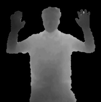
![TRANS. PAMI, SUBMITTED FOR REVIEW, 2012 2 input depth image BPC body parts mean shift [19] to give the final set of 3D body joint proposals.](/docs-images/74/71375571/images/2-0.jpg "Optimized implementations of our algorithms can run at around 200 frames per second on consumer hardware, at least one order of magnitude faster than existing approaches.")


 first predicts a (colorcoded) body part label at each pixel, and then uses these inferred labels to localize the body joints.")
2 TRANS. PAMI, SUBMITTED FOR REVIEW, input depth image BPC body parts mean shift [19] to give the final set of 3D body joint proposals. Optimized implementations of our algorithms can run at around 200 frames per second on consumer hardware, at least one order of magnitude faster than existing approaches. To validate our algorithms, we evaluate on both real and synthetic depth images, containing challenging poses of a varied set of subjects. Even without exploiting temporal or kinematic constraints, the 3D body joint proposals are both accurate and stable. We investigate the effect of several training parameters and show a substantial improvement over the state of the art. Further, preliminary results on silhouette images suggest more general applicability of our approach to scenarios where depth cameras are not available. front view side view top view body joint positions Fig. 1. Method overview on ground truth example. Body part classification (BPC) first predicts a (colorcoded) body part label at each pixel, and then uses these inferred labels to localize the body joints. Offset joint regression (OJR) instead more directly regresses the positions of the joints. The input depth point cloud is shown overlaid on the body joint positions for reference. randomly sampled parameters including body shape, size, pose, scene position, etc. We can thus quickly and cheaply generate hundreds of thousands of varied images with associated ground-truth (the body part label images and the set of 3D body joint positions). This allows us to train deep forests, without the risk of overfitting, that can naturally handle a full range of human body shapes undergoing general body motions [13], self-occlusions, and poses cropped by the image frame. Body part classification, originally published in [14], was inspired by recent object recognition work that divides objects into parts (e.g. [15], [16], [17], [5]). BPC uses a randomized classification forest to densely predict discrete body part labels across the image. Given the strong depth image signal, no pairwise terms or CRF have proved necessary for accurate labeling. The pattern of these labels is designed such that the parts are spatially localized near skeletal joints of interest. Given the depth image and the known calibration of the depth camera, the inferred per-pixel label probabilities can be reprojected to define a density over 3D world space. Offset joint regression [18] instead employs a randomized regression forest to directly cast a set of 3D offset votes from each pixel to the body joints. These votes are used to again define a world space density. Modes of these density functions can be found using 1.1 Contributions Our main contribution are as follows. We demonstrate that using efficient machine learning approaches, trained with a large-scale, highly varied, synthetic training set, allows one to accurately predict the positions of the human body joints in super-realtime. We show how a carefully designed pattern of body parts can transform the hard problem of pose estimation into an easier problem of per-pixel semantic segmentation. We examine both classification and regression objective functions for training the decision forests, and obtain slightly surprising results that suggest a limitation of the standard regression objective. We employ regression models that compactly summarize the pixel-to-joint offset distributions at leaf nodes. We show that these make our method both faster and more accurate than Hough Forests [20]. We will refer to this as vote compression. This paper builds on our earlier publications [14], [18]. It unifies the notation, explains the approaches in more detail, and includes a considerably more thorough experimental validation. 1.2 Depth imaging Depth imaging technology has advanced dramatically over the last few years, and has finally reached a consumer price point [7]. Pixels in a depth image indicate the calibrated distance in meters of 3D points in the world from the imaging plane, rather than a measure of intensity or color. We employ the Kinect depth camera (and simulations thereof) to provide our input data. Kinect uses structured infra-red light and can infer depth images with high spatial and depth resolution at 30 frames per second. Using a depth camera gives several advantages for human pose estimation. Depth cameras work in low light conditions (even in the dark), help remove ambiguity in scale, are largely color and texture invariant, and resolve
3 TRANS. PAMI, SUBMITTED FOR REVIEW, silhouette ambiguities. They also greatly simplify the task of background subtraction which we assume in this work as a pre-processing step. Most importantly for our approach, since variations in color and texture are not imaged, it is much easier to synthesize realistic depth images of people and thus cheaply build a large training dataset. 1.3 Related Work Human pose estimation has generated a vast literature, surveyed in [21], [22]. We briefly review some of the recent advances Recognition in parts Several methods have investigated using some notion of distinguished body parts. One popular technique, pictorial structures [23], was applied by Felzenszwalb & Huttenlocher [24] to efficiently estimate human pose by representing the body by a collection of parts arranged in a deformable configuration. Springs are used between parts to model the deformations. Ioffe & Forsyth [25] group parallel edges as candidate body segments and prune combinations of segments using a projected classifier. Ramanan & Forsyth [26] find candidate body segments as pairs of parallel lines and cluster their appearances across frames, connecting up a skeleton based on kinematic constraints. Sigal et al. [9] use eigenappearance template detectors for head, upper arms and lower legs proposals. Non-parametric belief propagation was then used to infer whole body pose. Tu s autocontext was used in [27] to obtain a coarse body part labeling. These labels were not defined to localize joints, and classifying each frame took about 40 seconds. Poselets that form tight clusters in both 3D pose and 2D image appearance, detectable using SVMs, were presented by Bourdev & Malik [17]. Wang & Popović [10] proposed a related approach to track a hand clothed in a colored glove; our BPC system could be viewed as automatically inferring the colors of a virtual colored suit from a depth image. As detailed below, our BPC algorithm [14], extends the above techniques by using parts that densely cover the body and directly localize body joints Pose from depth Recent work has exploited improvements in depth imaging and 3D input data. Anguelov et al. [28] segment puppets in 3D range scan data into head, limbs, torso, and background using spin images and a MRF. Grest et al. [1] use Iterated Closest Point (ICP) to track a skeleton of a known size and starting position from depth images. In [3], Zhu & Fujimura build heuristic detectors for coarse upper body parts (head, torso, arms) using a linear programming relaxation, but require a T-pose initialization to calibrate the model shape. Siddiqui & Medioni [4] hand-craft head, hand, and forearm detectors, and show that data-driven MCMC model fitting outperforms the iterated closest point algorithm. Kalogerakis et al. [29] classify and segment vertices in a full closed 3D mesh into different parts, but do not deal with occlusions and are sensitive to mesh topology. Plagemann et al. [5] build a 3D mesh to find geodesic extrema interest points which are classified into 3 parts: head, hand, and foot. This method provides both a location and orientation estimate of these parts, but does not distinguish left from right, and the use of interest points limits the choice of parts Regression Regression has been a staple of monocular 2D human pose estimation [30], [31], [32], [13]. Several methods have explored matching exemplars or regressing from a small set of nearest neighbors. The shape context descriptor was used by Mori & Malik [33] to retrieve exemplars. Shakhnarovich et al. [34] estimate upper body pose, interpolating k-nn poses efficiently indexed by parameter sensitive hashing. Agarwal & Triggs [30] learn a regression from kernelized image silhouette features to pose. Navaratnam et al. [32] use the marginal statistics of unlabeled data to improve pose estimation. Local mixtures of Gaussian Processes were used by Urtasun & Darrell [13] to regress human pose. Our OJR approach combines some ideas from these approaches with the tools of high-speed object recognition based on decision trees Other approaches An alternative random forest based method for pose estimation was proposed by [35]. Their approach quantizes the space of rotations and gait cycle, though does not directly produce a detailed pose estimate. A related technique to our OJR algorithm is used in object localization. For example, in the implicit shape model (ISM) [36], visual words are used to learn voting offsets to predict 2D object centers. ISM has been extended in two pertinent ways. Müller et al. [37] apply ISM to body tracking by learning separate offsets for each body joint. Gall and Lempitsky [20] replace the visual word codebook of ISM by learning a random forest in which each tree assigns every image pixel to a decision-tree leaf node at which is stored a potentially large collection of votes. This removes the dependence of ISM on repeatable feature extraction and quantization, as well as the somewhat arbitrary intermediate codebook representation. Associating a collection of vote offsets with each leaf node/visual word, these methods then accumulate votes to determine the object centers/joint positions. Our OJR method builds on these techniques by compactly summarizing the offset distributions at the leaf nodes, learning the model hyper-parameters, and using a continuous test-time voting space. 1.4 Outline The remainder of the paper is organized as follows. Sec. 2 explains how we generate the large, varied train-
4 TRANS. PAMI, SUBMITTED FOR REVIEW, ing set that is the key to our approach. Following that, Sec. 3 describes the two algorithms in a unified framework. Our experimental evaluation is detailed in Sec. 4, and we conclude in Sec DATA Many techniques for pose estimation require training images with high quality ground truth labels, such as joint positions. For real images, these labels can be very expensive to obtain. Much research has thus focused on techniques to overcome lack of training data by using computer graphics [34], [38], [39], but there are two potential problems: 1) Rendering realistic intensity images is hampered by the huge color and texture variability induced by clothing, hair, and skin, often meaning that the data are reduced to 2D silhouettes [30]. While depth cameras significantly reduce this difficulty, considerable variation in body and clothing shape remains. 2) Synthetic body pose renderers use, out of necessity, real motion capture (mocap) data. Although techniques exist to simulate human motion (e.g. [40]) they do not yet produce a full range of volitional motions of a human subject. In this section we describe how we overcome these problems. We take real mocap data, retarget this to a variety of base character models, and then synthesize a large, varied dataset. We believe the resulting dataset to considerably advance the state of the art in both scale and variety, and will demonstrate the importance of such a large dataset in our evaluation. 2.1 Motion capture data As noted above, simulating human pose data is an unsolved problem. Instead, we obtain ground truth pose data using marker-based motion capture of real human actors. The human body is capable of an enormous range of poses. Modeled jointly, the number of possible poses is exponential in the number of articulated joints. We cannot thus record all possible poses. However, there is hope. As will be seen in Sec. 3, our algorithms, based on sliding window decision forests, were designed to only look at a local neighborhood of a pixel. By looking at local windows, we factor whole body poses into combinations of local poses, and can thus expect the forests to generalize somewhat to unseen poses. In practice, even a limited corpus of mocap data where for example each limb separately moves through a wide range of poses has proven sufficient. Further, we need not record mocap with variation in rotation about the vertical axis, mirroring left-right, scene position, body shape and size, or camera pose, all of which can be simulated. Given our core entertainment scenario, we recorded 500K frames in a few hundred sequences of driving, dancing, kicking, running, navigating menus, etc. To create training data we render single, static depth images because, as motivated above, our algorithms deliberately eschew temporal information. Often, changes in pose from one mocap frame to the next are so small as to be insignificant. We can thus discard many similar, redundant poses using furthest neighbor clustering [41]. We represent a pose P as a collection P = (p 1,..., p J ) of J joints where each p j is a 3D position vector. Starting with set P all of all the recorded mocap poses, we choose an initial pose at random and then greedily grow a set P as P := P { argmax min d pose(p, P ) }, (1) P P P P all \P where as the distance between poses we use the maximum Euclidean distance over body joints j d pose (P, P ) = max j {1,...,J} p j p j 2. (2) We stop growing set P when there exists no unchosen pose P which has d pose (P, P ) > D pose for any chosen pose P. We set D pose = 5cm. This results in a final subset P P all containing approximately 100K most dissimilar poses. We found it necessary to iterate the process of motion capture, rendering synthetic training data, training the classifier, and testing joint prediction accuracy. This allowed us to refine the mocap database with regions of pose space that had been previously missed out. Our early experiments employed the CMU mocap database [42] which gave acceptable results though covers far less of pose space. 2.2 Rendering synthetic data We build a randomized rendering pipeline. This can be viewed as a generative model from which we can sample fully labeled training images of people. Our goals in building this pipeline were twofold: realism we want the samples to closely resemble real images so that the learned model can work well on live camera input; and variety the dataset must contain a good coverage of the appearance variations we hope to recognize at test time. Fig. 3 illustrates the huge space of possible appearance variations we need to deal with for just one body part, even when restricted to a pixel s local neighborhood as discussed above. Our features achieve 3D translation invariance by design (see below). However, other invariances such as pose and shape cannot be designed so easily or efficiently, and must instead be encoded implicitly through the training data. The rendering pipeline thus randomly samples a set of parameters, using the best approximations we could reasonably achieve to the variations we expected to observe in the real world. While we cannot hope to sample all possible combinations of variations, if samples contain somewhat independent variations (in particular, excluding artificial correlations such as thin people always wear a hat), we can expect the classifier


.")


5 real (test) 5 synthetic (train & test) TRANS. PAMI, SUBMITTED FOR REVIEW, 2012 Right hand appearances Fig. 2. Synthetic vs. real data. Pairs of depth images and corresponding color-coded ground truth body part label images. The 3D body joint positions are also known (but not shown). Note wide variety in pose, shape, clothing, and crop. The synthetic images look remarkably similar to the real images, lacking primarily just the high-frequency texture. Base Character Models Fig. 3. A single body part varies widely in its context. to learn a large degree of invariance. Let us run through the variations we simulate: Base Character. We use 3D models of 15 varied base characters, both male and female, from child to adult, short to tall, and thin to fat. Some examples are shown in Fig. 4. A given render will pick uniformly at random from the characters. Pose. Having discarded redundant poses from the mocap data, we retarget the remaining poses P P to each base character using [43]. A pose is selected uniformly at random and mirrored left-right with probability 12 to prevent a left or right bias. Rotation & Translation. The character is rotated about the vertical axis and translated in the scene, uniformly at random. Translation ensures we obtain cropped training examples where the character is only partly in-frame. Hair & Clothing. We add mesh models of several hair styles and items of clothing chosen at random. A slight gender bias is used, so that, for instance, long hair is chosen more often for the female models, and beards are only chosen for the male models. Weight & Height Variation. The base characters already include a wide variety of weights and heights. To add further variety we add an extra variation in height (±10%) and weight (±10%). For rendering efficiency, we assume this variation does not affect the pose retargetting. Camera Position & Orientation. The camera height, pitch and roll are chosen uniformly at random within a range believed to be representative of an entertainment scenario in a home living room. Camera Noise. While depth camera technology has improved rapidly in the last few years, real depth cameras exhibit noise, largely due to non-ir-reflecting materials (e.g. glass, hair), surfaces that are almost perpendicular Fig. 4. Example base character models. to the sensor, and ambient illumination. To ensure high realism in our dataset, we thus add artificial noise to the clean computer graphics renders to simulate the depth imaging process: dropped-out pixels, depth shadows, spot noise and disparity quantization. We use standard linear skinning techniques from computer graphics to animate the chosen 3D mesh model given the chosen pose, and a custom pixel shader is used to render the depth images. Fig. 2 compares the varied output of the pipeline to hand-labeled real depth images. The synthetic data is used both as fully labeled training data, and, alongside real hand-labeled depth images, as test data in our evaluation. In building this randomized rendering pipeline, we attempted to fit as much variety in as many ways as we could, given the time constraints we were under. Investigating the precise effects of the choice and amounts of variation would be fascinating, but lies beyond the scope of this work. 2.3 Training data labeling A major advantage of using synthetic training images is that the ground truth labels can be generated almost for free, allowing one to scale up supervised learning to very large scales. The complete rendering pipeline allows us to rapidly sample hundreds of thousands of unique images of people. The particular tasks we address in this work, BPC and OJR, require different types of label, described next.
.")

6 Image Features TRANS. PAMI, SUBMITTED FOR REVIEW, Body part classification labels Our first algorithm, BPC, aims to predict a discrete body part label at each pixel. At training time, these labels are required for all pixels, and we thus represent the labels as a color-coded body part label image that accompanies each depth image (see Figs. 1 and 2). The use of an intermediate body part representation that can localize 3D body joints is a key contribution of this work. It transforms the pose estimation problem into one that can readily be solved by efficient classification algorithms. The particular pattern of body parts used was designed by hand to balance these desiderata: the parts must densely cover the body, as a prediction is made for every pixel in the foreground; the parts should not be so small and numerous as to waste capacity of the classifier; and the parts must be small enough to well localize a region of the body. By centering and localizing some of the parts around body joints of interest, accurate body part predictions will necessarily spatially localize those body joints, and, because we have calibrated depth images, this localization will implicitly be in 3D. The parts definition can be specified in a texture map and retargetted to the various 3D base character meshes for rendering. For our experiments, we define 31 body parts: LU/RU/LW/RW head, neck, L/R shoulder, LU/RU/LW/RW arm, L/R elbow, L/R wrist, L/R hand, LU/RU/LW/RW torso, LU/RU/LW/RW leg, L/R knee, L/R ankle, and L/R foot (Left, Right, Upper, lower). Distinct parts for left and right allow the classifier to learn to disambiguate the left and right sides of the body. The precise definition of these parts might be changed to suit a particular application. For example, in an upper body tracking scenario, all the lower body parts could be merged into a single part Offset joint regression labels Our second algorithm, OJR, instead aims to estimate the 3D joint positions more directly. As such, the ground truth labels it requires are simply the ground truth 3D joint positions. These are trivially recorded during the standard mesh skinning process. In our experiments, we use 16 body joints: head, neck, L/R shoulder, L/R elbow, L/R wrist, L/R hand, L/R knee, L/R ankle, and L/R foot. This selection allows us to directly compare the BPC and OJR approaches on a common set of predicted joints. 3 METHOD Our algorithms cast votes for the position of the body joints by evaluating a sliding window decision forest at each pixel. These votes are then aggregated to infer reliable 3D body joint position proposals. In this section we describe: (i) the features we employ to extract discriminative information from the image; (ii) the structure of a random forest, and how it combines multiple such features to achieve an accurate set of votes; (iii) the (a) φ 2 φ 1 (b) Fig. 5. Depth image features. The yellow crosses indicate the image pixel u being classified. The red circles indicate the offset pixels as defined in Eq. 3. In (a), the two example features give a large depth difference response, i.e. f(u φ) is large. In (b), the same two features at new image locationsθ 2 give a much smaller response. θ In 2 practice, many such features combined in a decision forest give a strong discriminative signal. different leaf node prediction models used for BPC and OJR; (iv) how the pixel votes are aggregated into a set of joint position predictions at test time; and (iv) how the forests are learned. 3.1 Depth image features We employ simple depth comparison features, inspired by those in [44]. Individually these features provide only a weak discriminative signal, but combined in a decision forest they prove sufficient to accurately disambiguate different appearances and regions of the body. At a given pixel u, the feature response is computed as f(u φ) = z ( u + δ 1 z(u) ) z φ 1 ( u + δ 2 z(u) ) φ 2, (3) where feature parameters φ = (δ 1, δ 2 ) describe 2D pixel offsets δ, and function z(u) looks up the depth at pixel u = (u, v) in a particular image. Each feature therefore performs two offset depth probes in the image and takes their difference. The normalization of the offsets by 1 z(u) ensures that the feature response is depth invariant: at a given point on the body, a fixed world space offset will result whether the depth pixel is close or far from the camera. The features are thus 3D translation invariant, modulo perspective effects. If an offset pixel u lies on the background or outside the bounds of the image, the depth probe z(u ) is assigned a large positive constant value. During training of the tree structure, offsets δ are sampled at random within a box of fixed size. We investigate sampling strategies in Sec , and evaluate the effect of this maximum depth probe offset in Fig. 11(c). We further set δ 2 = 0 with probability 1 2. This means that roughly half the features evaluated are unary (look at only one offset pixel) and half are binary (look at two offset pixels). In practice the results appear to be fairly insensitive to this parameter. Fig. 5 illustrates two different features. The unary feature with parameters φ 1 looks upwards: Eq. 3 will
7 Random Forests TRANS. PAMI, SUBMITTED FOR REVIEW, tree 1 u l 1 u l T u u tree T Fig. 6. Randomized Decision Forests. A forest is an ensemble of T decision trees. Each tree consists of split nodes (blue) and leaf nodes (green). The red arrows indicate the different paths that might be taken by different trees for a particular input. give a large positive response for pixels u near the top of the body, but a value close to zero for pixels u lower down the body. By similar reasoning, the binary feature (φ 2 ) may be seen instead to help find thin vertical structures such as the arm. The design of these features was strongly motivated by their computational efficiency: no preprocessing is needed; each feature need only read at most 3 image pixels and perform at most 5 arithmetic operations. Further, these features can be straightforwardly implemented on the GPU. Given a larger computational budget, one could employ potentially more powerful features based on, for example, depth integrals over regions, curvature, or more complex local descriptors e.g. [45]. 3.2 Randomized forests Randomized decision trees and forests [46], [47], [48], [49], [50] have proven fast and effective multi-class classifiers for many tasks [44], [51], [52], [50], and can be implemented efficiently on the GPU [12]. As illustrated in Fig. 6, a forest is an ensemble of T decision trees, each consisting of split and leaf nodes. We will use n to denote any node in the tree, and l to denote a leaf node specifically. Each split node contains a weak learner represented by its parameters θ = (φ, τ): the 2D offsets φ = (δ 1, δ 2 ) used for feature evaluation above, and a scalar threshold τ. To make a prediction for pixel u in a particular image, one starts at the root and traverses a path to a leaf by repeated evaluating the weak learner function h(u; θ n ) = [f(u; φ n ) τ n ], (4) where [ ] is the 0-1 indicator. If h(u; θ n ) evaluates to 0, the path branches to the left child of n, otherwise it branches to the right child. This repeats until a leaf node l is reached. We will use l(u) to indicate the particular leaf node reached for pixel u. The same algorithm is applied at each pixel for each tree t, resulting in the set of leaf nodes reached L(u) = {l t (u)} T t=1. More details can be found in [50], a tutorial on decision forests. 3.3 Leaf node prediction models At each leaf node l in each tree is stored a learned prediction model. In this work we use two types of prediction model. For BPC, where a classification forest is used, the prediction model is a probability mass function p l (c) over body parts c. For OJR, where a regression forest is used, the prediction model is instead a set of weighted relative votes V lj for each joint j. In this section we describe these two models, and show how both algorithms can be viewed as casting a set of weighted world space votes for the 3D positions of the each joint in the body. Sec. 3.4 will then show how these votes are aggregated in an efficient smoothing and clustering step based on mean shift to produce the final 3D body joint proposals Body part classification ( BPC) BPC predicts a body part label at each pixel as an intermediate step towards predicting joint positions. The classification forest approach achieves this by storing a distribution p l (c) over the discrete body parts c at each leaf l. For a given input pixel u, the tree is descended to reach leaf l = l(u) and the distribution p l (c) is retrieved. The distributions are averaged together for all trees in the forest to give the final classification as p(c u) = 1 p l (c). (5) T l L(u) One can visualize the most likely body part inferred at each pixel as an image, and examples of this are given in Fig. 10. One might consider smoothing this signal in the image domain. For example, one might use probabilities p(c u) as the unary term in a conditional random field with a pairwise smoothness prior [53]. However, since the per-pixel signal is already very strong and such smoothing would likely be expensive to compute, we do not use such a prior. The image space predictions are next re-projected into world space. We denote the re-projection function as x(u) = (x(u), y(u), z(u)). Conveniently, the known z(u) from the calibrated depth camera allows us to compute x(u) and y(u) trivially. Next, we must decide how to map from surface body parts to interior body joints. In Sec. 2 we defined many, though not all, body part labels c to spatially align with the body joints j, and conversely most joints j have a specific part label c. We will thus use c(j) to denote the body part associated with joint j. Algorithm 1 Body part classification voting 1: initialize Xj BPC = for all joints j 2: for all foreground pixels u in the test image do 3: evaluate forest to reach leaf nodes L(u) 4: evaluate distribution p(c u) using Eq. 5 5: compute 3D pixel position x(u) = (x(u), y(u), z(u)) 6: for all joints j do 7: compute pushed-back position x j(u) 8: lookup relevant body part c(j) 9: compute weight w as p(c = c(j) u) z 2 (u) 10: add vote (x j(u), w) to set Xj BPC 11: return set of votes Xj BPC for each joint j
8 TRANS. PAMI, SUBMITTED FOR REVIEW, Now, no matter how well aligned in the x and y directions, the body parts inherently lie on the surface of the body. They thus cannot align in the z direction with the interior body joint position we are after. (See Fig. 1). We therefore use a learned per-joint vector ζ j = (0, 0, ζ j ) that pushes back the re-projected pixel surface positions into the world to better align with the interior joint position: x j (u) = x(u) + ζ j. This simple approach effectively assumes each joint is spherical, and works well and efficiently in practice. As an indication, the mean across the different joints of the learned pushbacks ζ is 0.04m. We finally create the set Xj BPC of weighted world space votes using Algorithm 1. These votes will be used in the aggregation step below. As you see, the position of each vote is given by the pushed-back world space pixel position x j (u). The vote weight w is given by the probability mass for a particular body part, multiplied by the squared pixel depth. This depth-weighting compensates for observing fewer pixels when imaging a person standing further from the camera, and ensures the aggregation step is depth invariant. In practice this gave a small but consistent improvement in joint prediction accuracy. Note that each pixel produces exactly one vote for each body joint, and these votes all share the same world space position. In practice many of the votes will have zero probability mass and can be ignored. This contrasts with the OJR prediction model, described next, where each pixel can cast several votes for each joint Offset joint regression ( OJR) The OJR approach aims to predict the set of weighted votes directly, without going through an intermediate representation. The forest used here is a regression forest [54], [50] since the leaves make continuous predictions. At each leaf node l we store a distribution over the relative 3D offset from the re-projected pixel coordinate x(u) to each body joint j of interest. Each pixel can thus potentially cast votes to all joints in the body, and unlike BPC, these votes may differ in all world space coordinates and thus directly predict interior rather than surface positions. Algorithm 2 Offset joint regression voting 1: initialize X OJR j = for all joints j 2: for all foreground pixels u in the test image do 3: evaluate forest to reach leaf nodes L(u) 4: compute 3D pixel position x(u) = (x(u), y(u), z(u)) 5: for all leaves l L(u) do 6: for all joints j do 7: lookup weighted relative vote set V lj 8: for all ( ljk, w ljk ) V lj do 9: compute absolute position x = x(u) + ljk 10: compute weight w as w ljk z 2 (u) 11: add vote (x, w) to set X OJR j 12: sub-sample X OJR j to contain at most N sub votes for each joint j 13: return sub-sampled vote set X OJR j Ideally one would like to make use of a distribution of such offsets. Even for fairly deep trees, we have observed highly multi-modal empirical offset distributions at the leaves. Thus for many nodes and joints, approximating the distribution over offsets as a Gaussian would be inappropriate. One alternative, Hough forests [20], is to represent the distribution as the set of all offsets seen at training time. However, Hough forests trained on our large training sets would require vast amounts of memory and be prohibitively slow for a realtime system. We therefore, in contrast to [36], [20], represent the distribution using a small set of 3D relative vote vectors ljk R 3. The subscript l denotes the tree leaf node (as before), j denotes a body joint, and k {1,..., K} denotes a cluster index. 1 We have found K = 1 or 2 has given good results, and while the main reason for keeping K small is efficiency, we also empirically observed (Sec ) that increasing K beyond 1 gives only a very small increase in accuracy. As described below, these relative votes are obtained by clustering an unbiased sample of all offsets seen at training time using mean shift (see Sec ). Unlike [37], a corresponding confidence weight w ljk is assigned to each vote, given by the size of its cluster, and our experiments in Sec show these weights are critical for high accuracy. We will refer below to the set of relative votes for joint j at node l as V lj = {( ljk, w ljk )} K k=1. We detail the test-time voting approach for OJR in Algorithm 2, whereby the set X OJR j of absolute votes cast by all pixels for each body joint j is collected. As with BPC, the vote weights are multiplied by the squared depth to compensate for differing surface areas of pixels. Optionally, the set X OJR j can be sub-sampled by taking either the top N sub weighted votes or instead N sub randomly sampled votes. Our results show that this can dramatically improve speed while maintaining high accuracy (Fig. 13(c)). Compared to BPC, OJR more directly predicts joints that lie behind the depth surface, and can cope with joints that are occluded or outside the image frame. Fig. 7 illustrates the voting process for OJR. 3.4 Aggregating predictions We have seen above how at test time both BPC and OJR can be seen as casting a set of weighted votes in world space for the location of the body joints. These votes must now be aggregated to generate reliable proposals for the positions of the 3D skeletal joints. Producing multiple proposals for each joint allows us to capture the inherent uncertainty in the data. These proposals are the final output of our algorithm. As we will see in our experiments, these proposals can accurately localize the positions of body joints from a single image. Given a whole sequence, the proposals could also be used by 1. We use K to indicate the maximum number of relative votes allowed. In practice we allow some leaf nodes to store fewer than K votes for some joints.
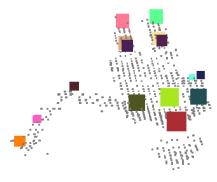
 casts a 3D vote (orange line) for each joint.")
9 TRANS. PAMI, SUBMITTED FOR REVIEW, input image input image front view front view votes top clustered hypothesis votes top clustered hypothesis occluded l. shoulder top view occluded r. knee top view Fig. 7. Offset joint regression voting at test time. Each pixel (black square) casts a 3D vote (orange line) for each joint. Mean shift is used to aggregate these votes and produce a final set of 3D predictions for each joint. The highest confidence prediction for each joint is shown. Note accurate prediction of internal body joints even when occluded. a tracking algorithm to self-initialize and recover from failure. A simple option might be to accumulate the global centroid of the votes for each joint. However, the votes are typically highly multi-modal, and so such a global estimate is inappropriate. Instead we employ a local mode finding approach based on mean shift [55]. We first define a Gaussian Parzen density estimator per joint j as p m j (x ) x w exp x 2 b m, (6) j (x,w) X m j where x is a coordinate in 3D world space, m {BPC, OJR} indicates the approach, and b m j is a learned per-joint bandwidth. Mean shift is then used to find modes in this density m efficiently. The algorithm starts at a subset ˆX j Xj m of the votes, and iteratively walks up the density by computing the mean shift vector [55] until convergence. Votes that converge to the same 3D position within some tolerance are grouped together, and each group forms a body joint proposal, the final output of our system. A confidence weight is assigned to each proposal as the sum of the weights w of the votes in the corresponding group. For both BPC and OJR this proved considerably more reliable than taking the modal density estimate (i.e. the value p j (x BPC )). For BPC the starting point subset ˆX j is defined as all votes for which the original body part probability was above a learned probability threshold α c(j). For OJR, all votes are used as starting points, i.e. ˆX OJR j = X OJR j. 3.5 Training Each tree in the decision forest is trained on a set of images randomly synthesized using the method described in Sec. 2. Because we can synthesize training data cheaply, we use a different set of training images for each tree in the forest. As described above, each image is fully labeled: for BPC there is one body part label c per foreground pixel u, and for OJR there is instead one pose P = (p 1,..., p J ) of 3D joint position vectors p j per training image. For notational simplicity, we will assume that u uniquely encodes a 2D pixel location in a particular image, and thus can range across all pixels in all training images. A random subset of N ex = 2000 example pixels from each image is used. Using a subset of pixels reduces training time and ensures a roughly even contribution from each training image. The following sections describe training the structure of the trees, the leaf node prediction models, and the hyper-parameters. Note that we can decouple the training of the tree structure from the training of the leaf predictors; more details are given below Tree structure training To train the tree structure, and thereby the weak learner parameters used at the split nodes, we use the standard greedy decision tree training algorithm. At each node, a set T of many candidate weak learner parameters θ T is sampled (these θ parameters are those used in Eq. 4). Each candidate is then evaluated against an objective function I. Each sampled θ induces a partition of the set S = {u} of all training pixels that reached the node, into left S L (θ) and right S R (θ) subsets, according to the evaluation of the weak learner function (Eq. 4). The best θ is selected according to θ = argmin θ T d {L,R} S d (θ) I(S d (θ)) (7) S which minimizes objective function I while balancing the sizes of the left and right partitions. We investigate both classification and regression objective functions, as described below. If the tree is not too deep, the algorithm then recurses on the example sets S L (θ ) and S R (θ ) for the left and right child nodes respectively. Training the tree structure is by far the most expensive part of the training process, since many candidate parameters must be tried at an exponentially growing


 Uniform (b) Mixture Offset Proposals Selected Offsets I cls (S) = c p(c S) log p(c S), (8) where p(c S) is the normalized histogram of the set of body part labels c(u) for")
10 Offset Proposal Distribut TRANS. PAMI, SUBMITTED FOR REVIEW, number of tree nodes as the depth increases. To keep the training times practical we employ a distributed implementation. At the high end of our experiments, training 3 trees to depth 20 from 1 million images takes about a day on a 1000 core cluster. (GPU based implementations are also possible and might be considerably cheaper). The resulting trees each have roughly 500K nodes, suggesting fairly balanced trees. We next describe the two objective functions investigated in this work. Classification. The standard classification objective I cls (S) minimizes the Shannon entropy of the distribution of the known ground truth labels corresponding to the pixels in S. Entropy is computed as (a) Uniform (b) Mixture Offset Proposals Selected Offsets I cls (S) = c p(c S) log p(c S), (8) where p(c S) is the normalized histogram of the set of body part labels c(u) for all u S. Regression. Here, the objective is to partition the examples to give nodes with minimal uncertainty in the joint offset distributions at the leaves [56], [20]. In our problem, the offset distribution for a given tree node is likely to be highly multi-modal (see examples in Fig. 9). One approach might be to fit a Gaussian mixture model (GMM) to the offsets and use the negative log likelihood of the offsets under this model as the objective. However, GMM fitting would need to be repeated at each node for thousands of candidate weak learners, making this prohibitively expensive. Another possibility might be to use non-parametric entropy estimation [57], but again this would increase the cost of training considerably. Following existing work [20], we instead employ the much cheaper sum-of-squared-differences objective: I reg (S) = u j µ j 2 2, (9) j u S j where offset vector u j = p j x(u), and 1 µ j = u j, (10) S j u S j S j = { u S u j 2 < ρ }. (11) Unlike [20], we introduce an offset vector length threshold ρ to remove offsets that are large and thus likely to be outliers (results in Sec highlight importance of ρ). While this model implicitly assumes a uni-modal Gaussian, which we know to be unrealistic, for learning the tree structure, this assumption is tractable and can still produce satisfactory results. Discussion. Recall that the two objective functions above are used for training the tree structure. We are then at liberty to fit the leaf prediction models in a different fashion (see next section). Perhaps counter-intuitively, we observed in our experiments that optimizing with the classification objective I cls works well for the OJR task. Training for classification will result in image patches reaching the leaf nodes that tend to have both similar Fig. 8. Sampling strategies for δ. (a) A uniform proposal distribution is used to sample the 2D feature offsets δ (see Eq. 3) during tree structure training. After training, a 2D histogram of the selected δ values across all split nodes in the forest is plotted. The resulting distribution is far from uniform. (b) Building a mixture distribution to approximate these selected offsets, the tree structure training selects a similar distribution of offsets. However, as seen in Fig. 11(e,f), this can have a substantial impact on training efficiency. appearances and local body joint configurations. This means that for nearby joints, the leaf node offsets are likely to be small and tightly clustered. The classification objective further avoids the assumption of the offset vectors being Gaussian distributed. We did investigate further node splitting objectives, including various forms of mixing body part classification and regression (as used in [20]), as well as variants such as separate regression forests for each joint. However, none proved better than either the standard classification or regression objectives defined above. Sampling θ. The mechanism for proposing T, the set of candidate weak learner parameters θ, merits further discussion, especially as the search space of all possible θ is large. The simplest strategy is to sample T values of θ from a uniform proposal distribution p(θ), defined here over some range of offsets φ = (δ 1, δ 2 ) and over some range of thresholds τ. If the forest is trained using this proposal distribution, one finds that the empirical distribution p(θ ) (computed over the chosen θ across all nodes in the forest) ends up far from uniform. This suggests an iterative strategy: start from a uniform proposal distribution p(θ), train the forest, examine the distribution p(θ ) of the chosen θ s, design an improved non-uniform proposal distribution p (θ) that approximates p(θ ), and repeat. The intuition is that if you show the training algorithm more features that are likely to be picked, it will not need to see so many to find a good one. To make this procedure safe the new proposal distribution p (θ) can include a mixture with
11 TRANS. PAMI, SUBMITTED FOR REVIEW, a uniform distribution with a small mixture coefficient (e.g. 10%). In practice we observed a small but consistent improvement in accuracy when iterating this process once (see Fig. 11(e,f)), though further iterations did not help. See Fig. 8 for an illustration. This idea is explored further in [58] Leaf node prediction models Given the learned tree structure, we must now train the prediction models at the leaf nodes. It is possible to first train the tree structure as described in the previous section, and then retro-fit the leaf predictors by passing all the training examples down the trained tree to find the set of training examples that reach each individual leaf node. This allows us to investigate the use of different tree structure objectives for a given type of prediction model; see results below in Sec For the BPC task, we simply take p l (c) = p(c S), the normalized histogram of the set of body part labels c(u) for all pixels u S that reached leaf node l. For OJR, we must instead build the weighted relative vote sets V lj = {( ljk, w ljk )} K k=1 for each leaf and joint. To do this, we employ a clustering step using mean shift, detailed in Algorithm 3. This algorithm describes how each training pixel induces a relative offset to all ground truth joint positions 2, and once aggregated across all training images, these are clustered using mean shift. To maintain practical training times and keep memory consumption reasonable we use reservoir sampling [59] to sample N res offsets. Reservoir sampling is an algorithm that allows one to maintain a fixed-size unbiased sample from a potentially infinite stream of incoming samples; see [59] for more details. In our case, it allows us to uniformly sample N res offsets at each node from which to learn the prediction models, without having to store the much larger set of offsets being seen. Mean shift mode detection is again used for clustering, 2. Recall that for notational simplicity we are assuming u defines a pixel in a particular image; the ground truth joint positions P used will therefore correspond for each particular image. Algorithm 3 Learning relative votes 1: // Collect relative offsets 2: initialize R lj = for all leaf nodes l and joints j 3: for all training pixels u S do 4: descend tree to reach leaf node l = l(u) 5: compute 3D pixel position x(u) 6: for all joints j do 7: lookup ground truth joint positions P = {p j} 8: compute relative offset u j = p j x(u) 9: store u j in R lj with reservoir sampling 10: // Cluster 11: for all leaf nodes l and joints j do 12: cluster offsets R lj using mean shift 13: discard modes for which ljk 2 > threshold λ j 14: take top K weighted modes as V lj 15: return relative votes V lj for all nodes and joints this time on the following density: p lj ( ) ( 2) b. (12) R lj exp This is similar to Eq. 6, though now defined over relative offsets, without weighting, and using a learned bandwidth b. Fig. 9 visualizes a few examples sets R lj that are clustered. The positions of the modes form the relative votes ljk and the numbers of offsets that reached each mode form the vote weights w ljk. To prune out long range predictions which are unlikely to be reliable, only those relative votes that fulfil a per joint distance threshold λ j are stored; this threshold could equivalently be applied at test time though would waste memory in the tree. In Sec , we show that there is little or no benefit in storing more than K = 2 relative votes per leaf. We discuss the effect of varying the reservoir capacity in Sec In our unoptimized implementation, learning these relative votes for 16 joints in 3 trees trained with 10K images took approximately 45 minutes on a single 8-core machine. The vast majority of that time is spent traversing the tree; the use of reservoir sampling ensures the time spent running mean shift totals only about 2 minutes Learning the hyper-parameters Some of the hyper-parameters used in our methods are the focus of our experiments below in Sec. 4.4 and Sec Others are optimized by grid search to maximize our mean average precision over a 5K image validation set. These parameters include the probability thresholds α c (the chosen values were between 0.05 and 0.3), the surface push-backs ζ j (between 0.013m to 0.08m), the test-time aggregation bandwidths b m j (between 0.03m and 0.1m), the shared training-time bandwidth b (0.05m). 4 EXPERIMENTS In this section we describe the experiments performed to evaluate our method on several challenging datasets. We begin by describing the test data sets and error metrics, before giving some qualitative results. Following that, we examine in detail the effect of various hyperparameters on BPC and then OJR. We finally compare the two methods, both to each other and to alternative approaches. 4.1 Test data We use both synthetic and real depth images to evaluate our approach. For the synthetic test set ( MSRC-5000 ), we synthesize 5000 test depth images, together with the ground truth body part labels and body joint positions, using the pipeline described in Sec. 2. However, to ensure a fair and distinct test set, the original mocap poses used to generate these test images are held out


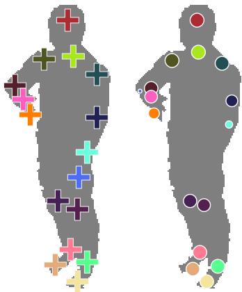


12 TRANS. PAMI, SUBMITTED FOR REVIEW, 2012 left shoulder joint 12 left elbow joint left hand joint right knee joint OJR silhouette results offset joint regression body part classification Fig. 9. Empirical offset distributions for offset joint regression. We visualize the set Rlj of 3D relative offset vectors u j. Each set of axis represents a different leaf node, and the orange squares plot the vectors u j Rlj at that leaf. (The red, green, and blue squares indicate respectively the positive x, y, and z axes; each half-axis represents 0.5m in world space). We also show training images for each node illustrating the pixel that reached the leaf node as a cyan cross, and the offset vector as an orange arrow. Note how the decision trees tend to cluster pixels with similar local appearance at the leaves, but the inherent remaining ambiguity results in multi-modal offset distributions. The OJR algorithm compresses these distributions to a very small number of modes while maintaining high test accuracy. Fig. 10. Example inferences on both synthetic and real test images. In each example we see the input depth image, the inferred most likely body part labels (for BPC only), and the inferred body joint proposals shown as front, right, and top views overlaid on a depth point cloud. Only the most confident proposal for each joint above a fixed, shared threshold is shown, though the algorithms predict multiple proposals per joint. Both algorithms achieve accurate prediction of body joints for varied body sizes, poses, and clothing. We show failure modes in the bottom rows of the two larger panels. There is little qualitatively to tell between the two algorithms, though the middle row of the OJR results shows accurate prediction of even occluded joints (not possible with BPC), and further results in Sec. 4.6 compare quantitatively. Best viewed digitally at high zoom.
13 TRANS. PAMI, SUBMITTED FOR REVIEW, from the training data. Our real test set consists of 8808 frames of real depth images over 15 different subjects, hand-labeled with dense body parts and 7 upper body joint positions. We also evaluate on the real test depth data from [6]. As we will see, the results are highly correlated between the synthetic and real data. Furthermore, our synthetic test set appears to be far harder than either of the real test sets due to its extreme variability in pose and body shape. After some initial experiments we thus focus our evaluation on the harder synthetic test set. In most of the experiments below, we limit the rotation of the user to ±120 in both training and synthetic test data since the user is facing the camera (0 ) in our main entertainment scenario. However, we do also investigate the full 360 scenario. 4.2 Error metrics We quantify accuracy using (i) a classification metric (for BPC only) and (ii) a joint prediction metric (for both BPC and OJR). As the classification metric, we report the average per-class segmentation accuracy. This metric is computed as the mean of the diagonal elements of the confusion matrix between the ground truth body part label and the most likely inferred label. This metric weights each body part equally despite their varying sizes. As the joint prediction metric, we generate recallprecision curves as a function of the predicted confidence threshold, as follows. All proposals below a given confidence threshold are first discarded; varying this threshold gives rise to the full recall-precision curve. Then, the first body joint proposal within a threshold D tp meters of the ground truth position is taken as a true positive, while any other proposals that are also within D tp meters count as false positives. This penalizes multiple spurious detections near the correct position which might slow a downstream tracking algorithm. Any proposals outside D tp meters also count as false positives. Any joint for which there is no proposal of sufficient confidence within D tp is counted as a false negative. However, we choose not to penalize joints that are invisible in the image as false negatives. Given the full recall-precision curve, we finally quantify accuracy as average precision (the area under the curve) per joint, or mean average precision (map) over all joints. Note that, for example, a mean squared error (MSE) metric is inappropriate to evaluate our approach. Our algorithms aim to provide a strong signal to initialize and re-initialize a subsequent tracking algorithm. As such, evaluating our approach on MSE would fail to measure joints for which there are zero or more than one proposal, and would fail to measure how reliable the joint proposal confidence measures are. Our map metric effectively measures all proposals (not just the most confident): the only way to achieve a perfect score of 1 is to predict exactly one proposal for each joint that lies within D tp of the ground truth position. For most results below we set D tp = 0.1m as the threshold, though we investigate the effect of this threshold below in Fig. 14c. For BPC we observe a strong correlation of classification and joint prediction accuracy (cf. the blue curves in Fig. 11(a) and Fig. 15(b)). This suggests the trends observed below for one also apply for the other. For brevity we thus present results below for only the more interesting combinations of methods and metrics. 4.3 Qualitative results Fig. 10 shows example inferences for both the BPC and OJR algorithms. Note high accuracy of both classification and joint prediction, across large variations in body and camera pose, depth in scene, cropping, and body size and shape (e.g. small child vs. heavy adult). Note that no temporal or kinematic constraints (other than those implicitly encoded in the training data) are used for any of our results. When tested on video sequences (not shown), most joints can be accurately predicted in most frames with remarkably little jitter. A few failure modes are evident: (i) difficulty in distinguishing subtle changes in depth such as the crossed arms; (ii) for BPC, the most likely inferred part may be incorrect, although often there is still sufficient correct probability mass in distribution p(c u) that an accurate proposal can still result during clustering; and (iii) failure to generalize well to poses not present in training. However, the inferred confidence values can be used to gate bad proposals, maintaining high precision at the expense of recall. In these and other results below, unless otherwise specified, the following training parameters were used. We trained 3 trees in the forest. Each was trained to depth 20, on 300K images per tree, using N ex = 2000 training example pixels per image. At each node we tested 2000 candidate offset pairs φ and 50 candidate thresholds τ per offset pair, i.e. T = Below, unless specified, the number of images used refers to the total number used by the whole forest; each tree will be trained on a subset of these images. 4.4 Body part classification (BPC) experiments We now investigate the effect of several training parameters on the BPC algorithm, using the classification accuracy metric. The following sections refer to Fig Number of training images In Fig. 11(a) we show how test accuracy increases approximately logarithmically with the number of randomly generated training images, though starts to tail off around 100K images. This saturation could be for several reasons: (i) the model capacity of the tree has been reached; (ii) the error metric does not accurately capture the continued improvement in this portion of the graph (e.g. the underlying probability distribution is

 (b) (c) 35% 30% 0 100 200 300 Maximum probe offset (pixel meters) 1 tree 3 trees 54% 54% 55% 52% 52% 50% 50% 50% 48% 48% 46% 46% 45% Synthetic test set Real test set 40% 1")
 (e) (f) 44% 42% 40% Real test, Uniform Real test, Mixture Synthetic test, Uniform Synthetic test, Mixture 0 10 20 30 40 50 Number of candidate thresholds τ Fig. 11. Training parameters vs.")
 Number of candidate features φ and thresholds τ evaluated during training, for both real and synthetic test data, and using a uniform and mixture proposal distribution during tree structure")
14 Average per-class accuracy Average per-class accuracy Average per-class accuracy Average per-class accuracy Average per-class accuracy Average per-class accuracy Combined Results TRANS. PAMI, SUBMITTED FOR REVIEW, % 50% 60% 55% Synthetic Test Set 60% 55% Real Test Set 60% 55% Real test data Synthetic test data 40% 50% 50% 50% 45% 45% 45% 30% 40% 40% 40% 20% Synthetic test set Real test set 10% % 35% 900k training images 900k training images 30% 15k training images 30% 15k training images Depth of trees Depth of trees 20 (a) Num. training images (log scale) (b) (c) 35% 30% Maximum probe offset (pixel meters) 1 tree 3 trees 54% 54% 55% 52% 52% 50% 50% 50% 48% 48% 46% 46% 45% Synthetic test set Real test set 40% Number of trees 6 trees ground truth 44% Real test, Uniform Real test, Mixture 42% Synthetic test, Uniform Synthetic test, Mixture 40% Number of candidate features φ (d) (e) (f) 44% 42% 40% Real test, Uniform Real test, Mixture Synthetic test, Uniform Synthetic test, Mixture Number of candidate thresholds τ Fig. 11. Training parameters vs. classification accuracy of the body part classification (BPC) algorithm. (a) Number of training images. (b) Depth of trees. (c) Maximum depth probe offset. (d) Number of trees. (e,f) Number of candidate features φ and thresholds τ evaluated during training, for both real and synthetic test data, and using a uniform and mixture proposal distribution during tree structure training (see Sec ). improving but the MAP label is constant); or (iii) the training images are rendered using a fixed set of only 100K poses from motion capture (though with randomly chosen body shapes, global rotations and translations). Given the following result, the first of these possibilities is quite likely Depth of trees Fig. 11(b) shows how the depth of trees affects test accuracy using either 15K or 900K images. Of all the training parameters, depth appears to have the most significant effect as it directly impacts the model capacity of the classifier. Using only 15K images we observe overfitting beginning around depth 17, but the enlarged 900K training set avoids this. The high accuracy gradient at depth 20 suggests even better results can be achieved by training still deeper trees, at a small extra run-time computational cost and a large extra memory penalty Maximum probe offset The range of depth probe offsets φ allowed during training has a large effect on accuracy. We show this in Fig. 11(c) for 5K training images, where maximum probe offset means the maximum absolute value proposed for both x and y coordinates of δ 1 and δ 2 in Eq. 3. The concentric boxes on the right show the five tested maximum offsets, calibrated for a left shoulder pixel in that image (recall that the offsets scale with the world depth of the pixel). The largest maximum offset tested covers almost all the body. As the maximum probe offset is increased, the classifier is able to use more spatial context to make its decisions. (Of course, because the search space of features is enlarged, one may need a larger set T of candidate features during training). Accuracy increases with the maximum probe offset, though levels off around 129 pixel meters, perhaps because a larger context makes overfitting more likely Number of trees We show in Fig. 11(d) test accuracy as the number of trees is increased, using 5K images for each depth 18 tree. The improvement starts to saturate around 4 or 5 trees, and is considerably less pronounced than when making the trees deeper. The error bars give an indication of the remarkably small variability between trees. The qualitative results illustrate that more trees tend to reduce noise, though even a single tree can get the overall structure fairly well Number of features and thresholds Fig. 11(e,f) shows the effect of the number of candidate features φ and thresholds τ evaluated during tree training. Using the mixture proposal distributions for sampling φ and τ (see Sec ) allows for potentially
15 Head Neck L. Shoulder R. Shoulder L. Elbow R. Elbow L. Wrist R. Wrist L. Hand R. Hand L. Knee R. Knee L. Ankle R. Ankle L. Foot R. Foot Mean AP Average precision TRANS. PAMI, SUBMITTED FOR REVIEW, OJR forest with tree structure trained using objectives: Classification Regression I reg I cls (ρ = 0.3m) Regression I reg (ρ = ) Fig. 12. Comparison of tree structure objectives used to train the offset joint regression forest. In all cases, after the tree structure has been trained, the same regression model is fit for each leaf node, as described in Sec much higher training efficiency. Most of the gain occurs up to 500 features and 20 thresholds per feature. On the easier real test set the effects are less pronounced. These results used 5K images for each of 3 trees to depth 18. The slight peaks on the mixture proposal curves are likely down to overfitting Discussion The trends observed above on the synthetic and real test sets appear highly correlated. The real test set appears consistently easier than the synthetic test set, probably due to the less varied poses present. For the remaining experiments, we thus use the harder synthetic test set. We now switch our attention to the joint prediction accuracy metric. We have observed (for example, cf. the blue curves in Fig. 11(a) and Fig. 15(b)) a strong correlation between the classification and joint prediction metrics. We therefore expect that the trends observed above also apply to joint prediction. 4.5 Offset joint recognition (OJR) experiments The previous section investigated the effect of many of the system parameters for BPC. We now turn to the OJR algorithm and perform a similar set of experiments. The results in this section all make use of the average precision metric on joint prediction accuracy (see Sec. 4.2) Tree structure objectives The task of predicting continuous joint locations from depth pixels is fundamentally a regression problem. Intuitively, we might expect a regression-style objective function to produce the best trees for our approach. To investigate if this is indeed the case, we evaluated several objective functions for training the structure of the decision trees, using forests trained with 5K images. The results, comparing average precision on all joints, are summarized in Fig. 12. Surprisingly, for all joints except head, neck, and shoulders, trees trained using the classification objective I cls (i.e. training the tree structure for BPC using Eq. 8, but then retro-fitting the leaf prediction models for OJR; see Sec ) gave the highest accuracy. We believe the uni-modal assumption implicit in the regression objective (Eq. 9) may be causing this, and that classification of body parts is a reasonable proxy for a regression objective that correctly accounts for multi-modality. A further observation from Fig. 12 is that the ρ threshold parameter (used in Eq. 11 to remove outliers) does improve the regression objective, but not enough to beat the classification objective. Another possible problem with Eq. 9 could be the summation over joints j. To investigate this, we experimented with training separate regression forests, each tasked with predicting the location of just a single joint. A full forest was trained with 5K images for each of four representative joints: head, l. elbow, l. wrist, and l. hand. With ρ =, they achieved AP scores of 0.95, 0.564, 0.508, and respectively (cf. the green bars in Fig. 12: 0.923, 0.403, 0.359, and respectively). As expected, due to greater model capacity (i.e. one forest for each joint vs. one forest shared for all joints), the per-joint forests produce better results. However, these results are still considerably worse than the regression forests trained with the classification objective. Given these findings, the following experiments all use the classification objective Tree depth and number of trees Fig. 13(a) shows that mean average precision (map) rapidly improves as the tree depth increases, though it starts to level off around depth 18. As with BPC, the tree depth is much more important than the number of trees in the forest: with just one tree, we obtain a map of 0.730, with two trees 0.759, and with three trees Vote length threshold We obtain our best results when using a separate voting length threshold λ j for each joint (see Algorithm 3). These thresholds are optimized by grid search on a 5K validation data set, using a step size of 0.05m in the range [0.05, 0.60]m. In Fig. 13(b) we compare accuracy obtained using a single learned threshold shared by all joints (the blue curve), against the map obtained with per-joint thresholds (the dashed red line). When using a shared threshold it appears critical to include votes from pixels at least 10cm away from the target joints. This is likely because the joints are typically over 10cm away from the surface where the pixels lie. We next investigate the effect of the metric used to optimize these thresholds. Interestingly, the optimized length thresholds λ j turn out quite differently, according to whether the failure to predict an occluded joint is counted as a false negative or simply ignored. In Table 1, we see that longer range votes are chosen to maximize map when the model is penalized for missing occluded joints. In some cases, such as head, feet, and ankles, the difference is quite large. This makes sense: occluded
16 Mean average precision Mean average precision Mean average precision TRANS. PAMI, SUBMITTED FOR REVIEW, Tree depth shared threshold threshold tuned per joint Offset vote length threshold (m) (a) (b) (c) Body part classification Body part classification (approx.) Offset joint regression Frames per second Fig. 13. Effect of various system parameters on the offset joint regression (OJR) algorithm. (a) map vs. tree depth. (b) map vs. a single, shared vote length threshold for all joints. (c) map vs. fps. The blue curve is generated by varying N sub, the number of votes retained before running mean shift at test time joints tend to be further away from visible depth pixels than non-occluded joints, and predicting them will thus require longer range votes. This experiment used 30K training images Number of votes per leaf K Increasing K, the maximum number of votes stored at each leaf, from 1 to 2 boosted map slightly from to However, for K [2, 10] there was no appreciable difference in accuracy, and so for all other experiments presented we used K = 2. We hypothesize that aggregating over many image pixels that reach a diverse set of leaf nodes makes storing multiple local modes in each leaf node somewhat redundant. The comparison in Sec illustrates how accuracy may change as K gets much larger Using mean offsets We tried using a single relative vote lj1 chosen to be the mean of the offsets reaching each leaf for each joint, rather than the top local mode. (Note that our model errors on occluded joints: not penalized penalized λ j λ j Head Neck L. Shoulder R. Shoulder L. Elbow R. Elbow L. Wrist R. Wrist L. Hand R. Hand L. Knee R. Knee L. Ankle R. Ankle L. Foot R. Foot TABLE 1 Optimized values for the test-time vote length thresholds λ j under two different error metrics. learned using mean shift with K = 1 is not the same as taking the mean of all the data). To achieve a sensible result, we found the mean vote s weight w ij1 to be very important. The best result obtained took w ij1 as the number of offsets within 5cm of the mean. Performance decreased from (top local mode with K = 1) to (mean of all offsets). Significant degradation was observed in the arm joints which exhibit much more multi-modality in the offsets: computed over elbows, wrists, and hands, the map dropped from to For robust results, using the top local mode thus appears better than the mean Learned relative vote weights w ljk To quantify the role of the relative vote weights, we tested our system with w ljk = 1, l, j, k. This uniform weight assignment decreased map dramatically from to 0.542, underscoring the importance of learning the vote weights Training-time reservoir capacity N res The size of the reservoir had relatively little effect on accuracy. Reducing the reservoir capacity from 100 to 50 led to a small decrease in accuracy from map to Interestingly, increasing the reservoir capacity to 200 and 300 also caused a small drop (0.755 and 0.747, respectively). These results suggest that even a small sample of offsets is sufficient to characterize their distribution well for clustering Test-time vote sub-sampling N sub Even with the learned vote length thresholds λ j, an average of about 1000 votes are cast per joint when processing a test image. As described in Algorithm 2, prior to aggregating votes with mean shift, we optionally sub-sample the voting space to at most N sub votes. First, using fixed N sub = 200, we experimented with different sub-sampling strategies: top N sub weighted votes; uniformly random sampling; random sampling weighted by vote weight. These three methods achieved map scores of 0.770, 0.727, and 0.753, respectively. Second, using the top N sub strategy, we found that accuracy varies slowly with N sub. We illustrate the substantial improvement in runtime speed this allows in
17 Head Neck L. Shoulder R. Shoulder L. Elbow R. Elbow L. Wrist R. Wrist L. Hand R. Hand L. Knee R. Knee L. Ankle R. Ankle L. Foot R. Foot Mean AP Mean average precision Average precision Mean average precision TRANS. PAMI, SUBMITTED FOR REVIEW, (a) Body part classification Offset joint regression Total number of training images (in thousands) (b) Body part classification Offset joint regression Body part classification 0.1 Offset joint regression True positive distance threshold (c) D tp (m) Fig. 14. Comparing body part classification (BPC) with offset joint regression (OJR). (a) Effect of total number of training images. The dashed line shows the best result of BPC trained with 900K images. (b) Average precision on each of the 16 test body joints. (c) Effect of the true positive threshold D tp on the metric. Fig. 13(c). This graph plots map against fps as a function of N sub, and compares with the BPC algorithm (and BPC running an approximate but faster implementation). Representative values of N sub from 1 to 400 are overlaid on the plot. The best tradeoff between prediction accuracy and prediction speed is at about N sub = 50. All timings were measured on an 8-core machine taking advantage of CPU parallelism. Using sub-sampling to achieve speedups, while maintaining acuracy, is only possible if the vote weights are well correlated with predictive strength, further underscoring the importance of vote weight learning. 4.6 Comparison between BPC and OJR Having investigated the BPC and OJR algorithms separately above, we now compare these algorithms to each other. Fig. 14(a) compares mean average precision for different training set sizes. In all cases we observe OJR performing more accurately than BPC. In Fig. 14(b) we show a per-joint breakdown of these results, using the best results obtained for each method (900K and 300K training images for BPC and OJR respectively). 3 There are several possible reasons for OJR giving a more accurate result than BPC. One possibility is that OJR can directly regress the positions of joints inside the body. The joints showing the most substantial improvements (head, neck, shoulders, and knees) are also those where surface body parts cover a large area and are furthest from the joint center. Another ability of OJR is predicting occluded joints. When the map metric is changed to penalize failure to predict occluded joints, the improvement of OJR over BPC is even more apparent: vs (both methods trained with 30K images). Example inferences showing localization of occluded joints are presented in Fig. 10 (OJR panel, middle row). As previously observed in Fig. 13(c), the OJR algorithm can also make predictions faster than BPC. 3. The results for OJR at 300K images were already better than the equivalent BPC forest trained with 900K images (see Fig. 14a), and so we chose not to expend the considerable energy in training a directly comparable 900K forest True positive threshold A value of D tp = 0.1m is used as the true positive radius for most of the results presented here. We quantify the effect of this threshold on the map score in Fig. 14(c). The OJR algorithm maintains considerably higher map score as the radius shrinks in comparison to BPC Full rotations To evaluate the scenario of full 360 rotation of the user, we trained BPC and OJR forests on images containing full rotations, and tested on 5K synthetic full rotation images. Despite the massive increase in left-right ambiguity, both approaches do remarkably well. Trained on 900K images, the BPC forest achieved an map of 0.655, while, trained on 300K images, the OJR forest achieved an map of These results indicate that the forests can accurately learn the subtle visual cues that distinguish front and back facing poses. The residual left-right ambiguity might be handled by a tracking algorithm that propagates multiple hypotheses through time Multiple people Our approach can propose joint positions for multiple people in the image: neither the forest evaluation at each pixel nor the aggregation step are limited to a single person. The forest could be explicitly trained with images containing multiple people, but in practice generalizes well without such explicit training. Preliminary results of this are given in the supplementary video Silhouette images Although we focus on depth images in this paper, our methods can be applied without modification to 2D silhouette images. Silhouettes might readily be obtained using color segmentation or static background subtraction from RGB images. To prototype this scenario, we flattened both the training and test images to a fixed canonical depth, 2m, producing silhouettes in which the body size is unknown. To compute average precision for this 2D prediction task, we modified the true positive
18 Head Neck L. Shoulder R. Shoulder L. Elbow R. Elbow L. Wrist R. Wrist L. Hand R. Hand L. Knee R. Knee L. Ankle R. Ankle L. Foot R. Foot Mean AP Average precision Mean average precision TRANS. PAMI, SUBMITTED FOR REVIEW, (a) Ganapathi et al. (tracking) Body part classification (per frame) Offset joint regression (per frame) 0.8 Body part classification 0.7 Oracle NN skeleton 0.6 Chamfer NN Number of training images (log scale) (b) Fig. 15. Comparisons to the state of the art. (a) Comparison with [6]. Even without the kinematic and temporal constraints exploited by [6], both our approaches are able to more accurately localize body joints. (b) Comparison between BPC and nearest neighbor matching. Example chamfer matches shown right. radius to an absolute pixel distance, ˆDtp = 10 pixels. BPC achieves map, and OJR achieves map. Example inferences of OJR from silhouettes appear in the bottom right panel of Fig. 10, where the crosses show the ground truth, and the circles show the inferred joint predictions. Note how the proposal confidences (shown as the circle radii) correlate well with the ambiguity in the signal. The most probable reason for the significant drop in accuracy is due to missing information. For example, whenever a hand crosses in front of the body, the silhouettes will likely not contain enough information to reliably detect the hand. 4.7 Comparison to the state of the art In this final evaluation section, we compare our algorithms to other methods Comparison to Ganapathi et al. [6] The authors of [6] kindly provided their test data and results for direct comparison. Their algorithm uses sparse body part proposals from [5] and further tracks the skeleton with kinematic and temporal information. Their real data comes from a time-of-flight depth camera with very different noise characteristics to our structured light sensor. Without any changes to our training data or algorithm, Fig. 15(a) shows considerably improved joint prediction average precision for both BPC and OJR. Our algorithms also run at least 10 times faster, though we do of course require the large training corpus Whole pose nearest neighbor matching Both of our methods attempt to find the body joints independently of each other. One alternative is to attempt to match a whole pose at once. Whole pose matching has the benefit of an extremely informative raw signal, but unfortunately has a search space that is exponential in the number of articulated joints. We compare our BPC algorithm with two variants of whole pose matching in Fig. 15(b). The first, idealized, variant matches the ground truth test skeleton to a set of training exemplar skeletons with optimal rigid translational alignment in 3D world space. Of course, in practice one has no access to the test skeleton. While this oracle is thus not an achievable algorithm, it does give us an upper bound on whole pose matching accuracy. As an example of a realizable system, the second variant uses chamfer matching [60] to compare the test image to the training exemplars. This is computed using depth edges and 12 orientation bins. To make the chamfer task easier, we throw out any cropped training or test images. We align images using the 3D center of mass, and found that further local rigid translation only reduced accuracy. Our BPC algorithm, recognizing in parts, generalizes better than even the idealized skeleton matching until about 150K training images are reached. The speed of nearest neighbor chamfer matching is also drastically slower (2 fps) than our algorithm. While hierarchical matching [60] might be faster, one would still need a massive exemplar set to achieve comparable accuracy Comparison between OJR and Hough forests [20] We compare OJR and Hough forests [20], using an identical tree structure for both. There are two main algorithmic differences. First, OJR clusters the offsets during training. This contrasts with Hough forests where all offset vectors are stored. To compare, we re-train the leaf nodes of our OJR forest, storing up to 400 offset votes for each joint, uniformly sampled (using all votes would have been prohibitive). The second difference is that we use a continuous voting space at test time, while Hough forests instead discretize the voting volume. Unfortunately, the inherent 3D nature of our problem makes discrete voting much less attractive than for 2D prediction. Our test data covers a large voting volume of 4m 4m 5m. To allow accurate localization we used a voxel resolution of 2cm per side, resulting in a voting volume with 10 million bins. At test time, we smooth the voting volume using a Gaussian of fixed standard deviation 1.3cm. Due to memory and runtime constraints we compare on two representative joints (an easy joint, head, and a hard joint, left hand) in Fig. 16. Interestingly, even with discrete voting, using two votes per leaf performs
19 Average precision TRANS. PAMI, SUBMITTED FOR REVIEW, slightly better than voting with a large number of stored offsets. This is likely due to the clustering removing many outliers making the final density much peakier. The results also show the clear improvement obtained by using the classification objective to train the tree structure instead of the regression objective as used in [20]. (This reiterates the findings from Fig. 12). Our implementation of the Hough voting ran at approximately 0.5 fps for only 2 body joints, compared to around 200 fps for OJR which predicts all 16 joints. We experimented with a few voxel resolutions and smoothing kernel sizes, though the slow runtime speed prohibited selection of per joint smoothing kernel widths by grid search. 5 CONCLUSIONS We have presented two algorithms, body part classification and offset joint regression. The two algorithms have much in common. They both use decision forests and simple depth-invariant image features. Both methods exploit a large, highly varied, synthetic training set, allowing us to train very deep trees. We have shown that the forests can learn invariance to both pose and shape while avoiding overfitting. The BPC approach introduces a set of surface body parts that the forest tries to infer. These body parts are aligned with the joints of interest, so that an accurate classification will localize the joints of the body. The OJR approach instead casts votes that try to directly predict the positions of interior body joints. In both methods, mean shift is used to aggregate votes to produce a final set of confidence-weighted 3D body joint proposals. Our experiments have demonstrated that both algorithms can accurately predict the 3D locations of body joints in super-realtime from single depth or silhouette images. We have further shown state of the art accuracy and speed against several competing approaches. The body joint proposals might be used as an output in their own right, or used for initialization and re-initialization of a subsequent tracking and model fitting algorithm that exploits temporal and kinematic constraints. Of our two approaches, which should you use? The numerical results show that OJR will give considerably higher accuracy than BPC. OJR also seems intuitively a cleaner solution: it does not need the intermediate definition of body parts, and the offsets vote directly for interior joint positions. This also means that OJR is capable of predicting occluded joints, while BPC will instead give no proposals for an occluded joint. However, OJR proved considerably more complex: the obvious regression objective does not work well, and many hyperparameters had to be optimized against a validation set. A promising direction for future work is to investigate alternative efficient tree-structure learning objectives that handle multi-modal problems effectively Head L. Hand Offset joint regression (continuous) Discrete; 2 votes per leaf Discrete; max 400 votes per leaf Tree objective: I cls Discrete; max 400 votes per leaf Tree objective: I reg (ρ = 0.3m) Fig. 16. Comparison with Hough forest voting [20]. The Hough forest regression objective performs poorly for articulated joint such as hands. Vote compression and continuous voting improve accuracy slightly, while running 3200x faster (see text). ACKNOWLEDGMENTS The authors would like to thank the many skilled engineers in Microsoft who built the Kinect tracking system on top of this research. In particular: Robert Craig, Matt Bronder, Craig Peeper, Momin Al-Ghosien, Sam Mann, and Ryan Geiss. We also thank John Winn, Duncan Robertson, Shahram Izadi, Ollie Williams, and Mihai Budiu for all their help and discussions. Finally thanks to Varun Ganapathi and Christian Plagemann for providing their test data. REFERENCES [1] D. Grest, J. Woetzel, and R. Koch, Nonlinear body pose estimation from depth images, in In Proc. DAGM, [2] S. Knoop, S. Vacek, and R. Dillmann, Sensor fusion for 3D human body tracking with an articulated 3D body model, in Proc. ICRA, [3] Y. Zhu and K. Fujimura, Constrained optimization for human pose estimation from depth sequences, in Proc. ACCV, [4] M. Siddiqui and G. Medioni, Human pose estimation from a single view point, real-time range sensor, in CVCG at CVPR, [5] C. Plagemann, V. Ganapathi, D. Koller, and S. Thrun, Real-time identification and localization of body parts from depth images, in Proc. ICRA, [6] V. Ganapathi, C. Plagemann, D. Koller, and S. Thrun, Real time motion capture using a single time-of-flight camera, in Proc. CVPR, [7] Microsoft Corp. Redmond WA, Kinect. [8] C. Bregler and J. Malik, Tracking people with twists and exponential maps, in Proc. CVPR, [9] L. Sigal, S. Bhatia, S. Roth, M. Black, and M. Isard, Tracking loose-limbed people, in Proc. CVPR, [10] R. Wang and J. Popović, Real-time hand-tracking with a color glove, in Proc. ACM SIGGRAPH, [11] M. Brubaker, D. Fleet, and A. Hertzmann, Physics-based person tracking using the anthropomorphic walker, IJCV, [12] T. Sharp, Implementing decision trees and forests on a GPU, in Proc. ECCV, [13] R. Urtasun and T. Darrell, Sparse probabilistic regression for activity-independent human pose inference, in Proc. CVPR, [14] J. Shotton, A. Fitzgibbon, M. Cook, T. Sharp, M. Finocchio, R. Moore, A. Kipman, and A. Blake, Real-time human pose recognition in parts from a single depth image, in Proc. CVPR. IEEE, [15] R. Fergus, P. Perona, and A. Zisserman, Object class recognition by unsupervised scale-invariant learning, in Proc. CVPR, [16] J. Winn and J. Shotton, The layout consistent random field for recognizing and segmenting partially occluded objects, in Proc. CVPR, [17] L. Bourdev and J. Malik, Poselets: Body part detectors trained using 3D human pose annotations, in Proc. ICCV, 2009.
![TRANS. PAMI, SUBMITTED FOR REVIEW, 2012 20 [18] R. Girshick, J. Shotton, P. Kohli, A. Criminisi, and A. Fitzgibbon, Efficient regression of general-activity human poses from depth images, in Proc.](/docs-images/74/71375571/images/20-0.jpg "ICCV, 2011. [19] D. Comaniciu and P. Meer, Mean shift: A robust approach toward feature space analysis, IEEE TPAMI, vol. 24, no. 5, pp. 603 619, 2002. [20] J. Gall and V.")
![Lempitsky, Class-specific Hough forests for object detection, in IEEE Trans. PAMI, 2009. [21] T. Moeslund, A. Hilton, and V.](/docs-images/74/71375571/images/20-1.jpg "Krüger, A survey of advances in vision-based human motion capture and analysis, CVIU, 2006. [22] R. Poppe, Vision-based human motion analysis: An overview, CVIU, vol. 108, 2007. [23] M.")
![Fischler and R. Elschlager, The representation and matching of pictorial structures, IEEE Trans. on Computers, vol. 22, no. 1, pp. 67 92, Jan. 1973. [24] P. Felzenszwalb and D.](/docs-images/74/71375571/images/20-2.jpg "Huttenlocher, Pictorial structures for object recognition, IJCV, vol. 61, no. 1, pp. 55 79, Jan. 2005. [25] S. Ioffe and D. Forsyth, Probabilistic methods for finding people, IJCV, vol. 43, no. 1, pp. 45 68, 2001.")
20 TRANS. PAMI, SUBMITTED FOR REVIEW, [18] R. Girshick, J. Shotton, P. Kohli, A. Criminisi, and A. Fitzgibbon, Efficient regression of general-activity human poses from depth images, in Proc. ICCV, [19] D. Comaniciu and P. Meer, Mean shift: A robust approach toward feature space analysis, IEEE TPAMI, vol. 24, no. 5, pp , [20] J. Gall and V. Lempitsky, Class-specific Hough forests for object detection, in IEEE Trans. PAMI, [21] T. Moeslund, A. Hilton, and V. Krüger, A survey of advances in vision-based human motion capture and analysis, CVIU, [22] R. Poppe, Vision-based human motion analysis: An overview, CVIU, vol. 108, [23] M. Fischler and R. Elschlager, The representation and matching of pictorial structures, IEEE Trans. on Computers, vol. 22, no. 1, pp , Jan [24] P. Felzenszwalb and D. Huttenlocher, Pictorial structures for object recognition, IJCV, vol. 61, no. 1, pp , Jan [25] S. Ioffe and D. Forsyth, Probabilistic methods for finding people, IJCV, vol. 43, no. 1, pp , [26] D. Ramanan and D. Forsyth, Finding and tracking people from the bottom up, in Proc. CVPR, [27] Z. Tu, Auto-context and its application to high-level vision tasks, in Proc. CVPR, [28] D. Anguelov, B. Taskar, V. Chatalbashev, D. Koller, D. Gupta, and A. Ng, Discriminative learning of markov random fields for segmentation of 3D scan data, in Proc. CVPR, [29] E. Kalogerakis, A. Hertzmann, and K. Singh, Learning 3D mesh segmentation and labeling, ACM Trans. Graphics, vol. 29, no. 3, [30] A. Agarwal and B. Triggs, 3D human pose from silhouettes by relevance vector regression, in Proc. CVPR, [31] A. Kanaujia, C. Sminchisescu, and D. Metaxas, Semi-supervised hierarchical models for 3D human pose reconstruction, in Proc. CVPR, [32] R. Navaratnam, A. W. Fitzgibbon, and R. Cipolla, The joint manifold model for semi-supervised multi-valued regression, in Proc. ICCV, [33] G. Mori and J. Malik, Estimating human body configurations using shape context matching, in Proc. ICCV, [34] G. Shakhnarovich, P. Viola, and T. Darrell, Fast pose estimation with parameter sensitive hashing, in Proc. ICCV, [35] G. Rogez, J. Rihan, S. Ramalingam, C. Orrite, and P. Torr, Randomized trees for human pose detection, in Proc. CVPR, [36] B. Leibe, A. Leonardis, and B. Schiele, Robust object detection with interleaved categorization and segmentation, IJCV, vol. 77, no. 1-3, pp , [37] J. Müller and M. Arens, Human pose estimation with implicit shape models, in ARTEMIS, [38] R. Okada and S. Soatto, Relevant feature selection for human pose estimation and localization in cluttered images, in Proc. ECCV, [39] H. Ning, W. Xu, Y. Gong, and T. S. Huang, Discriminative learning of visual words for 3D human pose estimation, in Proc. CVPR, [40] H. Sidenbladh, M. Black, and L. Sigal, Implicit probabilistic models of human motion for synthesis and tracking, in ECCV, [41] T. Gonzalez, Clustering to minimize the maximum intercluster distance, Theor. Comp. Sci., vol. 38, [42] CMU Mocap Database, [43] Autodesk MotionBuilder. [44] V. Lepetit, P. Lagger, and P. Fua, Randomized trees for real-time keypoint recognition, in Proc. CVPR, 2005, pp. 2: [45] S. Belongie, J. Malik, and J. Puzicha, Shape matching and object recognition using shape contexts, IEEE Trans. PAMI, vol. 24, [46] B. Shepherd, An appraisal of a decision tree approach to image classification, in IJCAI, [47] J. R. Quinlan, Induction of decision trees, Mach. Learn, [48] Y. Amit and D. Geman, Shape quantization and recognition with randomized trees, Neural Computation, vol. 9, no. 7, pp , [49] L. Breiman, Random forests, Mach. Learning, vol. 45, no. 1, pp. 5 32, [50] A. Criminisi, J. Shotton, and E. Konukoglu, Decision forests: A unified framework, NOW Publishers, To Appear, [51] F. Moosmann, B. Triggs, and F. Jurie, Fast discriminative visual codebooks using randomized clustering forests, in NIPS, [52] J. Shotton, M. Johnson, and R. Cipolla, Semantic texton forests for image categorization and segmentation, in Proc. CVPR, [53] J. Shotton, J. Winn, C. Rother, and A. Criminisi, TextonBoost: Joint appearance, shape and context modeling for multi-class object recognition and segmentation, in Proc. ECCV, [54] A. Criminisi, J. Shotton, D. Robertson, and E. Konukoglu, Regression forests for efficient anatomy detection and localization in CT studies, in MCV, MICCAI workshop, [55] D. Comaniciu and P. Meer, Mean shift: A robust approach toward feature space analysis, IEEE Trans. PAMI, vol. 24, no. 5, [56] T. Hastie, R. Tibshirani, J. Friedman, and J. Franklin, The elements of statistical learning: data mining, inference and prediction, The Mathematical Intelligencer, vol. 27, no. 2, pp , [57] S. Nowozin, Improved information gain estimates for decision tree induction, in Proc. Int. Conf. on Machine Learning, [58] A. Montillo, J. Shotton, J. Winn, J. Iglesias, D. Metaxas, and A. Criminisi, Entangled decision forests and their application for semantic segmentation of CT images, in Proc. IPMI, [59] J. S. Vitter, Random sampling with a reservoir, ACM Trans. Math. Software, vol. 11, no. 1, pp , [60] D. Gavrila, Pedestrian detection from a moving vehicle, in Proc. ECCV, Jun Jamie Shotton is a Senior Researcher in the Machine Learning & Perception Group at Microsoft Research Cambridge, where he has worked since Prior to this he graduated with a BA in computer science and a PhD in computer vision from the University of Cambridge, and worked as a post-doctoral Toshiba Fellow at Toshiba s Corporate Research and Development Center in Japan. His recent work has focused on human pose estimation for Microsoft s Kinect camera. This work was awarded the Best Paper Award at CVPR 2011, and the Royal Academy of Engineering s MacRobert Award His broader on-going research includes gesture and action recognition, object recognition, medical imaging, and machine learning. Ross Girshick is a postdoctoral fellow working with Jitendra Malik at UC Berkeley. He recently received his PhD in Computer Science from the University of Chicago, where he was advised by Pedro Felzenszwalb. His primary research interests are in developing representations and machine learning techniques for object recognition. While completing his PhD studies, Ross lead winning entries in the PASCAL VOC object detection challenge. He also interned as a researcher at Microsoft Research Cambridge. Ross holds an MS in Computer Science from the University of Chicago and a BS in Computer Science from Brandeis University. Andrew Fitzgibbon is a Principal Researcher at Microsoft Research, Cambridge, UK. His research interests are in the intersection of computer vision and computer graphics, with occasional excursions into machine learning and neuroscience. Recent papers have been on models of nonrigid motion, human 3D perception, large-scale image search, and nonlinear optimization. He has co-authored best papers at ICCV, CVPR, ISMAR, and BMVC, and software he wrote won an Engineering Emmy Award in 2002 for significant contributions to the creation of complex visual effects. He studied at University College Cork, at Heriot-Watt university, and received his PhD from Edinburgh University in Until June 2005 he held a Royal Society University Research Fellowship at Oxford University s Department of Engineering Science.


 as a PostDoctoral Researcher.")


21 TRANS. PAMI, SUBMITTED FOR REVIEW, 2012 Toby Sharp is a Principal Research Software Development Engineer in the Machine Learning and Perception group at Microsoft Research, Cambridge, where he has worked since He has transferred several research projects into Microsoft technologies and products, and has contributed computer vision components to Microsoft s Kinect, Office and LifeCam software. His other work includes computer graphics, image editing and GPU programming. He holds a BSc in Mathematics from the University of York. Prior to joining Microsoft, he developed consumer photo and video editing software for Serif in the UK. In 2010 he received the Excellence in Design award from RSNA for real-time virtual colonoscopy software. In 2011 he and colleagues received the Best Paper prize at CVPR and the Royal Academy of Engineering MacRobert Award for the machine learning contribution to Kinect s body tracking. 21 Antonio Criminisi joined Microsoft Research Cambridge as a Visiting Researcher in In 2001 he moved to the Interactive Visual Media Group in Redmond (WA, USA) as a PostDoctoral Researcher. In 2002 he moved back to Cambridge UK to join the Vision Group as a Researcher. In September 2011 he became Senior Researcher and now leads the medical image analysis team. Antonio s research interests include medical image analysis, object recognition, image and video analysis and editing, teleconferencing, 3D reconstruction with application to virtual reality, forensic science, and history of art. In July 1996 he received a degree in Electronics Engineering from the University of Palermo, and in December 1999, he obtained the Doctor of Philosophy degree in Computer Vision at the University of Oxford. His thesis Accurate Visual Metrology from Single and Multiple Uncalibrated Images won the British Computer Society Distinguished Dissertation Award He has won a number of best paper prizes in top computer vision conferences. Mat Cook works as a developer at Microsoft Research. He specialises in graphics and synthetic ground truth generation. He played a key role on the team that built Kinect s body part recognition algorithm. This won the Best Paper award at CVPR 2011 and the Royal Academy of Engineering s MacRobert Award in He holds a BSc in Physics from Imperial College, London. Mark Finocchio is a Principal Software Engineer in the Xbox Incubation group at Microsoft, where he has worked since Prior to this he graduated from New Mexico State University with a BS in Electrical Engineering and an MS in Computer Science. He is a recipient of the Microsoft Technical Recognition Award for Outstanding Technical Achievement for his work on real-time human pose estimation for Kinect. Richard Moore is a director of research and development at ST-Ericsson. He graduated from the University of California, San Diego and has a Master s degree from Pepperdine University, in management science and business administration, respectively. Prior to ST-Ericsson he worked in the Paris labs of Roland Moreno, the inventor of the smart card, and in various start-ups in communications and imaging, before joining Microsoft s Xbox incubation team responsible for Kinect. Pushmeet Kohli is a research scientist in the Machine Learning and Perception group at Microsoft Research Cambridge, and an associate of the Psychometric Centre, University of Cambridge. His PhD thesis written at Oxford Brookes University was the winner of the British Machine Vision Association s Sullivan Doctoral Thesis Award, and a runner-up for the British Computer Society s Distinguished Dissertation Award. Pushmeet s research revolves around Intelligent Systems and Computational Sciences with a particular emphasis on algorithms and models for scene understanding and human pose estimation. His papers have appeared in SIGGRAPH, NIPS, ICCV, AAAI, CVPR, PAMI, IJCV, CVIU, ICML, AISTATS, AAMAS, UAI, ECCV, and ICVGIP and have won best paper awards in ECCV 2010, ISMAR 2011 and ICVGIP 2006, Alex Kipman is the General Manager of Incubation for the Interactive Entertainment Business at Microsoft. An innovator and a visionary, Kipman hand-selected and led the team that developed Kinect. Born in Brazil, he is the primary inventor of Kinect and is named on 60 patents directly related to Kinect. He graduated from Rochester Institute of Technology with a degree in software engineering. Among other honors, Kipman was named one of TIME Magazine s People of the Year. Andrew Blake is a Microsoft Distinguished Scientist and has been the Laboratory Director of Microsoft Research Cambridge, UK, since Prior to joining Microsoft, Andrew trained in mathematics and electrical engineering in Cambridge, and studied for a doctorate in Artificial Intelligence in Edinburgh. He has been a pioneer in the development of the theory and algorithms that allow computers to behave as seeing machines. He has published several books, has twice won the prize of the European Conference on Computer Vision, and was awarded the IEEE David Marr Prize in In 2006 the Royal Academy of Engineering awarded him its Silver Medal, and in 2007 the Institution of Engineering and Technology presented him with the Mountbatten Medal. He was elected Fellow of the Royal Academy of Engineering in 1998, of the IEEE in 2008, and of the Royal Society in In 2010, Andrew was elected to the council of the Royal Society. In 2011, he and colleagues received the Royal Academy of Engineering MacRobert Award for their machine learning contribution to Microsoft Kinect.
Articulated Pose Estimation with Flexible Mixtures-of-Parts
 Articulated Pose Estimation with Flexible Mixtures-of-Parts PRESENTATION: JESSE DAVIS CS 3710 VISUAL RECOGNITION Outline Modeling Special Cases Inferences Learning Experiments Problem and Relevance Problem:
Key Developments in Human Pose Estimation for Kinect
 Key Developments in Human Pose Estimation for Kinect Pushmeet Kohli and Jamie Shotton Abstract The last few years have seen a surge in the development of natural user interfaces. These interfaces do not
Real-Time Human Pose Recognition in Parts from Single Depth Images
 Real-Time Human Pose Recognition in Parts from Single Depth Images Jamie Shotton, Andrew Fitzgibbon, Mat Cook, Toby Sharp, Mark Finocchio, Richard Moore, Alex Kipman, Andrew Blake CVPR 2011 PRESENTER:
Jamie Shotton, Andrew Fitzgibbon, Mat Cook, Toby Sharp, Mark Finocchio, Richard Moore, Alex Kipman, Andrew Blake CVPR 2011
 Jamie Shotton, Andrew Fitzgibbon, Mat Cook, Toby Sharp, Mark Finocchio, Richard Moore, Alex Kipman, Andrew Blake CVPR 2011 Auto-initialize a tracking algorithm & recover from failures All human poses,
Estimating Human Pose in Images. Navraj Singh December 11, 2009
 Estimating Human Pose in Images Navraj Singh December 11, 2009 Introduction This project attempts to improve the performance of an existing method of estimating the pose of humans in still images. Tasks
Human Body Recognition and Tracking: How the Kinect Works. Kinect RGB-D Camera. What the Kinect Does. How Kinect Works: Overview
 Human Body Recognition and Tracking: How the Kinect Works Kinect RGB-D Camera Microsoft Kinect (Nov. 2010) Color video camera + laser-projected IR dot pattern + IR camera $120 (April 2012) Kinect 1.5 due
Ulas Bagci
 CAP5415-Computer Vision Lecture 14-Decision Forests for Computer Vision Ulas Bagci bagci@ucf.edu 1 Readings Slide Credits: Criminisi and Shotton Z. Tu R.Cipolla 2 Common Terminologies Randomized Decision
Data-driven Depth Inference from a Single Still Image
 Data-driven Depth Inference from a Single Still Image Kyunghee Kim Computer Science Department Stanford University kyunghee.kim@stanford.edu Abstract Given an indoor image, how to recover its depth information
Real-Time Human Pose Recognition in Parts from Single Depth Images
 Real-Time Human Pose Recognition in Parts from Single Depth Images Jamie Shotton Andrew Fitzgibbon Mat Cook Toby Sharp Mark Finocchio Richard Moore Alex Kipman Andrew Blake Microsoft Research Cambridge
Supplementary Material: Decision Tree Fields
 Supplementary Material: Decision Tree Fields Note, the supplementary material is not needed to understand the main paper. Sebastian Nowozin Sebastian.Nowozin@microsoft.com Toby Sharp toby.sharp@microsoft.com
ECG782: Multidimensional Digital Signal Processing
 ECG782: Multidimensional Digital Signal Processing Object Recognition http://www.ee.unlv.edu/~b1morris/ecg782/ 2 Outline Knowledge Representation Statistical Pattern Recognition Neural Networks Boosting
Accurate 3D Face and Body Modeling from a Single Fixed Kinect
 Accurate 3D Face and Body Modeling from a Single Fixed Kinect Ruizhe Wang*, Matthias Hernandez*, Jongmoo Choi, Gérard Medioni Computer Vision Lab, IRIS University of Southern California Abstract In this
Combining PGMs and Discriminative Models for Upper Body Pose Detection
 Combining PGMs and Discriminative Models for Upper Body Pose Detection Gedas Bertasius May 30, 2014 1 Introduction In this project, I utilized probabilistic graphical models together with discriminative
CS Decision Trees / Random Forests
 CS548 2015 Decision Trees / Random Forests Showcase by: Lily Amadeo, Bir B Kafle, Suman Kumar Lama, Cody Olivier Showcase work by Jamie Shotton, Andrew Fitzgibbon, Richard Moore, Mat Cook, Alex Kipman,
Robotics Programming Laboratory
 Chair of Software Engineering Robotics Programming Laboratory Bertrand Meyer Jiwon Shin Lecture 8: Robot Perception Perception http://pascallin.ecs.soton.ac.uk/challenges/voc/databases.html#caltech car
Applying Synthetic Images to Learning Grasping Orientation from Single Monocular Images
 Applying Synthetic Images to Learning Grasping Orientation from Single Monocular Images 1 Introduction - Steve Chuang and Eric Shan - Determining object orientation in images is a well-established topic
The Kinect Sensor. Luís Carriço FCUL 2014/15
 Advanced Interaction Techniques The Kinect Sensor Luís Carriço FCUL 2014/15 Sources: MS Kinect for Xbox 360 John C. Tang. Using Kinect to explore NUI, Ms Research, From Stanford CS247 Shotton et al. Real-Time
CRF Based Point Cloud Segmentation Jonathan Nation
 CRF Based Point Cloud Segmentation Jonathan Nation jsnation@stanford.edu 1. INTRODUCTION The goal of the project is to use the recently proposed fully connected conditional random field (CRF) model to
Kinect Cursor Control EEE178 Dr. Fethi Belkhouche Christopher Harris Danny Nguyen I. INTRODUCTION
 Kinect Cursor Control EEE178 Dr. Fethi Belkhouche Christopher Harris Danny Nguyen Abstract: An XBOX 360 Kinect is used to develop two applications to control the desktop cursor of a Windows computer. Application
Analysis: TextonBoost and Semantic Texton Forests. Daniel Munoz Februrary 9, 2009
 Analysis: TextonBoost and Semantic Texton Forests Daniel Munoz 16-721 Februrary 9, 2009 Papers [shotton-eccv-06] J. Shotton, J. Winn, C. Rother, A. Criminisi, TextonBoost: Joint Appearance, Shape and Context
Learning and Recognizing Visual Object Categories Without First Detecting Features
 Learning and Recognizing Visual Object Categories Without First Detecting Features Daniel Huttenlocher 2007 Joint work with D. Crandall and P. Felzenszwalb Object Category Recognition Generic classes rather
Structured Light II. Thanks to Ronen Gvili, Szymon Rusinkiewicz and Maks Ovsjanikov
 Structured Light II Johannes Köhler Johannes.koehler@dfki.de Thanks to Ronen Gvili, Szymon Rusinkiewicz and Maks Ovsjanikov Introduction Previous lecture: Structured Light I Active Scanning Camera/emitter
Learning and Inferring Depth from Monocular Images. Jiyan Pan April 1, 2009
 Learning and Inferring Depth from Monocular Images Jiyan Pan April 1, 2009 Traditional ways of inferring depth Binocular disparity Structure from motion Defocus Given a single monocular image, how to infer
Tri-modal Human Body Segmentation
 Tri-modal Human Body Segmentation Master of Science Thesis Cristina Palmero Cantariño Advisor: Sergio Escalera Guerrero February 6, 2014 Outline 1 Introduction 2 Tri-modal dataset 3 Proposed baseline 4
3D Computer Vision. Structured Light II. Prof. Didier Stricker. Kaiserlautern University.
 3D Computer Vision Structured Light II Prof. Didier Stricker Kaiserlautern University http://ags.cs.uni-kl.de/ DFKI Deutsches Forschungszentrum für Künstliche Intelligenz http://av.dfki.de 1 Introduction
Object Recognition Using Pictorial Structures. Daniel Huttenlocher Computer Science Department. In This Talk. Object recognition in computer vision
 Object Recognition Using Pictorial Structures Daniel Huttenlocher Computer Science Department Joint work with Pedro Felzenszwalb, MIT AI Lab In This Talk Object recognition in computer vision Brief definition
Human Upper Body Pose Estimation in Static Images
 1. Research Team Human Upper Body Pose Estimation in Static Images Project Leader: Graduate Students: Prof. Isaac Cohen, Computer Science Mun Wai Lee 2. Statement of Project Goals This goal of this project
Lecture 19: Depth Cameras. Visual Computing Systems CMU , Fall 2013
 Lecture 19: Depth Cameras Visual Computing Systems Continuing theme: computational photography Cameras capture light, then extensive processing produces the desired image Today: - Capturing scene depth
CS 664 Segmentation. Daniel Huttenlocher
 CS 664 Segmentation Daniel Huttenlocher Grouping Perceptual Organization Structural relationships between tokens Parallelism, symmetry, alignment Similarity of token properties Often strong psychophysical
Case-Based Reasoning. CS 188: Artificial Intelligence Fall Nearest-Neighbor Classification. Parametric / Non-parametric.
 CS 188: Artificial Intelligence Fall 2008 Lecture 25: Kernels and Clustering 12/2/2008 Dan Klein UC Berkeley Case-Based Reasoning Similarity for classification Case-based reasoning Predict an instance
CS 188: Artificial Intelligence Fall 2008
 CS 188: Artificial Intelligence Fall 2008 Lecture 25: Kernels and Clustering 12/2/2008 Dan Klein UC Berkeley 1 1 Case-Based Reasoning Similarity for classification Case-based reasoning Predict an instance
Body Parts Dependent Joint Regressors for Human Pose Estimation in Still Images
 Research Collection Journal Article Body Parts Dependent Joint Regressors for Human Pose Estimation in Still Images Author(s): Dantone, Matthias; Gall, Juergen; Leistner, Christian; Van Gool, Luc Publication
Object Category Detection: Sliding Windows
 04/10/12 Object Category Detection: Sliding Windows Computer Vision CS 543 / ECE 549 University of Illinois Derek Hoiem Today s class: Object Category Detection Overview of object category detection Statistical
CSE 573: Artificial Intelligence Autumn 2010
 CSE 573: Artificial Intelligence Autumn 2010 Lecture 16: Machine Learning Topics 12/7/2010 Luke Zettlemoyer Most slides over the course adapted from Dan Klein. 1 Announcements Syllabus revised Machine
Segmentation and Grouping April 19 th, 2018
 Segmentation and Grouping April 19 th, 2018 Yong Jae Lee UC Davis Features and filters Transforming and describing images; textures, edges 2 Grouping and fitting [fig from Shi et al] Clustering, segmentation,
Classification: Feature Vectors
 Classification: Feature Vectors Hello, Do you want free printr cartriges? Why pay more when you can get them ABSOLUTELY FREE! Just # free YOUR_NAME MISSPELLED FROM_FRIEND... : : : : 2 0 2 0 PIXEL 7,12
Fast Edge Detection Using Structured Forests
 Fast Edge Detection Using Structured Forests Piotr Dollár, C. Lawrence Zitnick [1] Zhihao Li (zhihaol@andrew.cmu.edu) Computer Science Department Carnegie Mellon University Table of contents 1. Introduction
Supplemental Material: Detailed, accurate, human shape estimation from clothed 3D scan sequences
 Supplemental Material: Detailed, accurate, human shape estimation from clothed 3D scan sequences Chao Zhang 1,2, Sergi Pujades 1, Michael Black 1, and Gerard Pons-Moll 1 1 MPI for Intelligent Systems,
COSC160: Detection and Classification. Jeremy Bolton, PhD Assistant Teaching Professor
 COSC160: Detection and Classification Jeremy Bolton, PhD Assistant Teaching Professor Outline I. Problem I. Strategies II. Features for training III. Using spatial information? IV. Reducing dimensionality
Recognition of Animal Skin Texture Attributes in the Wild. Amey Dharwadker (aap2174) Kai Zhang (kz2213)
 Kai Zhang (kz2213)") Recognition of Animal Skin Texture Attributes in the Wild Amey Dharwadker (aap2174) Kai Zhang (kz2213) Motivation Patterns and textures are have an important role in object description and understanding
Recognition of Animal Skin Texture Attributes in the Wild Amey Dharwadker (aap2174) Kai Zhang (kz2213) Motivation Patterns and textures are have an important role in object description and understanding
Kinect Device. How the Kinect Works. Kinect Device. What the Kinect does 4/27/16. Subhransu Maji Slides credit: Derek Hoiem, University of Illinois
 4/27/16 Kinect Device How the Kinect Works T2 Subhransu Maji Slides credit: Derek Hoiem, University of Illinois Photo frame-grabbed from: http://www.blisteredthumbs.net/2010/11/dance-central-angry-review
Human Pose Estimation in Stereo Images
 Human Pose Estimation in Stereo Images Joe Lallemand 1,2, Magdalena Szczot 1, and Slobodan Ilic 2 1 BMW Group, Munich, Germany {joe.lallemand, magdalena.szczot}@bmw.de http://www.bmw.de 2 Computer Aided
Detecting and Parsing of Visual Objects: Humans and Animals. Alan Yuille (UCLA)
") Detecting and Parsing of Visual Objects: Humans and Animals Alan Yuille (UCLA) Summary This talk describes recent work on detection and parsing visual objects. The methods represent objects in terms of
Detecting and Parsing of Visual Objects: Humans and Animals Alan Yuille (UCLA) Summary This talk describes recent work on detection and parsing visual objects. The methods represent objects in terms of
Gesture Recognition: Hand Pose Estimation. Adrian Spurr Ubiquitous Computing Seminar FS
 Gesture Recognition: Hand Pose Estimation Adrian Spurr Ubiquitous Computing Seminar FS2014 27.05.2014 1 What is hand pose estimation? Input Computer-usable form 2 Augmented Reality Gaming Robot Control
Geometric Registration for Deformable Shapes 3.3 Advanced Global Matching
 Geometric Registration for Deformable Shapes 3.3 Advanced Global Matching Correlated Correspondences [ASP*04] A Complete Registration System [HAW*08] In this session Advanced Global Matching Some practical
Structured Models in. Dan Huttenlocher. June 2010
 Structured Models in Computer Vision i Dan Huttenlocher June 2010 Structured Models Problems where output variables are mutually dependent or constrained E.g., spatial or temporal relations Such dependencies
CS 534: Computer Vision Segmentation and Perceptual Grouping
 CS 534: Computer Vision Segmentation and Perceptual Grouping Ahmed Elgammal Dept of Computer Science CS 534 Segmentation - 1 Outlines Mid-level vision What is segmentation Perceptual Grouping Segmentation
Deformable Part Models
 CS 1674: Intro to Computer Vision Deformable Part Models Prof. Adriana Kovashka University of Pittsburgh November 9, 2016 Today: Object category detection Window-based approaches: Last time: Viola-Jones
CS 231A Computer Vision (Fall 2012) Problem Set 3
 Problem Set 3") CS 231A Computer Vision (Fall 2012) Problem Set 3 Due: Nov. 13 th, 2012 (2:15pm) 1 Probabilistic Recursion for Tracking (20 points) In this problem you will derive a method for tracking a point of interest
CS 231A Computer Vision (Fall 2012) Problem Set 3 Due: Nov. 13 th, 2012 (2:15pm) 1 Probabilistic Recursion for Tracking (20 points) In this problem you will derive a method for tracking a point of interest
Part-based and local feature models for generic object recognition
 Part-based and local feature models for generic object recognition May 28 th, 2015 Yong Jae Lee UC Davis Announcements PS2 grades up on SmartSite PS2 stats: Mean: 80.15 Standard Dev: 22.77 Vote on piazza
Tracking People. Tracking People: Context
 Tracking People A presentation of Deva Ramanan s Finding and Tracking People from the Bottom Up and Strike a Pose: Tracking People by Finding Stylized Poses Tracking People: Context Motion Capture Surveillance
Random Forest A. Fornaser
 Random Forest A. Fornaser alberto.fornaser@unitn.it Sources Lecture 15: decision trees, information theory and random forests, Dr. Richard E. Turner Trees and Random Forests, Adele Cutler, Utah State University
Announcements. CS 188: Artificial Intelligence Spring Generative vs. Discriminative. Classification: Feature Vectors. Project 4: due Friday.
 CS 188: Artificial Intelligence Spring 2011 Lecture 21: Perceptrons 4/13/2010 Announcements Project 4: due Friday. Final Contest: up and running! Project 5 out! Pieter Abbeel UC Berkeley Many slides adapted
SUMMARY: DISTINCTIVE IMAGE FEATURES FROM SCALE- INVARIANT KEYPOINTS
 SUMMARY: DISTINCTIVE IMAGE FEATURES FROM SCALE- INVARIANT KEYPOINTS Cognitive Robotics Original: David G. Lowe, 004 Summary: Coen van Leeuwen, s1460919 Abstract: This article presents a method to extract
A Low Power, High Throughput, Fully Event-Based Stereo System: Supplementary Documentation
 A Low Power, High Throughput, Fully Event-Based Stereo System: Supplementary Documentation Alexander Andreopoulos, Hirak J. Kashyap, Tapan K. Nayak, Arnon Amir, Myron D. Flickner IBM Research March 25,
Previously. Part-based and local feature models for generic object recognition. Bag-of-words model 4/20/2011
 Previously Part-based and local feature models for generic object recognition Wed, April 20 UT-Austin Discriminative classifiers Boosting Nearest neighbors Support vector machines Useful for object recognition
Object Category Detection. Slides mostly from Derek Hoiem
 Object Category Detection Slides mostly from Derek Hoiem Today s class: Object Category Detection Overview of object category detection Statistical template matching with sliding window Part-based Models
Supervised Learning for Image Segmentation
 Supervised Learning for Image Segmentation Raphael Meier 06.10.2016 Raphael Meier MIA 2016 06.10.2016 1 / 52 References A. Ng, Machine Learning lecture, Stanford University. A. Criminisi, J. Shotton, E.
Announcements. CS 188: Artificial Intelligence Spring Classification: Feature Vectors. Classification: Weights. Learning: Binary Perceptron
 CS 188: Artificial Intelligence Spring 2010 Lecture 24: Perceptrons and More! 4/20/2010 Announcements W7 due Thursday [that s your last written for the semester!] Project 5 out Thursday Contest running
Artificial Intelligence. Programming Styles
 Artificial Intelligence Intro to Machine Learning Programming Styles Standard CS: Explicitly program computer to do something Early AI: Derive a problem description (state) and use general algorithms to
A novel template matching method for human detection
 University of Wollongong Research Online Faculty of Informatics - Papers (Archive) Faculty of Engineering and Information Sciences 2009 A novel template matching method for human detection Duc Thanh Nguyen
Beyond Bags of features Spatial information & Shape models
 Beyond Bags of features Spatial information & Shape models Jana Kosecka Many slides adapted from S. Lazebnik, FeiFei Li, Rob Fergus, and Antonio Torralba Detection, recognition (so far )! Bags of features
Background subtraction in people detection framework for RGB-D cameras
 Background subtraction in people detection framework for RGB-D cameras Anh-Tuan Nghiem, Francois Bremond INRIA-Sophia Antipolis 2004 Route des Lucioles, 06902 Valbonne, France nghiemtuan@gmail.com, Francois.Bremond@inria.fr
Category vs. instance recognition
 Category vs. instance recognition Category: Find all the people Find all the buildings Often within a single image Often sliding window Instance: Is this face James? Find this specific famous building
Towards a Simulation Driven Stereo Vision System
 Towards a Simulation Driven Stereo Vision System Martin Peris Cyberdyne Inc., Japan Email: martin peris@cyberdyne.jp Sara Martull University of Tsukuba, Japan Email: info@martull.com Atsuto Maki Toshiba
Mixture Models and EM
 Mixture Models and EM Goal: Introduction to probabilistic mixture models and the expectationmaximization (EM) algorithm. Motivation: simultaneous fitting of multiple model instances unsupervised clustering
CS 223B Computer Vision Problem Set 3
 CS 223B Computer Vision Problem Set 3 Due: Feb. 22 nd, 2011 1 Probabilistic Recursion for Tracking In this problem you will derive a method for tracking a point of interest through a sequence of images.
Deep Tracking: Biologically Inspired Tracking with Deep Convolutional Networks
 Deep Tracking: Biologically Inspired Tracking with Deep Convolutional Networks Si Chen The George Washington University sichen@gwmail.gwu.edu Meera Hahn Emory University mhahn7@emory.edu Mentor: Afshin
Supervised texture detection in images
 Supervised texture detection in images Branislav Mičušík and Allan Hanbury Pattern Recognition and Image Processing Group, Institute of Computer Aided Automation, Vienna University of Technology Favoritenstraße
Feature Extractors. CS 188: Artificial Intelligence Fall Nearest-Neighbor Classification. The Perceptron Update Rule.
 CS 188: Artificial Intelligence Fall 2007 Lecture 26: Kernels 11/29/2007 Dan Klein UC Berkeley Feature Extractors A feature extractor maps inputs to feature vectors Dear Sir. First, I must solicit your
Object Detection with Partial Occlusion Based on a Deformable Parts-Based Model
 Object Detection with Partial Occlusion Based on a Deformable Parts-Based Model Johnson Hsieh (johnsonhsieh@gmail.com), Alexander Chia (alexchia@stanford.edu) Abstract -- Object occlusion presents a major
Part based models for recognition. Kristen Grauman
 Part based models for recognition Kristen Grauman UT Austin Limitations of window-based models Not all objects are box-shaped Assuming specific 2d view of object Local components themselves do not necessarily
Project Updates Short lecture Volumetric Modeling +2 papers
 Volumetric Modeling Schedule (tentative) Feb 20 Feb 27 Mar 5 Introduction Lecture: Geometry, Camera Model, Calibration Lecture: Features, Tracking/Matching Mar 12 Mar 19 Mar 26 Apr 2 Apr 9 Apr 16 Apr 23
Recognizing hand-drawn images using shape context
 Recognizing hand-drawn images using shape context Gyozo Gidofalvi Department of Computer Science and Engineering University of California, San Diego La Jolla, CA 92037 gyozo@cs.ucsd.edu Abstract The objective
Pose Estimation on Depth Images with Convolutional Neural Network
 Pose Estimation on Depth Images with Convolutional Neural Network Jingwei Huang Stanford University jingweih@stanford.edu David Altamar Stanford University daltamar@stanford.edu Abstract In this paper
Context-sensitive Classification Forests for Segmentation of Brain Tumor Tissues
 Context-sensitive Classification Forests for Segmentation of Brain Tumor Tissues D. Zikic, B. Glocker, E. Konukoglu, J. Shotton, A. Criminisi, D. H. Ye, C. Demiralp 3, O. M. Thomas 4,5, T. Das 4, R. Jena
Object detection using non-redundant local Binary Patterns
 University of Wollongong Research Online Faculty of Informatics - Papers (Archive) Faculty of Engineering and Information Sciences 2010 Object detection using non-redundant local Binary Patterns Duc Thanh
Bumptrees for Efficient Function, Constraint, and Classification Learning
 umptrees for Efficient Function, Constraint, and Classification Learning Stephen M. Omohundro International Computer Science Institute 1947 Center Street, Suite 600 erkeley, California 94704 Abstract A
Robust PDF Table Locator
 Robust PDF Table Locator December 17, 2016 1 Introduction Data scientists rely on an abundance of tabular data stored in easy-to-machine-read formats like.csv files. Unfortunately, most government records
Stereo Vision II: Dense Stereo Matching
 Stereo Vision II: Dense Stereo Matching Nassir Navab Slides prepared by Christian Unger Outline. Hardware. Challenges. Taxonomy of Stereo Matching. Analysis of Different Problems. Practical Considerations.
CS 231A Computer Vision (Winter 2014) Problem Set 3
 Problem Set 3") CS 231A Computer Vision (Winter 2014) Problem Set 3 Due: Feb. 18 th, 2015 (11:59pm) 1 Single Object Recognition Via SIFT (45 points) In his 2004 SIFT paper, David Lowe demonstrates impressive object recognition
CS 231A Computer Vision (Winter 2014) Problem Set 3 Due: Feb. 18 th, 2015 (11:59pm) 1 Single Object Recognition Via SIFT (45 points) In his 2004 SIFT paper, David Lowe demonstrates impressive object recognition
Feature Extractors. CS 188: Artificial Intelligence Fall Some (Vague) Biology. The Binary Perceptron. Binary Decision Rule.
 Biology. The Binary Perceptron. Binary Decision Rule.") CS 188: Artificial Intelligence Fall 2008 Lecture 24: Perceptrons II 11/24/2008 Dan Klein UC Berkeley Feature Extractors A feature extractor maps inputs to feature vectors Dear Sir. First, I must solicit
CS 188: Artificial Intelligence Fall 2008 Lecture 24: Perceptrons II 11/24/2008 Dan Klein UC Berkeley Feature Extractors A feature extractor maps inputs to feature vectors Dear Sir. First, I must solicit
DPM Configurations for Human Interaction Detection
 DPM Configurations for Human Interaction Detection Coert van Gemeren Ronald Poppe Remco C. Veltkamp Interaction Technology Group, Department of Information and Computing Sciences, Utrecht University, The
Motion Tracking and Event Understanding in Video Sequences
 Motion Tracking and Event Understanding in Video Sequences Isaac Cohen Elaine Kang, Jinman Kang Institute for Robotics and Intelligent Systems University of Southern California Los Angeles, CA Objectives!
CS 664 Flexible Templates. Daniel Huttenlocher
 CS 664 Flexible Templates Daniel Huttenlocher Flexible Template Matching Pictorial structures Parts connected by springs and appearance models for each part Used for human bodies, faces Fischler&Elschlager,
Large-Scale Traffic Sign Recognition based on Local Features and Color Segmentation
 Large-Scale Traffic Sign Recognition based on Local Features and Color Segmentation M. Blauth, E. Kraft, F. Hirschenberger, M. Böhm Fraunhofer Institute for Industrial Mathematics, Fraunhofer-Platz 1,
Edge and corner detection
 Edge and corner detection Prof. Stricker Doz. G. Bleser Computer Vision: Object and People Tracking Goals Where is the information in an image? How is an object characterized? How can I find measurements
Object detection using Region Proposals (RCNN) Ernest Cheung COMP Presentation
 Ernest Cheung COMP Presentation") Object detection using Region Proposals (RCNN) Ernest Cheung COMP790-125 Presentation 1 2 Problem to solve Object detection Input: Image Output: Bounding box of the object 3 Object detection using CNN
Object detection using Region Proposals (RCNN) Ernest Cheung COMP790-125 Presentation 1 2 Problem to solve Object detection Input: Image Output: Bounding box of the object 3 Object detection using CNN
What is Computer Vision?
 Perceptual Grouping in Computer Vision Gérard Medioni University of Southern California What is Computer Vision? Computer Vision Attempt to emulate Human Visual System Perceive visual stimuli with cameras
Human Upper Body Posture Recognition and Upper Limbs Motion Parameters Estimation
 Human Upper Body Posture Recognition and Upper Limbs Motion Parameters Estimation Jun-Yang Huang 1 Shih-Chung Hsu 1 and Chung-Lin Huang 1,2 1. Department Of Electrical Engineering, National Tsing-Hua University,
Discriminative classifiers for image recognition
 Discriminative classifiers for image recognition May 26 th, 2015 Yong Jae Lee UC Davis Outline Last time: window-based generic object detection basic pipeline face detection with boosting as case study
Multiple Model Estimation : The EM Algorithm & Applications
 Multiple Model Estimation : The EM Algorithm & Applications Princeton University COS 429 Lecture Nov. 13, 2007 Harpreet S. Sawhney hsawhney@sarnoff.com Recapitulation Problem of motion estimation Parametric
Image Segmentation. Shengnan Wang
 Image Segmentation Shengnan Wang shengnan@cs.wisc.edu Contents I. Introduction to Segmentation II. Mean Shift Theory 1. What is Mean Shift? 2. Density Estimation Methods 3. Deriving the Mean Shift 4. Mean
Stereo Human Keypoint Estimation
 Stereo Human Keypoint Estimation Kyle Brown Stanford University Stanford Intelligent Systems Laboratory kjbrown7@stanford.edu Abstract The goal of this project is to accurately estimate human keypoint
Data-driven Approaches to Simulation (Motion Capture)
") 1 Data-driven Approaches to Simulation (Motion Capture) Ting-Chun Sun tingchun.sun@usc.edu Preface The lecture slides [1] are made by Jessica Hodgins [2], who is a professor in Computer Science Department
1 Data-driven Approaches to Simulation (Motion Capture) Ting-Chun Sun tingchun.sun@usc.edu Preface The lecture slides [1] are made by Jessica Hodgins [2], who is a professor in Computer Science Department
Selective Search for Object Recognition
 Selective Search for Object Recognition Uijlings et al. Schuyler Smith Overview Introduction Object Recognition Selective Search Similarity Metrics Results Object Recognition Kitten Goal: Problem: Where
Nearest neighbor classification DSE 220
 Nearest neighbor classification DSE 220 Decision Trees Target variable Label Dependent variable Output space Person ID Age Gender Income Balance Mortgag e payment 123213 32 F 25000 32000 Y 17824 49 M 12000-3000
Segmentation and Tracking of Partial Planar Templates
 Segmentation and Tracking of Partial Planar Templates Abdelsalam Masoud William Hoff Colorado School of Mines Colorado School of Mines Golden, CO 800 Golden, CO 800 amasoud@mines.edu whoff@mines.edu Abstract
Computer Vision I - Filtering and Feature detection
 Computer Vision I - Filtering and Feature detection Carsten Rother 30/10/2015 Computer Vision I: Basics of Image Processing Roadmap: Basics of Digital Image Processing Computer Vision I: Basics of Image
Kernels and Clustering
 Kernels and Clustering Robert Platt Northeastern University All slides in this file are adapted from CS188 UC Berkeley Case-Based Learning Non-Separable Data Case-Based Reasoning Classification from similarity