Automated segmentation methods for liver analysis in oncology applications

Transcription

1 University of Szeged Department of Image Processing and Computer Graphics Automated segmentation methods for liver analysis in oncology applications Ph. D. Thesis László Ruskó Thesis Advisor Dr. Antal Nagy University of Szeged Ph.D. School in Computer Science Szeged 2014

2 Abbreviations 3D ASSD CAD CT CV DICOM FOV FP FPVF FROC HU ITK IVC LAVA MR MRF MSSD ROI RVD TP TPVF VOE VOI WHO 3-dimensional Absolute Symmetric Surface Difference Computer Assisted Diagnosis Computed Tomography Coefficient of Variation Digital Imaging and Communications in Medicine Field Of View False Positive False Positive Volume Fraction Free-Response Operating Characteristic Hounsfield Unit Insight Toolkit Inferior Vena Cava Liver Acquisition with Volume Acceleration Magnetic Resonance Imaging Markov Random Field Maximum Symmetric Surface Difference Region Of Interest Relative Volume Difference True Positive True Positive Volume Fraction Volumetric Overlap Error Volume Of Interest World Health Organization

3 Table of contents 1 Introduction Clinical background Segmentation of medical images Basic concepts of image segmentation Overview of segmentation techniques The scope of the dissertation Liver segmentation Single-phase method for CT images Localization of the liver Separation of liver and heart Neighbourhood-connected region-growing Correction of under- and over-segmented regions Evaluation of the single-phase method Multi-phase method for CT images Compute seed region based on multi-phase information Registration and combination of the results of different phases Evaluation of the multi-phase liver segmentation Clinical study on liver volume measurement Model-based method for MR images Challenges of the automated MR image segmentation Construction of the partitioned probability liver model Segmentation using the liver model Evaluation of the model based liver segmentation Adaptation of the model based liver segmentation to CT images Quantitative comparison of liver segmentation methods Comparison of single-phase and model-based methods on the whole dataset Comparison of all methods on the multi-phase dataset Summary Liver lesion detection Automated liver lesion detection for contrast-enhanced CT images Preprocessing and computing global liver features Segmentation of abnormal regions Multi-level morphological analysis Setting the parameters of the method Evaluation of automated liver lesion detection Test data and methodology Results Discussion Summary... 93

4 4 Virtual volume resection Volume partitioning using B-spline surfaces Surface and scan line orientation Multi-resolution triangular representation Intersection of scan lines with the triangular surface Propagation of the boundary to non-intersecting scan-lines Evaluation of virtual volume resection Test data and methodology Results Discussion Summary Summary in English Magyar nyelvű összefoglaló Acknowledgement Bibliography Appendix A Clinical study on liver volume measurement B Evaluation and comparison of liver segmentation methods C Study on liver segment separation

5 1.1 Clinical background 1 Introduction The liver is a large organ that is located in the right part of the abdomen and plays important role in the digestive system. It has some characteristics which make it unique among other abdominal organs. Its function is vital and cannot be substituted with any machine. Furthermore, it has exceptional regenerative capability. The last property is mainly due to its modular structure which makes it possible to consider the organ as a set of functionally independent units. The liver is threatened by several diseases. Besides the poisoning, various infections can affect this organ. The most serious liver diseases can turn into primary liver cancer. Furthermore, metastases of other cancers can frequently occur in the liver. Due to its special properties the clinical analysis of the liver requires organ specific functions. Computerized medical image processing plays important role in various fields of medicine such as diagnosis, therapy planning, or monitoring. There are 3-dimensional (3D) imaging techniques which allow in-vivo visualization of the internal structure of the human body. Due to the aging society and the widespread of modern imaging technologies the number of medical images to be processed is increasing in the clinical practice. There is significant need for software tools which accelerate the medical image analysis and make it objective and reproducible. The most important functions of this area are visualization, segmentation, and registration. This thesis focuses on the second main area, the segmentation of medical images. This chapter gives an overview about the medical and technical background of this thesis. In Section 1.1 one can read about the clinical motivations of the presented works. Section 1.2 describes the main concepts of image segmentation, which demonstrates the theoretical background of the proposed algorithms. Section 1.3 summarizes the problems addressed by this thesis and outlines the chapters of the thesis. 1.1 Clinical background This section presents basic information about the liver, its internal structure, and one of its major diseases: the liver cancer. Furthermore, a short description is provided about the 3D medical imaging of the organ, which is followed by a high-level overview of the main cancer treatment options. Finally, the clinical needs related to liver cancer diagnosis and therapy are demonstrated. The liver is the largest organ in the human body (its volume is around 1.5 litres). The organ is located in the right abdomen below the right lung lobe and the heart (Fig. 1.1/a). It is surrounded by the stomach, the spleen and the pancreas (from left), the small intestine, the colon and the right kidney (from below) and the chest wall and the ribcage (from right and front). The healthy liver consists of one type of tissue called parenchyma that processes nutrients in the blood. The organ plays important role in the metabolism. Its function is vital (unlike the spleen) which cannot be substituted by artificial organ or medical device (unlike the heart or the kidney). That is why the malfunction of the liver can cause death 5

6 1.1 Clinical background in short time (within days). The most common diseases, which can lead to liver disorders, are: infections (e.g. variants of hepatitis virus), alcohol damage, fatty liver (due to obesity), cancer, poisoning, or drug damage. Figure 1.1 Location of the liver in the human body (a) [14] and the segmental structure of the organ (b) [15]. The liver has four vessel structures: the hepatic arteries supply the liver with Oxygen; the portal vein carries nutrient-rich blood from the intestines and the colon; the processed blood leaves the organ through the hepatic vein; and the bile produced by liver cells drains through the biliary tree into the gallbladder. The special arrangement of vessels allows dividing the liver into eight segments (Fig 1.1/b) which can be considered as functionally independent parts. Thanks to its segmental structure the liver is able to regenerate after a serious disease that affects only a part of the liver. Since segments are functionally independent, the one(s) affected by the pathology can be completely removed or killed (by injecting poison into the vessels supplying the corresponding part). In such cases the other segments can grow significantly, which can compensate the loss of liver volume due to the operation or intervention. This way, the disabled segments are not regenerated rather their function is restored by the other parts. Cancer is a generic term for diseases when abnormal cells are rapidly formed inside an organ (primary tumour) which can grow beyond the boundary of the organ and spread to the other parts of the body (metastasis). According to the World Health Organization (WHO) cancer is one of the leading causes of death worldwide [16]. It was responsible for 7.6 million deaths in 2008 and the number of cancer deaths is estimated to rise over 11 million by The mortality leading cancer types develop in the lung, the stomach, the liver, the colon, and the breast. The malignant liver lesions (in other word tumours) are the third cause of cancer deaths. Although primary liver cancer (e.g. hepatocellular carcinoma) is relatively rare (only 3-5% of all liver tumours), most of the liver tumours (95-97%) are metastases which usually originate from the colon, the breast, or the lung. The special properties of the liver, such as the homogeneous parenchyma and the significant amount of blood filtered by the organ make it the second most frequent target for metastases (after lymph nodes). The liver metastases can lead to earlier death than the primary tumour due to the essential 6

7 1.1 Clinical background function of the organ, which makes the early detection and the treatment of liver tumours very important. The lack of symptoms in the early stage of the disease makes it very difficult to diagnose liver cancer before it is advanced. The result of routinely performed blood tests or ultrasound examinations can indicate liver cancer, but there is no widely used and efficient screening method available in the clinical practice. When liver tumour is suspected 3D imaging modalities are used to localize (with respect to segments, vessel structures, or surrounding organs), to characterize (with respect to size, or type), and to monitor (assess its change of size in time). Figure 1.2 The non-contrast (a), the arterial (arteries enhanced b), the portal-venous (liver veins enhanced c), and the late (parenchyma enhanced d) phases of a multi-phase liver CT examination. The most common 3D modality used for liver tumour assessment is computed tomography (CT). CT is a technique for reconstructing cross-sections of the human body based on its X-ray projections acquired from multiple directions using inverse Radon transformation. Contrast agents are frequently used in connection with CT imaging. In such examinations iodine containing medicine, which increases the X-ray attenuation of the blood, is injected into the patient before the scan. Due to the presence of the contrast agent, hyper-vascularized tissue (structures surrounded by many small vessels, such as tumours) is enhanced in the reconstructed image, making pathologic tissue more visible compared to healthy parenchyma. The speed of contrast uptake varies significantly among different tissue types, which allows further characterization of the soft tissue. This property can be exploited when multiple images (i.e. phases) are acquired after contrast injection according to a predefined timing protocol. Multi-phase imaging can provide native (pre-contrast), arterial (arterial enhancement, 30 sec), portal (portal-venous enhancement, 60 sec), and late (parenchymal enhancement, 180 sec) phases (Fig. 1.2). In the clinical practice, portal-phase image is always acquired, the arterial image is also very common, while the native or the late phases are created less frequently. Another 3D imaging modality, which is frequently used for liver analysis, is magnetic resonance imaging (MR). In the MR device the patient is placed into a strong magnetic field that induces a homogeneous alignment of Hydrogen protons found in the patient. The protons are excited with high-energy radio-frequency (RF) signal, which makes them align in heterogeneous way according to the type of molecule there are located in. When excitation is over, all protons return to the homogeneous alignment while they release RF signal that is characteristic to the proton s chemical environment. The signals are received by antennas (referred as coils) attached to the patient and the image is reconstructed using inverse Fourier transform. MR modality allows significantly better soft tissue differentiation compared to CT, thus provides additional information for tumour 7

8 1.1 Clinical background characterization. However, it is very sensitive to noise, so the images are usually affected by various artefacts, which makes the computerized processing of MR images very challenging. MR images can also be enhanced using (e.g. gadolinium-based) contrast agents which change the magnetic properties of the blood making the hyper-vascularized tissue more visible. Figure 1.3 shows the CT and the MR acquisition of the same patient. Figure 1.3 Contrast-enhanced CT (a) and MR (b) image of the same liver. Different modalities provide different information and are affected by different type of artefacts. Several treatment options are available for liver cancer. The applied therapy depends on many conditions, such as tumour properties (e.g. size and location), the number of tumours and their distribution (e.g. tumour is solitary or spread throughout the liver), the stage of the disease (e.g. initial treatment or reoccurrence), and the overall condition of the liver (e.g. cirrhosis). The therapeutic options involve (minimally invasive) surgery, interventional radiology, chemotherapy, radiation therapy, and the combination of these techniques. Surgical tumour resection is considered as gold-standard for liver tumour treatment because the reoccurrence rate of this treatment type is the lowest and the long term survival rate is the highest for this type of therapy. Unfortunately, it cannot be applied in most of the cases (e.g. there are multiple lesions, or lesion is located close to some critical anatomical structure, or anaesthesia has serious risk). There are minimally invasive surgical operations, too, such as CT or ultrasound guided laparoscopic surgery, which allows direct access to a liver tumour (through a thin tube) without dissection of the patient. This therapy is safe and efficient and reduces patient recovery time, but its application has even more limitations than the traditional surgery. When the cancer is advanced (i.e. multiple tumours of various sizes are found in the liver), the techniques of the interventional radiology are frequently applied. This group of treatments involves trans-arterial chemo-embolization (i.e. tumour feeding vessels are injected with drugs and subsequently blocked through a catheter); radio-frequency ablation (i.e. probes are inserted into the tumour and high frequency alternating current is used to heat up the tumour); cryo-ablation (i.e. probes are inserted into the tumour that is frozen by a liquid circulated in the probes). The primary advantages of these techniques 8

9 1.1 Clinical background are the localized treatment (i.e. other part of the liver or the body is not affected) and the short hospital stay of the patient. Another, less common, localized cancer treatment technique for patients whose liver tumours cannot be surgically removed is radiation therapy. In this process cancerous cells are damaged using ionizing radiation directed toward the tumour. The most important disadvantage of this technique is that the radiation beams can pass through significant amount of healthy tissue, which can cause damage in surrounding organs. When the cancer is spread overall the body, chemo therapy is usually applied. During this type of treatment the patient takes drugs which destroy the tumorous cells (and also significant amount of healthy cells). Since drugs are very expensive it is important to precisely quantify the change in tumour size during the treatment. This therapy can be applied alone or in combination with other techniques. The main activities related to clinical tumour assessment are screening, diagnosis, therapy- planning, and monitoring. Screening, per definition, is performed involving large number of patients, so cost-efficient (e.g. blood test or ultrasound) examinations are mostly applied instead of the expensive 3D imaging techniques (CT, MR). That is why the benefit of computerized image processing is limited at this area. When liver tumour is suspected, CT or MR (or both) image is acquired in order to diagnose (i.e. detect, characterize and quantify) the lesion. The computer aided detection (CAD) of lesions has extensive history [17]. Various software applications are available to detect lung nodules or colon polyps for more than 10 years, but liver specific CAD applications have only recently released, so they are not wide-spread in clinical practice. The liver lesion assessment could be facilitated by automated enhancement and detection of lesions based on automated liver segmentation. Another important diagnostic task is lesion characterization which involves defining the pathology of the lesion (e.g. benign or malignant). The gold standard for lesion characterization is biopsy (i.e. analyse small tissue sample taken from the interior of the lesion), but certain image features, such as density in CT image, contrast-enhancement pattern in multiphase CT or MR images, hyper-vascularization (presence of many small arteries), or necrosis (i.e. dead tissue in the centre of the lesion) can indicate lesion type. Lesion characterization can be facilitated by fused visualization of different phases which requires precise inter-phase registration (to compensate respiratory motion between the different phases). The most important diagnostic tasks is lesion quantification which involves measuring the tumour size (e.g. largest axial diameter in 2D, or volume in 3D), its volume relative to the segment or lobe it is located in, or the total tumour burden (i.e. the ratio of pathologic and healthy tissue within the liver). These functions can be facilitated with automated lesion segmentation. When the lesion is classified as malignant, the next step is the therapy planning. For surgical resection the tumour size and location (e.g. relative to organ/segment/lobe boundary), the distance of the tumour from vessels or other critical anatomical structures, and the quantification of the resected and remaining liver volume are very important. The interventional radiology focuses on the tumour feeding vessels (e.g. embolization) or 9

10 1.2 Segmentation of medical images proximity of large vessels which serve as heat sink (e.g. RF ablation). Radiation therapy requires the precise tumour contour (to define gross target volume), while chemo therapy needs the number, the size, and location of all liver tumours. The above mentioned functions can be facilitated by segmentation and visualization of the tumours, the liver vessels, and the segments or lobes. The last, but very important task related to tumour assessment is monitoring treatment efficiency. This activity primarily involves the quantification of the change in tumour size or volume (to differentiate regression and progression), and the detection of recurrent or new lesions. These functions can be facilitated by the registration of the images belonging to different dates, the automated propagation of tumour contour to the follow-up exams, and the detection of new lesions. The implementation of all the above-mentioned functions would have serious impact to the clinical liver tumour assessment. The automation of some functions (e.g. liver segmentation) could speed-up various workflows, which allows the physician spending more time with the challenging cases and less time with the routine work. The automated segmentation of anatomical structures (e.g. lesion detection) could make quantification tasks more objective and reproducible. It could also reduce the inter-operator variability, which makes clinical decisions more reliable. Furthermore, the development of new functions (e.g. anatomical segment or lobe separation) could make complex functions available for the clinical routine. 1.2 Segmentation of medical images The goal of this section is to introduce the theoretical background of medical image segmentation. In Subsection the basic concepts related to grayscale images, histograms, and image segmentation are presented. Subsection gives an overview about the main types of grayscale image segmentation techniques which are used or referred in the latter chapters Basic concepts of image segmentation The input of the segmentation methods presented in this thesis is a 3D grayscale image that maps each element of a finite 3D grid into an integer value referred as gray-level. More formally, assume that that denote the image size and denotes a finite set of gray-levels. A grayscale image can be represented by the following function: such that for any,, and, ( ) represents the graylevel of the image at index position ( ) that is also referred as voxel of the image. Index positions are usually represented with vectors, where ( ) denotes ( ) for an ( ). In medical image processing, grayscale images are usually associated with a geometry that assigns a 3D spatial position ( ) to each voxel. Assume that ( ) denotes the origin and ( ) ( ) the voxel spacing of the image, the position of the voxel ( ) is equal to ( ). 10

11 -1, , Segmentation of medical images In X-ray computed tomography (introduced in Section 1.1) multiple 2-dimensional crosssections of the human body are reconstructed, which results in a 3D grayscale image. In case of CT examinations is usually set to an anatomical point located in the region of interest, is set according to the desired resolution, and are equal to 512, depends on the size of the acquired body part and the value of, and the gray-levels are in the range of and For example, in case of a typical liver CT examination the length of the acquired region is usually 200 mm. Assuming 400 mm field of view (FOV), 0.7 mm in-plane resolution ( ), and 1 mm slice thickness ( ), the size of the image is The gray-levels are represented by 12 bit (technically 16 bit) integers, so the memory needed to represent such an image is equal to 100 MB. Figure 1.4 Axial (a), coronal (b) and sagittal (c) section of a contrast-enhanced liver CT examination. Figure 1.4 demonstrates a typical liver CT examination. The 3D image is visualized by three orthogonal sections: an axial ( is constant), coronal ( is constant), and sagittal ( is constant). Note that the whole (or a sub) set of gray-levels is transformed to the range supported by the display device when a grayscale image is visualized. A mean computer monitor can visualize 256 gray-levels, while advanced medical devices can support 512 or 1024 gray-levels Figure 1.5 Histogram of a contrast-enhanced liver CT examination. The distribution of gray-levels plays important role in image processing. The graphical representation of this distribution is referred as histogram. The histogram of an image assigns the number of occurrence to each gray-level in the image. Formally, the histogram of image can be represented by the function, where ( ) ( ) ( ) ( ) ( ) ( ( ) ) 11

12 1.2 Segmentation of medical images The histogram is usually normalized with the total number of voxels ( ). In such case ( ) represents the probability of a voxel to be equal to. Figure 1.5 demonstrates the histogram of the liver CT examination presented in Fig According to the chart many voxels have gray-level between and -900 (representing the air) and there are three separate peaks in the range of -200 to 300 (representing the fat, the soft tissue, and the contrast-enhanced soft tissue). Segmentation is the process of partitioning an image into multiple set of voxels which represent some meaningful parts of the image. In medical image processing the segmentation includes contouring organs within a body region as well as separating an organ into its internal structures such as parenchyma, vessels, or pathology. By means of segmentation medical image analysis can be specialized to organs, the size or the volume of anatomical structures can be measured precisely, and the level of abnormality can be quantified objectively. These functions are vital when the progression or the regression of a disease shall be determined. More formally, the segmentation of an image is a function that assigns a discrete label to each voxel of the image. Assume that denotes a set of discrete labels, where label 0 belongs to the background and the positive labels belong to the different parts of the image. The segmentation (or labelling) of an image can be represented with the following function: A segmentation is referred as binary segmentation when the set of labels consists of two elements ( ). For example, liver segmentation refers to the binary segmentation where 1 is assigned to voxels which belong to the liver and 0 is assigned to the other voxels. Figure 1.6 demonstrates the liver segmentation belonging to the already presented liver CT examination. The liver voxels can be overlaid on the 2D sections of the grayscale image using colours (Fig. 1.6/a-b). Binary segmentations can be also visualized in 3D view using surface or volume rendering. The surface rendering of the segmented liver can be seen on Fig. 1.6/c. Figure 1.6 Liver segmentation overlaid on axial (a) and coronal (b) slices of a contrast-enhanced liver CT examination and visualized in 3D view (c). There are various techniques for segmenting grayscale images. Most of the methods are based on intensity ( ), gradient ( ), or gradient magnitude. Intensity-based methods rely on the fact that the gray-level is uniform inside each structure to be segmented, while gradient-based methods exploit that the 12

13 1.2 Segmentation of medical images object to be segmented is encompassed by sharp edges. The first approach is useful for CT images, where the gray-level represents a physical quantity (X-ray attenuation coefficient) that does not alter among examinations. The second approach can be used for magnetic resonance (MR) images, where the intensity differences play bigger role than the actual intensity. The next subsection gives an overview about the frequently used segmentation techniques including simple and more sophisticated ones. The goal is to present the basic approaches which are the building blocks of sophisticated algorithms. Problem specific segmentation methods (e.g. for liver or lesions) will be presented in the introduction of latter chapters Overview of segmentation techniques The simplest segmentation method is to separate the set of voxels into two disjoint sets based on a pre-defined threshold. The first set involves voxels whose gray-level is below threshold and the other one involves all remaining voxels. It is possible to define more than one threshold (in increasing order). In this case the first set involves voxels whose gray-level is below the first threshold, the second involves voxels of the remaining set, whose gray-level is below the first threshold, and so on. The thresholds can be defined dynamically by locating peaks and valleys on the histogram of the image. Another data driven approach is the adaptive thresholding, when a global threshold is adjusted based on the local environment of each voxel. Clustering methods separate the voxels of an image into a fixed number of clusters based on gray-level similarity. These methods are iterative. They start with some initial clusters, and continue modifying the clusters until they change. K-means [18] is a basic algorithm that minimizes the variance in a fixed number of clusters, where cluster is represented by its mean value. The cluster means can be initialized randomly or according to various heuristics. In each iteration two steps are performed. In the first step (expectation) each voxel is assigned to the cluster that minimizes the distance between the voxel and the cluster mean. In the second step (maximization) cluster means are recomputed based on the actual assignments. The iterations stop, when cluster centres don t change significantly. The distance of the voxel and the cluster centre can incorporate the graylevel, the spatial location, or any other feature, or the weighted sum of more features. Region-growing [19] is an iterative approach that is started form an initial set of voxels (referred as seed). At the beginning the initial voxels are stored in a list of candidates. In each iteration, the method removes an unprocessed voxel form the list of candidates and adds it to the result if it satisfies some constraint (e.g. its gray-level lies in a predefined range). When the voxel is added to the results, its neighbours are added to the list of candidates. The iterations stop, when the list of candidates is empty. The method provides 3-dimensionally connected result if the seed was 3D connected. One variant of this technique, the neighbourhood-connected region-growing evaluates the intensity constraint in the local environment of each voxel. If all items in the local environment satisfy the condition, the voxel is added to the result. 13

14 1.2 Segmentation of medical images Active contour or surface methods [20, 21] focus rather on the boundary of the region to be segmented instead of its internal voxels. Similar to region-growing, this method is iterative, but it starts from an initial contour (or surface) that evolves through the iterations. The surface is represented by a finite number of points and the geometric connections between them (e.g. triangular surface). In each iteration, the position of each surface point is subject to change according to various factors (referred as forces). The typical forces affecting the surface evolution are inflation (i.e. surface points move away from initial shape to reach the boundary of the object), gradient (i.e. surface points shall stop moving when reaching a sharp edge in the image), and smoothness (i.e. neighbouring surface point shall be located close to each other). These forces are combined in a total energy that is minimized through iterations. Level-set methods [22] can very efficiently solve the problem of iteratively evolving surfaces. According to this technique the contour is represented using a signed (so called level-set) function, the zero-level of which corresponds to the actual contour. The levelset function is computed from an initial contour incorporating the contour propagation speed that is defined at each voxel. This way the contour belonging to time point t is represented by voxels where the level set function is equal to t. The fast marching algorithm [23] is an efficient way to compute the level-set function. The idea of fast marching derives from finding the shortest path from the initial contour. The method starts form the voxels of the initial contour. In each iteration, it takes the neighbours, computes the cost of reach for each neighbour voxel, and the neighbour with smallest cost is accepted. The method terminates if there is no neighbour whose cost to reach can be lowered. Graph partitioning methods [24, 25] consider the image to be segmented as a graph, where (group of) voxels represent the nodes, and edges connecting the neighbouring (group of) voxels are weighted by the dissimilarity of the corresponding (group of) voxels. The graph is partitioned into connected components according to criteria describing the properties of the expected segments. The result set of partitions define the complete segmentation of the image. The criteria can incorporate gradient (i.e. graph is likely cut at edges where gradient magnitude is high), intensity, texture or any other images features. In case of binary segmentation the samples from both the fore- and the background objects can be incorporated. According to the watershed approach [26] the gradient magnitude of a grayscale image is considered as a topographic surface. Voxels located on segment boundaries, where the gradient magnitude has local maximum, correspond to watershed lines. The method virtually places water drops to each voxel position. From each voxel the water flows downhill to a local minimum. Voxels draining into the same local minimum form one basin and represent one segment of in the image. The simplest implementation of this approach uses priority queue to encounter all voxels of the gradient magnitude image starting from those located in a local maximum. Watershed segmentation usually divides images into large number of partitions. There are various strategies to merge smaller basins into larger ones based on different similarity criteria. 14

15 1.3 The scope of the dissertation The application of the machine learning techniques in image segmentation is an emerging field. These approaches classify smaller parts (or voxels) of the image based on their local statistical features (e.g. intensity, gradient, Hessian, texture, etc.) into segments. The basis of the classification is a machine-learning model that is trained using manually labelled examples (supervised learning). Markov Random Fields [27] are getting more frequently involved in image segmentation methods. According to its concept, a hidden node representing a label (e.g. object of interest, background, etc.) is assigned to each observation node (e.g. set of features extracted form voxel or a connected set of voxels). The method computes the hidden node configuration with the highest probability given the observation nodes and the built-in model. In summary, there are various algorithms for segmenting grayscale images, but there is no universal method that can be used for any structure in any type of images. Each approach has its own advantages and disadvantages which limit its practical usability. Some of the methods are efficient but cannot address 3D connectivity (e.g. threshold, intensity-based clustering). Others are challenged with incorporating high level structural information about large objects to be segmented (e.g. active surface). Yet other techniques require (e.g. graph cuts, watershed) large memory to represent the underlying abstract model or much time to converge (MRF) in case of a large (e.g. 512x512x1024) image. In medical image segmentation, majority of the problems cannot be solved by applying one basic approach. That is why most algorithms are the combination of some basic techniques, like the methods presented in latter chapters. 1.3 The scope of the dissertation Section 1.1 presented various functions which could facilitate the clinical analysis of liver tumours. The implementation of all these functions would result in a competitive application, but it is a very extensive scope. This thesis focuses on three main areas emphasized in connection with the clinical needs. The first one is the basis of all computer assisted liver analysis: the liver segmentation. Chapter 2 presents three algorithms for liver segmentation which were developed for single- (Section 2.1) and multi-phase (Section 2.2) CT images and single-phase MR images (Section 2.3). The different approaches were evaluated using a large image dataset and the results are presented in Section 2.4. The second focus area of the thesis is liver lesion assessment. Chapter 3 presents an automated technique for liver lesion detection (Section 3.1) and its evaluation on a set of 30 CT examinations involving nearly 60 lesions (Section 3.2). The third area discussed in this thesis is related to treatment planning. Chapter 4 presents a technique for virtual volume resection (Section 4.1) and its evaluation for liver segment separation and tumour resection simulation (Section 4.2). The evaluation of the presented techniques required test images of human subjects. It is important to declare that all medical images showed or referred in this thesis were acquired according to standard clinical protocols and used for research purposes with the acknowledgement of the patient. All images were acquired in the daily clinical routine (for diagnostic or treatment purposes), they were collected retrospectively (after the 15

16 1.3 The scope of the dissertation patient has left the hospital) and processed after anonymisation (no patient information was associated with the images). In this thesis special attention was paid to the efficiency of the proposed algorithms in addition to their accuracy. According to clinical feedbacks a software workflow is considered useful when the computation time between starting a function and visualizing its result does not significantly exceed half a minute. Based on this practical constraint the methods, which require minutes to run on an average computer, have limited clinical usability. The algorithms presented in this thesis were designed to solve complex clinical problems in short time. Another important requirement, which is satisfied by the proposed techniques, derives from the target software environment. Today (or in the near future) most clinical applications (will) run on servers, which execute multiple instances of a function at the same time (i.e. distributed in a cloud). Such software environment limits the usability of methods which have some special hardware requirement (e.g. graphical processing unit, large memory). The algorithms presented in this thesis were designed to be easy to integrate into any computer system, since they do not rely on a special hardware. 16

17 2 Liver segmentation 2 Liver segmentation The basis of all computer assisted liver analysis is the liver segmentation. Since the manual segmentation of the organ is very time consuming, it is important to solve this problem in more efficient way. This section presents three techniques for automated liver segmentation which represent the different phases of a research work. The first two methods were developed for single- and multi-phase contrast-enhanced CT images. The first algorithm (Section 2.1) applies standard image processing concepts to segment the liver on portal-phase CT images. It is based on some straightforward rules which describe the separation of the liver from the surrounding organs. The second approach (Section 2.2) is an extension of the first one. It can incorporate the information of more contrast-enhanced phases (e.g. arterial or late) to improve segmentation. The results related to the first two methods were published in a journal paper [1]. The third algorithm (Section 2.3) was developed for contrast-enhanced MR images. It incorporates a probabilistic liver model as additional information about the organ. This technique was published in another journal paper [2]. Each method was originally evaluated using different test images, which makes their comparison difficult. Section 2.4 presents the evaluation of all methods using a large test dataset, which allows the quantitative comparison of the three approaches. Before going in the details of the algorithms it is demonstrated how the performance of a segmentation method can be assessed. The performance of a method can be characterized by its accuracy and efficiency. Only those methods can be successful in clinical practice, which demonstrate good measures considering both factors. A very accurate segmentation method has limited practical usability if it takes long time to run on an average case. The objective quantification of segmentation accuracy is also necessary for comparing different approaches. The next part of the introduction presents the error measures which are used in this thesis to assess segmentation accuracy. Then, it is demonstrated what level of accuracy can be achieved by manual contouring within reasonable time. The goal of the study presented in the last part of the introduction was to provide a baseline for automated liver segmentation techniques. The accuracy represents the difference of a segmentation result ( ) from a reference ( ) that is defined manually by one or more medical experts. Assume that and are binary images. Let ( )( ) ( ) ( ) and ( )( ) ( ) ( ) for any index position. Furthermore, let denote the number of non-zero voxels in the image. The accuracy can be demonstrated by various volume- and surface-based measures. Each measure can reflect under-segmentation (i.e. ) or over-segmentation (i.e. ) or both. The workshop 3D Segmentation in the Clinic: a Grand Challenge [28] of MICCAI 2007 conference introduced some error measures which have become standard for evaluating liver segmentation accuracy since These measures are listed in the following paragraphs. 17

18 2 Liver segmentation Volumetric Overlap Error (%): ( ) This measure is equal to 0% if and only if the segmentation is perfect ( ) and 100% when the segmentation and the reference have no intersection ( ). Relative Volume Difference (%): This measure is equal to 0% if the segmentation is perfect, -100% in case of empty segmentation ( ), and arbitrarily large positive number when. It is important to note that this metric can be equal to 0% when the volume of the oversegmentation ( ( ) ) is equal to the volume of the under-segmentation ( ( ) ). When the average is computed for a set of test exams the absolute relative volume difference is used, so that the positive and negative differences don t eliminate each other. Average Symmetric Surface Distance (mm): assume and represent the set of voxels located on the contour of the automatically segmented and the reference liver, respectively. where and represents the Euclidean distance of the spatial position of voxels in millimeter. This measure is equal to 0 mm in case of perfect segmentation and arbitrarily large positive number otherwise. Similarly, the Root Mean Square Symmetric Surface Distance (mm) is defined in the following way: Maximum Symmetric Surface Distance (mm): using the same notation introduced in the definition of. This metric has the same properties as. The above-mentioned measures can characterize well both the under- and the oversegmentation of the result. However, there are other measures which are also frequently used in the literature. In order to make the results presented in this thesis comparable with most of the publications the following accuracy measures are also used: 18

19 2 Liver segmentation True Positive Volume Fraction (%): This measure demonstrates only the under-segmentation. It is equal to 100% if there is no under-segmentation, and 0% if the intersection of and is empty. False Positive Volume Fraction (%): This measure demonstrates only the over-segmentation. It is equal to 0% if there is no over-segmentation, and arbitrary large number depending of the size of the oversegmentation. Note that neither nor can characterize segmentation accuracy alone, both metrics shall be always considered. Dice Similarity Coefficient (%): This measure is equal to 100 if and only if the segmentation is perfect ( ), and 0% when the segmentation and the reference have no intersection ( ). The duration is also a very important factor in medical image segmentation. Since time is money in healthcare, physicians tend to omit computation-demanding software functions when the given function is not vital for solving the clinical problem. For example, in surgery planning the precise quantification of the (resected and remaining) liver volume is very important, so even the very time consuming (10 15 minute long) semi-automated contouring is worth doing in the daily practice. However, in case of lesion assessment, liver segmentation could facilitate the detection of tumours (e.g. by automated enhancement of abnormal regions inside the liver), but no user would make efforts to segment the liver instead of adjusting the visualization parameters manually. Since users shall process several cases per hour, the majority of them would skip the liver segmentation if took significantly longer than half minute. The fully manual (slice by slice) liver segmentation can take minutes per case, which means it is rarely performed in the daily clinical practice. As mentioned before, there is a trade-off between segmentation accuracy and processing time, so accuracy and duration cannot be considered separately. The simplest approach for liver segmentation (that is available in most medical image processing applications) is the manual contouring. In order to assess accuracy of manual contouring versus contouring time two experiments were performed. The first study assessed the accuracy of a non-expert operator. The second study focused on the effect of using interpolation tools during manual contouring. Interpolation refers to a technique that is able to smoothly define the contour in one slice based on the contours of the preceding and the following slices. The latter work involved clinicians of the Department of Oncotherapy at the University of Szeged and its results were published in a Hungarian conference [7]. 19

20 2 Liver segmentation In the first experiment 20 liver exams (for more information about the data refer to Subsection 2.1.5) were manually contoured by a non-expert operator (software developer intern) using a publicly available software (MITK [29]). The operator was allowed to draw contour in any slice, to use interpolation between manually contoured slices, and to adjust the contour when interpolation was incorrect. The contouring process stopped when the result was visually acceptable for the operator. The total time needed for contouring was recorded and the manual segmentation results were compared with ground-truth (defined by experts) using the error measure. The results of the evaluation are presented in Table 2.1. The average contouring time was 5.8 minutes (min = 1.5, max = 11, stdev = 2.4), and the average was 6.3% (min = 4.9%, max = 10.2%, stdev = 1.3%). The trade-off between accuracy and time can be defined as the ratio of and the duration (i.e. the volumetric overlap that can be achieved in 1 minute). The average of this trade-off was 16.2, which can be roughly interpreted such a way that a non-expert operator can achieve an average 16.2% volumetric overlap with 1 minute of contouring. Assuming linear increase in this tradeoff a equal to 20%, 15%, 10%, 5% could be achieved in 4.9, 5.2, 5.6, and 5.9 minutes, respectively. Based on the result of this experiment one can conclude that a non-expert operator can provide a reasonably accurate manual segmentation ( ) in 5.6 minutes. Exam Time (s) VOE (%) Exam Time (s) VOE (%) Table 2.1 The evaluation of a non-expert manual liver contouring using ground-truth segmentation. The contouring time (minutes) and the accuracy (VOE, %) are listed for 20 test exams. The goal of the second experiment was to understand how the number of manually contoured slices affects the segmentation accuracy, when the contour on the remaining slices is automatically generated by interpolation method. This study involved 83 liver exams (for more information refer to Section 2.4), where the slice thickness varied between 0.5 mm and 5 mm. The manual liver contour was defined by one expert slice by slice for each exam. Then, the following workflow (demonstrated by Alg. 2.1) was performed. At the beginning all liver contours were resliced using 1 mm slice thickness in order to make the data uniform (Fig. 2.1/a). Then, the contouring at different slice thickness was simulated using interpolation methods (Fig. 2.1/b-c). The simulated contours were compared with the reference using various error measures. 20

21 2 Liver segmentation Figure 2.1 Simulation of manual contouring with various slice thickness: reference contour (a) and simulated contour with larger slice thickness (b, c). 1. Re-slice all test exams using 1 mm slice thickness 2. For each slice thickness in {2, 4, 6,, 60} mm 2.1 For each exam in the set of test exams Compute the interpolated contour by re-slicing the original contour to the actual slice thickness using nearest neighbour interpolation Compute,,, and to compare the interpolated contour with original one. 2.2 Compute average of,,, and incorporating all exams. Algorithm 2.1 Simulation of manual contouring with various slice thickness The average error measures are plot in Figure 2.2. The x-axis represents the slice thickness and the y-axis represents the error when the contouring was simulated using the corresponding slice thickness. The larger is the slice thickness the larger error characterizes the contouring result. The line of the linear ascending is also plot for each chart. According to the diagrams the contouring error is approximately a linear function of slice thickness. Since the contouring slice thickness is the inverse of the time needed for contouring, there is nearly linear correlation between contouring time and accuracy. Based on the top left chart of Fig. 2.2 can be achieved by contouring slices using 12 mm thickness. Considering that the average vertical height of the liver is 175 mm (based on the test dataset) and contouring one slide takes approximately half a minute (feedback from physicians), the average time needed for manually contouring the liver at is equal to 6.26 minutes. Note that is very low (less than 5%) even when 44 mm slice thickness is used for contouring. This means a relatively short time (175/ = 1.95 minutes) is enough, when only the liver volume is required by the physician. This estimation was confirmed by another study [10] where 86 second was reported as average contouring time for manual liver volume estimation. Similar to, is very (and is even more) sensitive to the distance between interpolated slices. As low as 10 mm distance between interpolated slices can imply that is greater than 1 mm. In order to achieve this accuracy 8.75 (=175/10 0.5) minutes are needed to contour the liver, in such case = 12.9 mm. If very accurate ( < 5 mm) segmentation is required, one shall use less than 2 mm slice distance, which would take minutes per case. 21

22 2 Liver segmentation VOE (%) ARVD (%) ASSD (mm) MSSD (mm) Figure 2.2 Average error (y axis) introduced by manual contouring using different slice thickness (x axis). Trend lines are also plot (that is fully overlapped by the curve in case of ASSD). The results imply the time needed for automated liver segmentation shall not exceed 6 minutes because a human operator can make a liver contour with within this time using a simple contouring tool and interpolation between slices. A method that cannot provide this level of accuracy within this time, would probably have limited practical usability. The goal of the works presented in the following chapter was to develop a method that is significantly more efficient than a human operator, which means it can provide liver segmentation with within half a minute. 22

23 2.1 Single-phase method for CT images 2.1 Single-phase method for CT images This section presents an automated method for liver segmentation in portal-phase CT contrast-enhanced images. The method is based on neighbourhood-connected regiongrowing that is facilitated by various pre- and post-processing steps. These steps are the detection of the liver, the separation of liver and heart, the compensation of undersegmentation due to respiratory motion at the right lung lobe, the removal of inferior vena cava (IVC), and the filling of cavities due to vessels or lesions. According to its evaluation the method can efficiently segment the liver parenchyma in most cases, however, in tumorous cases the result can exclude large lesions located on the boundary of the organ. This method was published in a journal paper [1]. There were several methods published on the segmentation of CT images before this work. Most of them are some variants of intensity based thresholding or classification, region-growing, active contour or surface, or level-set techniques. There are generalized algorithms, but most of the approaches are specialized to an organ. The fundamental segmentation concept is usually extended with various pre- and post-processing operations, statistical, anatomical, or geometric models, so that the method is adapted to an organ or an anatomical structure. The following paragraphs summarize the major types of liver segmentation techniques which were available when this work was started. Soler [30] proposed a fully automatic method to segment the liver from contrast-enhanced CT scans. This method delineates the skin, bones, lungs, kidneys and spleen, by combining the use of thresholding, mathematical morphology, and distance maps in order to extract the liver. Subsequently, a 3D reference model, which was previously generated from manually contoured liver cases, is positioned in the image using the combination of rigid and affine registration. The model is then deformed based on the image data in order to get the final segmentation. The weakness of this method is that it was specialized to images acquired with a special contrast protocol that is not widespread in clinical practice. Another automated approach for liver segmentation, which is based on 3D statistical shape model, was presented by Lamecker [31]. This iterative technique uses statistical model built from a set of manually contoured liver shapes. Each shape was defined by specific anatomical points located on the liver surface. The main steps of the method are the positioning of the mean shape into the image, and the adjustment of the shape according to the image data. Unfortunately, there was no clinical evaluation presented in the paper, and the selection of the anatomical landmarks is very difficult due to the big variation in liver size and shape. Level-set methods ([23, 32]) were successfully applied in medical image segmentation. The advantage of this approach is that it can handle topological changes of the contour, but these methods can be time-consuming and it is difficult to handle over-segmentation. The active contour method presented by Bekes [33] was successfully used to segment various abdominal organs (liver, kidney, spleen). This algorithm works well for noncontrast images where the organs are homogeneous inside. In case of contrast-enhanced images the distribution of the contrast agent can be heterogeneous in the liver (e.g. vessels 23

24 2.1 Single-phase method for CT images and tumours are enhanced), which forms sharp edges inside the organ. These edges can block the evolution of the surface, which can cause under-segmentation. The region-growing approach [34] can provide good segmentation in contrast-enhanced images. This method is very efficient and it can close around the vessels and tumours, but it can easily leak into neighbouring organs which have similar intensity as the liver. The goal of this research was to develop a method that can combine the efficiently of the intensity-based techniques with the accuracy of approaches which incorporate anatomical knowledge. The proposed algorithm is based on the following assumptions: the liver is the largest organs in the abdomen, most of its volume is located in the right half of the abdomen, the contrast-enhancement makes the liver brighter than its surrounding organs, the liver parenchyma is nearly homogeneous in CT images. The proposed method also incorporates information about the anatomical structures surrounding the liver such as the lung, the heart, and the IVC. The core of the algorithm is a region-growing method that is facilitated by various pre- and port-processing steps. More specifically, the main steps of the method are the following. First the liver is localized in the abdomen and an initial region is created for the segmentation (Subsection 2.1.1). Then, the liver is separated from the heart (Subsection 2.1.2) to prevent over-segmentation at this area. Subsequently, a neighbourhood connected regiongrowing is performed to segment the liver parenchyma (Subsection 2.1.3), which is followed by additional steps correcting various under- and over-segmented areas (Subsection 2.1.4). The evaluation of the algorithm and its comparison with other techniques is presented in Subsection Localization of the liver When the CT image is enhanced using contrast agent, the abdominal organs can be easier separated due to the different contrast uptake of the organs. In addition to the characteristic intensity, the expected volume (ca cm 3 ) and the location (right abdomen) of the liver can be exploit to localize significant part of the organ automatically. The image to be segmented is acquired in the portal-phase of the multi-phase CT examination. In this image the mean liver intensity (that varies among different cases) is in the range of [-50,250] Hounsfield Unit (HU). Eliminating voxels having intensity out of this range excludes air, fat, and bones from the analysis, which makes the localization of the liver more robust. In order to determine the mean liver intensity for a particular exam, the histogram of the image is computed incorporating voxels located only in the right half of the body (second assumption). The histogram always has two significant peaks (in the above defined range) which represent the muscles and the liver (first assumption). Since the liver is better perfused (i.e. absorbs more contrast) than the muscles, the intensity of the liver is always higher than that of the muscles (third assumption). Based on experiments with several portal-phase images the histogram peak above 80 HU represents the mean liver intensity in all cases. 24

25 2.1 Single-phase method for CT images Figure 2.3 displays the histogram of a typical liver exam and the average histogram of multiple cases in the range [-50,250] which represents the soft tissue. The histogram of a single case (solid line) has 2 peaks at 50 HU and 140 HU, which represent the muscles and the liver, respectively. This observation is true for all liver exams because both tissue types represent significant volume in the abdomen. The contrast uptake of the liver depends on many factors (e.g. timing protocol, patient condition, pathology, etc.), which makes the mean liver density vary among cases. That is why liver peak is hardly visible on the average histogram (Fig. 2.3 dashed line). Due to the relatively low perfusion of the muscles the intensity of this tissue is very stable considering many cases. The peak representing the muscles is clearly visible on the average histogram, which makes it possible to separate it from the liver peak using a simple threshold (80 HU). Figure 2.3 Histogram of a typical portal-venous liver exam (solid line) and the average histogram of several exams (dashed line). The liver intensity range is defined by l min, l mod, and l max. Assume that the liver intensity mode ( ) is defined by the largest peak in the range [80,250] HU (Fig. 2.3). The minimal ( ) and maximal ( ) intensity of liver voxels are computed in the following way. Let denote the highest intensity in the range such that is a local minimum or ( ) ( ) and ( ) ( ) for all g. Similarly, let denote the lowest intensity in the range such that is a local minimum or ( ) ( ) and ( ) ( ) for all. Using thresholds and a binary image is created where voxels having intensity in the range are set to 1 and all other voxels are set to 0. This image involves voxels from the liver parenchyma as well as from other regions, which have similar intensity as the liver (Fig. 2.4/a). In order to find a compact region inside the liver, the binary image is eroded with a large kernel (with radius equal to 15 mm) and the largest 3D connected region is located in the eroded image (Fig. 2.4/c). For sake of efficiency the erosion is implemented by computing a distance map with respect to the contour of the binary image (Fig. 2.4/b). The distance map is thresholded at 15 mm, which results in a volume that is equivalent with the erosion of the original volume using the large kernel. Since the liver has a large compact volume (first assumption), the above defined region is always located inside the organ. According to experiments with several CT exams, this method provides a reliable set of liver voxels, which represent approximately 15% of the total liver volume. 25

26 2.1 Single-phase method for CT images Figure 2.4 The main steps of the initial region detection: The image is thresholded (a), eroded using distance map (b), and the largest 3D connected region is located (c) Separation of liver and heart The liver and the heart can have similar intensity in the portal-phase image. In order to prevent the liver segmentation from leaking into the heart, the two organs are separated. This step is based on the spatial relation of the lung, the heart, and the liver. According to the human anatomy the bottom surface of the lung (on both left and right side) fits the top surface of the liver. The boundary between the liver and heart can be defined by means of connecting the bottom surface of the left and right lung lobes (Fig. 2.5/c). Figure 2.5 Liver-heart separation: Body and lung lobes are segmented on the topmost slice (a), the lung lobes are segmented in 3D (b), separating curves defined for each coronal slice (c), and separating surface is created from the set of curves (d). In case of liver CT examinations the bottom part of the lung is also acquired, which allows segmenting the lung lobes. The lung consists of air whose intensity is significantly different from the soft-tissue, so it can be segmented based on its intensity. In order to find seed-points for the left and the right lung lobes, the uppermost slice is processed. First, the air voxels are separated using a threshold equal to -400 HU. Then, the largest connected non-air region (i.e. the body) is located (Fig. 2.5/a red region). Subsequently, the largest connected air region is identified in the left and the right side of the body (Fig. 2.5/a green and blue contours). Starting from these regions, the left and right lobes are segmented using 3D region-growing technique (Fig. 2.5/b). After the lung lobes are segmented, each coronal slice of the CT image is processed. The goal is to detect the curves representing the bottom contour of the right and the left lung 26

27 2.1 Single-phase method for CT images lobes and connect them with a curve that lies on the edge of the liver and heart. First, the leftmost point of the right curve ( ) and the rightmost point of the left curve ( ) are located (Fig. 2.5/c). Then, the following iterative approach is applied to connect these two points. Moving from to on a slice along increasing coordinates, in each column the largest image gradient is located in the mm local environment of the previously visited point. When the iteration reaches the column of, the actual point is connected with using a discrete line, and the method stops. When the curve is computed for each coronal slice, the surface separating the liver and heart is created by averaging the curves located on the neighbouring slices. For any coronal slice the coordinate at each column is defined by the average of positions belonging to the corresponding column in the preceding, the actual, and the following coronal slices. The set of coronal curves define a smooth surface that is used to separate the liver and the heart in the following way. All voxels located above the surface are set to a high value (3000), so that the latter intensity-based segmentation does not leak into the heart (Fig. 2.5/d) Neighbourhood-connected region-growing The liver parenchyma is nearly homogeneous in CT images (fourth assumption), so an intensity-based technique can used to segment most of it. This method requires an initial region and an intensity range of the voxels to be segmented. The initial region is defined according to Subsection and the intensity range is defined in the following way. Using (computed in Subsection 2.1.1) the voxels of the initial region are split into two subsets based on their intensity. Let (or ) denote the standard deviation of voxels which are lower (or higher) than. The intensity range used by the segmentation is defined by, ], where is an empirical constant that was defined based on segmenting several CT examinations. In this work the neighbourhood-connected variant of the region-growing approach is used. The standard region-growing method can leak into organs which have similar intensity similar as the liver (e.g. stomach, small bowels, pancreas, or spleen). Unlike the heart, these anatomical structures cannot be easily separated from the liver because their location, size, or shape is varies significantly. Such over-segmentations can be eliminated using the neighbourhood-connected version of the algorithm. The main difference between the two techniques is found in the way of adding a new voxel to the segmentation. According to the modified method a voxel is added to the segmentation if all voxels in its local environment satisfies the intensity condition. Using large environment can eliminate significant amount of over-segmentation, but in the same time the result can be under-segmented when the image to be segmented is affected by pixel noise (that is characteristic for CT images). The effect of the noise is reduced in two different ways. On one hand the image is convolved with a Gaussian kernel (having 1.5 mm radius) before starting the segmentation. On the other hand a small (2%) tolerance is applied when the local environment of a voxel is analysed in each iteration of the region-growing. 27

28 2.1 Single-phase method for CT images According to experiments with several liver cases the over-segmentation can be significantly reduced when the radius of the environment is set to 3 mm. Using such a big environment significantly increases the number of voxels to be processed in each iteration, which can make the segmentation slow. In order to preserve the efficiency of the method, the CT image is re-sliced, such that the slice spacing is between 2 and 3 mm. This way, the size of the environment can be reduced to a few hundreds of voxels in case of typical liver exam. Another drawback of using large environment is that the method stops before reaching the boundary of the liver (Fig. 2.6/b). This can be corrected by applying an additional dilation to the result of the region-growing (Fig. 2.6/c). The kernel of the dilation has the same radius as the local environment. Figure 2.6 Segmentation using neighbour-connected region-growing: initial region (a), result of the segmentation (b) and the subsequent dilation (c). The homogeneous part of the organ can be segmented using the presented technique, but the liver also involves regions whose intensity significantly differs from the normal parenchyma. The following subsections present, how the under-segmentation of such areas (low density region at the lung, contrast enhancement in vessels, hypo- or hyperdense lesions) can be eliminated Correction of under- and over-segmented regions The liver can be under-segmented near the right lung lobe, where many voxels have lower intensity due to respiratory motion during the acquisitions (Fig. 2.7/a). This problem is corrected by an additional segmentation that allows lower intensity range in the region located between the segmented liver and the right lung lobe. In order to find the target region, the surface of the segmented liver and the right lung is analysed. First, the surface voxels for the right lung are located and the surface normal is calculated for each of them. If the normal vector of a surface voxel points toward a liver voxel that is closer than 20 mm (the liver surface can shift this much due to respiration), the surface voxel is labelled. Each labelled lung surface point is then connected with the corresponding liver voxel with a discrete line. Then, the discrete lines are dilated using a sphere with 5 mm radius. As result of that a closed connected region is formed between the liver and the right lung (Fig. 2.7/b blue region). Based on this region a new intensity interval is calculated, which is used by the additional region-growing. This segmentation is started from the liver surface points and it is limited 28

29 2.1 Single-phase method for CT images to the target region, so it does not cause over-segmentation in other parts of the liver. The result of the additional segmentation (Fig. 2.7/c red area) is added to the liver. Figure 2.7 Additional segmentation at the right lung: The liver can be under-segmented due to lower intensities near the lung (a), region of interest between the liver and lung surface is localized (blue b), result of the additional segmentation (red c). The result of the region growing usually does not involve most part of the portal vein because it has significantly higher intensity. In the clinical practice, a vessel is considered as part of the liver as long as it is completely surrounded by liver parenchyma. In order to reduce this type of under-segmentation, opened cavities having diameter nearly equal to the average diameter of the portal vein are detected and filled. First, the 3D contour of the segmented liver is determined (Fig. 2.8/a white), and the surface normal vector for each contour voxel is calculated. Then, each surface voxel is labelled, when its distance from another liver voxel in the direction of the normal vector is nearly equal to the average diameter of the portal vein (10 mm). Finally, the liver is dilated at each labelled surface voxel (Fig. 2.8/b) using a sphere having radius equal to the average radius of the portal vein (5 mm). This approach fills only the holes due to under-segmented vessels without smoothing the other parts of the liver surface (in contrast to the standard morphological opening). Figure 2.8 Filling cavities in the result of the segmentation: Liver surface points are detected (white a), vessel walls are identified and dilated (red b), and cavities are filled (c). Similar to hyper-dense vessels lesions can be under-segmented due to their low or high intensity. This problem is reduced using standard 3D cavity filling method. In this step of the algorithm, each 3D-connected zero valued (i.e. background) region is identified in the 29

30 2.1 Single-phase method for CT images segmented image, and all of them is added to the liver except for the largest one which represent the real background. This process fills all lesions except for those located on the boundary of the organ (i.e. not fully surrounded by liver). Figure 2.9 IVC removal: Circular Hough transform is used to detect circles on axial slices (a). Probability map highlights voxels, which are likely to be located inside a vertical tubular structure (b). Detection of large 3Dconnected tubular structure (c). Red regions are candidate for removal, and the green region (IVC) is really deleted (d). Unlike the portal-vein (that is hyper-dense in most cases) the intensity of the IVC can be similar to the liver in many cases. Since the radius of this vessel is about mm, the neighbourhood connected region-growing leaks out through the IVC in nearly half of these cases. The idea behind the IVC removal is to detect those parts of the segmented liver which are similar to a vertical cylinder that has a specified diameter. The axial cross section of the IVC is a circular region (Fig. 2.9/a red area). Such regions can be detected using circular Hough transform. Since the radius of this vessel varies, circles with different radius shall be detected. That is why instead of a discrete circle a discrete ring is used in the computation of the Hough transform. The inner radius of the ring is smaller (5 mm) and the outer is larger (20 mm) than the average radius of the IVC. Figure 2.9 demonstrates the concept of detecting of circles with variable diameter. First, an IVC probability map is computed in the following way. A discretized binary ring (Fig. 2.9/a solid circles) is placed into each contour point (Fig. 2.9/a black dot) of the segmented image, and the value of the IVC map is increased by one in such voxels where both the ring (Fig. 2.9/a bright region between the solid rings) and the segmented image (Fig. 2.9/a red region) have non-zero value. When all contour points are processed, the probability map has large value at the centre of circles (Fig. 2.9/a bright region in the centre of the red region) the diameter of which is nearly equal to the average diameter of the IVC (Fig. 2.9/a dashed circle). An example for IVC probability map can be seen on Fig. 2.9/b. In order to make IVC detection more robust, the ring is prolonged in vertical direction by 2 slices. The IVC map is thresholded to reduce the possibility of false detection. The threshold value is equal to 0.3 times the largest value of the IVC map, which was defined based on empirical tests. Then, the map is processed slice by slice. In each slice all local maxima are located. For each maximum it is checked, whether a closed contour is found around it within a small environment. In order to do that, a 2-dimensional region-growing is started from the maximum visiting only the nonzero voxels of the segmented image. When the 30

31 2.1 Single-phase method for CT images 2D region-growing cannot reach any voxel located farther than 20 mm from the starting point, the corresponding maximum is considered to be encircled by closed contour. When closed contour is found, the 2D region around the given maximum is labelled as candidate for removal (Fig. 2.9/c red areas). After processing all slices, all 3D-connected regions in the set of unlabelled liver voxels are determined. Except for the largest one (that represents the liver) these regions are labelled as candidate for removal. Such regions can be found along the IVC, where the vein has a branching point or in the bottom or top of the liver. Finally, each labelled region, whose vertical length is greater than 25 mm is deleted from the segmentation result (Fig. 2.9/d green area). Due to the size constraint the bottom peaks of the right and left liver lobes are not removed (Fig. 2.9/d red area) Evaluation of the single-phase method The proposed algorithm was tested on a set of 20 portal-venous CT examinations. This set of cases was introduced by the workshops 3D Segmentation in the Clinic The Great Challenge of MICCAI 2007 conference [28]. The goal of this event was to compare the existing techniques for liver segmentation. The organizers of the workshop provided 20 cases with ground-truth liver contour, which was used by the research teams for preparing their segmentation algorithm for a live competition. The examinations were acquired using different CT scanners. The image resolution was in all cases. The slice number, the slice thickness, and the pixel size varied between (average 214), mm (average 1.6) and mm (average 0.7), respectively. The cases involved a few healthy cases, but most of them were pathologic involving tumours, metastasis and cysts of different sizes. This dataset will be referred as MICCAI training set in the rest of the thesis. Table 2.2 shows the accuracy of the proposed method using error measures introduced at the beginning of this chapter. According to the results the average relative volume difference (RVD) was negative (-1.7%), which indicates the results were a bit undersegmented. The average of VOE was 8.2%, and it was above 10% in only 2 of the cases. Based on visual assessment, these cases involve large hypo-dense lesions, which were under-segmented by the method (Fig. 2.10/b). The relatively larger surface-based errors in a few cases (ASSD and MSSD) were due to under-segmentation of large lesions or the main trunk of the portal vein. In addition to standard error measures, the precision of the algorithms was measured according to a complex scoring system [28] which makes it possible to compare the result of an automated segmentation with that made by a non-expert human operator. According to the scoring system a perfect result (i.e. all error measure is equal to 0) is worth 100 score per each metric, while a non-expert manual segmentation (with VOE = 6.4%, ARVD = 4.7%, ASSD = 1 mm, RMSD = 1.8 mm, MSSD = 19 mm) is worth 75 score per each metric. The score is interpolated between 0 and 75 and extrapolated above 75, and negative scores are replaced with 0. Using this scoring system exam 01 (with metrics equal to 10.8%, 4.3%, 1.9 mm, 3.8 mm and 31.3 mm) merits scores of 58, 77, 53, 48, and 59, respectively, so the average score is 59. According to the numbers of the last column (Table 2.2) the average score (71) of the 31

32 2.1 Single-phase method for CT images proposed method was nearly as good as the score of a non-expert manual segmentation (75). In the majority (90%) of the cases the score was greater or equal to 70, and only in two cases was it lower than 70 (exams 01 and 16). The latter cases involve large tumours, one of them (exam 16) is displayed in Fig. 2.10/b. Exam VOE RVD ASSD MSSD Score AVG STD Table 2.2 Accuracy of the single-phase method on the MICCAI 2007 training dataset. Figure 2.10 Result of the portal-phase segmentation for an average case (a) and a case with large tumour (b). Table 2.3 demonstrates the ranking of the methods based on the scores achieved at the live competition. This evaluation used a separate set of 10 exams which were not published before the event. It is slightly visible that interactive methods performed the best. Considering the automated approaches the method of Kaimuller et al. [35] outperformed the others. The difference was mainly due to the fact, that this method can provide good results when liver involves large lesions. A group of other methods 32

33 2.1 Single-phase method for CT images (including the proposed one) [1], [37], [39], [36] performed at nearly the same accuracy. The common point of these methods was that they under-segmented large lesions. The methods [48] and [40] failed in some cases, while method [42] failed in most of the cases. Method Type Score Time Dawant [45] Interactive Beck [44] Interactive 73 7 Lee [46] Interactive 70 7 Wimmer [47] Interactive Kaimuller [35] Automated Rusko [1] Automated Schmidt [37] Automated Seghers [39] Automated Saddi [36] Automated Slagmolen [48] Automated Furukawa [40] Automated Susomboon [42] Automated 5 25 Table 2.3 Scores and running time (in minutes) of the liver segmentation methods based on the evaluation performed at the live contest of MICCAI 2007 workshop. The evaluation at the live competition demonstrated that the proposed method was the second best based on accuracy among automated approaches. This result was very good, especially if the running time is also taken into account. The proposed algorithm can segment the liver within half a minute in average, while other techniques (including the best automatic one in precision) required at least minutes to run per case. Only one automated approach [36] had similar efficiency as the proposed one. It is important to note that the accuracy of all methods was significantly lower at the live evaluation compared to the evaluation using the training set (e.g. proposed method scored 57 and 71 respectively). One possible reason for the difference can be the size of the dataset used for evaluation. In the live evaluation, one extreme case (out of 10 exams) could decrease the average accuracy significantly (due to its relative weight). The 20 training exams, however, involved relatively less extreme cases. Another possible explanation is that in the live evaluation all exams were unknown for the teams, so there was no opportunity to fine tune the algorithms for this set of cases. The results of this workshop were summarized in a prestigious journal paper [6] that has over 200 citations. This publication involved the following statement about the proposed method: Rusko et al. demonstrate that it is possible to produce competitive results with low-level image processing techniques, too. One of the major strengths of their approach is the speed of segmentation, which is with approximately half a minute a magnitude faster than all other methods. It is important to note, that in addition to presenting the state-of-art in liver segmentation, the workshop published the test datasets at a website [49], which allows researchers to compare their new method with the existing ones. The metrics used at this workshop became standard in the last few years for evaluating liver segmentation methods. 33

34 2.2 Multi-phase method for CT images 2.2 Multi-phase method for CT images This section presents an automated liver segmentation technique for multi-phase CT images. The goal of this research was to investigate whether the accuracy of the liver segmentation can be improved if more phases of the contrast-enhanced CT examination are incorporated. The proposed approach is based on similar image processing concepts presented in the previous section, but it can combine the information of two or three images. According to the qualitative evaluation and the quantitative comparison with the single-phase approach, this method can more accurately segment the liver parenchyma in cases, when large tumours are found in the liver. The results of this research was published in a journal paper [1] and the proposed approach was patented [11, 12]. The paper [6] gave an overview about the automated liver segmentation techniques for portal-phase CT images. According to the evaluation of these methods the average clinical case can be handled by most algorithms with good accuracy, however, in the challenging cases (e.g. presence of large hypo- or hyper-dense lesions, or low contrast enhancement) most of the methods can fail. The presented approaches had different theoretical background. Rikxoort [41] et al. presented a method that is based on statistical voxel classification using probability liver model. The algorithm of Kainmuller et al. [35] uses statistical shape model that is combined with a constrained free-form model. Chi s segmentation approach [38] integrates a rotational template matching and K-means clustering with a gradient vector flow geometric snake. Schmidt et al. [37] presented a system that allows defining a set of rules based on which the abdominal organs are segmented using simple functions (like region-growing and morphological operators). The method of Furukawa et al. [40] uses maximum a-posterior probability estimation for rough liver extraction whose result is subsequently refined with level-set technique. Seghers et al. [39] presented an active shape model approach wherein multiple local shape models are incorporated. The algorithm of Susomboon et al. [42] uses intensity-based partition, texture-based classification, and probability model to segment the liver. Slagmolen s et al. [48] presented a method that incorporates atlas using non-rigid registration. The algorithm of Saddi et al. [36] incorporates statistical shape model with global-to-local shape matching in order to segment the liver. Similar to the methods presented in [6] the majority of the published approaches use only the portal-phase of the contrast-enhanced CT examination because this image allows the best separation of the liver parenchyma from the surrounding organs. In the clinical practice usually 2-4 phases are acquired in a contrast-enhanced examination. In addition to the portal, the non-contrast, the arterial, and the delayed images are also available in most of the cases. The contrast uptake of the liver depends on many circumstances, such as the acquisition timing, the applied contrast agent, or the patient s blood circulation. Since the first two factors depend on hospital protocols and the last one cannot be controlled, the quality of the portal venous image varies significantly among patients. A method, which incorporates more phases, is less dependent on these external circumstances, so it can be widely used in clinical practice. 34

35 2.2 Multi-phase method for CT images Using more phases to segment anatomical structures has been already introduced in a few publications. Saitoh et al. [50] presented a liver segmentation approach that automatically delineates the portal vein using the portal and the non-contrast images, and segments the liver volume starting from the vessels. The paper of Duda et al. [51] described an algorithm for automatic liver lesion detection and classification from multiphase CT images. The method of Shimizu et al. [52] extracts a rough liver region from triple-phase images that is subsequently refined with level-set technique to get precise segmentation. Papers [53, 54] discussed automated liver volume and lesion segmentation approaches which are based on the subtraction of the portal and the non-contrast images. All the above referred approaches require the input phases to be registered, so their result significantly depends on the quality of the registration. The precise registration of the different phases is a very complex problem for the following reason. Although the patient remains in the same position during the multiphase abdominal CT examination (i.e. spine does not move considerably), the organs cans shift, rotate, or deform significantly due to respiration. In order to compensate this motion a deformable registration is required, which is very time consuming for an average liver case (of resolution ). The idea behind the proposed approach is to exploit the characteristic contrast uptake of the liver as well as the other organs. The intensity of a surrounding organ can be similar to the liver when only a particular phase (does not matter which) is considered. However, it is very unlikely that an organ has the same intensity in all phases. That is why the liver parenchyma can be more accurately localized when the joint information of multiple phases is incorporated. This approach requires the phases to be precisely registered, which is very time-consuming when it is performed to the whole image. In order to do that efficiently the registration is performed in two steps. In the beginning of the proposed method a rough registration is performed for the whole image based on the geometry of (i.e. origin, voxel spacing) the images. As result of this alignment the liver significantly overlaps on the different phases, which allows detecting a large region inside the organ. Then, each phase is separately segmented from the initial region. Finally, the results are precisely registered and combined. This precise registration can be done efficiently because it is performed incorporating only the local environment of the liver. More specifically, Algorithm 2.2 demonstrates the main steps of the multi-phase approach. First, an initial region is located using the joint information of all phases (Step 1 Subsection 2.2.1). Starting from the initial region each input image is separately segmented (Step 2) using the single-phase method presented in Section 2.1. The segmentation involves the separation of liver and heart (Step 2.1 see prior Subsection 2.1.2), the region-growing (Step 2.2 see prior Subsection 2.1.3), and the correction of the under- or over-segmented areas (Step 2.3 see prior Subsection 2.1.4). The segmentation does not involve the IVC removal because it is very specific for the portalphase image. The result of each phase involves the liver as well as the other structures which have similar intensity. In order to get the liver the results are precisely registered using affine transformation and the final segmentation is defined as the combination of the results belonging to the different phases (Step 3 Subsection 2.2.2). 35

36 2.2 Multi-phase method for CT images 1 Localize liver based on the joint information of the input phases 2 For each phase 2.1 Separate liver and heart 2.2 Segment liver using neighbourhood-connected region-growing 2.3 Correct under-segmented hypo- or hyper-dense regions 3 Register the segmentations using affine transform and combine the results Algorithm 2.2 The multi-phase approach The qualitative evaluation of the proposed algorithm was performed on a set of multiphase examinations involving physicians. The results of the visual evaluation as well as the quantitative comparison with the single-phase approach are presented in Subsection The presented method was evaluated on large number of multi-phase cases for automated liver volume measurement. This study was performed by physicians of a hospital in France. The results of these experiments are presented in Subsection Compute seed region based on multi-phase information The localization of the liver is based on histogram analysis like in case of the single-phase method, but here the joint histogram of all phases is analysed. Before doing that, the input phases are normalized using a common format. This is necessary because the input images have different geometry in many cases. The origin, the slice number, and the voxel spacing vary according to the acquisition parameters of the different phases. For example, the arterial phase is usually made with smaller slice thickness, and the portalphase covers the pelvis (in addition to the abdomen) in many cases. The goal of the normalization is to create a multi-scalar image that shows the intensity of each voxel in all phases. Using the geometry of the images, the position of each voxel in each phase can be represented in a common coordinate system, which allows computing the extent of the largest region that is covered by all images. The input phases are resampled within the common region using the same voxel spacing, which results an image that represents the contrast uptake of the same anatomical point in each phase. Figure 2.11 demonstrates the challenges of the histogram analysis when the phases are separately considered. For the sake of easier presentation assume the input consists of two phases: arterial and portal. The two phases as well as the histogram of each phase is displayed on Fig According to the images it is very difficult to visually separate the liver from the muscles in the arterial image (arrows in Fig. 2.11/a), while in the portal phase the spleen has similar intensity as the liver (arrows in Fig. 2.11/b). The histogram of the arterial phase (solid curve in Fig bottom) has one large peak that represent both liver and muscle voxels, while the largest peak of the portal-phase histogram (dashed curve in Fig bottom) represents the voxels of both liver and spleen. In conclusion, muscles and spleen cannot be separated from the liver based on the single-phase histograms, which can lead to over-segmentation into muscles or the spleen because the liver surface is connected to both of these regions. 36

37 2.2 Multi-phase method for CT images Figure 2.11 Dual-phase liver examination: in arterial phase (a) the muscles, in portal-venous phase (b) the spleen has similar intensity as the liver (see arrows). It is not possible to separate the liver from these tissue types based on the histogram (bottom) of any of the phases. The separation of similar tissue types becomes feasible when the joint information of two phases is considered. Figure 2.12 shows the fusion of the arterial and the portal phases of a multi-phase CT examination. The arterial and the portal enhancement is visualized using the red (Fig. 2.12/a) and the green (Fig. 2.12/b) channels, respectively (blue channel is set to 0). According to the fused image (Fig. 2.12/c) the liver is green (due to high portal contrast), muscles are dark brown (due to low contrast in both phases), spleen is light brown (due to high contrast in both phases), aorta is orange (due to its very high contrast in arterial phase), bones are yellow (due to the very high contrast in both phases). Figure 2.12 Fusion of two phases: When red (a) and green (b) channels are used to represent the arterial and the portal density, respectively, the result RGB image (c) shows the joint information of two phases, which allows better separation of the liver from surrounding organs. 37

38 2.2 Multi-phase method for CT images Figure 2.13 Joint histogram of a dual-phase liver examination (bottom): the peaks represent contrast enhancements which are characteristic for the different organs (see arrows). The joint histogram (Fig. 2.13/c) of a dual-phase image shows the distribution of intensity pairs associated with the voxels of the image. This function assigns high probability to a gray-level pair ( ) if there are many voxels whose intensity is equal to at the arterial and at the portal phase. Even though the phases are not perfectly registered, there are some clearly separable peak on the on the joint histogram. Each of these maxima represents a specific tissue type (i.e. set of voxels having similar contrast uptake). All of the large anatomical structures (e.g. liver, spleen, stomach, kidney, muscles, bones, heart, and aorta) could be identified based on the joint histogram, but this work focuses on the liver only. Two main properties are exploited to find the peak representing the liver. First is that it is always located in the intensity range ( ) ( ). Second is that it is the largest peak within this range. Note that the muscles can form a larger peak when the chest or the pelvis is also covered by the CT exam, but the muscles do not have as high intensity as 80 HU in the portal phase. In order to improve the robustness of the liver localization, the joint histogram is computed incorporating only voxels located in the right half of the body (which makes the liver peak more significant). Assume the intensity pair ( ) denotes the liver peak. The intensity pair ( ) ( ) ( ) is considered similar to the liver, if ( ) ( ), where function represents the joint histogram. Note that the intensity similarity is not separately defined for each phase, rather those intensity pairs are selected which belong to the local environment of the liver peak and their probability greater than 20% of the liver mode. The latter percentage was defined empirically. 38

39 2.2 Multi-phase method for CT images In the next step the image is thresholded such that one is assigned to each voxel whose contrast uptake is similar to ( ) and zero is assigned to the other voxels. Finally, the largest 3D-connected component of the thresholded image is computed and eroded with a kernel having 5 mm radius. The result set of voxels (Fig. 2.14/b) represent a connected area inside the liver, which can be used to initialize the subsequent segmentation. Figure 2.14 Initial region based on dual-phase information: the fusion of arterial and portal phases (a) and the initial region detected based on the joint histogram of two phases (b). The proposed technique can be also applied for three-phase images (note that the native or the late phase is also acquired in many cases). In such case the distribution of contrast uptake can be represented by 3D joint histogram and the liver mode can be described by an intensity triplet. Tests with a small set of images showed that using three phases provides smaller initial region due to the misalignment of the different phases. In conclusion, two contrast-enhanced phases are enough to determine significant amount of seed points for the segmentation in all cases. After the detection of the initial region the neighbourhood-connected region-growing (presented in Subsection 2.1.3) is used to segment the liver in each phase. The initial region is resampled according to a voxel spacing of the given phase and the intensity range of liver voxels is computed in the same way as presented in Subsection The neighbourhood radius used by the segmentation is set to 5 mm, the applied tolerance is equal to 98%, and the subsequent dilation is performed using spherical kernel with 5 mm radius. In order to improve efficiency the input phases are re-sliced (by omitting slices), so that the slice spacing is between 2 and 3 mm. The segmentation is facilitated by most of the pre-and post-processing functions presented in Subsections and The liver-heart separation is applied to reduce the large over-segmentation into the heart. Additional segmentation at the right lung lobe is also performed to reduce under-segmentation. The IVC removal and the vessel filling algorithms are not used because these steps are specific for the portal phase only, but the cavity filling is applied to the result of the segmentation Registration and combination of the results of different phases The initial region is significantly larger than that used by the single-phase approach, which makes the standard deviation of intensities ( and in Subsection 2.1.3) greater. That is why the segmentation results rather over-segmented in each phase. The 39

40 2.2 Multi-phase method for CT images over-segmentation can affect different parts of the liver. Most of these areas (muscles between ribs, pancreas, stomach, and small bowels) cannot be handled with simple rules due to the large variety of their location, size, and shape. However, a neighbouring organ is very unlikely to have similar intensity in all phases, so a specific over-segmentation occurs in one phase only. That is why probability of over-segmentation can be significantly reduced by combining the result of the different phases. Due to the patient s respiration the organs located near the lung move and deform considerably between two phases (Fig. 2.15). It is clearly visible (especially on the coronal slice) that the liver is shifted down significantly due to respiration. This phenomenon is characteristic for all multi-phase abdominal CT images, so registration is needed before the segmentations of the different phases are combined. Figure 2.15 Inter-phase registration problem: axial (a), sagittal (b), and coronal (c) slices of a portal-phase image. The green region represents the segmented liver belonging to the portal phase and the red contour shows the segmentation of the arterial phase. For sake of efficiency the inter-phase registration is reduced to the environment of the liver. Since the fine registration is very time-consuming for a high resolution CT image, only the segmented liver volumes (i.e. binary images) are registered. For further optimization, the liver volumes are resampled using isotropic voxel size (5 x 5 x 5 mm). The registration transform is computed in two steps. First, a translation transform is computed. This step is initialized such that the weight centre of the moving liver is shifted to that of the fixed liver (that belongs to the portal phase). Then, an affine transform is computed. The matrix (representing the rotation, scale, and shear) of the transform is initially set to the identity, the centre of rotation is set to the weight centre of the moving liver, and the translation vector is set to the result of the previous step. In both step of the registration the squared difference is used as similarity metric, and gradient descent optimizer is applied to find the best transformation. The registration was implemented using ITK [55]. Figure 2.16 demonstrates an example for inter-phase registration. Figure 2.16 Inter-phase registration result: axial (a), sagittal (b), and coronal (c) slices of a portal-phase image. The green region represents the segmented liver belonging to the portal phase and the blue contour shows the registered segmentation of the arterial phase. 40

41 2.2 Multi-phase method for CT images When the segmentation results are registered the result can be defined as an arbitrary function of the segmented as well as the original grayscale images. Before doing that, all images must be resampled using the registration transform and the geometry of the reference image. The reference image can be any of the phases depending on the clinical application, in most of the cases it is the portal-phase image. The resampling of large CT images is very time consuming, so in this work the final result is defined based on the segmented liver belonging to the different phases. This way, only binary volumes need to be resampled. The number of voxels belonging to the reference image can be very large (e.g. 512x512x500) when it covers large part of the pelvis or the chest or the slice thickness is below 1 mm (both are very common in clinical practice). Applying the registration transform to all of these voxels is very computation demanding. In order to make an efficient resampling that results a smooth liver surface, the binary liver volume is converted into a triangle mesh before transformation. This approach allows applying the inverse of the registration transform to the surface points only and computing the liver voxels only in slices which intersect the triangle mesh. Moreover, this surface-based approach allows smoother interpolation between the down-sampled slices (note that the segmentation is performed on a down-sampled image in case of small slice thickness) than the linear, the nearest neighbour, or the spline-based interpolation of the binary liver volumes. This way, the result is closer to the expectation of the physicians. The combination of the results can be defined in various ways. It can be majority vote (e.g. a voxel is considered as part of the liver if it is involved in the majority of segmentation results) or some weighting of images can be used (e.g. portal phase has higher weight compared to the arterial). The exact type of the input phases is, however, unknown for all examinations. Based on the timestamp of each phase one can compute the chronological order of input images and the delay between the injection of the contrast agent and the acquisition of each phase, but cannot define the exact phase. Even though a standardized protocol is used for contrast injection, no one can guarantee that the contrast will arrive to the portal vein of at a given time (because it depends on patient condition). That s why, when two contrast-enhanced phases are available, there are many possible configurations (e.g. arterial/portal, pre-portal/post-portal, portal/late, etc.). Figure 2.17 The combination of result belonging to two different phases: the segmentation of the arterial (a) and the portal (b) phase can be over-segmented, taking their intersection after affine registration can significantly reduce the over-segmentation (c). 41

42 2.2 Multi-phase method for CT images Due to the above mentioned issues the intersection is used to combine the segmentation results of the different phases. Even this simple approach can significantly reduce the over-segmentation in all anatomical regions involving the muscles between ribs, the inferior vena cava, the stomach, the pancreas and the small bowels. Figure 2.17 shows an example for combining the result of two phases. As it is demonstrated by the figure the over-segmentation into the muscles (a) and IVC (b) can be eliminated when the intersection is taken (c) Evaluation of the multi-phase liver segmentation This section presents the preliminary qualitative evaluation of the proposed multi-phase algorithm and the quantitative comparison with the single-phase method (more extensive evaluation and comparison with other methods can be found in Section 2.4). The test dataset involved 19 multiphase examinations (3 dual-phase, 16 with three-phase). The dual-phase cases involved the arterial and the portal images, and the three-phase images involved the non-contrast or the late phase in addition. Since manual segmentation was not available for the images, the segmentation accuracy was assessed using a questionnaire. The questions were answered by 5 radiologists for each segmentation result. The questions were related to specific segmentation errors (Table 2.4) and the overall accuracy of the results (Table 2.5). Question good acceptable bad Rate separation from chest wall between ribs Rate separation from heart Rate detection of caudal part of the left lobe Rate detection of hepatic portal vein Rate detection of bottom part of liver Rate detection of upper part of liver Rate correction of breathing artefacts Question as it is after edit not at all Can the segmented liver be used Table 2.4 Evaluation using questionnaire: Possible answers for the questions are shown in the columns. Each row demonstrates the distribution of answers given by 5 radiologists for all test cases. Question Rate under-segmentation Rate over-segmentation Table 2.5 Evaluation using questionnaire: Each value represents the average of answers made by 5 radiologists for all test cases. The possible answers for the two questions are: 1 = the result is useless; 2 = the result is largely over- or under-segmented, so it requires significant manual correction; 3 = the result is slightly over/undersegmented, so it requires some manual correction; 4 = the result is rarely over/under-segmented, so it requires a minor manual correction; 5 = the result is not over/under-segmented. Tables 2.4 and 2.5 summarize the average rating of segmentation quality provided by the radiologists. According to Table 2.4, the separation from the chest wall and the heart, the detection of hepatic portal vein, and the correction of breathing artefacts was successful in more than 82% of the cases. The detection of the caudal part of the left lobe and the bottom part of liver was good in more than 72% of the cases. The detection of the upper 42

43 2.2 Multi-phase method for CT images part of the liver was successful only in 45% of the cases, and it failed only in 3.75% of the cases. The answer for the question concerning the overall usability of the results shows the segmented liver was useful for clinical purposes in nearly 94% of the cases as it was or after some editing. The clinical application was liver surgery planning including living related liver transplantation and oncological resection. The overall under- and over-segmentation was also rated by the radiologists. According to Table 2.5 the average over-segmentation rate was ( )/100=4.7, the under-segmentation rate was ( )/100=3.75. The latter result was due to under-segmented lesions, whose intensity was significantly different from the normal liver in one phase. Based on the results, was probably good because in 71% of the cases the result was not over-segmented and in further 27% the result was a bit over-segmented. However, was probably lower because undersegmentation was characteristic for 90% of the cases, although it was acceptable in more than 73%. The hypothesis about and is confirmed by the next test, wherein the single- and multi-phase methods are evaluated using manually segmented liver. Figure 2.18 Axial (left), sagittal (centre), and coronal (right) slices of segmentation results rated good (top), acceptable (middle), and bad (bottom) by radiologists. Figure 2.18 demonstrates the result of the multi-phase method for three representative cases. The top row (Fig. 2.18/a-c) displays a good solution that can be used without manual correction (based on the physician s feedbacks). The middle row (Fig. 2.18/d-f) 43

44 2.2 Multi-phase method for CT images shows an acceptable segmentation that can be used after minor corrections. The bottom row (Fig. 2.18/g-i) demonstrates a bad solution that could be used only after time consuming editing. In the last case a large lesion (in the left part of the liver) was not involved by the result. The goal of the other test was to demonstrate the multi-phase method can efficiently separate liver from organs which have similar intensity in a particular phase. The two methods were qualitatively compared using a small set of 5 challenging exams (selected from the 19 cases used in the preliminary evaluation). These exams involved the arterial and the portal phases. The images were segmented by both methods, such that the singlephase method used only the portal-phase image, while the multi-phase incorporated both arterial and portal images. Figure 2.19 The result of the single-phase (red area) and the multi-phase method (green contour): oversegmented regions at the pancreas (a, b), the stomach (c), the bowels (d), and the IVC (e) can be reduced by combining more phases. Figure 2.19 shows the result of the single- and the multi-phase methods for the 5 challenging exams. The small dataset involved cases with good (a, b), bad (c), and moderate (d, e) contrast enhancement. There were healthy as well as tumorous exams involved. Based on the visual assessment one can see the single-phase method can leak into the pancreas (a, b, d), the stomach (c), the IVC (b, e), or the muscles between ribs (b), but the multi-phase approach provided better result in all of these cases. In order to make quantitative comparison, the liver was manually contoured on the portalvenous phase of the elected cases. The contour was defined by a non-expert operator and acknowledged by a physician. The result of both methods was compared with the manual 44

45 2.2 Multi-phase method for CT images segmentation and various error measures were computed, which are reported in Tables 2.6 and 2.7. According to the tables the average row shows better accuracy for the multi-phase method. The VOE as well as the surface errors (ASSD, MSSD) were lower for the multiphase method thanks to the lack of extensive over-segmentation. However, the average TPVF was 3.3% lower in comparison with the single-phase method, which indicates the multi-phase method is more specific to the healthy liver parenchyma. The lower sensitivity of the multi-phase method is also confirmed by the negative average RVD. The loss of TPVF was smaller compared to the improvement in FPVF that was 9.7% lower for the multi-phase method. In more details, subject of exam (a) had a large lesion that was under- segmented by both methods. In this case, the result of the single-phase method was over-segmented in the bowels, which compensated for the loss of volume (identical VOE and different RVD). In case of exams (b) and (c) the single-phase method over-segmented the stomach and some bowels, which increased the MSD and FPVF significantly. For these exams as well as for exams (4) and (5), the multi- phase method provided better results. Exam VOE RVD ASSD MSSD Score TPVF FPVF a b c d e Average Std.Dev Table 2.6 Quantitative evaluation of the single-phase method. Exam VOE RVD ASSD MSSD Score TPVF FPVF a b c d e Average Std.Dev p-value * * 0.024* Table 2.7 Quantitative evaluation of the multi-phase method, and comparison with the single-phase method (* demonstrates significant difference p < 0.05). In order to assess the significance of the differences, two-tailed paired T-test was performed for each error measure (see bottom row of Table 2.7). According to the p- values three metrics (RVD, TPFV, FPVF) showed significant difference, while the other differences (VOE, ASSD, MSSD) were not statistically significant. As reported earlier, 6 of the 7 error measures had better average and smaller deviation for the multi-phase method. Since the deviation was still high, the number of cases was too low to demonstrate statistically significant difference for 4 of the 7 error measures. 45

46 2.2 Multi-phase method for CT images In summary, the multi-phase method provided more accurate result because the possibility of over-segmentation was significantly lower. This was due to the more reliable initial segmentation and the intersection of the results belonging to the different phases. However, both methods can under-segment large (hyper- or hypodense) lesions. The lesions are the most visible in the portal phase (due to the high contrast uptake of the liver), so they are very likely under-segmented if this phase is incorporated. It is important to note that the multi-phase method can use any contrast-enhanced phases (unlike the single phase method that works only for the portal image only). It is possible to combine the arterial phase with another less contrast-enhanced phase, when the exam involves large hypo-dense lesions. According to experiments with three-phase images, the under- segmentation of large lesions was eliminated, when the late phase was used instead of the portal venous. An example for such result can be seen on Fig In this particular case the arterial, the portal, and the late phases were available. Incorporating the portal phase only (Fig. 2.20/a) or combining it with the arterial phase (Fig. 2.20/b) did not result in good segmentation. However, when the arterial phase was combined with the late phase (Fig. 2.20/c) the segmentation was significantly better. Figure 2.20 The main advantage of the multi-phase method: using of the portal venous phase only (a) or combined with the arterial phase (b) may result in under-segmented image. When the arterial image is combined with another less contrast-enhanced phase, the multi-phase method provides good result (c). The comparison of the single- and multi-phase phase methods showed the single-phase method can provide similar level of precision as the multi-phase method in case of ideally acquired portal-venous images. In clinical practice, however, the quality of the portalvenous image varies. Since the multi-phase method can incorporate more images, it provides better results in cases when the liver is not easily separable from the surrounding organs in the portal-venous phase. The single-phase method involves various pre- and post-processing steps to eliminate over-segmentation at different organs which can be described with simple rules (heart, IVC, vessels). The multi-phase method can also separate the other organs which cannot be described with such rules. In the clinical routine the running time is very important, and the proposed multi-phase approach meets this requirement. The fully automated segmentation of a contrastenhanced liver CT exam (having two phases) took 25.6 (±7.2) seconds in average using Intel Core2 Duo 2.2 GHz CPU with 2 GB RAM. The running time of the single-phase method (without optimization) was 40.7 (±9.4) seconds using the same hardware. The 46

47 2.2 Multi-phase method for CT images running time of the presented approaches was significantly less than 5-30 minutes reported for other methods in the MICCAI 2007 liver contest (see Table 2.3). In summary, the preliminary evaluation demonstrated that the overall precision of both methods is good. The results were rarely over-segmented, but the under-segmentation of large lesions (10-20% of the total volume) shall be considered. The latter issue can be solved in various ways. Two directions (incorporating probabilistic liver model in the segmentation Section 2.4, and automated detection of lesions in the environment of the healthy liver Section 3.2) were explored and presented latter part of this thesis Clinical study on liver volume measurement This subsection presents another evaluation of the multi-phase method, which was performed in cooperation with the clinicians of the Henry Mondor Clinic in France. The goal of this study was to investigate, whether the proposed method can be used to solve a real clinical problem: the quantification of the liver volume based on CT images. The results of the study were published in a medical journal [10]. The quantification of the liver volume is very important before transplantation. The hospital provided 40 cases belonging to patients who underwent liver transplantation prior the study. The hospital also provided the ground-truth liver volume which was calculated from the weight measured after the liver was removed by the surgeon. The volume computed from the manually segmented liver was also available for each case. The dataset involved various exams. The common property of the cases was that all patients had chronic liver disease. In this condition the organ absorbs small amount of contrast agent, which makes these cases difficult to segment automatically. Moreover, many cases were affected by ascites (when the abdomen is filled with water-like liquid that can take large volume of the total abdomen). For more information about the images refer to Tables A.2 A.5 in the appendix. The proposed multi-phase method was executed for all cases using the arterial and the phases as input and the result volumes were compared with ground truth using statistical correlation. The volume computed from the manual segmentation was also compared with the ground-truth liver volume (using RVD measure). According to the results presented in Table A.1, the mean ground-truth liver volume was 1401 cm 3 (range cm 3 ; SD = 401 cm 3 ). The mean liver volume computed from the manual segmentations was 1425 cm 3 (range cm 3 ; SD = 474 cm 3 ). The mean liver volume computed from the result of the automated segmentation was 1404 cm 3 (range cm3; SD = 514 cm3), which was closer to the ground truth. The mean difference of the manual and the automated method from the ground-truth liver volume was 23 cm 3 (RVD = 1.4%) and 2.9 cm 3 (RVD = -0.5%), respectively, which also shows the proposed algorithm was more accurate than the manual segmentation. Both automated and manual liver volume measurements were strongly correlated to the ground-truth with respective Pearson coefficients of 0.87 (p<0.0001) and 0.91 (p<0.0001). According to the visual assessment of the results the overall accuracy of the proposed automated approach was good (see images in Appendix A). The largest errors in multiphase volume measurement were due to some over-segmentation into the stomach (exams 24, 29) or the spleen (exam 22). 47

48 2.3 Model-based method for MR images These results showed the proposed algorithm can efficiently combine the information of the portal and the arterial phases to provide accurate segmentation. This feature of the method becomes important when the portal-venous image have low contrast. The mean liver density in the portal-phase images involved in this study was equal to 90 HU (min = 66 HU, max = 106 HU, stdev = 10 HU), which is significantly lower than the mean hepatic enhancement (128 HU) reported by Li [56] for routine contrast-enhanced abdominal CT cases. In such cases the liver is more difficult to separate from neighbouring organs when only one phase is considered, which makes it beneficial to incorporate more phases in the automated liver segmentation. The mean time required by the manual segmentation was significantly longer than that of the automated method. The respective values were 86±3s and 17s±5s. In conclusion, the study showed that automated liver volume measurement based on multi-phase CT examinations is feasible with reduced computation time when the proposed multi-phase method is used. 2.3 Model-based method for MR images The intensity-based liver segmentation has its limitations, as it was demonstrated in the last two sections. The intensity distribution is not homogeneous inside the liver, which can results in under-segmentation. The under-segmentation of vessels can be relatively easily corrected (as presented in Section 2.1). However, the problem of missing lesions and other pathologic areas, which are the primary targets of a medical examination, shall be also addressed. This problem has more significance in case of MR images where even the normal liver parenchyma can be inhomogeneous. The main motivation of this work was to find a solution for this problem. This section presents an automated liver segmentation method that uses probabilistic liver model to increase the accuracy of the intensity-based segmentation technique presented in prior sections. The novelty of the proposed model is that it is partitioned into 8 segments according to the anatomy of the liver. The partitioning allows using different intensity statistics in different parts of the organ, which makes the segmentation less sensitive to local intensity differences caused by pathology or MR artefacts. The method was evaluated using eight representative contrast-enhanced MR exams. The results showed the proposed algorithm can accurately segment the liver in short time despite the significant intensity variation that is characteristic for MR images. The results of this work were published in a journal paper [2] and the proposed approach was patented [13]. Several methods were published for liver segmentation on CT images, and many of them were referred in prior sections. In this introduction only those publications are mentioned, which are related to the presented approach. The literature of MR-based liver segmentation is significantly smaller compared to CT modality, but methods from this area are also referred. There are algorithms [35, 39, 59] which use shape models extended with local intensity or shape characteristics. These methods can handle intensity variations of the liver in efficient way, but most of them relies on CT characteristics (e.g. liver intensity lies in a 48

49 2.3 Model-based method for MR images well-defined range), which makes them challenging to adapt to MR modality. Furthermore, using complex shape models can increase significantly the running time. Furukawa et al. [40] and Rikxoort et al. [41] applied probabilistic model to facilitate liver segmentation that is based on level-set or voxel classification methods, respectively. Although their probabilistic model is modality independent, these techniques cannot handle significant intensity variation characteristic to MR images. A low-computation demanding approach was presented in Section 2.1. This method uses region-growing and incorporates anatomical rules to eliminate under- and over-segmentation. The disadvantage of this algorithm is that it uses global intensity statistics, therefore it cannot be applied to MR images. Li et al. [60] described an approach which combines level-set with watershed technique. According to their results the algorithm provides good segmentation, but there are no statistics presented about accuracy and running time. Farraher et al. presented an approach [61] that segments the liver on MR images using clustering. This technique is semi-automated (the user is required to inspect the segmentation results and modify parameters if needed) and moderately time-consuming (the running time was above 5 min). Hermoye et al. [62] compared manual contouring with 2D semiautomatic deformable model technique for liver segmentation. In this work the semi-automatic segmentation is performed slice-by-slice started from a userpositioned circle which is deformed to the organ s boundary. It requires about 5 min and multiple user interactions which can introduce significant inter-operator variability. In the clinical practice the number of MR liver examinations is increasing thanks to the very good soft tissue differentiating capability of this modality and the widespread of MR scanners. Computer assisted liver analysis shall also follow this trend, so there is a need for an automated method that can accurately segment the liver volume in MR images in efficient way. These facts motivated the development of a new method that integrates the advantages of the intensity-based, model-based and local statistics-based approaches. More specifically, Subsection demonstrates the main challenges of segmenting abdominal MR images. Subsection describes how the partitioned probability liver model was created. Subsection shows how the liver model is incorporated in segmentation using region-growing technique. Finally, Subsection presents the evaluation of the proposed method on a small set of representative MR liver cases Challenges of the automated MR image segmentation The automated segmentation of contrast-enhanced MR images is very challenging due to various reasons. The first problem is that the intensity values in the MR images cannot be associated with any material or tissue type, which is due to the physics of MR image acquisition (i.e. the measured signal is related to the molecular environment of hydrogen protons they are embedded in). In case of CT modality the intensity values represent X- ray absorption coefficients, which allows segmenting the main tissue types (e.g. air, fat, soft tissue, bone) by simple thresholding using pre-defined intensity ranges. Figure 2.21 shows the histogram of 8 abdominal CT images (thin lines) and the average histogram of all 8 exams (thick line). It is slightly visible, that the each histogram has some significant peaks at nearly the same intensity level. These peaks represent the 49

50 2.3 Model-based method for MR images different material or tissue types. This property of abdominal CT image allows locating soft-tissue regions (including the liver) in a very easy way, which can be exploited when the liver is automatically segmented Figure 2.21 Histogram of 8 contrast-enhanced abdominal CT images (thin) and the average histogram (thick). The main material types (air, lung, fat, soft-tissue, bones) are represented by a well-defined intensity range. In case of MR modality the intensity range belonging to the different material types (as well as the whole image) varies significantly among cases. Figure 2.22 shows the histogram of 8 abdominal MR images (thin lines) and the average histogram of the 8 exams (thick line). It is visible that the intensity range of the whole image varies between [0,1800] and [0,4800]. Each histogram has some well separable peaks, but they belong to different intensity levels. That is why the average MR histogram has no characteristics peaks, which does not allow segmenting different material types (e.g. soft tissue) using pre-defined intensity ranges Figure 2.22 Histograms of 8 contrast-enhanced abdominal MR images (thin). The intensity range representing the same tissue type does not overlap among cases, which makes the average histogram (thick) have no wellseparable peaks. The pathologic regions are more visible in MR images thanks to the better soft-tissue differentiation of this modality, which makes the liver more heterogeneous compared to CT modality. The second main problem from automated segmentation s point of view is that even the healthy liver parenchyma can be heterogeneous in MR images due to various artefacts. The intensity range covering all liver voxels can be so wide that it usually overlaps with other tissues like fat, bones, or even air. Moreover, the heterogeneity of the normal liver can be different in different contrast phases, which 50

51 2.3 Model-based method for MR images makes it very difficult to detect the normal liver based on the joint information of more phases according to our preliminary experiences. Examples for the above mentioned issues are visualized in Fig Figure 2.23 Challenges of MR image segmentation: the healthy liver parenchyma has different intensity at different locations due to signal inhomogeneity (a arrow in left lobe) or near the boundary of the acquired field of view (c arrow in the top of the liver). Pathologies can have similar intensity as the air (b top arrow), and motion artefact can introduce artificial contours (b - bottom arrow). Besides many properties which make their automated processing difficult, MR images have some advantages from technical point of view. Due to the special image acquisition arrangement (i.e. coils are attached to the body region to be examined) MR images cover small part (20-40 cm) of the body. This property is true for abdominal images, which makes the automated localization of the organ easier. The MR images used in this work are portal-phase gadolinium-enhanced LAVA (Liver Acquisition with Volume Acceleration) exams. The LAVA protocol was developed for liver imaging, so the image to be segmented involves only the upper part of the abdomen, where the liver is located (i.e. chest or pelvis is never involved in such images). Thanks to the contrast enhancement the liver parenchyma is brighter than the surrounding organs Construction of the partitioned probability liver model In order to incorporate the mean shape of the liver during segmentation, a probabilistic model was created. The probabilistic model in general represents the spatial distribution voxels belonging to an organ. The proposed model is extended with the segmental structure of the liver. Combining these two kinds of knowledge allows diverging from mean liver intensity in voxels where the probability is high and segmenting different parts of the liver using local intensity statistics. The model was constructed in two steps. First, the probability map of liver voxels was computed based on a set of training examples. Then, the anatomical segmentation of the liver was applied to the model. The probabilistic model was built from 60 non-contrast CT liver exams which were manually contoured by radiologists as part of a research project on abdominal organ segmentation [33]. Since the model represents the spatial distribution of liver voxels, the modality of the images used for manual contouring does not have any effect to it. It is also important to note that these liver cases were not involved in any test database used for evaluation in this thesis (which requires contrast-enhanced CT images, anyway). 51

52 2.3 Model-based method for MR images In the first step the binary liver volumes were normalized by resampling to an isotropic voxel spacing (2.5 mm) and cutting to the smallest extent. Then, each liver was registered to a reference case using 3D similarity transformation. The reference exam was selected based on its volume that was the closest to the average (1525 cm 3 ) of the training database. The registration transformation involves translation, scaling, and rotation, so it can describe the inter-patient variation of liver position and size in the abdomen. The transformation was initialized by translating the weight centre of the moving image into that of the reference image, setting the centre of rotation to the common weight centre, and setting the rotation matrix to the identity. In order to find the best transformation between two liver volumes the square difference of the binary images was minimized using gradient descent method. After registration a probability map was created by taking the sum of all registered liver binary volumes and normalizing it to the range [0,1]. The novelty of the model construction was to extend the liver model with information about the segmental structure of the organ. According to the Couinaud definition [63] the liver can be divided into eight segments. The practical definition of Couinaud segmentation uses five planes to separate the eight segments. These planes are fit to the three main branches of the hepatic vein and to the two main branches of the portal vein. In order to incorporate the segmental structure in the model the cutting planes were defined for the reference liver based the corresponding CT image (to visualize the internal structure of the liver) and subsequently applied to the average liver shape. The average liver shape was created by thresholding the probability map at 30%. This threshold level was selected such that the volume of the average liver shape was the closest to 1525 cm 3. Figure 2.24 Partitioned liver model: The probability map was thresholded at 30% to get the average liver shape that was partitioned using 5 planes defined for the reference liver (left). An axial (centre) and a coronal (right) slice of the liver model that assigns two values to each voxel: the liver probability (brightness) and the segment label (colours) As result of the model construction a 3D multi-scalar image was created that assigns two values to each voxel: the probability of the voxel to belong to the liver and the label of the segment that involves the given voxel. The latter value is set for voxels involved by the average liver shape. Figure 2.24 shows the partitioned average liver shape (a), an axial (b) and a coronal (c) slice of the partitioned probability map of the liver. 52

53 2.3 Model-based method for MR images Segmentation using the liver model The segmentation method comprises of three main steps. In the first step the intensity range representing the contrast-enhanced soft-tissue (involving normal liver intensity) is computed. Then, the liver model is registered to the image. Finally, the liver is segmented using neighbourhood-connected region-growing incorporating the partitioned liver model. As demonstrated in Subsection the intensity of a given tissue type varies among MR images. In the test dataset used for the latter evaluation the mean liver intensity varied between 729 and That is why the intensity mode representing the contrast-enhanced tissue shall be determined in each case, separately. Algorithm 2.3 demonstrates how this intensity mode ( ) and range is determined. 1 Compute histogram and let 2 For each local maximum ( ) of the histogram 2.1 Compute left ( ) and right ( ) edge of maximum ( ) 2.2 Compute ( ) ( ) 2.3 If ( ) let,, and Algorithm 2.3 Compute contrast-enhanced soft tissue intensity range The algorithm exploits that the histogram always has a well separable maximum that represents the contrast-enhanced soft tissue and there is only a few voxels (e.g. lesions or vessels) which are brighter than that. These two properties are the consequence of the liver specific contrast enhancement and the localized acquisition (i.e. the liver allocates significant part of the image). In the first step of Alg. 2.3 the histogram of the image computed and variables,, and are initialized. In the subsequent loop (Step 2) the environment of each local maximum ( ) is analysed so that the left ( ) and right ( ) edges of the histogram peak are computed (Step 2.1). is defined by the highest intensity ( ) that represents a local minimum in the histogram or whose probability ( ) is less than ( ). Similarly, is defined by the lowest intensity ( ) that represents a local minimum in the histogram or whose probability ( ) is less than ( ). When and are available for a maximum, the area under the histogram is computed in the range (Step 2.2.). If the area represents at least 5% of the total image, is considered as a candidate for. The highest among all candidates is selected as, while and is set to and, respectively (Step 2.3). Using the 5% constraint prevents the method to select an intensity range that represent hyper-dense lesions or contrast filled vessels. Figure 2.25 shows the histogram of two MR liver cases. It is slightly visible, that each histogram has only a few maxima. The peak belonging to the contrast-enhanced soft tissue (G mod ) can be defined using the proposed rules, even though its position varies significantly among cases (see solid and dashed curves and corresponding values). 53

54 2.3 Model-based method for MR images Figure 2.25 Histogram of 2 contrast-enhanced abdominal MR images (solid and dashed curves). The liver intensity mode (G mod ) and range (G min, G max ) is located at different intensity values. Figure 2.26 Model registration: The input image is thresholded (a), distance map is computed (b red colour represents large distance), registered probability map (c red colour represents high probability), dilated average liver shape with anatomical segment information using different colours (d). In the second step of the segmentation the liver model is registered to the image. This process consists of the following activities: In the first step the image is resampled using 2.5 mm isotropic voxel spacing so that its size is significantly reduced and its spacing is compatible with the model. Then, the image is thresholded using and the left-posterior quarter of the image (where the spleen is located) is deleted (Fig. 2.26/a right bottom). For all nonzero voxels of the thresholded image the 3D distance from the nearest contour voxel is computed, which results in a 3-dimensional distance map 54

55 2.3 Model-based method for MR images (Fig. 2.26/b). Since the liver has the largest compact volume in the abdomen, the largest values in the distance map always represent the central part of the liver. The distance map is normalized to the range [0,1]. In the next step, the liver probability map is registered to the distance map. Note that the liver model has the same characteristics as the distance map (Fig. 2.26/c), which is exploited in this step. The registration computes a 3D similarity transform by minimizing the square difference between the probabilistic model and the distance map using gradient descent method. The registration transform is initialized, such that the rotation matrix is set to the identity, the initial translation is set to the difference of the weight centres of the distance map and the liver model, and the centre of rotation is set to the weight centre of the liver probability map. After the registration, the liver probability map, the average liver shape as well as the segmental structure is aligned with the image. In order to make the segmental information available for voxels located outside the average liver, 3D dilation is applied to the image representing the anatomical segments (Fig. 2.26/d). The third main step of the algorithm is to segment the liver parenchyma using neighbourhood-connected region-growing method. The segmentation, which incorporates the liver model and the segmental structure, works in the following way: First, the initial region is located inside the liver. This region is extracted from the soft-tissue image (created in the model registration) by performing 3D erosion. Large radius (15 mm) is used for the erosion so that small regions are eliminated. The largest 3D connected region of the eroded image is used as initial region (Fig. 2.27/a). This region is always located in the liver because this organ has the largest compact volume in the abdomen. Then, intensity statistics are computed for the initial region and for each segment, separately. The intensity range of the initial region is defined based on the histogram of the seed region in the way as presented for the single-phase method (in Subsection 2.1.3). Note that this intensity range is narrower than because it does not involve vessels and hypo- or hyper-dense lesions. The segment specific intensity ranges for each are computed in the same way as, such that only the corresponding segment of the average liver shape is taken into account. In summary, the following intensity statistics are incorporated during the segmentation: o Liver intensity range is a subset of the global soft-tissue range and represents liver parenchyma without vessels and lesions. o Segment specific range ( ) that represents local intensity of segment, including liver parenchyma, vessels and lesions. It can be either narrower than or wider than due to artefacts or pathology. Starting from the initial region the liver is segmented using neighbourhoodconnected region-growing technique. Let denote an index position in the image. Furthermore, let ( ) and ( ) denote the value of the registered probability model and the segment label at voxel ( ), respectively. In each iteration of the 55

56 2.3 Model-based method for MR images segmentation a voxel ( ) is examined, and it is added to the result, if the intensity of all voxels in its 3D environment is in the intensity range ( ) ( ), where: ( ) ( ) ( ( ) ) ( ( )) ( ) ( ) ( ( ) ) ( ( )) This definition makes it possible to balance between local (segment specific) and global (initial region) intensity ranges. The higher the value of ( ) is, the accepted intensity range is closer to the local intensity range. This approach allows segmenting regions, where the probability of liver is high, but the intensity is very different from normal liver parenchyma (e.g. inside a lesion). Furthermore, large over-segmentation can be also eliminated by using the model because the result can involve voxels having low probability only if their intensity is very close to the normal liver parenchyma. The result of the segmentation requires some morphological processing. Since large environment (with 2.5 mm radius) is used the segmentation, the result of the regiongrowing is under-segmented (Fig. 2.27/b). This problem is eliminated by performing a dilation using the same kernel (Fig. 2.27/c). Furthermore, a 2D cavity filling is performed for each axial slice, so that vessels or lesions, which can be under-segmented, are included in the final result (Fig. 2.27/d). Figure 2.27 The main steps of the segmentation: initial region (a), the result of the region-growing (b), the result of dilation (c), and the result of the cavity filling (d). 56

57 2.3 Model-based method for MR images Evaluation of the model based liver segmentation The proposed method was evaluated on a set of 8 portal-phase contrast-enhanced MR images. The test cases were acquired with LAVA protocol where gadolinium-based contrast agent (that highlights liver parenchyma and liver veins) was applied. The slice resolution was for all cases and the average the slice number was 134 (min 91, max 176). The average pixel size was 0.82 mm (min 0.7 mm, max 0.86 mm) and the average slice thickness was 1.7 mm (min 1.3 mm, max 2.2 mm). The exams were selected and by application specialist, so they represent typical clinical cases. The liver was manually contoured for each exam. The test exams (see Fig. 2.28) involved: healthy liver with moderate inhomogeneity (A), healthy liver with significant heterogeneity at its left lobe and inferior part (B), liver with large hypo-dense lesion (C), liver with large heterogeneous lesion in the posterior part of the right lobe (D), liver with a lot of hypo-dense cysts (E), liver with some hyper-dense lesions in the left lobe (F), liver with hyper-dense lesions and acquisition artefacts the border of the organ is blurred near the kidney and the stomach (G), liver with large heterogeneous diffuse disease (H). Figure 2.28 Axial (ax) and coronal (co) slices of the segmentation result for 8 test cases (A-H): red contour represents the manual segmentation and white contour represents the result of the automatic segmentation. 57

58 2.3 Model-based method for MR images Figure 2.28 shows the results of the segmentation using segment specific intensity statistics. According to the images, the majority of the liver parenchyma is well segmented even when the image is affected by artefacts (A /ax, F /co ) or hypo-dense lesions (C /ax, D /ax, and E /ax ). One can see that the results are rarely over-segmented except for (F /co ) at the heart or (A /co, G /ax ) at the stomach, and most of the hypo-dense lesions are not under-segmented. In some cases, the liver is under-segmented near the boundary of the organ (G /co ), especially in the left lobe (A /ax, B /co, and C /co ), where the probability model has lower values and the intensity differs significantly from the normal liver. Exam TPVF FPVF DSC VOE RVD ASSD MSSD A B C D E F G H AVG SD Table 2.8 The accuracy of the results when the segmentation uses local (segment specific) intensity statistics. Exam TPVF FPVF DSC VOE RVD ASSD MSSD A B C D E F G H AVG SD Diff p Table 2.9 The accuracy of the results when the segmentation uses global intensity statistics. Last two rows: average difference compared to method using local statistics (Diff), and P-value of the Student s t-test (p). The segmentation results were compared with the manual contour using the error measures presented earlier. The quantitative evaluation was performed for the result of two different variants of the method. In the first case, local intensity statistics were used by the method (as proposed in Subsection 2.3.3). In the second case, only the global intensity statistics ( and ) were used by the algorithm. 58

59 2.3 Model-based method for MR images Tables 2.8 and 2.9 present the accuracy of the two variants, respectively. In case of using local statistics (Table 2.8), TPVF and FPVF reflect moderate under- and insignificant over-segmentation. The average TPVF is 91.2% and the average FPVF is 2.6%. DSC is above 90% in all cases and the average VOE is 11.2%. The negative RVD indicates that the results are under-segmented, especially in cases B and E. The average ASSD = 2.2 mm and the average MSSD = 34 mm indicate large surface distance at some locations, as it can be seen in cases A, B (under-segmentation in the left lobe), and F (over-segmentation at the heart). In case of using global statistics (Table 2.9) the metrics are slightly different. Both VOE and (absolute) RVD are significantly higher, and DSC and TPVF are much lower, only FPVF is nearly the same in average. According to the surface metrics the average ASSD as well as the average MSSD are higher. The difference between the average metrics (that was statistically significant for 5 of the 7 metrics see bottom row of Table 2.9) show that better segmentation quality can be achieved by using local intensity statistics. Figure 2.29 allows comparing the results of the segmentation using local and global intensity statistics on two exams (A and B) with typical inhomogeneity. The right lobe of exam A is brighter (a), while the left lobe of exam B is darker (b) than the normal liver. These regions are remarkably under-segmented, when global intensity statistics are used. Figure 2.29 Result of the segmentation for exams A (a) and B (b) with method using local (white contour) and global (blue contour) statistics. The segmentation accuracy was quantified using various error measures, which allows comparing the results with other techniques. Heimann et al. [6] presented a comparison of automated liver segmentation methods developed for CT modality. The average error measures for the first 10 automated methods presented in this paper were: VOE = 11.3%, absolute RVD = 4.5%, ASSD = 2.5 mm, and MSSD = 35.5 mm. Comparing these values with those of the proposed method (VOE = 11.2%, absolute RVD = 6.2%, ASSD = 2.2 mm, MSSD = 34.0 mm) one can see that the proposed algorithm was competitive with the existing CT approaches. The literature of the automated liver segmentation for MR images is much smaller. The paper of Gloger et al. [64] was published short before this work. They reported better absolute RVD = 8.3% (on a small dataset). In summary, the proposed model-based liver segmentation proved to be accurate when segment specific statistics were used. In this case the result involves the heterogeneous regions due to pathology or artefacts. Although the presented model is modality independent, the model registration exploits some characteristics of the LAVA images 59

60 2.4 Quantitative comparison of liver segmentation methods (such as liver has high intensity due to contrast enhancement), which shall be eliminated to adapt the segmentation method for wide range of MR protocols. The average running time of the proposed method methods was 30 s ± 8.7 using Intel Core2Duo 2.1GHz, and 2 GB RAM, which proves the efficiency of the method Adaptation of the model based liver segmentation to CT images The evaluation in the previous subsection showed the proposed algorithm can accurately segment the liver on a small set of contrast-enhanced MR images, but more extensive evaluation was required to demonstrate the wide-range clinical usability of the method. In the next section the accuracy of the model-based algorithm (as well as the other approaches presented in Sections 2.1 and 2.2) is demonstrated on a large CT dataset. In order evaluate the model-based approach on CT exams, the method was adapted to CT modality. The adaption involved following modifications in the segmentation part of the method (Section 2.3.3): In the first step the intensity range representing the contrast-enhanced soft-tissue is computed in different way. Since the gray-level values in CT images are always in a well-defined range, the computation of the global liver intensity range was restricted to the interval [0,250] HU in Alg In the second step the anatomical segmentation of the model is not applied to the image in the last phase of the model registration. In the third step of the segmentation local (segment specific) intensity statistics are not incorporated by the region-growing. Since large intensity heterogeneity of the normal liver is not characteristic for CT images, the following, simplified voxel specific intensity range was used by the region-growing: ( ) ( ) ( ( )) ( ) ( ) ( ( )) 2.4 Quantitative comparison of liver segmentation methods The preceding sections presented three approaches for automated liver segmentation. All of them are based on neighbourhood-connected region-growing and use additional information to eliminate over- or under-segmentation. The single-phase approach incorporates information about the organs surrounding the liver. The multi-phase algorithm takes benefit of another contrast-enhanced phase. The model-based technique involves a liver model in the segmentation. Each method was originally evaluated using different datasets (e.g. 20 MICCAI training, 19 multi-phase, 8 MR LAVA). Although the same error measures were used for evaluation, which allows comparing the methods to some extent, the direct comparison was not possible. The goal of this section was to evaluate and quantitatively compare the three algorithms using the same dataset that involves large number of clinical cases. The test dataset consists of 83 contrast-enhanced liver CT exams. 37 exams included the portal-phase image, and 46 exams involved both arterial and portal-venous phases. The 60

61 2.4 Quantitative comparison of liver segmentation methods exams were acquired in different hospitals using different CT scanners. The examinations involved a few healthy cases, but majority of them was pathologic (including lesions, cirrhosis, or ascites). For each case the liver contour was manually defined by physician for the portal-phase image. In addition to the abdomen the exams covered the pelvis in 43 cases (52%), the chest in 22 cases (27%), and both in 17 cases (21%). The slice number ranged between 37 and 1076, the average slice number was 292. The minimum, average, and maximum slice thickness was 0.6, 2.15, and 5 mm, respectively. The first two approaches were evaluated as presented in earlier sections, while the modelbased technique was adapted to CT images (as described in the end of Section 2.3). The single-phase and the model-based methods were executed for all cases using the portalphase image as input. The multi-phase algorithm was executed for all cases which involved both phases (referred as multi-phase dataset), and the liver contour was computed for the portal-phase image. The test runs were performed on the same hardware (3 GHz dual core processor, 4GB RAM) and the segmentation time was measured. The following error measures RVD, ARDV, ASSD, RMSD, MSSD, VOE as well as the Score (referred in Subsection 2.1.5) was computed for each result. In order to compare the results, the average, the standard deviation, the minimum, and the maximum of the error metrics were also computed. Furthermore, paired T-test was performed to see whether the difference between two methods was statistically significant Comparison of single-phase and model-based methods on the whole dataset This subsection presents the comparison of the single-phase and the model-based using the whole dataset. Each exam was segmented with both methods and the result was compared with the reference liver. Tables B.1 and B.2 (in Appendix B) demonstrate the segmentation accuracy for each case using the single-phase and the model-based methods, respectively. The average RVD (35±195%) and ARVD (45±193%) was very high for the single-phase method, which was mainly due to some completely failed segmentations (e.g. exams 45 and 50). Based on these two metrics this method can provide very over-segmented results. The average RVD (-0.2±13%) and ARVD (7.9±11%) was much better for the model-based method. The paired T-test did not show significant difference in ARVD (p=0.0878), but this is primarily due to the extremely high standard deviation of these error measures in case of the single-phase method. The surface based measures also showed the model-based method outperforms the singlephase one. The average ASSD (9±25 mm), RMSD (14±31 mm), and MSSD (56±74 mm) of the single-phase method were much worse than those measured for the model-based method, where ASSD (2.6±2.7 mm), RMSD (5.3±5.2 mm), and MSSD (38±26 mm). Considering these metrics the differences were statistically significant, where the p value was equal to , , and , respectively. The VOE and the Score provide information about the overall quality of the segmentation result. In case of the single-phase method the average VOE (19±21%) was much worse, while the average Score (50±28) was little worse than in case of the model-based method, where the average VOE was (13±8%) and the average Score was (52±23). The difference 61

62 single-phase single-phase 2.4 Quantitative comparison of liver segmentation methods was statistically significant for the VOE (p=0.0107) and not significant (p=0.4806) for the Score. Although, the difference was statistically significant in most metrics (except for RVD, ARVD, where p 0.1) the difference in Score was not. This phenomenon was due to the way the Score is computed. According to the definition each negative Score is replaced with zero, which means the Score cannot be arbitrary bad for any metric. If negative Scores had been taken into account the average Score would have been (-9±184) for the single-phase and (44±49) for the model-based method, which had been significant difference (p=0.0105). Using thresholded Score was motivated by practical considerations. When a result has 0 or less Score its clinical usability is questionable, so it makes no sense to distinguish between useless (Score=0) and very useless (Score=-100) segmentation from the physician s point of view. The model-based method performed better based on the average errors (including the Score). Furthermore, considering the extremities of all metrics the model-based was also more robust. The worst ARVD, ASSD, MSSD, and VOE were equal to 81.4%, 20.8 mm, mm, and 47.5% in case of the model-based method, while the worst metrics were %, 131.7%, 380.5%, and 100% in case of the single-phase method. Furthermore, the model-based method provided zero-score result in 2 cases (exams 21 and 47), while the single-phase method resulted 10 zero-score segmentation. Volumetric Overlap Error Score A /co model-based model-based Figure 2.30 Scatter plots demonstrating the VOE (left) and the Score (right) of the segmentation result provided by the single-phase (y axle) and the model-based (x axle) methods. Each mark represents one exam. Figure 2.30 shows the scatter-plot of the two methods according to metrics VOE (left) and Score (right). In the diagrams each mark represents one exam, such that the position along x and y axles correspond to the error metric achieved by the model-based and the single-phase methods, respectively. The left diagram shows the distribution of VOE. It is slightly visible that the model-based method does never provide segmentation, whose VOE is greater than 50%, while in case of the single-phase method VOE is above 50% for several (9) exams. The diagram on the right, which plots the Score, shows the same 62

63 2.4 Quantitative comparison of liver segmentation methods phenomenon. In contrast to the model-based method, which results below 20 of Score for 10 exams only, the single-phase method provides such bad result for 22 exams. In summary, the model-based method performed significantly better than the singlephase. The average of all error metrics as well as their standard deviation was lower. The number of results having very limited usability was much lower for the model-based method, which demonstrates its robustness that is very important in clinical applications. The running time is the only measure that was better for the single-phase method. The average running time 19.3±14.3 s of the single-phase method was significantly shorter than that (30.8±12.6 s) of the model-based. However, the model-based method was better considering the extremities because its longest running time (58.1 s) was much less than that of the single-phase method (91.7 s) Comparison of all methods on the multi-phase dataset This subsection presents the comparison of all methods using the dual-phase subset of the dataset. Each exam was segmented with all methods and the result was compared with the reference liver. Tables B.3, B.4, B.5 (in Appendix B) demonstrate the segmentation accuracy for each case using the single-phase, the multi-phase, and the model-based methods, respectively. According to Table B.3 the average RVD (67±257%) and ARVD (77±254%) was extremely high for the single-phase method, which implies the segmentation failed in several cases (e.g. exams 31, 34, 36, 37, 40, 43, 45, 50). The large positive RVD implies these exams are extremely over-segmented. The average RVD (-9.8±9.6%) and ARVD (10.2±9.2%) was much better for the multi-phase method as well as the model-based method RVD (-0.5±16.8%) and ARVD (9.9±13.6%). The negative RVD of the multiphase method implies the results were under-segmented, while the results of the modelbased method were accurate from this point of view. The average ARVD of the modelbased method was a bit better than that of the multi-phase method, but the difference was not significant. The paired tests did not show statistically significant difference between the single-phase and the other methods considering RVD and ARVD, but this was due to the extremely high standard deviation of the metrics in belonging to the single-phase method (similar to results presented in the previous subsection). The surface based metrics showed the multi-phase and model-based methods definitely outperformed the single-phase one. The average ASSD (15±33 mm), RMSD (22±40 mm), and MSSD (80±92 mm) of the single-phase method are much worse than those measured for the multi-phase method ASSD (2.4±1.6 mm), RMSD (4.5±3 mm), MSSD (35±13 mm), or the model-based method ASSD (2.9±3.2 mm), RMSD (5.9±6 mm), MSSD (42±30 mm). Considering the last three measures the difference between the single-phase and the other two methods was significant, while the difference between the multi-phase and model-based methods was not statistically significant. The average VOE (26±26%) of the single-phase method was much worse than VOE measured for the multi-phase (14.8±8.4%) and the model-based methods (15±9.4%). The average Score was also much worse for the single phase method (40±30) compared to the multi-phase (49±22) and the model-based (48±24) methods. Considering these two 63

64 single-phase multi-phase 2.4 Quantitative comparison of liver segmentation methods metrics the differences between the single-phase and the other 2 methods were, but the difference between the multi-phase and model-based methods was not statistically significant. Considering extremities, the single-phase method provided the worst results in terms of ARVD (1626%), ASSD (132 mm), MSSD (381 mm), VOE (100%), and Score (0 in 10 cases). The worst metrics for the multi-phase method were ARVD (49%), ASSD (9.2 mm), MSSD (75 mm), VOE (49.5%), and Score (1) were slightly better than those ARVD (81%), ASSD (21 mm), MSSD (179 mm), VOE (48%), and Score (0 in 2 cases) belonging to the model-based method. Score Score B /co multi-phase model-based Figure 2.31 Scatter plots demonstrating the Score of the segmentation results provided by the single-phase (y axle) and the multi-phase (x axle) methods (on the left), and the Score of the segmentation results provided by the multi-phase (y axle) and the model-based (x axle) methods (on the right). Figure 2.31 allows pairwise comparison of the Score belonging to segmentation results provided by the different methods. The left side shows the scatter-plot of the single-phase and multi-phase methods, and the right side shows the scatter-plot of the multi-phase and the model-based methods. Each mark represents one exam, such that the position along x and y axle corresponds to the error metric achieved by the one and the other method. The diagram on the left shows the multi-phase method provided much less (8) results with Score below 20 compared to the single-phase method (17). According to the right diagram, the accuracy of the multi-phase and the model-based method was similar. Both methods achieved a Score below 20 for 8 exams. In connection with Fig it is interesting to analyse distribution of marks. There are exams, for which one approach provided very good result while the other method failed. For exam 56 the single-phase Score was high (71), but the multi-phase Score was low (18). However, for exam 31 the single-phase Score (0) was much less than the multiphase (79). For exam 31 the model-based method had very low Score (12) in contrast to the multi-phase (79), but for exam 19 the model-based Score (78) was much better than the multi-phase (10). In conclusion, the average performance of the multi-phase and the 64

65 Number of exams 2.4 Quantitative comparison of liver segmentation methods model-bases method was better than the single phase, but in some cases the single-phase method provided much better result than any of the other two methods. This is observation was also true for the comparison of the multi-phase and the model-based methods, which implies in most of the cases one of the methods provided a good result. When the best Score was taken for each test exam, the average Score was as high as model-based multi-phase single-phase best result Score Figure 2.32 Histogram of Scores achieved by the single-phase (light gray), multi-phase (middle gray), the modelbased (black) methods, and the best result of all methods (dashed). Figure 2.32 displays how the Score distributes among the results of the different methods. According to the diagram the single-phase method scored below 10 for 13 exams (28%), while the other two methods had only a few scores in this range. The majority of the multi-phase (29, that is 63%) and the model-based (27, that is 59%) scores were found in the range 50-80, which demonstrate the two methods provide better result in general. When the best result was taken for each exam, most of the scores (30, that is 65%) was above 60. In summary, the multi-phase and the model-based methods performed significantly better than the single-phase (average Score was 40). The multi-phase method has the least zero- Score result, and its average Score (49) was a bit better than those of the model-based method (48), but there was no significant difference between the last two methods. The average running time was 23.7±17.6 s for the single-phase, 18.8±11.5 s for the multiphase, and 36.6±13.3 s for the model-based method, which means the multi-phase method proved to be the most efficient tool for liver segmentation on the reduced dataset. The top row of Fig demonstrates the best (Score 80), an average (Score 39), and a bad (Score 0) segmentation provided by the single-phase method. According to the images the result with Score 80 (a) is correct, the result with the average score (b) needs some correction because a large heterogeneous lesion is under-segmented, and the worst segmentation (c) is completely useless because other anatomical structure was segmented instead of the liver. The latter failure was due to the fact that exam 50 involves the entire chest and the pelvis in addition to the abdomen. In this case the assumption that liver 65

66 2.4 Quantitative comparison of liver segmentation methods parenchyma has the largest peak in histogram of the right half of the body was not true because the muscles represented larger volume than the liver. That is why the initialization of the single-phase method failed. Figure 2.33 Good (a, d, g), average (b, e, h), and bad (c, f, i) segmentation provided by the single-phase (top row), the multi-phase (middle row) and the model-based (bottom row) method. The middle row of Fig demonstrates the best (Score 79), an average (Score 48), and a bad (Score 1) segmentation provided by the multi-phase method. The best result (d) is correct, the average result (e) needs some correction (but less than the average result of the single-phase method), and the worst result (f) is very under-segmented. In contrast to the single-phase method, here the liver was segmented, but due to its extreme shape and pathology the left lobe was not segmented. The main advantage of using the arterial image is demonstrated here by the more robust initialization, which eliminates complete failures committed by the single-phase method. The bottom row of Fig demonstrates the best (Score 80), an average (Score 51), and a bad (Score 0) segmentation provided by the model-based method. The best result (g) is 66

67 2.4 Quantitative comparison of liver segmentation methods correct, the average result (h) needs some correction (but less than the average result of the single-phase method), and the worst result (i) is very over-segmented. The imperfect registration of the liver model can cause under-segmentation in the left lobe (h) or over segmentation in the stomach or the spleen (i), but the initialization of this method is still much more robust compared to the single phase approach. Figure 2.34 Pairwise comparison of segmentation results, when one method is successful, but the other fails. Successful and failed segmentations are displayed with white contour and red region, respectively. Figure 2.34 shows the result of cases, when one method provided good while other method provided bad result. Exam 56 (a) was segmented well by the single-phase method (Score 71) unlike the multi-phase method (Score 18). In this case the right lobe has a large lesion that shows different enhancement in the arterial image than the normal parenchyma, so the lesion is under-segmented in this phase as well as in the final result. The multi-phase method gave good result (Score 79) for exam 31 (d), while the singlephase method over-segmented the whole heart. In this case the heart had very similar intensity to the liver in the portal phase, so the single-phase segmentation leaked into the heart. The multi-phase method did not involve the heart at all because its intensity is very different from the liver in the arterial phase. 67

68 2.5 Summary For exam 31 the multi-phase (Score 79) method outperformed the model-based (Score 12), which over-segmented the heart (b). This over-segmentation was much smaller compared to the single-phase result (d) because the liver-model does not allow leaking far into the neighbouring structure that has similar intensity. In case of exam 19 (e) the result of the model-based method (Score 78) was much better than that of the multi-phase (Score 10). In this case the respiratory movement of the liver was so big between the 2 phases, that the inter-phase registration did not compensate it. Since the segmented liver was significantly displaced in one phase, the intersection of 2 phases was very undersegmented. The advantage of using liver model is clearly visible in case of exam 13 (c), where large heterogeneous lesion is found in the liver. In such case the single-phase method provided bad result (Score 10), but the model-based method gave good result (Score 72) because the model allows involving structures with extreme intensity where the probability of the liver is very high. On the other hand incorporating the liver model can result oversegmentation into the small bowels or the pancreas when these organs have very similar intensity. In the presented case (f) the single-phase method gave better result (Score 59) than the model-based (Score 7). In summary, the model-based method performed the best for 20 (that is 43%) of the exams, the multi-phase method proved to be the best for 16 (35%) exams, and singlephase method provided the best result for the remaining 10 (22%) exams. According to the visual assessment, a result with more than 50 of Score can be used (without or with some manual correction) for clinical purposes. The number of results above this score was equal to 28 for the model-based, 29 for the multi-phase method, and 23 for the single-phase method. All in all, the model-based and the multi-phase methods were superior to the single phase algorithm, but there was no significant difference between the first two approaches. Since the model-based method requires only the portal-phase image to segment the liver, it has the widest clinical usability. Considering its low running time it could significantly reduce the time spent by clinicians for liver segmentation. 2.5 Summary This chapter addressed the problem of automated liver segmentation that is the basis of all computer assisted liver analysis. The author developed three algorithms which apply standard image segmentation techniques and incorporate anatomical information about the liver and its neighbourhood. The first algorithm was developed for portal-phase CT image that is available in most cases when the liver is examined with medical imaging techniques. The method is based on neighbourhood-connected region-growing that is facilitated by various pre- and postprocessing steps to reduce under- and over-segmentation. The proposed approach involves the localization of the organ, the separation of liver and heart, the correction of under-segmentation at the right lung and inside vessels, and the removal of IVC. The evaluation using a public dataset showed the method is competitive (VOE=8%) especially 68

69 2.5 Summary if the short running time (30 s) is also taken into account. The results related to this approach were published in journal paper [1]. The second algorithm is based on the first one but it can incorporate the information of more phases. This approach makes sense because a contrast-enhanced liver examination usually results in multi-phase images. According to this technique, the liver is localized based on the joint histogram of the input images, the liver is segmented on each phase separately, and all results are registered and combined to get the final segmentation. The qualitative evaluation using a set of multi-phase images demonstrated the results can be used for clinical purposes in majority of the cases after some minor or no correction. The quantitative comparison with the single-phase method on a set of challenging cases showed the multi-phase method performs better (VOE=11%) than the other one (VOE=16%). These results were published in journal paper [1]. The third algorithm is also based on region-growing and it incorporates a probabilistic liver model to eliminate under- and over-segmentation. The applied liver model was built from manually contoured cases and it was partitioned according to the segmental anatomy of the liver in order to handle the intensity heterogeneity that is characteristic for contrastenhanced MR exams. The evaluation using a representative set of images showed the accuracy of the proposed approach (VOE=11%) is comparable with the multi-phase method despite the inhomogeneous liver parenchyma and the various MR acquisition artefacts. In addition, the author demonstrated the results are significantly less accurate (VOE=23%), when the liver model is not partitioned. These results were published in journal paper [2]. The author performed an extensive comparison of the three techniques using a large set of liver CT exams including normal as well as extreme (in terms of size or disease) cases. The single-phase and model-based algorithms were compared on the whole dataset, which showed the latter has better overall accuracy (VOE=13%) compared to the first one (VOE=19%). Using a subset of multi-phase test examinations all methods were compared. This test demonstrated the multi-phase (VOE=15%) and the model-based (VOE=15%) approaches perform at the same level of accuracy, while the single-phase method proved to be significantly less accurate (VOE=26%). The average running time of the multi-phase and the model-based method was around half minute, which indicates that these methods are efficient enough for clinical application. Considering the fact that the model-based method requires the portal-phase image only, it has the widest usability. 69

70 3 Liver lesion detection 3 Liver lesion detection Liver lesion assessment is one of the most important functions of computer assisted liver analysis. The diagnosis of malignant liver lesions (i.e. tumours) is usually based on 3D images in (CT, PET, and MR). The number of liver cancer cases is increasing in the clinical practice, which increases the number of images to be processes. There is significant need for tools which make liver lesion analysis more efficient. This chapter presents a novel technique for automated liver lesion detection in portal-phase contrastenhanced CT images. The related work of the author was published in a journal paper [3]. The introduction gives an overview about the existing techniques and the motivations of this work. Furthermore, it presents a study on manual liver lesion contouring, which demonstrates the challenges of computer assisted lesion segmentation. In the field of computer aided diagnosis (CAD) several applications are available for the detecting pulmonary nodules and colon polyps [17]. The main cancer types (lung, colorectal, breast) can frequently develop liver metastases. Due to the vital function of the liver the treatment of such metastases became as important as the therapy of the primary tumour. The liver usually involves several lesions of different size and shape, which makes it difficult to estimate their total volume inside the organ. This process can be facilitated by automated techniques. The automated detection and segmentation of liver lesions is very challenging due to the large variety in size, shape, density distribution of lesions [65] and the large number of slices to be processed. Thus, there is significant need for software tools which can increase the sensitivity of liver lesion detection without forcing the user to review large numbers of false positives. Automated lesion detection and segmentation has extensive literature. Most of the published methods are related to detection of pulmonary nodules, colon polyps on CT images, or malignant lesions on mammography images [17]. In addition to the main cancer types the detection and segmentation of brain pathologies [66] in MR images [67], lymph nodes in CT images [68], and liver tumours in CT or MR images were also focused on in many publications. The three main motivations for liver lesion detection are lesion classification [51, 69-73, 88, 90], lesion segmentation and quantification [75-85, 89], and follow-up [86]. The following paragraphs summarize the recent methods and results related to liver lesion detection. Bilello et al. [69] presented an approach for liver lesion detection and classification, which is based on intensity and texture analysis. The results demonstrate the proposed technique can efficiently detect hypo-dense lesions in portal-phase liver CT images. The algorithm of Duda et al. [51] also extracts basic texture features from multi-phase contrast-enhanced CT images and uses decision tree and a support vector machine classifier to separate different types of pathology from normal liver tissue. According to the results, this method is efficient for recognizing normal liver and two types of primary tumours. Huang et al. [70] presented an approach that uses a support vector machine to classify manually selected circular regions of interest based on covariance texture features. This technique proved to be efficient in separating benign and malignant liver 70

71 3 Liver lesion detection lesions. The algorithm of Mougiakakou et al. [71] combines various texture features and classifiers for differential diagnosis of focal liver lesions. This approach achieved high accuracy in classification of various types of pathologic liver tissue. Tajima et al. [72] presented a method that can detect a specific type of liver lesions (hepatocellular carcinoma) based on subtraction of different phases of a contrast-enhanced CT examination. Kumar et al. [73] presented an algorithm that extracts curvelet and texture features from the image, which serve as input of a neural network. The evaluation showed the method can efficiently distinguish between two particular types of liver lesions. The approach proposed by Quatrehomme et al. [90] uses support vector machines to separate 5 types of liver lesion in multi-phase CT images based on texture and other statistical features. Automated liver lesion segmentation (that is strongly related to lesion detection) has also extensive literature. The workshop 3D Segmentation in the Clinic: A Grand Challenge II at MICCAI 2008 [74] gave an overview of methods developed until The most accurate automated method at this workshop was presented by Shimizu et al. [75], which used AdaBoost technique to separate liver tumours from normal liver based on several local image features. There were several other approaches published independently from this workshop. The method presented by Pescia et al. [76] uses texture features to segment different types of liver lesions. Massoptier et al. [77] introduced a statistical model-based technique that proved to be efficient in the detection of various types of hypo-dense lesions. The algorithm of Moltz et al. [78], which combines a threshold-based approach with model-based morphological processing adapted to liver metastases, can segment liver tumours with a 31% volumetric overlap error (VOE). Abdel-Massieh et al. [79] published a method that can automatically segment liver lesions incorporating intensity and shape information, and demonstrated 21% VOE on a small set of (7) test exams. The approach of Militzer et al. [80] utilizes a probabilistic boosting tree to classify points in the liver as lesion or liver parenchyma. Masuda et al. [81] proposed an algorithm that classifies voxels into normal and abnormal classes using the expectationmaximization method, and performs a morphological filter that incorporates circularity and proximity to boundary to eliminate false positives. The method presented by Casciaro et al. [82] is based on graph-cut and gradient flow active contour, which has a relatively high computation cost (10+ seconds per slice). Linguraru et al. [83] published a technique that uses graph cuts to segment the hepatic tumours using shape and enhancement constraints. This method takes a couple of minutes to run. The approach of Wu et al. [84] combines gradient based locally adaptive segmentation with intensity and geometric features based classification, which takes seconds to process one case. Chi et al. [85] proposed a hybrid generative-discriminative framework for liver lesion detection that needs more than 4 minutes to run. Safdari et al. [88] introduced an algorithm that applies techniques of computer vision in order to detect and classify liver lesions. The method proposed by Schwier et al. [89] performs object-based image analysis on the result of a watershed segmentation. The execution time of this method ranged between minutes. 71

72 3 Liver lesion detection Method Detection False Precision Specialization Bilello et al. [69], % rate 0.8 positive / slice n.a. Hypo-dense Tajima et al. [72], % 2.1 / case n.a. HCC Massoptier et al. [77], % 0.1 / case 93% Hypo-dense Militzer et al. [80], % 14 / case 17% Masuda et al. [81], % 1.7 / case 30% 2 test cases Casciaro et al. [82], % n.a. n.a. Hypo-dense Linguraru et al. [83], % 2.3 / case 71% Metastases Wu et al. [84], % 2.6 /case n.a. Chi et al. [85], % 1.0 /case n.a. Safdari et al. [88], % n.a. 73% Schwier et al. [89], % n.a. 53% Hypo-dense Table 3.1 Performance characteristics of recent liver lesion detection methods. Table 3.1 summarizes the performance characteristics (including accuracy and processing time) of some recently published methods for liver lesion detection. According to the table the most efficient methods can achieve 90% or better detection rate with a few (1-2) false positives per case. The precision (see exact definition in Section 3.2) demonstrates bigger variation, but achieving 50% in this measure is required for an efficient method. The last column of the table shows that significant number of the existing methods was specialized for hypo-dense lesions. From the above list of existing methods one can see there are only a few methods which can efficiently solve the problem of liver lesion detection in general. Some of the algorithms are specialized for certain lesion types (hypo-dense in most cases) or have special input requirement (e.g. multi-phase). Other approaches require a long time (5-20 minutes) to process one case. Furthermore, some of the available techniques were evaluated on a small dataset, which gives less information about their robustness. Considering the clinical needs as well as the performance characteristics of the existing methods our goal was to develop a method that: is automated, can detect at least 90% of liver lesions with a few (1-2) false positives per case, works for all lesion types, irrespective of size, shape, density, and heterogeneity, terminates within 1 minute. The algorithm is described in Section 3.1. The method involves the characterization of the normal liver parenchyma (Subsection 3.1.1), the segmentation of abnormal regions inside the liver using (Subsection 3.1.2), and the classification of these regions using a multilevel shape characterization (Subsection 3.1.3). The parameters of the proposed approach were set using a training dataset (Subsection 3.1.4), while the accuracy of the algorithm was measured on another set of test images. The details of the evaluation are presented in Section 3.2 that describes the test data and methodology (Subsection 3.2.1), the results (Subsection 3.2.2) and the discussion (Subsection 3.2.3). The rest part of the introduction demonstrates the challenges of tumour segmentation in CT images. The boundary of tumours can be ambiguous in medical images, which 72

73 3 Liver lesion detection introduces significant inter-operator variation in manual contouring. The goal of the following study was to quantitatively assess the difference in tumour contouring among physicians. The study was performed in cooperation of the physicians of the Department of Oncotherapy at University of Szeged, and the experiences were published [8]. The test CT exams were selected by oncotherapists form the database of the hospital, such that they represent cases of the everyday clinical practice. The test exams involved tumours from different anatomical regions (neck, lung, liver, and rectum). Most exams were contrast-enhanced. Each tumour was manually contoured by 4 operators who had different level of experience (resident, doctor with few years of experience, and doctor with much experience). The contouring was performed at clinical site with the software that is used by the physicians in the daily routine. The study was retrospective, which means that no therapeutic decisions were made based on the tumour contours. Table 3.2 shows the inter-operator differences for the 17 test cases. The following measures were used to compare the contours made by the different operators: The tumour volume (cm 3 ) for each operator (O 1, O 2, O 3, O 4 ) The mean (M) and the standard deviation (SD) of tumour volumes (cm 3 ) The coefficient of variation (CV) that is the ratio of the standard deviation and the mean of tumour volumes (%), this measure is equal to 0% in case of perfect match The volume of the union ( ) and the intersection ( ) of all contours (cm 3 ) The overlap (OVR) that is the ratio of the intersection and the union volume (%), this measure is equal to 100% in case of perfect match Exam Region O 1 O 2 O 3 O 4 M SD CV OVR 1 liver % % 2 liver % % 3 liver % % 4 liver % % 5 liver % % AVG % 58% 8 lung % % 13 lung % % 22 lung % % AVG % 41% 10 rectum % % 11 rectum % % 16 rectum % % 17 rectum % % AVG % 47% 9 neck % % 12 neck % % 15 neck % % 18 neck % % 23 neck % % AVG % 32% AVG 20% 45% Table 3.2 Inter operator variability of tumour contouring in different anatomy regions. 73

74 3 Liver lesion detection Considering the tumour volume, the largest variability was observed in case of neck tumours (average CV=25%). It was also remarkable that the contouring of rectum tumours was less operator dependent (average CV=20%), and the variability was the smallest for liver and lung tumours (CV=17%). According to the average CV of all cases, the inter-operator variation was equal to 20% of the tumour volume. Figure 3.1 Inter-operator variability of tumour contouring for liver (exam 3 a, b), lung (exam 8 c, d), rectum (exam 11 e, f ), and neck (exam 9 g, h) tumours: The axial (a, c, e, g) and coronal (b, d, f, h) views are displayed. The colours (red, yellow, blue, green) represent the different operators (O 1, O 2, O 3, O 4 ), respectively. The value of the OVR shows the overlap of contoured tumours. This measure can be small even if the tumour volume shows small variation. For example, in case 23 CV was equal to 7% (small volume difference) while OVR = 40% which means moderate overlap of the four contours. The lowest average overlap (32%) was characteristic for neck cases (which was mainly due to case 9). Better overlap belonged to lung (41%) and rectum (47%) tumours, and the best overlap was measured for liver tumours (58%). Based on the average overlap of all cases one can see the volume that was considered as tumour by all operators was only 45% of the volume that was considered as tumour by any of the operators. Figure 3.1 demonstrates 4 contoured cases, where different colours represent the different operators (red O 1, yellow O 2, blue O 3, green O 4 ). In case of the liver tumour (case 3 a, b) the contour had small variation. The contours belonging to the lung (case 8 c, d) and the rectum (case 11 e, f) tumours showed more variation. In the case of neck tumour (case 9 g, h) the variation was slightly visible (see the lack of red contour). From the presented difference measures and screenshots one can see that it is very challenging to define ground-truth for tumour contour which can be used to evaluate automated segmentation methods. Rather such approaches are welcomed in the clinical the practice, which allows easy adjustment of the result according to the physician s expectations. The design of the following lesion detection method addressed this issue (to some extent) because it allows the user to adjust parameters, which affect the sensitivity of the method. 74

75 3.1 Automated liver lesion detection for contrast-enhanced CT images 3.1 Automated liver lesion detection for contrast-enhanced CT images The idea behind the proposed method is to compute a map that represents the level of abnormality with respect to the healthy liver, and perform a multi-level morphological analysis for all local maxima of this map in order to separate lesion from other abnormal regions. The morphological analysis incorporates various geometric features. These features are considered as probability factors, the product of which is used to classify abnormal regions and define the contour of them. More specifically, the proposed algorithm consists of the following main steps. First, the CT image and the liver mask are pre-processed in order to facilitate further operations, and the intensity as well as other features of the normal liver is computed (Subsection 3.1.1). Then, hyper- and the hypo-dense abnormal regions are (separately) segmented using level-set technique (Subsection 3.1.2). In the next step, a multi-level morphological analysis is performed to the abnormal regions (Subsection 3.1.3), as result of which lesions are segmented and separated from the other abnormal regions. The algorithm has some parameters. Subsection (3.1.4) presents how these parameters were set based on a set of training examinations Preprocessing and computing global liver features The input of the proposed method consists of a portal-phase abdominal CT image and the segmented liver that serves as volume of interest (VOI). Since many steps of the proposed algorithm are related to morphology, the input images are first resampled to isotropic voxel spacing. This way, several functions (e.g. morphology operators, computing compactness) shall not incorporate voxel asymmetry, which makes them more efficient. The resampling uses the x (that is equal to the y) voxel spacing of the input CT (or 0.65 mm, when it is smaller). In order to reduce pixel noise, the input CT image is convolved using Gaussian kernel having 1 mm radius. An automatically segmented liver may exclude lesions at the organ boundary. In order to reduce false negative detections due to under-segmentation of the liver, morphological closing is applied to the input VOI. In this works the CT adaptation of the model-based liver segmentation approach (presented in Section 2.3) was used to generate the VOI. This method can exclude lesions located on the boundary of the organ when the intensity of the lesion differs from the liver significantly. In case of such under-segmentation open cavities are found on the surface of the organ (Fig. 3.2/a-b). The lesion detection would miss these boundary lesions if the analysis was restricted only to the segmented liver. This problem is corrected by morphological closing (Fig. 3.2/c-d). The radius of the kernel used by the morphological operator is equal to 30 mm, which ensures that cavities belonging to under-segmented lesions of various sizes (up to 60 mm of diameter) are filled without changing other parts of the liver significantly. The result of this operation can involve a small area at the edge of the right and left liver lobe, where the portal vein enters the liver. This area can include contrast-enhanced vessels, visceral fat, or the gallbladder. The majority of these regions can be separated from lesions by the latter processing steps, so they don t increase the number of false positives considerably. Using the morphologically closed VOI the false negative detection of boundary lesions can be 75

76 3.1 Automated liver lesion detection for contrast-enhanced CT images prevented. Note that cavities fully surrounded by liver parenchyma can be also eliminated in this way. From this point all steps of the proposed method incorporate only voxels located inside the closed VOI. Figure 3.2 Morphological closing of the VOI: the result of the automated liver segmentation excludes lesions on the boundary of the liver (a, b). The morphological closing fills these cavities (c, d) without modifying the organ boundary significantly. In the next step the intensity of the normal liver is computed. In case of a contrastenhanced CT examination the intensity of the normal liver parenchyma depends on many circumstances. The type and the amount of contrast agent as well as the applied timing protocol can introduce significant variation. Furthermore, the blood circulation of the subject can significantly impact the intensity of the liver in the portal- phase image. Although the effect of the first two factors can be decreased by using clinical standards, the latter issue cannot be eliminated Figure 3.3 The histogram of three typical liver cases. Normal liver (solid), liver with large hypo-dense tumours (dotted), liver with large hyper-dense regions (dashed). Figure 3.3 shows the histogram of three typical contrast-enhanced liver cases. The solid curve represents a case, when the mean liver intensity (82 HU) is equal to the histogram mode. The dotted curve represents a case when the liver involves large hypo-dense tumours and the mean (94 HU) is significantly lower than the mode (105 HU). The dashed curve represents a case when the liver involves large hyper-dense regions around tumours and the mean intensity (141 HU) is significantly higher than the mode (136 HU). The latter increase of the mean can happen, when the hepatic vein is filled with contrast in addition to the portal vein. Considering the above issues with the average intensity the normal liver is defined by the mode of the histogram. 76

77 3.1 Automated liver lesion detection for contrast-enhanced CT images In the last step of the preprocessing some basic geometric features of the liver are computed. These features involve the number of liver voxels, the bounding box of the liver, and the set of voxels belonging to the organ s contour Segmentation of abnormal regions In the next step, the abnormality map is computed. For each voxel the level of abnormality is based on two factors: the intensity difference with respect to the normal liver and the proximity of the nearest normal liver voxel. The fast-marching technique [23] is applied to compute the distance map that incorporates intensity differences. This approach requires an initial region and a function that defines the speed of contour propagation in each voxel. The fast-marching results an image, where the value of each voxel represents the shortest distance from the initial region, such that the distance is weighted by intensity differences along the shortest path. A voxel in the abnormality map can have a high value for two reasons: whether its intensity differs from the normal liver significantly, or it is located far from the normal parenchyma. Figure 3.4 shows two examples for CT image (a, c) and the corresponding abnormality map (b, d). In the first case (a, b) two small (8 mm) hypo-dense lesions are clearly visible in the abnormality map due to their significant intensity difference. In the second case (c, d) a nearly isodense lesion is enhanced due to its large (30 mm) size. Figure 3.4 The abnormality map enhances pathologic regions: Small hypo-dense lesions (a, b) are highlighted due to significant intensity difference, while the large, nearly iso-dense lesion (c, d) is highlighted due to its size. The abnormality map is defined for hypo- and hyper-dense regions in different way. In the hyper-dense case the initial region primarily consists of the liver voxels, whose intensity is lower than or equal to the normal liver. Involving these voxels in the initial region enables the enhancement of lesions which are fully surrounded by normal liver parenchyma. As mentioned before many lesion is located on the boundary of the liver. In order to enhance these lesions too, the voxels located on the contour of the liver are also added to the initial region. Assume that represents a voxel index (3D coordinate) in the input CT image as well as the VOI. Let ( ) represent the intensity of the CT image at index position, and let represent the liver mode. The hyper-dense speed function ( ) is defined in the following way: ( ), if ( ) ( ) ( ( ) ), if ( ) ( ), if ( ) 77

78 3.1 Automated liver lesion detection for contrast-enhanced CT images According to the above formula, the speed is maximal (1) in voxels having intensity lower or equal to the normal liver, and the slowest (0.2) in voxels having intensity significantly (that is 30 HU) higher than the normal liver. The latter constant was empirically defined based on the analysis of liver cases with hyper-dense lesions. The lowest speed is set to 0.2, which prevents the fast marching from getting stuck in voxels which have extremely high density (e.g. calcified necrosis). In case of hypo-dense abnormality the definition of the initial region is more complex. Here, the voxels having intensity greater than or equal to the liver mode are involved into the initial region in addition to the voxels located on the contour of the liver. In order to eliminate low density fat regions (located in the vicinity of the liver) from the abnormality map, voxels having lower intensity than -70 HU are also included in the initial region. Involving the liver contour in the initial region has two advantages. First, the abnormality map has the highest values in the centre (not the edge) of abnormal regions which are located on the boundary of the organ (that is important for the multi-level morphological characterization described in the next subsection). On the other hand, in hypo-dense case it eliminates a large number of normal regions at the organ boundary where lower intensities can be found due to partial volume effect (especially near the lung). The definition of the speed function incorporates the liver mode, the intensity of the fat (-70 HU), and the intensity of the hypo-dense tumours (i.e. non-enhancing soft tissue, 70 HU). The latter two values were defined based on the analysis of liver exams with hypo-dense lesions). Using the notation introduced in prior paragraph the speed function ( ) is defined in the following way: ( ), if ( ) ( ) ( ( ) ), if ( ) ( ) ( ( )) ( ), if ( ) ( ), if ( ) According to the formula the speed is equal to 1 where the intensity is lower than the fat intensity (-70 HU) or higher than the liver mode, and it is the minimal (0.2) where the intensity is equal to the expected intensity of hypo-dense lesions (70 HU). Since hypodense lesions do not absorb (significant) contrast, their intensity is very similar to the unenhanced liver parenchyma. That is why their expected intensity is defined in absolute way rather than relative to the normal liver (as in case of the hyper-dense abnormality). When the normal liver intensity is low (close to hypo-dense tumours) small intensity difference can result in a large difference of speed. As result of that, the method is more sensitive as opposed to the case when the normal liver has higher intensity. After computing the initial region and the speed function the fast marching technique is separately executed for hypo- and hyper-dense lesions. The number of iterations performed by the method is limited to 25 for two reasons. On one hand, it makes the method quick. On the other hand, there is no need to differentiate the high abnormality levels (from the point of view of the morphological analysis presented in the next section). This way, the result of the fast marching can involve voxels with infinity abnormality (inside a large abnormal region), but these values are replaced with 25. The 78

79 3.1 Automated liver lesion detection for contrast-enhanced CT images continuous value of the result is rounded to the nearest integer number, which results in a discrete abnormality map. Figure 3.5 shows two examples. The CT image (a, e), the initial region (b, f), the speed function (c, g), and the abnormality map (d, h) are displayed for a hyper- (top row) and a hypo-dense (bottom row) case. The bright regions in the abnormality map represent contrast-enhanced lesions and vessels in the first case (top row), and hypo-dense lesions in the other case (bottom row). Figure 3.5 Construction of a hyper- (top row) and hypo-dense (bottom row) abnormality map. The CT image (a, e), the initial region (b, f), speed function (c, g), and the abnormality map (d, h). The high values of the abnormality map (d, h) represent liver lesions, contrast-enhanced vessels, fatty tissue. In the last step of the segmentation the discrete abnormality map is partitioned into a set of disjoint regions, where each region has the following properties: it is 3D-connected it consists of voxels having the same abnormality value it is maximal (i.e. cannot be extended with other voxels) it is neighboured by voxels having a different abnormality value According to this definition, the partitioning is unique for any discrete abnormality map. Two regions are considered neighbours if the one region has at least one voxel that is a 26-neighbour of any voxel in the other region. A region is considered a maximum region if all of its neighbours have lower abnormality value. After partitioning, the following features are computed for each region: the value in the abnormality map, the set voxels belonging to the region, the volume and the bounding box of the region, the set of neighbours, and the region type (maximum or other) Multi-level morphological analysis The partitioned abnormality map consists of regions with a zero (representing normal liver, organ contour, fat) or positive (abnormal areas) values, and its maximum regions represent the centres of abnormal areas. The goal of this step is to analyse the neighbourhood of each abnormal region, starting from the maximum region and 79

80 3.1 Automated liver lesion detection for contrast-enhanced CT images iteratively adding its neighbours in order of decreasing abnormality. In each iteration (i.e. at each abnormality level), various geometric features are computed for the actual set of regions. Based on these features a probability value is computed, which shows the likelihood of the given set of regions to represent a lesion. If the probability belonging to an abnormality level is above a predefined threshold the corresponding maximum region is classified as a lesion centre, and the level, which maximizes the probability, defines the boundary of the detected lesion. More specifically, assume that represents the set of (non-zero) regions in the partitioned abnormality map. For any region let ( ) denote the abnormality value of the region. For any subset of regions let ( ) ( ) denote the minimal abnormality value of regions involved in. For any and any the relation ( ) is true if and only if is the neighbour of at least one region in. For any let ( ) ( ) denote the set of regions, which are the neighbour of any region in. Let ( ) ( ) ( ) ( ) denote the subset of the neighbourhood, which involves only regions, the abnormality value of which is equal to the abnormality value of subtracted by 1. Region is a maximum region if and only if ( ) ( ) for all ( ). The abnormality level surrounding maximum region is defined in the following way: { ( ) ( ) Figure 3.6 Lesion in CT (left) and the discrete abnormality map (right) belonging to the area found in the black rectangle. In the abnormality map black voxels represent the normal liver, the brightest region represents the maximum region (r i ), and labels (Q) represent different abnormality levels surrounding r i. Figure 3.6 demonstrates a small hypo-dense lesion (left) and the corresponding abnormality map (right). The brightest voxels of the abnormality map (right) represent the maximum region, where ( ). The first abnormality level surrounding (that is ) involves and all regions which neighbour and the abnormality value of which is equal to 8. Continuing the iteration ( ), one can achieve the last level of 80

81 3.1 Automated liver lesion detection for contrast-enhanced CT images abnormality that involves all regions of and all regions which neighbour and whose abnormality value is equal to 1. The morphological analysis of a maximum region ( ) starts with computing the following features for each level of abnormality ( ( ) ) surrounding the given maximum: ( ) ( ) ( ), where,, and represents the size of the bounding box belonging to along,, and axles, respectively. This function demonstrates the asymmetry of the region, such that. ( ) ( ) ( ), where,, and represents the size of the bounding box belonging to the VOI along,, and axles, respectively. This function demonstrates size of the region compared to the VOI, such that. ( ) ( ), where represents the volume of. This function demonstrates the compactness of the region, such that. ( ) ( ), where represents the minimal volume of lesions to be detected. This function demonstrates the volume of the region, such that. These functions are used to assign to each abnormality level a probability value which shows the likelihood of to represent a lesion. The larger the value of ( ), ( ), ( ), and ( ) is, the more likely that represents lesion. More specifically, the following probability function is defined by ( ) ( ) ( ) ( ) ( ). Assume that ( ) is computed for all levels ( ), the abnormality level maximizing ( ) is demoted by ( ). Using the above presented concept the set of maximum regions is processed in the following way. Let denote the subset of maximal regions such that ( ) ( ) ( ), where ( ) and is a predefined abnormality minimum. The process iterates through and for each, which satisfies the condition ( ), the ( ) is computed for all level ( ). When ( ) is greater than a predefined probability threshold (denoted by ), is classified as lesion and the region is added to the set of findings. The rest of this subchapter demonstrates how the different features affect the probability function. Function is usually small for lower levels, it grows monotonically as further levels are added, and reaches the maximum (1) when the volume of the region reaches the minimal lesion volume ( ). Function starts from a greater value (since is large for small regions), it decreases monotonically, and it drops when the extent of the region becomes large compared to the bounding box of the liver. Function varies according to the shape of the region such that it has a greater value for spherical and a smaller value for elongated regions, while function varies according to the compactness 81

82 3.1 Automated liver lesion detection for contrast-enhanced CT images of the region. The product of all functions ( ) has great value, if all of the features has great value, and it is small when any of the features has a small value. This way, the maximum of represents the level at which the abnormal region is the most likely a lesion (considering its volume, size, asymmetry, and compactness). Figure 3.7 The CT image (left), the abnormality map (centre), and functions,,,, and (right) for four regions (a, b, c, d). Each plot starts from the centre of the region (l = 0) and shows values for all surrounding abnormality levels. When the maximum of function is above a predefined threshold (horizontal lines show the maximum in case of a and b), the region is classified as lesion and its contour (green in the images of a and b) is defined by the level belonging to the corresponding maximum. Note that asymmetry and compactness are computed based on the bounding box of the regions. This simplification was primarily motivated by computational efficiency. These features are computed for tens of thousands of regions when a liver exam is processed. It was very time consuming to compute the exact asymmetry and compactness using sophisticated algorithms (like Principal Component Analysis), but it is possible to compute an estimation of these features within a reasonable time. Using the product of different features for regions classification was also motivated by efficiency. The low 82

83 3.1 Automated liver lesion detection for contrast-enhanced CT images value of any feature indicates that the given region does less likely represent a lesion. Since the low value of one function makes the entire product close to zero, it is an efficient way to aggregate all features. Figure 3.7 shows the functions,,, and as well as the probability for four abnormal regions. The first value of each plot ( ) represents the value belonging to the maximum region and the subsequent values belong to regions which represent the surrounding abnormality levels. In the case of a small lesion (Fig. 3.7/a) starts with a low value and increases until. The value of starts with the largest possible value (1) and it decreases above level. The asymmetry ( ) shows big variations at different abnormality levels, while the compactness ( ) starts with a large value (0.75) and decreases as the level increases. The product of all features ( ) starts with a low value and it reaches its maximum at level. In case of a medium sized lesion (Fig. 3.7/b), is maximal for all levels (since is large enough), functions and have a nearly constant value until level, but feature shows a significant drop beyond the level where the maximum of can be found. In case of vessel branches (Fig. 3.7/c-d), function is low for all levels, and the values of is low for several levels. Since there is no such level at which all metrics have a high value, has low value for all levels, which means its maximum is also low. The maximum of the function is equal to 0.31 and 0.23 for lesions (Fig. 3.7/a-b), and it is equal to 0.02 and 0.08 for vessel regions (Fig. 3.7/c-d), respectively. This difference in the maximum of allows the separation of lesions from other regions. The analysis of abnormal regions is separately performed for hypo- as well as hyperdense regions. In the last step of the algorithm the two sets of findings are merged into a label-map where different integer numbers represent the different findings. Using 3x3x3 (voxel) kernel the label-map is dilated, and the result is resampled to the voxel size of the original input CT. As result of the dilation, small lesions are not erased by the resampling when the original slice thickness is significantly larger than the pixel size (that was used to resample the input in the pre-processing step) Setting the parameters of the method The description of the method involved some constants that affect the result of the lesion detection. This subsection presents the justification of the value assigned to each constant. The parameter values were defined based on experiments with a set of contrast-enhanced abdominal CT exams. This set of images was not involved in the evaluation (presented in Section 3.2). The training dataset involved 55 portal-phase liver CT exams. The slice resolution was 512x512 in all cases, the slice number ranged between 53 and 1076 (average 428), the pixel size varied between 0.65 mm and 0.98 mm (average 0.77 mm), and the slice thickness was in the range of 0.6 mm to 5 mm (average 1.7 mm). The exams were acquired with different types of CT scanner. Most of the cases belong to patients who underwent liver cancer treatment. For each training exam all lesions were identified, but no contour was provided for them. The definition of the lesions was based on the 83

84 3.2 Evaluation of automated liver lesion detection image only (i.e. diagnostic information was not available). The total number of liver lesions identified in the dataset was 120 such that 15 cases had no lesion, 10 cases had 1 lesion, 13 cases had 2 lesions, 7 cases had 3 lesions, and 10 cases had more than 3 lesions in them. The maximal number of lesions per case was 11 (the average was 2.2). In the preprocessing, the minimal pixel size used for isotropic voxel resampling (0.65 mm) and the radius used for Gaussian smoothing (1 mm) were derived from the minimum and maximal pixel size of the training images. The kernel radius (30 mm) used for morphological closing of the VOI was set high enough to correct all open cavities on the liver surface due to under-segmentation of boundary lesions by the automated liver segmentation method. Few parameters of the abnormality map computation, such as the density difference of normal liver and hyper-dense tumours (30 HU), the intensity of fat (-70 HU) and hypo-dense lesions (70 HU) were set based on manual measurements performed on the training dataset, while the maximal number of iterations (25) used by the fast marching as well as the morphological analysis was set based on the largest lesions found in the training set. There are three parameters which directly influence the sensitivity of the proposed method. The abnormality minimum ( ), which allows the pre filtering of false positive regions, was separately set for hypo- (8) and hyper-dense (20) lesions. The significantly lower value for hypo-dense lesions was due to the low contrast difference observed between the normal liver and hypo-dense lesions in some training cases. Using 0.25 cm 3 as minimal lesion volume ( ) was motivated by other publications (which exclude lesions below 5 mm diameter). This way, the value of function is equal to 1, 0.5, 0.25 for a region whose volume is equal to a sphere having 4, 3, 2.5 mm radius, respectively. The probability threshold ( ) takes the largest effect on the sensitivity of the method. The value of this parameter was set based on test runs with different parameter values in the range [0.05,0.5]. For each value the method was executed for all cases (such that the VOI was defined using automated liver segmentation method) and the result was visually assessed considering the following two simple metrics: True Positive Rate (TPR): the total number of detected lesions divided by the total number of known lesions (that was equal to 120). False Positive Per Case (FPPC): the total number of false detections divided by the number of cases (that was equal to 55). Based on the preliminary tests using the training dataset 0.1 was found to be the optimal value for. Using this value, 102 lesions were detected (TPR=0.85) in addition to 131 false findings (FPPC=2.4). In the next section, an extended analysis using ground-truth data will show how the selection of parameter affects the number of true and false positives. 3.2 Evaluation of automated liver lesion detection This section presents the evaluation of the proposed algorithm. Subsection describes the test data and the evaluation methodology. Subsection demonstrates the results, and Subsection involves the discussion and the comparison with other approaches. 84

85 3.2 Evaluation of automated liver lesion detection Test data and methodology The evaluation was based on a ground-truth lesion database that was created using 30 portal-phase contrast-enhanced liver CT exams published by a liver segmentation workshop [28]. The test images were acquired using different CT scanners. The image resolution was 512x512 in all cases. The slice number, the slice thickness, and the pixel size was between (average 214), mm (average 1.6), and mm (average 0.7), respectively. The exams involved a few healthy cases, but most of them were pathologic including lesions of different sizes. Figure 3.8 Definition of ground-truth for one exam in axial (left) and 3D (right) views, the liver contour is white and lesion contours are red. The ground-truth liver contour was provided by the workshop for 20 cases and the remaining 10 cases were manually contoured by physician. In all cases the lesions were manually contoured by a radiologist who had three years of experience in radiology including gastrointestinal imaging. Similar to other publications on liver lesion detection, lesions below 5 mm diameter were not included in the ground truth because they consist of such small number of voxels that they represent insignificant volume. The 30 test cases involved 59 lesions, 10 of which were hyper-dense (contrast-enhancing) and 49 were hypo-dense. The (largest axial) diameter of the lesions ranged between 8 and 120 mm. Figure 3.8 demonstrates the reference liver and lesion segmentation for one test exam. The evaluation using manually defined liver contour as VOI demonstrates the accuracy of the proposed method in ideal circumstances. However, the liver is rarely contoured manually in clinical practice to enable automated lesion detection. In order to simulate the real scenario, all exams were automatically segmented using the CT adaptation of the model-based approach presented in Section 2.3. Although the liver segmentation incorporates a probabilistic liver model, the result can exclude a lesion located on the boundary of the organ when its intensity significantly differs from the normal liver. Figure 3.13 demonstrates a few cases where the automated liver segmentation does not fully involve all lesions. This problem was corrected by the morphological closing in the preprocessing step of the algorithm, which was disabled when manually segmented liver was used to define the VOI. The proposed algorithm was executed for all test exams using the manually as well as the automatically segmented liver. The result of each run was an image where different labels represent the different findings detected by the algorithm. Each result was compared with 85

86 3.2 Evaluation of automated liver lesion detection the corresponding reference lesion segmentation and the number of true positives ( ), false positives ( ), and false negatives ( ) were computed in the following way: For each reference lesion, it was checked whether it has intersection with any finding in the result. If there was intersection was increased, otherwise was increased. For each finding in the result, it was checked whether it intersected any lesion in the reference. If there was no intersection or the intersected reference lesion had been already associated with another finding in the result, was increased (i.e. when a large lesion was intersected by multiple regions, only one of them was considered as, all others were counted as ). Assume,, denote the sum of,, and for all test cases. The following three metrics were computed to characterize the accuracy of the lesion detection: True Positive Rate ( ): ( ), which demonstrates the sensitivity (in other words detection rate or recall) of the method. False Positive per Case ( ):, which demonstrates the number of false positives per case and reflects the amount of false positives. Precision ( ): ( ), which demonstrates the rate of true positives among all positive findings. The pair ( ) is commonly used to characterize the accuracy of a binary classifier. In order to demonstrate its overall accuracy, the algorithm was executed for all test cases using 32 different probability threshold ( = 0.01, 0.02,, 0.19, 0.20, 0.22,, 0.38, 0.40, 0.45, 0.50). For each threshold the pair ( ) was computed and the number of true and false positives was displayed for the different thresholds according to the Free-Response Operating Characteristic (FROC) analysis [87]. The FROC curve demonstrates well the trade-off between the two measures: (rate of the detected lesions) and (unnecessarily detected other regions). This way it represents well accuracy of the detection from the physician s point of view Results The FROC analysis of the proposed algorithm for manually and automatically segmented liver is displayed in Fig. 3.9 and Fig. 3.10, respectively. The diagrams are zoomed in the clinically relevant range and the ( ) pairs belonging to a few probability thresholds are highlighted with solid marks (see magnified diagram on the right). Figure 3.9 shows the FROC curve belonging to the case when manually contoured liver was used as VOI. On the left side the entire curve is plot, which shows the method can achieve high with low in general. On the right side a magnified view of the curve is visible, which is focused on the practically relevant range of (75% 100%) and (0 10). The plot shows that =91.5% and =1.7 (PRE=51.4%) when =93.2% and =4.6 (PRE=28.6%) when =94.9% and =6.3 (PRE=22.9%) when. 86

87 3.2 Evaluation of automated liver lesion detection Figure 3.9 FROC analysis of lesion detection from manual liver segmentation: (TPR, FPC) pairs are plot for all probability thresholds (left), the plot is magnified to the practically relevant TPR and FPC range (right). Figure 3.10 demonstrates the FROC curve belonging to the case when automatically contoured liver was used as VOI. The left plot (based on the same values of ) shows the method can achieve 90% with somewhat higher. According to the magnified view: = 84.7% and = 1.6 (PRE = 51%) when = 91.5% and = 4.7 (PRE = 27.6%) when. Figure 3.10 FROC analysis of lesion detection from automated liver segmentation: (TPR, FPC) pairs are plot for all probability thresholds (left), the plot is magnified to the practically relevant TPR and FPC range (right). The detailed accuracy statistics (TP, FP) belonging to the probability threshold =0.12 is displayed in Table 3.3. According to the numbers the result is perfect (i.e. all lesions were detected with no false positive) in 7 or 6 cases when the VOI was defined manually or automatically. The maximal number of false negatives per case was 2 (for both VOI 87

88 3.2 Evaluation of automated liver lesion detection types), while the maximal number of false positives per case was 8 and 7 for the manual and the automated VOI, respectively. The proposed method detected all lesions in 26 (or 22) of 30 cases when it was started from manually (or automatically) contoured VOI. The sensitivity was 91.5%, the precision was 51.4% and the number of false positives was 1.7 per case when the method was started from manually contoured liver. The sensitivity was 84.7% the precision was 51%, and the number of false positives was 1.6 per case when the input VOI was segmented by automated method. Exam Num. of Manual liver Auto liver lesions TP FP TP FP SUM Table 3.3 The number of lesions and the number of true positives (TP) and false positives (FP) achieved with probability threshold The results are displayed for each case where the detection was started from manually and automatically segmented liver. 88

89 3.2 Evaluation of automated liver lesion detection Figure 3.11 allows visual comparison of the ground-truth (a) and the result when the detection was started from manually defined (b) as well as automatically segmented (c) liver. The presented images belong to probability threshold and represent exam 16 (in Table 3.3). Figure 3.11 Reference lesion segmentation (a) and the result of the detection from manually (b) and automatically (c) defined liver contour displayed in axial (top) 3D (bottom) views Discussion This subsection presents the visual analysis of false positive and false negative findings generated from manually as well as automatically segmented liver when the probability threshold was set to Furthermore, at the end of the subsection the accuracy of the proposed algorithm is compared with some recently published techniques. Figure 3.12 displays all (5) false negatives when the method was started from manually segmented liver. The first three lesions (a, b, and c) are small, while the other two (d and e) are in the range of mm. Lesions a and b are small hypo-dense tumours which are located on the boundary of the organ. They were missed due to their low compactness and small volume. The abnormality maximum inside lesion c (7) was below the minimally required value ( ) for hypo-dense lesions (that was 8), so it was rejected without morphological analysis. The hardly visible, nearly iso-dense lesion d fades into the low density liver boundary that is also affected by bean-hardening artefact in the vicinity of a rib. The hyper-dense lesion e looks like a network of contrast-enhanced vessels. The common property of these lesions is that the compactness is very low for all abnormality levels, at which the corresponding region has significant volume. That is why the probability is low for all levels. 89

90 3.2 Evaluation of automated liver lesion detection Figure 3.12 False negatives (red contour) when the method was started from manually defined VOI (white contour): the CT image (left), the abnormality map (centre), and morphological features (right). There was no morphological analysis performed for lesion c because the maximal abnormality level inside this lesion (7) was below the minimum required for hypo-dense lesions (a min = 8). In addition to the previously presented 5 lesions, the proposed method did not detect 4 lesions when it was started from an automatically segmented liver volume. Figure 3.13 shows these false negatives. It is clearly visible that lesions f and i are not fully involved in the VOI, so they cannot be detected. The other lesions (g, h) have the same characteristics (low compactness) as the earlier mentioned false negatives. 90

91 3.2 Evaluation of automated liver lesion detection Figure 3.13 Additional 4 false negatives (red contour) when the method was started from automatically segmented VOI (white contour): the CT image (f, g, h, i) and the corresponding abnormality maps (j, k, l, m). The number of false positives was equal to 51 when the detection was started from manually defined liver. Figure 3.14 shows the typical false positive findings including: 17 local intensity deviations (a); 11 multiple detections of one lesion, which were also considered as false positives (b); 6 thick parts of hepatic vein or inferior vena cava (c); 4 cysts or lesions, which were too small to be involved in ground-truth (d); 4 visceral fat regions (e); 4 vessel branching points (f); 3 artefacts due to ribs or contrast filled bowels (g); and 2 calcifications (h). In addition to these region types, the gallbladder (for example see Fig. 3.11/c) or gallstones were typical false positives when the detection was started from automatically segmented liver. Figure 3.14 Typical false positives (red contour): hyper-vascularized region (a), lesion detected by 2 separate findings (b) where red area represents the hyper-dense part, big vein branch (c), tiny lesion not involved in the ground-truth (d), visceral fat(d), vein junction (e), artefact (g), and calcification (h). 91

92 3.2 Evaluation of automated liver lesion detection It is very challenging to compare the presented approach with other recent techniques due to the large variety of methodologies and error metrics used for their evaluation. Considering TPR and FPC, which characterize well the overall accuracy of a lesion detection method, the actual state of the art can be characterized in the following way: Massoptier et al. [77] presented a method that detects liver lesions with TPR=82.6% with very low FPC=0.14 The detection rate of the method proposed by Militzer et al. [80] was TPR=71% with very high FPC=14 (precision 17%). Casciaro et al. [82] published a method that could achieve TPR=92.3% (no information about FPC). The evaluation of the method presented by Linguraru et al. [83] demonstrated TPR=100% with FPC=2.3. The paper of Wu et al. [84] demonstrated TPR=90% with FPC=2.6. The publication of Chi et al. [85] reported TPR=90% with FPC=1. The detection rate of the method published by Safdari s et al. [88] was TPR=84% with precision equal to 73%. Schwier et al. [89] proposed an approach that could achieve TPR=78% with 54% precision. Based on the above summary one can see the accuracy of the proposed approach is competitive with the most efficient methods when the liver is manually defined because high TPR=91.5% was achieved with low FPC = 1.7 (precision 51.4%). When the VOI was created by automated liver segmentation method, the same TPR=91.5% was achieved with somewhat higher FPC=4.7 (precision 28%). The larger number of false positives does not significantly limit the usability of the method because false positive findings can be very easily eliminated in any clinical software application. The proposed algorithm processed one case in an average of 28.2 (±7.7) seconds when started from manually defined liver. When the liver was segmented automatically, the running time was 30.1 (±9.8) seconds on average due to the additional morphological opening of the preprocessing step. The liver segmentation took 20.2 (±4.5) seconds on average, which means the whole process was done in less than 1 minute for one case. Considering running time, the proposed method is absolutely competitive. Only the method of Wu et al. [84] can demonstrate such a low time for automated liver lesion detection. Although the test dataset originates from a liver segmentation contest [28], it was appropriate to give an overall picture about the efficiency of the proposed legion detection method because it involved various types of lesions. The evaluation showed the method can detect the majority of lesions, but its clinical usability shall be confirmed by extensive evaluation involving all types of liver lesions. It is important to note that lesions below 5 mm diameter were not involved in the test dataset (similar to recent publications). The automated detection of such lesions is very challenging because they appear only in one or two slices of the CT image (assuming 2-3 mm slice thickness), which does not allow real 3D analysis. 92

93 3.3 Summary 3.3 Summary Due to the increasing number of liver oncology cases in the clinical practice there is significant need for efficient tools in computer assisted liver lesion analysis. A wide range of clinical applications, such as lesion characterization, quantification, and follow-up could be facilitated by automated liver lesion detection method. Liver lesions vary significantly in size, shape, density, and heterogeneity, which make them very difficult to detect automatically. In this chapter the author presented an automated approach that can detect all types of liver lesions with high sensitivity and low false positive rate within a short run time. The related results were published in a journal paper [3]. The author developed a novel technique for automated liver lesion detection in contrastenhanced CT images. The proposed algorithm is based on the segmentation of abnormal regions inside the volume of interest and the classification of these regions based on a multi-level shape characterization. The shape description incorporates standard geometric features like asymmetry, size, compactness, and volume. Based on these features a probability is defined for each level of an abnormal region, which shows the likelihood of the given level to represent a lesion. Using this probability the abnormal regions are classified as lesion or other region and the contour of each detected finding is defined. The proposed analysis is separately performed for hypo- and hyper-dense lesions and the result is defined by the union of the two set of findings. The method was trained on a set of 55 cases involving 120 lesions and evaluated using another set of 30 contrast-enhanced liver CT cases, where all (59) lesions were manually contoured by one physician. Manually defined as well as automatically segmented liver was used as VOI. The algorithm was executed for all case using various sensitivity threshold values, which allowed the FROC analysis of the method s accuracy. The results showed the method can achieve 92% detection rate with 1.7 false positive per case when the VOI is manually segmented. The same level of false positives was reached at lower detection rate (85%) when the VOI is segmented using automated liver segmentation technique. The detailed analysis of the false negatives demonstrated the method can miss small lesions which fade into the low density boundary of the organ. In addition to the other false findings, the false positives involved multiple detection of some lesion, and lesions or calcifications not involved in the reference (due to their size). In conclusion, the proposed algorithm can efficiently detect liver lesions irrespective of their size, shape, density, and heterogeneity within short running time (half a minute). According to the comparison with recent publications, its accuracy is competitive with the state-of-the-art approaches. Combined with automated liver segmentation it can be good basis of complex clinical workflows, such as liver lesion classification or quantification. 93

94 4 Virtual volume resection 4 Virtual volume resection The liver can be partitioned into anatomical segments. This information was leveraged by the automated liver segmentation algorithm presented in Section 2.3. The separation of liver segments can also facilitate cancer therapy. In surgical treatment planning it is important to precisely quantify the resected (involving tumour) and the remnant (healthy) segments of the liver before the operation. The automated partitioning of liver segments is very challenging because the segment boundaries are not visible in medical images. There are vessel based approaches, but these techniques require very precise vessel segmentation, which can be time consuming. There is significant need for tools which allow efficient separation of the liver segments based on the physician s anatomical knowledge. In this chapter the author presents a novel technique for interactive partitioning of 3D binary objects using smooth surfaces. The related results of the author were published in a journal paper [4]. The introduction gives an overview about the existing techniques and the main motivations of this work. Furthermore, it presents the theory of B-spline curve and surface interpolation that is applied by the proposed algorithm. The automated organ partitioning is feasible when the boundary of the segments (or lobes) is visible in the medical image. This is true for lung lobe separation. In case of the liver, the boundary of the segments is not visible in medical images, so the automated separation is very challenging. One possible approach for liver partitioning is to compute the vascular territories belonging to the main branches of the organ s vascular system (i.e. the portal- or hepatic vein, or hepatic artery). In the paper of Saito [91] such a software package is presented for surgical liver resection simulation. Another approach is to manually define the boundary of organ sections on 2D slices of a 3D volume, interpolate the contour for all other slices, and cut the organ using the interpolated surface. Lang [92] presented the clinical usability of such software for surgical liver tumour and lobe resection planning. A simplified implementation of this technique is to use planes to separate different sections of an organ as presented in the work of Reitinger [93]. It is also possible to combine the different approaches as introduced by Bourquain [94]. Bernhard et al. [95] published a method that allows using smooth surfaces, which can be flexibly deformed, in virtual liver resection for surgery planning. Computing the intersection of a smooth surface and a 3D object is a very complex mathematical problem even if the object is a simple line. Rockwood [96] presented a method that can compute the intersection of a line with a B-spline surface that is represented by a set of planar faces. The algorithm of Dokken [97] computes the intersection of a line with a surface by recursively subdividing the surface into subpatches. The method of Nishita [98] iteratively cuts those regions of the B-Spline surface which are not intersected with the line using the convex hull property of the surface. Jean [99] published a method for computing the intersection of 2 spline surfaces based on the hierarchical triangulation of the surfaces. 94

95 4 Virtual volume resection In this work a semi-automated technique is proposed for partitioning the liver into its anatomical lobes and segments. The presented algorithm integrates the advantages of the existing approaches: allow cutting a 3D object with smooth surface, use triangular representation of the surface, and apply multi-resolution approach to compute the intersection. The input of the tool involves a 3D binary image representing the segmented organ to be partitioned and the corresponding 3D medical image that depicts the internal structure of the organ. The output of the tool is a 3D label image, in which the different segments/lobes have different discrete labels. According to the proposed approach the set of user-defined traces is interpolated with a B-Spline surface and the voxels of the 3D object are separated in two classes based on voxel coordinates located on the different side of the surface. The algorithm was integrated into the open-source MITK [29] framework which allows iterating the method on different objects several times. The presented technique was evaluated for virtual liver segment separation and tumour resection. The proposed method is described in Section 4.1. The presented algorithm starts with computing the orientation of the surface (Subsection 4.1.1) and creating the multi resolution triangular representation of B-spline surfaces (Subsection 4.1.2). The volume cut is based on an efficient way to compute the intersection of the surface with a scan line (Subsection 4.1.3). The input volume is partitioned in two parts based on the intersection of the surface with several scan lines (Subsection 4.1.4). The evaluation of the proposed approach is demonstrated in the Section 4.2. This section discusses liver segment separation primarily, and it also involves two case studies for virtual tumour resection. The rest part of the introduction presents the mathematical background of B-Spline curve and surface interpolation. The goal of this part was to introduce the annotations used in the following subsections. Given, and degree, the B-Spline [100] curve is defined by the following function: ( ) ( ) ( ), (4.1) where ( ) represents a set of control points, such that for all, and the basis function is defined by the following recurrent formula: ( ) { if otherwise, ( ) ( ) ( ), (4.2) where ( ), referred as knot vector, is defined in this paper in the following way: {. (4.3) 95

96 4 Virtual volume resection Given a vector of data points ( ), where for each, the B-Spline curve interpolation means computing the vector of control points that satisfies the following equation for all : ( ) ( ), (4.4) where ( ) is a parameter vector such that. Vector is defined in this work incorporating the distance between data points: {. (4.5) Using the following notation ( ) ( ) ( ) ( ) ( ) ( ) (4.6) [ ( ) ( ) ( )] the B-spline interpolation is equivalent to solving the following system of linear equations:. (4.7) In summary, the input of the curve interpolation involves the degree, the vector of data points with size, and the parameter vector. The output is the vector of control points, which define the B-spline curve ( ) with degree, such that ( ) for all. The process starts with computing the knot vector and matrix based on the input parameters. Then, the system of linear equations (Equation 4.7) is solved using the Gauss elimination. Given, the 2D B-spline surface of degrees ( ) is defined by the following function: ( ) ( ) ( ), (4.8) where [ ] is a grid of control points, furthermore, basis functions and are defined using Equation 4.2, such that vectors ( ) and ( ) are defined according to Equation 4.3. Given a grid of ( ) ( ) data points [ ] the B-spline surface interpolation means computing the grid of control points, such that ( ) satisfies the following equation for all pairs of ( ), where and : ( ) ( ) ( ) ( ), (4.9) 96

97 4 Virtual volume resection where ( ), (4.10) and parameter vectors ( ) and ( ) are defined according to the following equations:, where {, (4.11), where {, (4.12) Assume that and ( ) are defined by the user, the grid of control points belonging to the surface that fits the data points can be computed using Algorithm 4.1. The input of the method includes: degrees and grid [ ] of data points with size ( ) ( ). The output of the method is the grid [ ] of control points, which define the surface ( ) with degrees and q such that ( ) for all and. The algorithm starts (Step 1) with computing vectors and, which is followed by two main steps. In the first one (Step 2) B-spline curves are interpolated based on the column vectors of the input data points, which results in a grid of intermediate control points. In the second one (Step 3) B-spline curves are interpolated using the row vectors of the intermediate control points, which results in the final grid of control points. 1 Compute and based on 2 For each 2.1 Perform B-spline curve interpolation to the column of the input data points ( ), using degree, and parameter vector 2.2 Let ( ) denote the vector of intermediate control points belonging to the interpolated curve 3 For each 3.1 Perform B-spline curve interpolation to the row of the intermediate control points ( ), using degree, and parameter vector 3.2 Let ( ) denote vector of control points control points belonging to the interpolated curve Algorithm 4.1 B-spline surface interpolation 97

98 4.1 Volume partitioning using B-spline surfaces 4.1 Volume partitioning using B-spline surfaces The problem of cutting a binary volume with a spline surface is solved by separating its voxels located on the different side of the surface. Since this problem is very complex to solve for an arbitrary surface, the following three constraints are required for the input grid of data points: Due to the quadratic interpolation in both directions ( ) at least 3 traces shall be defined by the user and each trace shall involve at least 3 points. No trace can be self-intersecting (which makes sense from the application s point of view). Each trace shall be defined on the same type of 2D view (axial, coronal, or sagittal). This way, the surface has an orientation that shows, which plane (axial, coronal, or sagittal) is the surface aligned with. Based on the orientation, the direction of lines nearly perpendicular to the surface can be defined. The above defined constraints don t limit the practical usability of the tool, but makes the problem easier to solve. This way, the original problem can be reduced to computing the intersection of the surface with a set of scan lines, which are nearly perpendicular to the surface. In order to compute the intersection of the surface with several lines efficiently, the B-Spline surface is triangularized by sampling the surface at high resolution. This way, the problem is further reduced to finding the triangle intersected by each scan-line and computing the position of the intersection. Since the number of triangles can be very large (due to the high resolution) the process is further optimized by using multiresolution triangularization of the B-Spline surface. Algorithm 4.2 presents the process of the volume cut. The input of the algorithm involves a triplet ( ) that represents the domain of the 3D binary image, where denotes the size of the image. In addition, the input involves a set of traces, where, and for each for some (i.e. each trace is an ordered set of voxel positions). The output of the algorithm is a binary image that assigns 0 and 1 to voxels located on the different side of the B-spline surface that fits input traces. 1 Compute grid of normalized data points and perform surface interpolation 2 Compute surface and scan line orientation 3 Create multi-resolution triangular representation of the surface 4 Compute intersection for all possible scan lines which intersect the surface 5 Propagate surface boundary for the remaining scan lines and compute output mask Algorithm 4.2 Cut volume with B-spline surface. The algorithm starts with the normalization of input traces (Step 1), as result of which each trace consists of the same number of data points. This step makes it possible to 98

99 4.1 Volume partitioning using B-spline surfaces define a ( ) ( ) grid, where ( ) represents the number of traces and represents the number of data points within each trace (this resolution proved to be large enough based on empirical tests). For each B-spline curve interpolation is performed using as data points and the result curve ( ) is used to define the c-th row of the grid of the normalized data points [ ], such that ( ) for any. When is computed, B-spline surface interpolation is performed using Alg. 4.1, which results in ( ) The following (2 5) steps of Alg. 4.2 are discussed in Subsections Surface and scan line orientation In the second step of Alg. 4.2 the orientation of the surface is determined based on the set of normalized input traces. The orientation denotes one the three axles ( ) of the 3D Cartesian coordinate system. Using the notation introduced earlier, let [ ] denote the grid of normalized data points, where and. Furthermore, let ( ) denote the coordinates of the data point, and let ( ), ( ), and ( ) denote the standard deviation of,, and coordinates of all data points belonging to the trace indexed by. The x-orientation of the trace, ( ) is equal to 1, if the deviation is the smallest for the x coordinate of its data points. Otherwise it is equal to 0 according to the formal definition: ( ) { ( ) ( ) ( ) ( ). (4.13) Furthermore, the x-orientation of the grid, ( ) represents the number of traces, for which the x coordinate has the smallest deviation: ( ) ( ). (4.14) Assume that ( ) and ( ) are defined similar to Equation 4.13 and The surface orientation of the grid, ( ) shows which coordinate of the data points has the smallest deviation considering all traces: ( ) ( ). (4.15) For example, when the traces are defined on axial slices ( -plane), the coordinate is constant for all points of each trace. In this case ( ) is equal to, which means ( ) Note that ( ) can be equal to for more than one. That can happen in the very unlikely case when the user specifies strait horizontal (or vertical) lines on each slice. In such a case the orientation is selected according to inverse lexicographic order (e.g. ( ) ( ) ( ) ). The surface orientation shows, which plane (i.e. type of slice) is the surface nearly perpendicular to. The two side of the surface is computed in each of these planes (i.e. axial slices) using scan-lines which are parallel with one of the two axles of the given plane (i.e. x or y). The orientation of the scan lines, ( ) is selected such that the 99

100 4.1 Volume partitioning using B-spline surfaces intersection of the surface and a given plane is nearly perpendicular to the scan lines. The selection is based on the value of ( ) according to the following definition: ( ) ( ) ( ). (4.16) Figure 4.1 demonstrates a case when the traces are defined on axial slices and the y coordinates of the data points have greater deviation than the x coordinates. In this case the z coordinates of the input traces have the smallest deviation because the traces are defined on axial slices, so the surface orientation ( ) is equal to z. Moreover the x coordinates show smaller variation compared to the y coordinates, so the scan-line orientation ( ) is equal to x. Figure 4.1 Definition of surface and scan-line orientation: Since the traces are defined on -planes ( coordinate is constant for each trace) and the coordinate has smaller deviation than coordinates, the surface orientation ( ) and the scan line orientation ( ). When ( ) is computed, the scan lines are defined in the following way. As earlier introduced, represents the image domain. Assume that ( ), in this case the total number of scan lines is equal to. For each ( ) pair the corresponding scan line is defined by the subset of voxels in which the and coordinates are fixed. The scan lines can be similarly defined, when ( ) or ( ) by fixing the x and z or the x and y coordinates, respectively Multi-resolution triangular representation In the third step of Alg. 4.2 the surface ( ) is sampled according to a multi-level grid. Let denote the top level and denote the resolution of the grid. For each level the grid is defined by the following function: such that ( ) ( ). (4.17), 100

101 4.1 Volume partitioning using B-spline surfaces For any set of 3D points let ( ) ( ), and ( ) ( ) denote the minimum and maximum coordinates of the point set the bounding box of the point set). Furthermore, let along each axles (i.e. ( ) ( ) ( ) ( ) (4.18) denote the subset of grid belonging to the index range ( ) ( ). Figure 4.2 Multi-resolution representation of a cutting surface: White curves represent the normalized input traces, blue lines represent the grid of normalized input data points, and red lines demonstrate the triangular surface. Zero-level representation (G 0 ) left, first-level representation (G 1 ) right. Round dots represent some highlighted grid points (both levels), and squared dots represent the points of the first-level sub-grid g l (1,1,2). Assume that,, and the user defines 3 traces ( ) which have 21 data points ( ) after normalization. Figure 4.2 demonstrates the multi-resolution representation of such a surface, where white, blue, and red lines represent the normalized input traces, the grid of normalized input data points, and the triangular surface, respectively. The left side of the figure shows the zero-level ( ) representation that consist of 4 surface points { ( ), ( ), ( ), ( )} and 2 triangles, while the right side of the figure shows the first-level ( ) representation that consist of 25 surface points { ( ), ( ),, ( ), ( ), ( ),, ( ), ( ), ( ),, ( )} and 32 triangles. The squared dots of the right grid represent the first-level sub-grid ( ) that involves 9 grid points { ( ), ( ), ( ), ( ), ( ), ( ), ( ), ( ), ( )} which represent the following surface points { ( ), ( ), ( ), ( ), ( ), ( ), ( ), ( ), ( )}. 101

102 4.1 Volume partitioning using B-spline surfaces For each level following function: the bounding box of the surface points is defined by the, where ( ( ( )) ( ( ))) ( ) { ( ( ( )) ( ( ))) Intersection of scan lines with the triangular surface In the fourth step of Alg. 4.2 the intersection of the surface with all scan lines ( ) is computed. The intersection with a single scan line ( ) is computed in the following way. First, the intersected triangle is located based on a hierarchical search, then the point of the intersection is computed using the concept of barycentric coordinates. Assume that relation ( ) ( ) ( ) is true, if and, and false otherwise. Furthermore, assume that represents a queue of ( ) structures, such that ( ), ( ), and ( ) per definition. Algorithm 4.3 demonstrates the computation of the intersection of a scan line with the surface ( ). The input of the algorithm is the scan line position ( ) and the multiresolution triangular representation of the surface ( and ) for all levels. The method returns the coordinate of the point of intersection, where. At the beginning of the method (Step 1) is set to the default value ( ), which means the scan line has no intersection with ( ), and is initialized with empty queue. If the scan line crosses the bounding box of the lowest-level triangular representation, then ( ) is added to the queue (Step 2). The following loop (Step 3) encounters all levels in increasing order in order to find ( ) that is crossed by the scan line. When (Step 3.3) the actual ( ) is further analyzed at the next level of resolution (Step ). When the finest resolution is reached (Step 3.4) all smallest subset { ( ), ( ), ( ), ( )} of grid is identified, whose bounding box ( ) is crossed by the scan line. For each of these bounding boxes two triangles are created form the corresponding grid points (Step 3.4.2, and Step 3.4.6) and the intersection of these triangles and the scan line is checked based on the following criteria. The scan line ( ) with orientation ( ) intersects the triangle (Step 3.4.2) if the projection of the triangle into the plane includes the point ( ). The latter condition is decided using the concept of barycentric coordinates (Step and Step 3.4.4) which can be also used to compute the coordinate of the intersection (Step ). When one triangle is not intersected the other is also tested (Steps ). The function terminates, when the first intersection is found (Step or Step ) or no intersection is found (Step 4). 102

103 4.1 Volume partitioning using B-spline surfaces 1, 2 if ( ) ( ) ( ( )) 3 while do 3.1 let ( ) denote ( ) 3.2 ( ) 3.3 if then for each in ( ) 3.4 else 4 return for each in ( ) if ( ) ( ) then ( ( )) ( ), ( ), ( ), ( ) ( ) ( ) ( ) ( ) ( ) ( ) ( ) ( ) ( ) ( ) ( ) if ( ) ( ) ( ) ( ) ( ) return ( ) ( ) ( ) ( ) ( ) ( ) ( ) ( ) ( ) ( ) ( ) ( ) ( ) ( ) ( ) ( ) ( ) ( ) ( ) if ( ) ( ) ( ) ( ) ( ) return ( ) ( ) ( ) ( ) ( ) ( ) ( ) ( ) Algorithm 4.3 Computation of the intersection of a scan-line with the surface, when ( ) ( ). and Figure 4.3 Hierarchical localization of the intersection of the surface with a scan line: the process starts with first level (l = 0) left, and proceeds with the next level centre, until the maximal level ( ) is reached right. Figure 4.3 demonstrates how the algorithm works for the example surface introduced in Fig Assume the scan line intersects the bounding box ( ) Fig.4.3/a. In that case the bounding boxes ( ) for all are checked. Furthermore, assume 103

104 4.2 Evaluation of virtual volume resection the scan line intersects bounding box ( ) Fig.4.3/b. In that case the bounding boxes ( ) for all and are checked. Finally, assume the scan line intersects bounding box ( ) Fig.4.3/c. At this point the method reaches the maximal level ( ), and the point of intersection can be computed Propagation of the boundary to non-intersecting scan-lines In the fifth step of Alg. 4.2 the edge of the surface is extended to the entire 3D image. Using Alg. 4.3 the boundary can be computed for all scan lines ( ) which intersect the surface ( ) within its domain ( ). In order to cut the whole 3D image, the boundary shall be propagated to the remaining scan lines in both y and z directions. Assume that ( ), ( ). For any and let the relation ( ) be true, if and only if the scan line ( ) intersects the surface ( ). The propagation in direction works in the following way. For any let and denote the smallest and the largest such that ( ), and let ( ) and ( ) denote the point of intersection for scan lines ( ) and ( ), respectively. For all the point of intersection is set to ( ), and for all the point of intersection is set to ( ). The propagation in direction works in similar way. Assume that and denote the smallest and the largest for which the point of intersection is already defined for all. For each the points of intersection are defined for all as in case of. For each the points of intersection are defined for all as in case of. This way, the point of intersection is defined for all scan lines ( ), where and Assume that ( ) represents the x coordinate of the surface boundary in the scan line ( ). The output image representing the two sides of the surface is defined in the following way: ( ) ( ) { ( ). The above defined function defines a binary volume where 0 and 1 represent the two sides of the surface. This volume can be used to partition any binary volume (e.g. a segmented liver or a vessel tree). Note that the whole concept (Subsection ) can be applied for other surface and scan-line orientations. 4.2 Evaluation of virtual volume resection This section presents the evaluation of the proposed algorithm. Subsection describes the test data and the evaluation methodology. Subsection demonstrates the results for virtual liver segment and lobe separation and tumour resection. In the last subsection (4.2.3) the results of the liver segment separation are compared with that of another technique and the results of another publication. 104

105 4.2 Evaluation of virtual volume resection Test data and methodology One clinical application of virtual volume resection is liver segment separation [101]. For evaluation purposes the proposed algorithm was integrated into MITK [29]. This opensource software framework allows displaying medical images with segmentation results, handling user interactions such as drawing traces into axial, coronal, or sagittal slices, executing the algorithm for partitioning the liver, and visualizing the partitions in 3D view or superimposed on 2D slices using different colours (see screenshot in Fig. 4.4). The presented algorithm was evaluated for liver segment separation using a set of 20 publicly available portal-phase liver CT examinations with gold standard liver contour. The test cases were originally provided for a liver volume segmentation contest [28]. The slice resolution was 512x512 for all cases, the number of slices varied between 64 and 394 (average 208), the pixel size was in the range 0.58 mm to 0.81 mm (average 0.68 mm), and the slice thickness varied between 0.7 mm and 5 mm (average 1.6 mm). The dataset represents average clinical cases involving healthy as well as tumorous exams. The evaluation was performed involving radiologist. Six of the 20 cases were excluded by the physician because the hepatic vein was not visible in these images. Figure 4.4 User interface of the prototype implemented in MITK. 105

106 4.2 Evaluation of virtual volume resection According to the Couinaud definition [102, 103] the liver can be cut into anatomical segments using surfaces which are fit to the main branches of the hepatic and the portal vein. The hepatic vein has 3 main branches (left, middle, and right) and the portal vein bifurcates into two (right and left) branches. Applying 5 cuts in a predefined order results in a set of 7 sections including segments 2, 3, 4 (that involves segment 1), 5, 6, 7, and 8. The five cuts can be performed in the way presented in Fig.4.5. Figure 4.5 The workflow of the liver segment separation. The first surface is defined by traces, which are drawn on axial slices and connect the inferior vena cava (IVC) with the middle hepatic vein branch (Fig. 4.5/b). Using a surface fit to these traces the liver is cut into left and right lobes. Based on the relative position of the resulted partitions, left (green) and right (red) liver can be automatically labelled (Fig. 4.5/c). The second surface is fit to the right portal vein branch. The corresponding traces are drawn on coronal slice (Fig. 4.5/d), and the interpolated surface is used to cut the right section into right inferior and right superior lobes. Similar to the first step, the superior (red) and inferior (blue) lobes can be automatically labelled (Fig. 4.5/e). The third surface is defined similar to the first one, but here the right branch of the hepatic vein is incorporated (Fig. 4.5/f). This surface is used to perform 2 cuts: the right inferior lobe is separated into segment 5 and 6, while the right superior lobe is separated into segments 7 and 8. The resulted segments (5, 6, 7, and 8) can be automatically labelled 106

107 4.2 Evaluation of virtual volume resection based on their relative superior/inferior and anterior/posterior position (yellow, cyan, gold, and orange, respectively (Fig. 4.5/h). The fourth surface is defined similar to the first one, but here the left branch of the hepatic vein is incorporated (Fig. 4.5/i). Using this surface the left lobe is partitioned into the left lateral lobe and the left medial lobe that represents segments 4 and 1. Based on its position segment 4 (purple) can be automatically labelled (Fig. 4.5/j). The fifth surface is defined on axial slice. The input trace starts from the left portal vein and goes between the sub-branches feeding segment 2 and 3 (Fig. 4.5/k). This surface separates segments 2 (anterior) and 3 (posterior) which can be automatically labelled using green and blue according to their position (Fig. 4.5/l). Based on preliminary technical experiences the workflow was further optimized to make it easier to use. As mentioned earlier the quadratic surface interpolation needs at least 3 traces. When a surface was defined with only one trace, the input was tripled, such that the same input trace was used on the preceding and the succeeding slices. For each test exam the physician defined the input traces for all 5 surfaces such that each surface was defined by one trace. The liver was partitioned into 7 segments (2, 3, 4(+1), 5, 6, 7, 8) according to the workflow presented in Fig. 4.5, and the volume of each segment was measured. The test was repeated 3 times by the operator with a few weeks of delay. The variation of segment volumes was also computed as the standard deviation of the volumes measured in the different tests. This way, the average volume of liver segments and the intra-operator variability of segment separation were assessed. Another clinical application for volume partitioning is liver tumour resection. In this case the part involving the tumour is virtually cut out from the liver and the removed and the remnant liver is quantified. Two test exams were selected to simulate this scenario. The liver contour was available and the tumours were manually contoured using the interactive segmentation tool of the MITK framework for both exams. In each case multiple (3 or 4) traces were drawn to define the cutting surface. The liver was cut with the surface and the resected and remnant volumes were visualized and quantified Results Tables C.1 and C.2 (in Appendix C) presents the volumetric analysis of the liver segment separation. For each exam the volume of each segment is reported (in cm 3 ) according to each test. Furthermore, the average volume of the 3 test runs and the standard deviation is reported (in % of the total liver). Based on the presented numbers the largest average variation (2.8%) was observed in case 14 (with segment specific variations equal to 0.3%, 0.4%, 0.6%, 5.5%, 4.0%, 3.2%, 5.7%), which was due to large variation in the right liver (i.e. last four values). The lowest average variation (1.1%) belonged to exam 5 (0.6%, 1.3%, 1.4%, 1.1%, 0.8%, 2.2%, 0.2%), while the mean average variation was 1.9%, which was close to that (2.1%) of exam 7 (2.0%, 1.3%, 2.3%, 1.1%, 2.3%, 2.3%, 3.2%). Figure 4.6 shows the result of the liver segment separation for case 14. The result of all 3 runs are shown from anterior as well as posterior view, where segments 2, 3, 4(+1), 5, 6, 7, and 8 are displayed with green, blue, purple, yellow, cyan, gold, and orange colours, 107

108 4.2 Evaluation of virtual volume resection respectively. In case of this exam the large intra-operator variability of segment volumes was due to the different definition of the surface that divides the right liver into superior and inferior parts. As result of that, the size of segment 8 increased, and that of segment 5 was significantly smaller in the third test (see white arrow on Fig. 4.6/3). Figure 4.7 demonstrates the exam (5) with the smallest variation (1.1%). In this case there is no significant difference among the three results. Figure 4.6 Result of the liver segmentation for exam 14 in 3 different times (in columns): each result is shown from anterior (top) and posterior (bottom) views. The large intra-operator variation was due to the different definition of the surface fit to the right portal vein, as result of which segment 8 (orange) had increased volume in contrast to segment 5 (yellow) demonstrated by the white arrow. Figure 4.7 The result of the liver segmentation for exam 5 in 3 different times (in columns): each result is shown from anterior (top) and posterior (bottom) views. This case demonstrated the smallest intra-operator variability. 108

109 4.2 Evaluation of virtual volume resection The diagram of Fig. 4.8 and Fig. 4.9 show the average volume and the intra-operator variation segment-by-segment. Segment 2 had the smallest variation (1%), while segment 8 had the largest variation. The variation correlated with the average segment volumes, only segment 6 had a bit larger variation compared to its average volume, which means the liver segment separation was reproducible with the proposed tool. 5.9% 6.3% 24.0% 20.0% 16.8% 16.2% 10.6% II III IV+I V VI VII VIII Figure 4.8 The average segment volume (in % of the total liver). 30.0% 25.0% 20.0% 15.0% 10.0% 5.0% 0.0% 24.0% 20.0% 16.2% 16.8% 10.6% 5.9% 6.3% 1.0% 1.6% 2.3% 1.7% 2.0% 2.1% 2.6% II III IV+I V VI VII VIII AVG STD Figure 4.9 The average (AVG) and the standard deviation (STD) of segment volumes (in % of the total liver). Figure 4.10 demonstrates the first case study for tumour resection. In this case three tumours were found at the superior part of the right lobe and the partial resection of the right lobe was simulated. In order to define the cutting surface 4 traces were manually drawn on axial slices. The first trace (a) was placed at the top of the liver at the boundary of the left and right liver, the second (b) and third traces (c) were placed approximately 20 mm far from the lesions, and the fourth one (d) was placed outside the liver below the bottommost lesion. The result of the virtual cut is displayed in an axial view (e) and in 3D (posterior) views. When the resected part is not visible (h) one can see the cutting surface is smooth and the location of the input traces is not remarkable. In addition to the visualization the volume parts were quantified: the remnant liver (red) was 1461 cm 3, and the resected part (green) was 716 cm

110 4.2 Evaluation of virtual volume resection Figure 4.10 Virtual tumour resection, case study 1: definition of cutting surface on axial slices (a-d), and the result in axial (e) and 3D (f, g, h) views. Green - resected liver, red - remnant liver, black - resected tumours. Figure 4.11 shows the second case study for tumour resection. In this case the tumours are located in the left lobe and the resection of the entire left lobe is simulated. In order to define the cutting surface three traces were manually drawn on axial slices. The first trace (a) was placed at the bottom of the left lobe, the second trace (b) was defined at the first lesion on the visible boundary of the left lobe, and the third trace (c) was placed approximately 20 mm far from the second lesion. The results are shown on Fig in axial (d) and 3D (posterior) views (e, f). Although the traces have significant curvature, the cutting surface is smooth and the location of the input traces is not remarkable (f when the resected part is not visible). The volume parts were quantified: the remnant liver (red) was 991 cm 3, and the resected part (green) was 189 cm 3. Figure 4.11 Virtual tumour resection, case study 2: definition of cutting surface on axial slices (a-c), and the result in axial (d) and 3D (e, f) views. Green - resected liver, red - remnant liver, black - resected tumours. 110

111 4.2 Evaluation of virtual volume resection Discussion The boundary of liver segments is not visible in CT images, so it is very challenging to define ground truth for liver segment separation. In order to assess the accuracy of the results achieved with the proposed tool, the results were compared with two types of reference segmentation. The first reference was published in the paper of Leeluudomlipi [104] who presented the average volume (in % of the total liver) of certain liver lobes based on an extensive study involving liver 155 exams. Instead of the volume of the anatomical segments this paper reports the volume of some lobes which can be considered as unions of certain segments. Computing the corresponding unions made it possible to compare our results with these reference volumes. The other reference was created using vessel-based liver segment separation. According to another definition the anatomical liver segments can be defined as vascular territories of the eight main branches of the portal vein. Kriston [105] presented a tool that allows the separation of liver segments based on its portal tree. Using this tool the following workflow was performed. First, the portal vein was segmented from a user defined root point (Fig. 4.12/a). Then, the 8 main branches of the portal vein were manually labelled (Fig. 4.12/b). Finally, the vascular territory belonging to each branch was computed and quantified (Fig. 4.12/c). The vessel-based segment separator was performed for all test cases by the physician three times. The average volume was computed for the above mentioned anatomical liver sections and compared with the partitioning using virtual volume resection (Fig. 4.12/d). Figure 4.12 Vessel-based liver segment separation: portal vein segmentation (a), manual labelling of 8 main segmental branches (b), and vascular territories (c) that can be compared with the partitioning using virtual volume resection. Table 4.1 shows the average volume of the anatomical liver sections (in percentage of the total liver) for the proposed method and the two references. According to the results of the proposed method, the left lateral lobe (segment 2+3) was equal to 12.2%, the left medial (4+1) lobe was equal to 20%, the right anterior lobe (5+8) was equal to 40.2%, and the right posterior lobe (6+7) was equal to 27.6% of the total liver volume. The corresponding volumes reported in the paper of Leeluudomlipi [104] are 17.0%, 16.0%, 37.0%, and 30.0% (correlation=0.94), while the vessel-based segment separation resulted in lobes having volume equal to 19.2%, 13.6%, 37.2%, and 30.0% (correlation=0.87), respectively. 111

112 4.3 Summary Lobe left lateral left medial & caudate right anterior right posterior Segment Proposed 12.2% 20.0% 40.2% 27.6% Leelaudomlipi 17.0% 16.0% 37.0% 30.0% Vessel-based 19.2% 13.6% 37.%2 30.0% Table 4.1 Comparison of liver lobe volumes (in % of the total liver) achieved with the proposed tool with reference values reported in literature and provided by a vessel-based approach. In conclusion, the algorithm presented for cutting a 3D object with a B-spline surface proved to be efficient for liver lobe and segment separation and tumour resection simulation. The tool based on the proposed algorithm provides the level of freedom that is required for such a complex task as complete anatomical segment separation that can be automated to some extent as presented. The constraints of the surface interpolation (e.g. user shall draw all traces on the same type of slices) do not limit its clinical usability, however, they allow very quick processing. Since the algorithm can be applied to any type of segmented object, additional structures (e.g. vessel tree) can be also considered when an organ is cut. Very complex cuts, which are not supported by the proposed algorithm, can be put in place by iterating the proposed tool. The experiences with tumour resection simulation indicate that the tool provides the level of freedom that is enough to solve real clinical problems. The average processing time of the segment separation using the presented technique was 201 seconds per case considering all tests (min 128, max 319), which means about 40 second to perform one cut. It is important to note that this time is primarily accounted for selecting the right slice and drawing the right trace manually, while the time needed for surface interpolation and volume cut was always below 1 second. 4.3 Summary The computer assisted analysis of organs has important role in clinical diagnosis and therapy planning. As well as the visualization, the manipulation of 3-dimensional (3D) objects are key features of medical image processing tools. This section presented an efficient and easy-to use technique that allows the physician to partition a segmented organ into its segments or lobes. The related results were published in a journal paper [4]. The author proposed a new technique for partitioning 3D binary objects using smooth surfaces. The method applies B-Spline curve and surface interpolation to fit a smooth surface on user-defined traces which specify the cutting edge. The proposed volume cutting algorithm creates the multi-resolution triangular representation of B-spline surfaces which allows computing the intersection of the surface with a scan line very efficiently. The partitioning is based on computing the intersection of the surface with several scan lines (according to image resolution), such that the direction of the scan lines is defined based on the orientation of the surface. The boundary of the two sections is propagated to all scan lines which do not intersect the surface. 112

113 4.3 Summary The author with a physician performed the evaluation of the proposed tool for liver segment separation using a public set of 14 CT liver cases having gold standard liver contour. According to the Couinaud definition the liver was partitioned into its anatomical segments using 5 surfaces which were fit to the main branches of the hepatic and the portal vein. For each test exam the physician defined the input traces for each cut. The liver was then partitioned into segments according to a predefined order of cuts and the volume of each segment was measured. The test was repeated 3 times by the operator with a few weeks of delay, and the variation of segment volumes was also computed. Having no ground-truth the segment volumes were compared with the results of another technique and published reference values. The comparison demonstrated the segment volumes were in good agreement with the result of the vessel based technique as well as the volumes reported in the literature. The intra-operator variability was low, which indicates the liver segment separation was repeatable using the proposed technique. The proposed method was evaluated on another clinical application of volume partitioning, the liver tumour resection planning. In this scenario the tumour was virtually cut from the liver and the removed and the remnant liver were quantified. Two test exams were selected for this study. The liver contour was available and the tumours were manually contoured. In both cases, multiple traces were drawn to specify the cutting surface. The liver was cut with the surface and the resected and remnant volumes were visualized and quantified. These experiments confirmed that the proposed tool provides the level of freedom that is required to solve this clinical problem. According to the time statistics of the liver segment separation study, the operator needed 40 seconds to perform one cut. Most of the time was spent for defining the input traces, and less than a second was spent for surface interpolation and performing the volume cut. This means the proposed approach is efficient enough to be involved in clinical applications. 113

114 Summary in English Summary in English 1 Motivations The liver has important role in the digestive system. Its function is vital, which cannot be substituted by machine, and it has exceptional regenerative capability. The last property is a consequence of its modular structure that allows separating the organ into functionally independent parts. Several diseases threaten the liver. Besides poisoning and infections, the number of cancer cases is increasing in the clinical practice. In addition to primary liver tumours, the metastases of other cancer types can frequently occur in the organ. In the last decade the treatment of liver cancer became a very important filed in oncology. The computerized medical image processing plays important role in clinical diagnosis and therapy. The 3-dimensional (3D) imaging techniques, such as Computed Tomography (CT) and Magnetic Resonance Imaging (MR) allow in vivo visualization of the liver. The CT and MR examinations can be enhanced using contrast agents. In such case more images are acquired in different times, which result multi-phase images. Due to the widespread of modern imaging techniques the number of medical images to be processed is rapidly increasing. There is significant need for software tools which make the analysis of medical images more efficient. This thesis focuses one of the most important fields of image processing: the segmentation. There are various options for liver cancer treatment. The applied therapy depends on many conditions, like the tumour size, the number of tumours and their distribution, the stage of the disease. The treatment options involve surgery, interventional radiology, chemotherapy, radiation therapy, and the combination of these techniques. All of them can be facilitated with software tools which make the liver analysis more precise and less dependent on the operator. This thesis focuses on the segmentation of the liver, the detection of livers lesions, and the virtual liver resection. In this work the author paid special attention to the efficiency of the proposed algorithms in addition to their accuracy. According to clinical feedbacks a software workflow is useful when the computation time between starting a function and visualizing its result does not exceed half minute. The algorithms presented in this thesis were designed to solve complex clinical problems efficiently. Another important requirement was implied by the properties of the clinical systems. Today, most applications run on servers which can execute multiple instances of a function in the same time. This software environment limits the usability of methods which need some special hardware. The algorithms presented in this thesis do not have such requirement, so they are easy to integrate in any system. 2 Liver segmentation The basis of all computer assisted liver analysis is the liver segmentation. The author presented three approaches which represent the different phases of a long research. The first and the second algorithms were developed for single- and multi-phase contrastenhanced CT images. These techniques were published in a journal paper [1]. The third method was developed for contrast-enhanced MR images. This technique was published in a journal paper [2]. Each method was evaluated on different datasets, which makes their comparison difficult. In order to enable their quantitative comparison, the author performed an extensive evaluation of all methods using a large CT dataset. The accuracy of the segmentation methods was measured using various error metrics in this thesis. This summary refers only to Volumetric Overlap Error (VOE). Assume that Volumetric Overlap (VO) is equal to the intersection of the result and the reference liver 114

115 Summary in English divided by their union, VOE is defined by 100 (1-VO). This measure demonstrates both under- and over-segmentation and it is equal to 0% in case of perfect segmentation. 2.1 Single-phase method for CT images The author developed an automated liver segmentation algorithm for portal-phase CT images. This method is based on basic assumptions such as the liver is the largest organ in the abdomen, the contrast-enhancement makes the liver brighter than its surrounding organs, and the liver parenchyma is nearly homogeneous in CT images. The method also incorporates information about the surrounding anatomical structures such as the lung, the heart, and the inferior vena cava (IVC). The core of the algorithm is a neighbourhoodconnected region-growing technique that is facilitated by various pre- and post-processing steps. More specifically, the algorithm consists of the following steps: First, the liver is localized based on its volume and intensity. This is done by computing the contrast-enhanced soft-tissue intensity range based on the histogram of the image. Using this range, the image is thresholded and subsequently eroded, and the largest connected region of the result is used to initialize the segmentation. The second step separates the liver from the heart. It starts with segmenting the lung and identifying the bottom edge of the left and right lung lobes. Then, the bottom of the two lung lobes are connected in each coronal slice of the image, which result in a 3D surface that defines the edge between the liver and the heart. In the third step, the liver parenchyma is segmented using neighbourhood-connected region-growing. The initial region is used to compute the intensity of the normal liver and to start the segmentation. Due to the large radius used for connectedness the result of the region-growing is dilated after the segmentation finished. The fourth step corrects various types of over- and under-segmentations. An additional segmentation is performed between the liver and the lung using lower intensity statistics. Furthermore, liver veins are filled based on their characteristic geometric features, and missing lesions are added using standard cavity filling technique. The IVC is also detected based its characteristic shape and removed. The author evaluated the proposed method using a set of 20 portal-phase CT examinations having ground-truth liver contour. The test cases were published by a liver segmentation contest, which makes the presented results comparable with other publications. The images involved a few healthy cases, but most of them were pathologic including lesions of different sizes. According to the evaluation the method can accurately (VOE=8%) segment the liver parenchyma within short time (30s per case). The visual assessment of the results showed the results excluded some lesions which were located on the boundary of the organ. 2.2 Multi-phase method for CT images The author developed an automated approach for liver segmentation in multi-phase CT images. This algorithm is based on the previous one, but it can incorporate the information of more contrast-enhanced phases. The goal was to make the liver segmentation less dependent on the quality of the portal-phase image. The proposed approach exploits the characteristic contrast uptake of the liver. The intensity of a neighbouring organ can be similar to the liver in one particular phase, but it is very unlikely that it has the same intensity in all phases. Thus, the liver parenchyma can be localized more accurately, when the joint information of multiple phases is incorporated. More specifically, the multi-phase approach consists of the following steps: 115

116 Summary in English First, the input phases are normalized, so latter steps shall not deal with differences in slice number, voxel spacing, and image origin. As result of this step a multi-scalar image is created that represents the intensity of each voxel in all phases. The distribution of the contrast uptake is demonstrated by the joint histogram of the normalized images. Since the liver has the largest volume the largest peak in the joint histogram represents the liver parenchyma. All voxels are detected which have similar uptake as the liver, and the largest connected region of them is used as initial region. In the next step, the input phases are segmented one-by-one using the single-phase approach, which results in a set of binary volumes. The segmentation involves the separation of liver and heart, the region-growing, and the correction of under- and over-segmented areas (except for the IVC removal that is specific to the portal-phase). The segmentation belonging to the different phases involves the liver as well as some other regions which have similar intensity in the given phase. In the last step, the results are precisely registered and the final segmentation is defined as the combination of the results belonging to the different phases. The author qualitatively evaluated the multi-phase algorithm on a set of 19 multi-phase examinations using a questionnaire filled by 5 physicians. According to the results the segmentation was useful for clinical purposes in 94% of the cases after some minor or no manual correction. The quantitative comparison with the single-phase method on a small set of challenging cases showed the multi-phase method performed better (VOE=11%) than the single-phase one (VOE=16%) without increasing the running time (25s per case). 2.3 Model-based method for MR images The intensity distribution can be heterogeneous inside the liver due to pathology, which can result in under-segmentation of these areas. Addressing this problem is even more important in case of MR images which have better soft-tissue contrast. The author developed an automated approach that incorporates probabilistic liver model to increase the accuracy of the intensity based liver segmentation techniques. The model was created by registering 60 manually contoured liver exams. The novelty of the model is that it was partitioned into 8 segments according to the anatomical structure of the liver. The partitioning allows using local intensity statistics in different parts of the organ, which makes the segmentation less sensitive to local intensity differences caused by pathology or artefacts. More specifically, the algorithm consists of the following steps: The intensity range of the contrast-enhanced soft-tissue varies significantly among the examinations, so it is dynamically computed. In the first step, the histogram peak with the greatest mode is selected among those which represent at least 5% of the image. In the second step, the liver model is registered to the image to be segmented. The input image is thresholded using the contrast-enhanced soft-tissue range. Then, distance map is computed for the threshold image, which results in an image that has the large value inside the liver. The probabilistic model is registered to the distance map and the partitioning is also applied to the image. In the third step, the liver is segmented using neighbourhood-connected regiongrowing that incorporates the partitioned liver model. The initial region is created from the soft-tissue image using erosion and taking the largest connected region. Intensity statistics are computed for the initial region as well as each segment, separately. The segmentation uses voxel specific intensity condition that incorporates the statistics of the contrast-enhanced soft-tissue, the initial region, and the corresponding segment. Similar to the CT approaches, dilation and cavity filling is applied to the result of the region-growing. 116

117 Summary in English The author evaluated the algorithm on a set of 8 representative contrast-enhanced MR liver exams having manually defined liver contour. The results showed the proposed approach can accurately (VOE=11%) segment the liver within short time (30s per case) despite the significant intensity heterogeneity that was characteristic for MR images. 2.4 Quantitative comparison of liver segmentation methods The goal of this section was to present the quantitative comparison of the proposed algorithms on a large set of clinical cases. The first two approaches were tested as they were proposed, while the model-based technique was adapted to CT images. The test cases involved 83 contrast-enhanced liver CT examinations (37 portal-phase, and 46 dualphase). The images involved healthy, tumorous, as well as some extreme (considering size or pathology) cases. The reference liver contour was defined by physician for the portal-phase image of each exam. The single-phase and the model-based methods were tested for all cases, while the multi-phase algorithm was executed for the dual-phase cases only. The test runs were performed on the same hardware, and the segmentation time was measured. In order to compare the results, the average, and the standard deviation of various error metrics were computed. Furthermore, paired T-test was performed to see whether the difference between two methods is statistically significant. The comparison of the single-phase and the model-based algorithms on the whole dataset showed the latter has significantly better overall accuracy (VOE=13%) compared to the first one (VOE=19%). The tests with the dual-phase images demonstrated the multi-phase (VOE=15%) and the model-based (VOE=15%) approaches perform at the same level of accuracy, while the single-phase method proved to be significantly less accurate (VOE=26%). The average segmentation time was 24s, 19s, and 37s for the three methods, which indicated that both multi-phase and the model-based methods are efficient enough to be used in clinical practice. Considering the fact that the model-based method requires the portal-phase image only it has the widest usability. 3 Liver lesion detection The liver lesion assessment is one of the most important functions of computer assisted liver analysis. The number of liver cancer cases is increasing in the clinical practice, which increases the number of images to be processes. Liver lesion classification and quantification can be facilitated by automated lesion detection. This is very challenging task due to the large variety of lesion size, shape, and density distribution. There is significant need for software tools which can increase the sensitivity of liver lesion detection without forcing the user to review large numbers of false positives. The author proposed an automated approach to solve this problem. The related results were published in a journal paper [3]. 3.1 Automated liver lesion detection for contrast-enhanced CT images The author developed a new technique for automated liver lesion detection in contrastenhanced CT images. The proposed algorithm is based on the segmentation of abnormal regions inside the liver and the classification of these regions based on a novel multi-level shape characterization. More specifically, the algorithm consists of the following steps: The pre-processing step involves the morphological closing of the volume of interest (VOI) to reduce false negatives due to under-segmented lesions on the liver boundary, the resampling of the image using isotropic voxel size, the reduction of CT image noise, and the computation various features of the normal liver. 117

118 Summary in English In the second step, staring form the normal liver the abnormal regions are segmented (in an outside-in manner) and the list of candidate regions is created. This step is performed for hypo- and hyper-dense lesions, separately. In the last step a multi-level (inside-out) shape characterization is performed for each candidate region using standard geometric features (asymmetry, size, compactness, and volume). Based on these features a probability is defined for each level of a region, which shows the likelihood of the given level to represent a lesion. If the maximal probability level of a candidate region is above the sensitivity threshold, the region is classified as lesion and the corresponding level is used as contour. 3.2 Evaluation of automated liver lesion detection The author evaluated the proposed method on a set of 30 contrast-enhanced liver CT exams. For each case all lesions were manually contoured by physician. Manually defined as well as automatically segmented liver was used as VOI. The algorithm was executed for all case using various sensitivity values, which allowed the Free-Response Operating Characteristic (FROC) analysis of the method. The results showed the method can achieve 92% detection rate with 1.7 false positive per case when the VOI is manually segmented. The same level of false positives was reached at lower detection rate (85%), when the VOI is segmented using automated liver segmentation technique. The detailed analysis of the false negatives demonstrated the method can miss small lesions which fade into the low density boundary of the organ. The false positives involved multiple detections of some lesion and small lesions or calcifications which were not involved in the reference in addition to other false findings. The average running time of the method was 30s per case, which demonstrates the efficiency of the method. 4 Virtual volume resection The separation of liver segments can facilitate cancer therapy. In surgical treatment planning it is very important to precisely quantify the resected and the remnant part of the liver before operation. The automated partitioning of liver segments is very challenging because the segment boundaries are not visible in medical images. There is a need for tools which allow efficient separation of liver segments based on the user s anatomical knowledge. The author proposed a novel technique to solve this problem. The related results were published in a journal paper [4]. 4.1 Volume partitioning using B-spline surfaces The author developed a new technique for interactive partitioning 3D binary objects using a smooth surface specified by the user. The presented volume-cutting algorithm is based on a multi-resolution triangular representation of B-spline surfaces. This representation allows computing the intersection of the surface with a scan line very efficiently. The partitioning is performed by computing the intersection of the surface with several scan lines. More specifically the algorithm consists of the following steps: In the first step, a normalized grid of input points is created from the user defined input traces using B-Spline curve interpolation, and a B-spline surface is interpolated that fits the normalized grid of input points. In the second step, the orientation of the surface and the scan lines are computed. The scan line orientation represents the axis of the 3D coordinate system which is nearly perpendicular to the surface. In the third step, the multi-resolution triangular representation of the surface is created by sampling the B-spline surface according to a multi-resolution grid. 118

119 Summary in English In the fourth step, the intersection of the surface with all scan lines are computed, which define the cutting edge. The intersection points are localized using a hierarchical search that is based on the multi-resolution triangular representation. In the last step, the cutting edge is propagated to all scan lines which do not intersect the surface. 4.2 Evaluation of virtual volume resection The author with a radiologist performed the evaluation of the proposed tool for liver segment separation on a set of 14 CT liver exams having gold standard liver contour. Based on the Couinaud definition the liver was cut into anatomical segments using 5 surfaces which were fit to the main branches of the hepatic and the portal vein. For each test exam the physician defined the input traces for each cut. The liver was partitioned into segments according to a predefined order of cuts and the volume of each segment was quantified. The test was repeated 3 times by the operator with a few weeks of delay, and the variation of segment volumes was also computed. Having no ground-truth the segment volumes were compared with the results of another technique and the literature. The comparison demonstrated the segment volumes correlated with the result of the vessel based technique as well as the volumes reported in the literature. The intra-operator variability was low, which indicate the liver segment separation was repeatable using the proposed technique. Another clinical application of volume partitioning is the liver tumour resection planning. In this case the tumour is virtually cut from the liver and the removed and the remnant parts are quantified. Two test exams were selected to simulate this scenario. The liver contour was available and the tumours were contoured manually using an interactive tool. In each case, multiple traces were drawn to specify the cutting surface. Then, the liver was cut with the surface and the resected and remnant volumes were visualized and quantified. These experiments confirmed that the proposed tool provides the level of freedom that is required by this clinical problem. According to the time statistics less than a second was spent for surface interpolation and performing the volume cut, which demonstrates the efficiency of the proposed approach. Key thesis points I. Liver segmentation Liver segmentation is the basis of computer assisted liver analysis. Since the manual segmentation of the liver is very time consuming, there is a big need for automated techniques. The author developed three algorithms for automated liver segmentation. The related results were published in journal papers [1] and [2]. I.1 Single-phase method for CT images (Section 2.1): The author developed a fully automated liver segmentation technique for portal-phase CT images. The algorithm uses standard image processing concepts and incorporates basic anatomical information about the liver and the surrounding organs. The core of the method is a neighbourhood-connected region-growing that is facilitated by various pre- and postprocessing steps, such as the localization of the liver, the separation of liver and heart, the correction of breathing artefact, the removal of IVC, and filling the cavities due to liver veins or lesions. The author evaluated the method using a set of 20 portal-phase CT examinations having ground-truth liver contour. According to the evaluation the proposed approach can accurately segment the liver within short time. I.2 Multi-phase method for CT images (Section 2.2): The author developed an automated approach for liver segmentation in multi-phase CT images. The algorithm is based on 119

120 Summary in English the single-phase one, but it can incorporate the information of more contrast-enhanced phases. The main idea of this technique is to exploit the characteristic contrast uptake of the liver for more precise localization of the organ and to combine the segmentation results belonging to different contrast enhanced phases. The author qualitatively evaluated the algorithm on a set of 19 multi-phase examinations using a questionnaire filled by 5 physicians. The results showed the segmentation was acceptable for clinical use in majority of the cases. The quantitative comparison with the single-phase method demonstrated the multi-phase method performs better than the single-phase one without increasing the running time. I.3 Model-based method for MR images (Section 2.3): The author developed an automated liver segmentation approach that incorporates probabilistic liver model to increase the accuracy of the intensity-based segmentation techniques presented in prior sections. The model was created by registering 60 manually contoured liver exams. The novelty of the model is that it was partitioned into 8 segments according to the anatomical structure of the liver. The partitioning allows using local intensity statistics in different parts of the liver, which makes the segmentation less sensitive to local intensity differences caused by pathology or artefacts. The author evaluated the algorithm on a set of 8 representative contrast-enhanced MR cases. The results showed the proposed approach can accurately segment the liver in short time despite the significant intensity variation that is characteristic for MR images. I.4 Quantitative comparison of liver segmentation methods (Section 2.4): The author performed the evaluation of the three algorithms on a large CT dataset including single and dual-phase images. The first two approaches were tested as they were proposed, while the model-based technique was adapted to CT images. The singlephase and the model-based methods were tested for all cases, while the multi-phase algorithm was executed for the dual-phase images only. The comparison of the singlephase and model-based algorithms showed the latter has significantly better overall accuracy. The tests with the dual-phase images demonstrated that the multi-phase and the model-based approaches perform at the same level of accuracy, while the singlephase method proved to be significantly less accurate. The average segmentation time was low for both multi-phase and model-based methods, which indicate these techniques are efficient enough to be used in clinical practice. Since the model-based method requires the portal-phase image only, it has the widest usability. II. Liver lesion detection The number of liver cancer cases is increasing in the clinical practice, so the computer assisted detection of liver lesions has recently become an important area. The detection of liver lesions is very challenging task due to the large variety in size, shape, density distribution of liver lesions and the large number of slices to be processed. There is a need for tools that can increase the sensitivity of liver lesion detection without forcing the physician to review many false positives. The author proposed a solution for this problem, which published in a journal paper [3]. II.1. Automated liver lesion detection for contrast-enhanced CT images (Section 3.1): The author developed a novel technique for automated liver lesion detection in contrastenhanced CT images. The proposed algorithm is based on the segmentation of abnormal regions inside the volume of interest (VOI) and the classification of these regions based on a multi-level shape characterization. The shape description incorporates standard geometric features like asymmetry, size, compactness, and volume. Based on these features a probability is defined for each level of a region 120

121 Summary in English that shows the likelihood of the given level to represent a lesion. Using this probability the abnormal regions are classified as lesion or other region, and the contour of each finding is defined. II.2. Evaluation of automated liver lesion detection (Section 3.2): The author evaluated the method on a set of 30 contrast-enhanced liver CT cases, where all lesions were manually contoured by physician. Manually defined and automatically segmented liver was used as VOI. The algorithm was executed with different sensitivity settings, which allowed FROC analysis of the method. The results showed the algorithm can achieve high detection rate at low false positive per case when the VOI is manually defined. The same level of false positives was achieved at lower detection rate, when the VOI is segmented using automated technique. The detailed analysis of false negatives demonstrated the method can miss small lesions which fade into the lower density boundary of the organ. The average running time of the method was 30s per case, which demonstrates the efficiency of the method. III. Virtual volume resection The separation of the anatomical liver segments can facilitate for surgical treatment planning. The automated partitioning of the liver is very challenging because the boundary of the segments is not visible in medical images. There is a need for interactive tools which allow efficient separation of the anatomical liver segments. The author proposed a solution for this problem, which was published in a journal paper [4]. III.1. Volume partitioning using B-spline surfaces (Section 4.1): The author developed a new technique for partitioning of 3D binary objects using smooth surfaces. The method applies B-Spline curve and surface interpolation to fit a smooth surface on the user-defined traces which specify the cutting edge. The proposed volume cutting algorithm creates the multi-resolution triangular representation of B-spline surfaces, which allows computing the intersection of the surface with a scan line very efficiently. The partitioning is based on computing the intersection of the surface with several scan lines, where the direction of the scan lines is defined based on the global orientation of the surface. The cutting edge is propagated to all scan lines which do not intersect the surface. III.2. Evaluation of virtual volume resection (Section 4.2): The author with a physician performed the evaluation of the proposed tool for liver segment separation. The test set involved 14 CT exams and manually defined liver contour was available for each of them. The liver was partitioned according to a predefined sequence of five cuts and the volume of each segment was measured. The test was repeated three times by the physician with a few weeks of delay, and the variation of segment volumes was computed. The results were compared with a vessel-based segment separation approach. The segment volumes correlated with the other technique as well as the literature, and the intra-operator variability was proved to be low. In addition to these experiments, two case studies on virtual tumour resection confirmed that the tool provides the level of freedom that is required by the clinical application. Less than a second was spent to perform the volume cut, which demonstrates the efficiency of the proposed approach. 121

122 Magyar nyelvű összefoglaló Magyar nyelvű összefoglaló 1 Motiváció A máj fontos szerepet tölt be az emésztő rendszerben. A funkciója létfontosságú, amely nem helyettesíthető géppel, továbbá különleges regeneráló-képessége van. Az utóbbi tulajdonsága a moduláris szerkezetére vezethető vissza, amely szerint funkcionálisan független részekre bontható. Számos betegség fenyegeti a májat. A mérgezések és fertőzések mellet a rákos megbetegedések száma is egyre nő a klinikai gyakorlatban. A primer daganatok mellett más daganatok áttétei is gyakran megjelennek a májban, ezért a májrák kezelése az elmúlt évtizedben az onkológia egyik fontos területévé vált. A számítógépes orvosi képfeldolgozás fontos szerepet játszik a klinikai diagnózis és terápia területén. A 3-dimenziós (3D) képalkotó technikák, mint komputeres tomográfia (CT) és mágneses rezonancia (MR) lehetővé teszik a máj in-vivo megjelenítését. A CT és MR felvételek információ tartalma különböző kontraszt-anyagok használatával növelhető. Az ilyen esetekben rendszerint több felvétel készül, amelyek több-fázisú képet alkotnak. A modern képalkotó berendezések elterjedése révén a feldolgozandó képek száma gyors ütemben nő. Jelentős igény van tehát olyan szoftveres eszközökre, amelyek hatékonyabbá teszik a felvételek feldolgozását. Az értekezés az orvosi képfeldolgozás egyik legfontosabb területére, a szegmentációra fókuszál. A máj rákos megbetegedésének kezelésére számos lehetőség áll rendelkezésre. Az alkalmazott terápia olyan különböző tényezők függvénye, mint a tumorok mérete, száma, elhelyezkedése, vagy a betegség előrehaladottsága. A leggyakoribb kezelési módok a sebészet, az intervenciós radiológia, a kemoterápia, a sugárterápia, illetve ezek különböző kombinációja. Ezen technikák mindegyike segíthető szoftveres eszközökkel, amelyek pontosabbá és objektívabbá teszik a máj számítógépes vizsgálatát. Az értekezés a máj automatikus szegmentációjára, a máj-léziók automatikus detektálásra, valamint a virtuális sebészi vágás területére fókuszál. A bemutatott módszerek pontossága mellett az értekezésben kiemelt figyelmet kap az egyes algoritmusok hatékonysága. Klinikai visszajelzések alapján egy szoftveres munkafolyamat akkor tekinthető hatékonynak, ha a funkció indítása és az eredmény megjelenítése között eltelt idő nem haladja meg a fél percet. A bemutatott algoritmusok tervezésénél nagy hangsúlyt került arra, hogy azok komplex klinikai problémákat rövid időn belül oldjanak meg. Egy másik fontos követelmény a klinikai rendszerek tulajdonságából ered. A mai alkalmazások többsége szervereken fut, ahol egy folyamat több példányban is működhet egyszerre. Eben a szoftveres környezetben a speciális hardver-igényű módszereknek limitált a használhatósága. Az értekezésben bemutatott módszereknek nincs ilyen igényük, így egyszerűen integrálhatók bármilyen rendszerbe. 2 Máj-szegmentáció A számítógépes máj-analízis alapja a máj-szegmentáció. A szerző három módszert mutat be, amelyek egy hosszabb kutatás különböző állomásai voltak. Az első két algoritmus egy- és több-fázisú kontrasztos CT képekhez készült, és a hozzájuk kapcsolódó eredmények egy folyóiratcikkben [1] jelentek meg. A harmadik eljárás kontrasztos MR felvételekhez készült, és egy másik folyóiratcikkben [2] lett publikálva. Mindhárom megközelítés más adathalmazon volt kiértékelve, ami megnehezíti az összehasonlításukat. Hogy lehetővé váljon a számszerű összevetésük, az értekezés keretében megtörtént a módszerek kiértékelése egy közös esethalmazon. A bemutatott szegmentációs technikák pontosságát számos hiba mértékkel lehet jellemezni. Ebben az összefoglalóban csak a térfogati átfedés hibáját (VOE) említjük. Feltéve, hogy a térfogati átfedés (VO) egyenlő az eredménye és a referencia metszetének 122

123 Magyar nyelvű összefoglaló és uniójának térfogati hányadosával, az említett hiba a következő módon definiálható: VOE=100 (1-VO). Ez a mérőszám egyszerre mutatja az alul- és a túlszegmentálást, értéke 0% tökéletes szegmentáció esetén. 2.1 Módszer egy-fázisú CT képekhez A szerző kidolgozott egy automatikus módszert portális-fázisú kontrasztos CT képekre. Az algoritmus olyan feltevéseken alapul, mint a máj a legnagyobb szerv a hasi régióban, a kontrasztanyag kiemeli a májszövetet a környező szervektől, valamint a májszövet közel homogén a CT képeken. A módszer kihasználja a környező anatómiai struktúrák tulajdonságait (mint a tüdő, a szív, vagy az inferior vena cava - IVC). Az eljárás magja egy szomszédsági összefüggőségen alapuló régió-növelő algoritmus, melyhez több elő- és utófeldolgozó lépés kapcsolódik. A módszer az alábbi lépésekből áll: Az első lépésben megtörténik a máj lokalizálása a mérete és intenzitása alapján. A kép hisztogramja alapján meghatározzuk a kontrasztos lágyszövetet reprezentáló intenzitás tartományt. Ezt használva a képet küszöböljük, majd erodálás után kiválasztjuk a legnagyobb összefüggő komponensét. Az így kapott régiót használjuk a szegmentálás inicializálásához. A második lépésben szeparáljuk a májat a szívtől. Ez a tüdő szegmentálásával kezdődik, majd a jobb és bal tüdő lebenyek alsó felülete kerül meghatározásra. Ezután függőleges metszeteken összekötjük a bal és jobb tüdő alját, amely egy 3D elválasztó felületet eredményez a máj és a szív között. A harmadik lépésben a májszövetet szegmentáljuk összefüggőségen alapuló régiónövelő módszerrel. Kezdő régióként az első lépésben meghatározott területet használjuk, valamint ebből számítjuk az intenzitás tartományt. Mivel nagy összefüggőséget használunk, a szegmentáció eredményét a végén dilatálni kell. A negyedik lépés különböző alul- és túlszegmentált területeket korrigál. Egy további szegmentációt használunk a máj és a tüdő közötti sötétebb rész hozzá vételére. Továbbá, az erek feltöltésre kerülnek geometriai tulajdonságaik alapján, valamint a hiányzó léziókat standard üregfeltöltő technikákkal korrigáljuk. Az IVC-t jellegzetes alakját kihasználva detektáljuk és töröljük az eredményből. A szerző elvégezte a fenti módszer kiértékelését egy 20 CT esetből álló képhalmazon, amelyre referencia májkontúr is adott volt. A teszteseteket egy nyilvános májszegmentációs versenyen publikálták, így a kapott eredmények közvetlenül összeverhetők más publikációkkal. A tesztképek néhány egészséges esett mellett számos tumoros esetet tartalmaztak. Az eredmények alapján a bemutatott algoritmus pontosan szegmentálta a májat (VOE=8%) rövid idő alatt (30 mp). Az eredmények vizuális értékelése során kiderült, hogy a módszer kihagyhat a máj határán található léziókat. 2.2 Módszer több-fázisú CT képekhez A szerző kidolgozott egy automatikus máj-szegmentációs módszert többfázisú, kontrasztos CT képekre. Az algoritmus az előzőn alapul azzal a különbséggel, hogy ez képes több kontrasztos fázis információját felhasználni. A cél az volt, hogy a májszegmentáció kevésbé függjön a portális fázis minőségétől. Az javasolt módszer a májszövet jellegzetes kontraszt-halmozását használja ki. Egy környező szerv intenzitása ugyanis lehet hasonló a májéhoz egy adott fázisban, de valószínűtlen, hogy minden fázisban az lesz. Így a májszövet pontosabban behatárolható a különböző fázisok egyesített információja alapján. A módszer az alábbi lépésekből áll: Először a különböző fázisokhoz tarozó képeket normalizáljuk, így a későbbi lépésekben nem kell az eltérő kép- és voxel-méretet figyelembe venni. A létrejövő 123

124 Magyar nyelvű összefoglaló több-értékű kép minden pontjában az adott pozíció, különböző fázisban felvett intenzitását mutatja. A kontraszt halmozás eloszlását jól mutatja a különböző fázisok egyesített hisztogramja. Mivel a máj a legnagyobb térfogatú szerv, a hisztogram legmagasabb csúcsa mindig a májat reprezentálja. Ebben a lépésben meghatározzuk azokat a pontokat, amelyek kontraszt felvétele hasonló a májéhoz, majd az így kapott ponthalmaz legnagyobb összefüggő komponense alkotja a kezdő régiót. A következő lépésben minden fázis külön szegmentálásra kerül az egy-fázisú módszert használva, amely eredményeként több bináris kép jön létre. A szegmentáció magába foglalja a máj-szív elválasztást, a régió-növelést, és az alul- és túlszegmentált részek korrekcióját (kivéve az IVC eltávolítást, ami specifikus a portális fázisra). A különböző fázisok szegmentációja tartalmazza a májat és a hasonló intenzitású szomszédos régiókat. Az egyes eredményeket ezért pontosan összeregisztráljuk, majd a végeredményt a különböző fázisok eredményének kombinálásával számítjuk. A szerző a bemutatott algoritmust egy 19 több-fázisú esetet tartalmazó képhalmazon értékelte ki, amely egy kérdőív öt orvos általi kitöltésével történt. Az eredmények alapján a szegmentáció alkalmas volt klinikai használatra az esetek 94%-ban minimális vagy semmilyen korrekcióval. A módszer számszerű összehasonlítása az egy-fázisú algoritmussal néhány nehezen szegmentálható eseten megmutatta, hogy a több-fázisú megközelítés lényegesen pontosabb eredményt ad (VOE=11%) mint az egy-fázisú (VOE=16%) anélkül, hogy a futási idő növekedne (25 mp). 2.3 Modell alapú módszer MR képekhez A májon belüli intenzitás eloszlás heterogén lehet a különböző elváltozások miatt, amely alul-szegmentáláshoz vezethet. E problémának a megoldása különösen fontos MR képek esetén, amelyeknek jobb a lágyszövet kontrasztja. A szerző kidolgozott egy automatikus máj-szegmentációs eljárást, amely egy valószínűségi modellt alkalmazva javítja a korábban bemutatott intenzitás alapú technikák pontosságát. A modell 60 manuálisan kontúrozott CT sorozat regisztrálásával készült, és az újdonsága abban rejlik, hogy fel lett osztva 8 szegmentumra a máj anatómiai szerkezetének megfelelően. A részekre osztás lehetővé teszi lokális intenzitás statisztikák használatát a májon belül, így az eljárás kevésbé érzékeny a patológia vagy műtermékek okozta intenzitás inhomogenitásra. A módszer az alábbi lépésekből áll: Mivel a kontrasztos lágyszövet intenzitás tartománya képről képre változik MR modalitás esetén, dinamikusan kell kiszámolni minden esetre. Az első lépésben meghatározzuk a legnagyobb intenzitás-tartományhoz tartozó olyan hisztogram csúcsot, amely a képpontok legalább 5%-át lefedi. A második lépésben regisztráljuk a modellt a szegmentálandó képhez. Ehhez a képet küszöböljük a kontrasztos lágyszövet intenzitás tartománnyal. Majd egy távolság térképet számítunk a küszöbölt képre. Ez egy olyan képet eredményez, amelyen a nagy objektumok belsejében nagy értékek vannak. A valószínűségi modellt (és azzal együtt a szegmentum felosztást) ehhez a képhez regisztráljuk. A harmadik lépésben a májat összefüggőségen alapuló régió-növelő módszerrel szegmentáljuk figyelembe véve az osztott valószínűségi modellt. A kezdő régióként a kontrasztos lágyszövet kép legnagyobb összefüggő komponensét használjuk erodálás után. Majd intenzitás statisztikát számítunk mind a kezdő régióra, mind az egyes szegmensekre. A szegmentáció voxel specifikus intenzitás tartományt használ figyelembe véve a globális és lokális intenzitás statisztikákat és a modell valószínűséget. A régió-növelés eredményét a korábbiakhoz hasonlóan dilatáljuk, és üregfeltöltő algoritmust alkalmazunk rá. 124

125 Magyar nyelvű összefoglaló A szerző a bemutatott algoritmust egy 8 reprezentatív esetből álló kontrasztos MR képhalmazon értékelte ki, amelyekhez rendelkezésre állt a manuálisan definiált referencia májkontúr. Az eredmények megmutatták, hogy a fenti eljárással pontosan (VOE=11%) és hatékonyan (30 mp) ki lehet szegmentálni a májat akkor is, ha a májszövet patológia vagy műtermékek miatt jelentős intenzitás inhomogenitást mutat. 2.4 Máj-szegmentációs módszerek számszerű összehasonlítása A különböző algoritmusok számszerű összehasonlítása egy nagy esetszámú CT képhalmazon történt. A szerző az első két módszert módosítás nélkül, míg a modell-alapú módszert CT képekre való adaptálás után tesztelte. A teszthalmaz 83 (37 portális és 46 két-fázisú) kontrasztos CT vizsgálatot tartalmazott, amely magába foglalt egészséges, tumoros, valamint néhány szélsőséges (méretű és patológiájú) esetet is. A referencia májat minden esetben orvos kontúrozta a portális fázisú képen. Az egy-fázisú és a modell-alapú módszer minden képre lefutott, a több-fázisú módszer viszont csak a kétfázisú képekre lehetett tesztelni. A tesztek ugyanazon a számítógépen történtek, így a futási idő közvetlenül összemérhető volt. Az eredmények összehasonlítása céljából a szerző meghatározta a különböző hiba-mértékek átlagát és szórását. Továbbá, páros T- próbát alkalmazott a különbségek statisztikai jelentőségének vizsgálatára. Az egy-fázisú és a modell-alapú algoritmusok összehasonlítása a teljes adathalmazon megmutatta, hogy a modell-alapú megközelítés lényegesen pontosabb (VOE=13%) az előbbihez viszonyítva (VOE=19%). A két-fázisú képekkel történt tesztek azt mutatták, hogy a több-fázisú (VOE=15%) és a modell-alapú (VOE=15%) eljárások ugyanolyan pontossággal működnek, míg az egy-fázisú módszer lényegesen pontatlanabb (VOE=26%). Az átlagos futási idő 24, 19 illetve 37 mp volt (a módszerek prezentálásának sorrendjében), amely az mutatja, hogy mind a több-fázisú, mind a modell-alapú módszerek elég hatékonyak ahhoz, hogy klinikai gyakorlatban használhatóak legyenek. Tekintve, hogy a modell-alapú módszerhez csak a portális kép szükséges, ez a megközelítés alkalmazható a legszélesebb körben. 3 Máj-lézió detektálás A máj-léziók vizsgálata a számítógépes máj analízis egyik legfontosabb feladata. A májtumoros esetek száma emelkedő tendenciát mutat, így egyre nő a feldolgozandó képek száma is. A léziók osztályozása és méretének meghatározása jelentősen gyorsítható automatikus módszerekkel. A máj-léziók detektálása nehéz feladat, mivel nagyon eltérő méretűek, alakúak, intenzitásúak lehetnek. Komoly igény van tehát olyan automatikus módszerekre, amelyek javítják a detektálás szenzitivitását nagyszámú hibás találat detektálása nélkül. A szerző a probléma megoldására bemutat egy automatikus módszert, amelyet egy folyóiratcikkben [3] publikált. 3.1 Máj-léziók automatikus detektálása kontrasztos CT képeken A szerző egy új eljárást dolgozott ki máj-léziók automatikus detektálására kontrasztos CT képeken. Az algoritmus az abnormális régiók májon belüli szegmentációjára, valamint a szegmentált régiók többszintű alakleíráson alapuló osztályozására épül. A módszer az alábbi lépésekből áll: Az elő-feldolgozó lépés magába foglalja a vizsgált terület morfológiai zárását (az automatikusan szegmentált máj felszínén hiányzó léziók korrigálására), a CT kép zajszűrését és átméretezését uniform voxel méretre, valamint a normál egyes máj jellemzőinek meghatározását. A második lépésben a normál májszövetből kiindulva (kívülről befelé) megtörténik az abnormális régiók szegmentálása, majd létrejön a lehetséges régiók listája. Ez a lépés külön hajtódik végre sötét és világos régiókra. 125

126 Magyar nyelvű összefoglaló Ezt követően, minden lehetséges régióra meghatározunk egy többszintű (belülről kifelé haladó) alak-leírást, amely olyan geometriai tulajdonságokra épül, mint az aszimmetria, kompaktság, méret, és térfogat. Ezekből tulajdonságokból kiszámítunk egy valószínűséget, ami megmutatja, hogy az adott régió egyes szintjei milyen valószínűséggel reprezentálnak léziót. Ha a valószínűség meghalad egy küszöböt, az adott régió lézióként kerül megjelölésre, és a kontúrját a legnagyobb valószínűséghez tartozó szint definiálja. 3.2 Automatikus máj-lézió detektálás kiértékelése A szerző a bemutatott eljárást egy 30 kontrasztos CT esetet tartalmazó képhalmazon értékelte ki, ahol minden esetre egy orvos manuálisan kikontúrozta az összes léziót. A vizsgált régió manuális és automatikus módszerrel is meg lett határozva. A szerző az algoritmust számos szenzitivitás küszöbbel futtatta, amely lehetővé tette a módszer pontosságának komplex analízisét. Az eredmények alapján az algoritmus a léziók 92%-át képes volt detektálni átlagosan 1.7 hibás találat mellett manuálisan kontúrozott májban. Ugyanolyan hibás találati szám mellett, valamivel kevesebb volt a detektálási ráta (85%) az automatikus módszerrel szegmentált májban. A nem detektált léziók részletes elemzése megmutatta, hogy a módszer hajlamos kihagyni olyan kisebb, kevésbé kontrasztos régiókat, amelyek a máj határán lévő sötétebb régióban találhatók. A hibás találatok között szerepeltek többszörösen detektált tumorok, valamint a referenciában nem szereplő kis léziók és meszes elváltozások. A módszer átlagos futási ideje 30 mp volt, amely demonstrálta a módszer hatékonyságát. 4 Virtuális reszekció A máj szegmentumainak elkülönítése hasznos lehet tumorok diagnózisánál és kezelésénél. A sebészi beavatkozás tervezésénél például fontos az eltávolítandó és a maradó részek pontos méretének meghatározása. A máj-szegmentumok automatikus meghatározása nehéz feladat mivel az egyes részek határa nem látszik az orvosi képeken. Szükség van tehát olyan eszközökre, amelyek lehetővé teszik a máj szegmentumainak hatékony meghatározását a felhasználó anatómiai tudása alapján. A probléma megoldására a szerző bemutat egy módszert, amelyet egy folyóiratcikkben [4] publikált. 4.1 Virtuális vágás B-Spline felületekkel A szerző egy új technikát dolgozott ki bináris 3D objektumok a felhasználó által definiált görbe felülettel történő interaktív vágására. A bemutatott objektum-vágó algoritmus B-spline felületek különböző felbontású, háromszög-hálóval történő reprezentálásán alapul. Ez a reprezentáció lehetővé teszi a felület és egy pásztázó egyenes metszéspontjának nagyon hatékony számítását. Az objektum két részre osztása ugyanis a felület számos pásztázó egyenessel történő metszése révén történik. A módszer az alábbi lépésekből áll: Az első lépésben egy normalizált ponthálót hozunk létre a felhasználó által kézzel megrajzolt határvonalakból B-Spline görbe interpolációt használva, majd egy felületet illesztünk a normalizált ponthálóra. A második lépésben meghatározzuk a felület és a pásztázó egyenesek orientációját. Az utóbbi a koordináta rendszer azon tengelyét jelöli, amelyre a felület megközelítőleg merőleges. A harmadik lépésben a felületet mintavételezzük különböző felbontású ponthálók szerint, amellyel létre jön a felület különböző-felbontású, háromszög-hálós reprezentációja. 126

127 Magyar nyelvű összefoglaló A negyedik lépésben minden lehetséges pásztázó egyenesre egy hierarchikus kereső módszerrel kiszámítjuk a legfinomabb felbontású háromszög felülettel való metszéspontot. Ezek a pontok reprezentálják két partíció határát. Az utolsó lépésben a partíciók határát propagáljuk azokra a pásztázó egyenesekre, amelyek nem metszik a felületet. 4.2 Virtuális reszekció kiértékelése A szerző orvos közreműködésével kiértékelte a bemutatott módszert máj-szegmentumok szeparálására. A tesztekhez 14 CT esetet használtunk, amelyekre adott volt a máj kontúrja is. A Couinaud felbontás szerint a máj felosztható 5 felület használatával, amelyek a májban lévő vénák főbb ágaira illeszkednek. Minden esetre az orvos kézzel rajzolt görbékkel definiálta az öt vágó felületet. Majd megtörtént a máj szegmentumokra bontása a vágások egy előre meghatározott sorrendben történő végrehajtásával, majd az így keletkezett részek térfogatát kiszámoltuk. A teszteket az operátor háromszor hajtotta végre pár hét eltéréssel, így az alkalmazott módszer variabilitása is mérhető volt. Referencia szegmentáció hiányában a szegmentum térfogatokat egy másik technikával kapott felosztás eredményével, valamint irodalomban található értékekkel hasonlítottuk össze. Az összehasonlítás megmutatta, hogy a kapott szegmentum térfogatok közel megegyeznek az ér alapú megközelítéssel kapott, valamint a mások által publikált értékekkel. Az intra-operátor variabilitás alacsony volt, azaz a bemutatott módszerrel a szegmentum szeparálás jól reprodukálhatót. A virtuális vágás egy másik klinikai alkalmazása a máj-tumor reszekció tervezés. Ehhez a tumor virtuális eltávolítását szimuláltuk, és az eltávolított valamint a maradó részek térfogatát vizsgáltuk. A folyamat végrehajtására két esetet választottunk ki a korábbi halmazból. A májkontúr adott volt mindkét esetre, a tumorokat pedig kikontúroztuk interaktív eszközökkel. Mindkét esetben több görbét rajzoltunk a vágófelület definiálására, majd vágás után az egyes részeket megjelenítettük és térfogatukat megmértük. Ezek a kísérletek a korábbiakkal együtt alátámasztották, hogy a bemutatott technika jól használható komplex klinikai feladatok megoldására. Az egyes vágások elvégzéséhez kevesebb, mint 1 mp kellett, ami jól mutatja a módszer hatékonyságát. Tézispontok I. Máj-szegmentáció A máj szegmentálása a számítógépes májanalízis alapja. A szerv manuális kontúrozása nagyon időigényes folyamat, ezért nagy szükség van automatikus módszerekre. A szerző három megközelítést dolgozott ki a máj automatikus szegmentálására. Az eredményeket két folyóiratcikkben [1, 2] publikálta. I.1 Módszer egy-fázisú CT képekre (2.1 Szekció): A szerző kifejlesztett egy automatikus máj-szegmentációs módszert portális-fázisú CT képekre. Az algoritmus standard képfeldolgozó technikákon alapul és alapvető anatómiai összefüggéseket használ ki a májról és a környező szervekről. Az eljárás alapja az összefüggőségen alapuló régiónövelő technika, amelyhez olyan elő- és utófeldolgozó lépések kapcsolódnak, mint a májdetektálás, a máj-szív elválasztás, a légzésből eredő műtermékek kiküszöbölése, egy nagy ér-szakasz eltávolítása, valamint a léziók és kontrasztos erek által okozott üregek kitöltése. A szerző a bemutatott módszert egy 20 esetből álló teszthalmazon értékelte ki, amelyhez adott volt a referencia májkontúr. Az eredmények alapján az algoritmus a legtöbb esetben pontosan ki tudta szegmentálni a májat rövid idő alatt. I.2 Módszer több-fázisú CT képekre (2.2 Szekció): A szerző kifejlesztett egy automatikus máj-szegmentációs módszert több-fázisú CT képekre. Az algoritmus az egy-fázisú 127

128 Magyar nyelvű összefoglaló megközelítésen alapul, de képes több kontrasztos fázis információját felhasználni. Az eljárás alapjai, hogy a máj jellegzetes kontraszt-halmozása kihasználható a szerv pontosabb lokalizálására, valamint hogy a különböző fázisok szegmentációját kombinálva jobb eredmény érhető el. A szerző a módszer kiértékelését egy 19 többfázisú képet tartalmazó teszthalmazon demonstrálta, amelyet orvosok végeztek kérdőív segítségével. Az eredmények azt mutatták, hogy a szegmentáció használható volt klinikailag célokra az esetek döntő többségében. Továbbá, a számszerű összehasonlítás az egy-fázisú módszerrel megmutatta, hogy a több-fázisú megközelítés jobb eredményt ad a nehéz esetekre a futási idő növelése nélkül. I.3 Modell-alapú módszer MR képekre (2.3 Szekció): A szerző kifejlesztett egy automatikus máj-szegmentációs módszert, amely valószínűségi májmodell felhasználásával javítja a korábban bemutatott, intenzitás alapú szegmentációs technikák pontosságát. A modell 60 manuálisan kontúrozott máj regisztrálásával készült. A modell újdonságtartalma az, hogy fel van osztva 8 részre a máj anatómiai szerkezetének megfelelően. A részekre osztás lehetővé teszi lokális intenzitásstatisztikák használatát a máj különböző részeiben, melynek köszönhetően a szegmentáció kevésbé érzékeny a patológia és műtermékek által okozott lokális intenzitás-változásokra. A szerző az algoritmus kiértékelését egy 8 esetből álló, reprezentatív adathalmazon végezte el, amelyre referencia májkontúr rendelkezésre állt. Az eredmények megmutatták, hogy a bemutatott eljárás pontosan képes szegmentálni a májat rövid időn belül az MR képekre jellemző jelentős intenzitás inhomogenitás ellenére. I.4 Máj-szegmentációs módszerek számszerű összehasonlítása (2.4 Szekció): A szerző elvégezte mindhárom algoritmus kiértékelését egy nagy CT adathalmazon, amely egyaránt tartalmazott egy- és két-fázisú képeket. Az egy- és többfázisú módszerek a bemutatott módon, míg a modell-alapú módszert CT képekre való adaptálás után tesztelte. Az egy-fázisú és a modell-alapú módszerek minden teszteseten futottak, míg a több-fázisú módszer csak a két-fázisú eseteken lett tesztelve. Az egy-fázisú és modell-alapú módszerek összehasonlítása megmutatta, hogy az utóbbi jelentősen pontosabb eredményt ad. A két-fázisú esetekkel történt tesztek kimutatták, hogy a több-fázisú és a modell-alapú módszerek pontossága megegyező, míg az egy-fázisú módszer eredménye jelentősen pontatlanabb. Az átlagos futási idő alapján mind a több-fázisú, mind a modell-alapú módszerek elég hatékonynak bizonyultak ahhoz, hogy klinikai gyakorlatban használhatóak legyenek. Mivel a modell-alapú módszer csak a portális képet használja, ez a legszélesebb körben alkalmazható módszer. II. Máj-lézió detektálás A májrákos esetek száma folyamatosan emelkedik, így a máj-léziók számítógépes detektálása az hangsúlyos kutatási területté vált. A máj-léziók detektálása nehéz probléma, mivel a léziók mérete, alakja, intenzitása nagy variabilitást mutat. Szükség van tehát olyan szoftveres eszközökre, amelyek javítják a detektálás érzékenységét anélkül, hogy jelentős számú hibás találatot kellene átnézni. A szerző egy új módszert dolgozott ki a probléma megoldására, amelyet egy folyóiratcikkben [3] publikált. II.1. Automatikus máj-lézió detektálás kontrasztos CT képekre (3.1 Szekció): A szerző kidolgozott egy új eljárást máj-léziók automatikus detektálására kontrasztos CT képeken. Az algoritmus alapja a vizsgált területen belüli abnormális régiók szegmentálása, valamit e régiók osztályozása többszintű alakleíró módszer használatával. Az alak leírása olyan standard geometriai jellemzőkön alapul, mint az aszimmetria, kompaktság, méret, és térfogat. E jellemzőket használva az eljárás minden abnormális régió minden szintjére meghatároz egy valószínűségi értéket, 128

129 Magyar nyelvű összefoglaló amely megmutatja, hogy az adott szint milyen valószínűséggel reprezentál léziót. A valószínűség nagysága alapján történik a régiók osztályozása és a detektált léziók kontúrjának meghatározása. II.2. Automatikus máj-lézió detektálás kiértékelése (3.2 Szekció): A szerző a bemutatott eljárást 30 kontrasztos CT eseten értékelte ki. Minden esetre egy orvos kikontúrozta az összes léziót. A vizsgált területként manuálisan illetve automatikus módszerrel szegmentált májat használtunk. A tesztek során az algoritmus, különböző érzékenységi küszöböt használva, többször feldolgozta a teljes adathalmazt, így lehetővé vált módszer pontosságának komplex analízise. Az eredmények megmutatták, hogy az eljárás magas találati arányt tudott elérni alacsony hibás találati számmal manuálisan definiált májban. Ugyanazt a hibás találati számot valamivel alacsonyabb találati aránnyal érte el a módszer automatikusan szegmentált májban. A nem detektált léziók részletes analízise megmutatta, hogy a módszer kihagyhat olyan léziókat, amelyek halványan látszanak a máj elsötétedő határ-régióiban. Az módszer átlagos futási ideje 30 mp volt, amely jól mutatja a módszer hatékonyságát. III. Virtuális reszekció A máj szegmentumainak szeparálása hasznos információt jelent műtéti tervezésnél. A szegmentumok automatikus szeparálása nagyon nehéz probléma, mert a szegmentum határok nem látszanak az orvosi képeken. Ezért igény van olyan interaktív eszközre, amely lehetővé teszi a probléma hatékony megoldását. A szerző egy új módszert javasol a probléma megoldására, amelyet egy folyóiratcikkben [4] publikált. III.1. 3D objektumok vágása B-Spline felületekkel (4.1 Szekció): A szerző kidolgozott egy új technikát 3D objektumok sima felülettel történő vágására. A módszer B-Spline görbe és felület interpolációt használ ahhoz, hogy egy sima felületet illesszen a felhasználó által rajzolt görbékre, amelyek a vágás határát definiálják. A bemutatott objektum-vágó algoritmus a B-Spline felület több különböző felbontású háromszög reprezentációját hozza létre, amely lehetővé teszi a felület és egy pásztázó egyenes metszéspontjának hatékony számítását. A vágás folyamata a felület számos pásztázó egyenessel való metszés-pontjának meghatározásán alapul, ahol az egyenesek iránya a felület orientációjától függ. A vágási felület propagálása kerül olyan pásztázó egyenesekre, amelyek nem metszik a felületet. III.2. Virtuális reszekció kiértékelése (4.2 Szekció): A szerző orvos bevonásával elvégezte a bemutatott objektum-vágó módszer kiértékelését máj-szegmentumok meghatározására. A felhasznált 14 tesztesetre adott volt a manuálisan definiált májkontúr. A máj szegmentumokra osztását az orvos végezte öt vágás adott sorrendben történő végrehajtásával, majd a keletkezett szegmentumok térfogatát feljegyezte. Az orvos a teljes tesztet háromszor hajtotta végre pár hét eltéréssel, így a szegmentum térfogatok variabilitása is mérhető volt. Az eredményeket összehasonlítottuk egy más módszerrel történő szeparálás eredményével valamint az irodalomban található értékekkel. A szegmentum térfogatok jó egyezést mutattak az ér alapú technikával kapott valamint a mások által publikált értékekkel, emellett az intra-operátor variabilitás is alacsonyak bizonyult. További, két eseten végzett tumor reszekciós kísérletek eredményei is alátámasztották, hogy a bemutatott technika jól használható komplex klinikai feladatok megoldására. A vágások elvégzéséhez kevesebb, mint 1 mp kellett, ami jól mutatja a módszer hatékonyságát. 129

130 Acknowledgement Acknowledgement First of all, I would like to thank my former professors, Attila Kuba at the University of Szeged (USZ) and Gábor T. Herman at the Graduate Centre of the City University of New York who oriented me toward scientific research in computer science. I am very grateful to Márta Fidrich who made enormous efforts to establish a medical image processing research group in Szeged within a global company (GE Healthcare). Thanks to her great efforts I had the opportunity to work on image segmentation methods which are the basis of this thesis. I am also thankful for my managers Csaba Soós and Lajos Reich who paid special attention to research and development within a business oriented organization. I feel gratitude to my former colleagues at the Cooperative Research Centre of USZ, namely Krisztina Dóra, Norbert Bara, Csaba Domokos, Tamás Kórodi, László Reszegi, and Norbert Zsótér. Our preliminary experiences on liver segmentation served as solid basis for the development of the single- and multi-phase approaches. I am also grateful to the medical team lead by András Palkó, namely Katalin Gion, Edit Kukla, Ágnes Séllei, and Endre Szabó for participating the evaluation of the multi-phase approach. I owe a debt of gratitude to my former colleagues at GE Healthcare. I am obliged to György Bekes who helped a lot with developing liver segmentation algorithms. Furthermore, I owe my thanks to Tamás Blaskovics, András Kriston, Ferenc Kovács, and Gábor Németh for their feedbacks about liver segmentation methods. I am also grateful to Tamás Ungi for his feedbacks about the paper summarizing the single- and the multiphase methods. In addition, I would like to thank Gyula Molnár and Zoltán Váradi for their efforts on integrating the virtual volume resection into MITK framework. I would like to thank the physicians of the Department of Radiology of USZ, namely Ilona Mátéka, Ádám Perényi, Zsolt Berényi for their important feedbacks about liver segment separation and tumour diagnosis. I feel special gratitude to the physicians of the Department of Oncotherapy of USZ lead by Katalin Hideghéty, namely Adrienn Cserháti, Levente Zag, Blanka Veréb, Szilvia Gál, Erika Szántó, Zsófia Együd, and Perta Mózes for the tedious manual contouring of large number of liver and tumour cases. I am also grateful to the physicists Emese Fodor, Zoltán Nagy, and Zoltán Varga for their indispensable assistance in contouring works. This work was supported by National Development Agency of Hungary by means of the research and development tender GOP / called Research of tumour diagnostic and therapy-planning tools supporting dual-energy CT technology, and their integration into market leading clinical application. I feel grateful to my colleague Zsuzsa Bányai for her efforts on the project administration. Finally, I would like to thank to my thesis advisor, Antal Nagy, who helped me a lot with writing this thesis. I am grateful for his important comments and remarks which made this document meet the requirements of a PhD thesis. 130

131 Bibliography Bibliography [1] László Ruskó, György Bekes, Márta Fidrich. Automatic segmentation of the liver from multi- and single-phase contrast-enhanced CT images. Medical Image Analysis, 13(6): , Dec 2009 [2] László Ruskó, György Bekes. Liver segmentation for contrast-enhanced MR images using partitioned probabilistic model. International Journal of Computer Assisted Radiology and Surgery, 6(1): 13-20, Jun 2010 [3] László Ruskó, Ádám Perényi. Automated liver lesion detection in CT images based on multi-level geometric features. International Journal of Computer Assisted Radiology and Surgery, online available, Oct 2013 [4] László Ruskó, Ilona Mátéka, András Kriston. Virtual volume resection using multi-resolution triangular representation of B-spline surfaces. Computer methods and programs in biomedicine 111(2): , Aug 2013 [5] L. Ruskó, Gy. Bekes, G. Németh, and M. Fidrich; Fully automatic liver segmentation for contrastenhanced CT images; in Proc MICCAI Workshop on 3D Segmentation in the Clinic: a Grand Challenge, , Oct 2007 [6] T. Heimann, B. van Ginneken, M. Styner, Y. Arzhaeva, V. Aurich, C. Bauer, A. Beck, C. Becker, R. Beichel, Gy. Bekes, F. Bello, G. Binnig, H. Bischof, A. Bornik, P. M. M. Cashman, Y. Chi, A. Cordova, B. M. Dawant, M. Fidrich, J. Furst, D. Furukawa, L. Grenacher, J. Hornegger, D. Kainmuller, R. I. Kitney, H. Kobatake, H. Lamecker, T. Lange, J. Lee, B. Lennon, R. Li, S. Li, H. Meinzer, G. Németh, D. S. Raicu, A. Rau, E. van Rikxoort, M. Rousson, L. Ruskó, K. A. Saddi, G. Schmidt, D. Seghers, A. Shimizu, P. Slagmolen, E. Sorantin, G. Soza, R. Susomboon, J. M. Waite, A. Wimmer, I. Wolf. Comparison and Evaluation of Methods for Liver Segmentation From CT Datasets. IEEE Trans Med Imaging, 28: , Aug 2009 [7] Ruskó L, Szántó E, Kovács F, Hideghéty K. The precision of liver contouring as a function of slice thickness. A Magyar Sugárterápiás Társaság X. Kongresszusa 2011, Magyar Onkológia 55: , 2011 [8] E. Szántó, L. Ruskó, Gy. Molnár, Z. Nagy, E. Fodor, Z. Varga, Sz. Gaál, B. Veréb, L. Zag, A. Cserháti, K. Hideghéty. Use of contrast-enhanced computed tomography (CE-CT) in conformal radiotherapy treatment planning. Radiotherapy and Oncology, 99(Supplement 1):S584, Jun 2011 [9] I. Matéka, L. Ruskó, Z. Váradi, A. Kriston, A. Perényi, Z. Berényi, V. Petrovszki, O. Demjén, A. Palkó. Intra-operator variability of liver segment volumetry using vessel-based and plane-based techniques. European Congress of Radiology, Scientific Session 105: Image processing (part 1), Mar 2012 [10] Alain Luciani, László Ruskó, Laurence Baranes, Eric Pichon, Blandine Loze, Jean-Francois Deux, Alexis Laurent, Jeanne Tran-Van-Nhieu, Alain Rahmouni. Automated liver volumetry in orthotopic liver transplantation using multiphase acquisitions on Multi Detector Computed Tomography (MDCT). American Journal of Roentgenology 198(6): , Jun 2012 [11] Fidrich Márta, László Ruskó, György Bekes; US : Systems, apparatus and processes for automated medical image segmentation, Dec 2012 [12] László Ruskó, György Bekes, Fidrich Márta; US : Systems, methods and apparatus automatic segmentation of liver in multiphase contrast-enhanced medical images, Jul 2012 [13] Fidrich Márta, László Ruskó, György Bekes; US : Systems, apparatus and processes for automated medical image segmentation using a statistical model, Jan 2013 [14] [15] [16] [17] Kunio Doi; Computer-aided diagnosis in medical imaging: historical review, current status and future potential; Comput Med Imaging Graph 31(4-5): , 2007 [18] Hartigan, J. A., Wong, M. A., Algorithm AS 136: A K-Means Clustering Algorithm, Journal of the Royal Statistical Society, Series C 28 (1): , 1979 [19] R. M. Haralick, L. G. Shapiro, Survey: Image segmentation techinques, CVGIP, 23, , 1985 [20] M. Kass, A. Witkin, D. Terzopoulos, Shakes: Active Contour Models, International Journal of Computer Vision 1(4), , 1988 [21] V. Caselles, R. Kimmel, G. Sapiro, Geodesic Active Contours, International Journal of Computer Vision 22(1), 61-79, 1997 [22] S. Osher, J. A. Sethian, Fronts Propagating with Curvature-Dependent Speed: Algorithms Based on Hamilton--Jacobi Formulations, Journal of Computational Physics, 79, 12-49, 1988 [23] Sethian, J.A.; Level Set Methods and Fast Marching Methods; Cambridge University Press,

132 Bibliography [24] J. Shi, J. Malik, Normalized Cuts and Image Segmentation, IEEE Transactions on pattern analysis and machine intelligence, 22(8), , 2000 [25] L. Grady, Random Walks for Image Segmentation, IEEE Transactions on Pattern Analysis and Machine Intelligence, 28(11), , 2006 [26] S. Beucher, C. Lantuéjoul, Use of watersheds in contour detection, In International workshop on image processing, real-time edge and motion detection, 1979 [27] Z. Kato, J. Zerubia, Markov random fields in image segmentation, Foundations and Trends in Signal Processing. ISBN: , Sep 2012 [28] T. Heimann, M. Styner, and B. van Ginneken, eds., MICCAI Workshop on 3D Segmentation in the Clinic: a Grand Challenge, [29] M. Nolden, S. Zelzer, A. Seitel, D. Wald, M. Müller, A. M. Franz, D. Maleike, M. Fangerau, M. Baumhauer, L. Maier-Hein, K. H. Maier-Hein, H. P. Meinzer, I. Wolf, The Medical Imaging Interaction Toolkit: challenges and advances, International Journal of Computer Assisted Radiology and Surgery 8(4), , 2013 [30] Soler, L., Delingette, H., Malandain, G., Montagnat, J., Ayache, N., Koehl, C., Dourthe, O., Malassagne, B., Smith, M., Mutter, D., Marescaux, J.; Fully automatic anatomical, pathological, and functional segmentation from CT scans for hepatic surgery; Computer Aided Surgery 6(3): , 2001 [31] Lamecker, H., Lange, T., Seebass, M.; Segmentation of the liver using a 3d statistical shape model; Technical Report ZIB-Report 04-09, Konrad-Zuse-Zentrum fur Informationstechnik Berlin, Apr 2004 [32] Shi Y., Karl W.C.; A fast implementation of the level set method without solving partial differential equations; Technical report, Boston University, Department of Electrical and Computer Engineering, Jan 2005 [33] Bekes G., Nyul L.G., Mate E., Kuba A., Fidrich M.; 3d segmentation of liver, kidneys and spleen from CT images; Proc. International Journal of Computer Assisted Radiology and Surgery 2(1): 45 46, 2007 [34] Pohle R., Toennies K.D.; Segmentation of medical images using adaptive region growing; Proc. SPIE Medical Imaging 4322: , 2001 [35] D. Kainmuller, T. Lange, and H. Lamecker, Shape constrained automatic segmentation of the liver based on a heuristic intensity model, in Proc MICCAI Workshop on 3D Segmentation in the Clinic: a Grand Challenge, 2007, pp [36] K. A. Saddi, M. Rousson, C. Chefd hotel, and F. Cheriet, Global to-local shape matching for liver segmentation in CT imaging, in Proc MICCAI Workshop on 3D Segmentation in the Clinic: a Grand Challenge, 2007, pp [37] G. Schmidt, M. A. Athelogou, R. Sch onmeyer, R. Korn, and G. Binnig, Cognition network technology for a fully automated 3D segmentation of liver, in Proc MICCAI Workshop on 3D Segmentation in the Clinic: a Grand Challenge, 2007, pp [38] Y. Chi, P. M. M. Cashman, F. Bello, and R. I. Kitney, A discussion on the evaluation of a new automatic liver volume segmentation method for specified CT image datasets, in Proc MICCAI Workshop on 3D Segmentation in the Clinic: a Grand Challenge, 2007, pp [39] D. Seghers, P. Slagmolen, Y. Lambelin, J. Hermans, D. Loeckx, F. Maes, and P. Suetens, Landmark based liver segmentation using local shape and local intensity models, in Proc MICCAI Workshop on 3D Segmentation in the Clinic: a Grand Challenge, 2007, pp [40] D. Furukawa, A. Shimizu, and H. Kobatake, Automatic liver segmentation based on maximum a posterior probability estimation and level set method, in Proc MICCAI Workshop on 3D Segmentation in the Clinic: a Grand Challenge, 2007, pp [41] E. van Rikxoort, Y. Arzhaeva, and B. van Ginneken, Automatic segmentation of the liver in computed tomography scans with voxel classification and atlas matching, in Proc MICCAI Workshop on 3D Segmentation in the Clinic: a Grand Challenge, 2007, pp [42] R. Susomboon, D. S. Raicu, and J. Furst, A hybrid approach for liver segmentation, in Proc MICCAI Workshop on 3D Segmentation in the Clinic: a Grand Challenge, 2007, pp [43] R. Beichel, C. Bauer, A. Bornik, E. Sorantin, and H. Bischof, Liver segmentation in CT data: A segmentation refinement approach, in Proc MICCAI Workshop on 3D Segmentation in the Clinic: a Grand Challenge, 2007, pp [44] A. Beck and V. Aurich, HepaTux a semiautomatic liver segmentation system, in Proc MICCAI Workshop on 3D Segmentation in the Clinic: a Grand Challenge, 2007, pp

133 Bibliography [45] B. M. Dawant, R. Li, B. Lennon, and S. Li, Semi-automatic segmentation of the liver and its evaluation on the MICCAI 2007 Grand Challenge data set, in Proc MICCAI Workshop on 3D Segmentation in the Clinic: a Grand Challenge, 2007, pp [46] J. Lee, N. Kim, H. Lee, J. B. Seo, H. J. Won, Y. M. Shin, and Y. G. Shin, Efficient liver segmentation exploiting level-set speed images with 2.5D shape propagation, in Proc MICCAI Workshop on 3D Segmentation in the Clinic: a Gand Challenge, 2007, pp [47] A. Wimmer, G. Soza, and J. Hornegger, Two-stage semi-automatic organ segmentation framework using radial basis functions and level sets, in Proc MICCAI Workshop on 3D Segmentation in the Clinic: a Grand Challenge, 2007, pp [48] P. Slagmolen, A. Elen, D. Seghers, D. Loeckx, F. Maes, and K. Haustermans, Atlas based liver segmentation using nonrigid registration with a B-spline transformation model, in Proc MICCAI Workshop on 3D Segmentation in the Clinic: a Grand Challenge, 2007, pp [49] Segmentation of the Liver 2007, [50] T. Saitoh, Y. Tamura, T. Kaneko, Automatic Segmentation of Liver Region through Blood Vessels on Multi-Phase CT, 16th International Conference on Pattern Recognition, (ICPR 02) Proc., Volume 1, , 2002 [51] D. Duda, M. Kretowsky, J. Bezy-Wendling, Texture Characterization for Hepatic Tumor Recognition in Multiphase CT, Biocybernetics and Biomedical Engineering 26(4): 15 24, 2006 [52] A. Shimizu and S. Nawano, Preliminary report of competition for liver region extraction algorithms from three-dimensional CT images, in Proceedings of CARS 2004, p index.html [53] X. Zhang, W. Li, H. Fujita, M. Kanematsu, T. Hara, X. Zhou, H. Kondo, H. Hoshi, Automatic segmentation of hepatic tissue and 3D volume analysis of cirrhosis in multi-detector row CT scans and MR imaging, IEICE, Vol.E87-D, no.8, pp , 2004 [54] X. Zhang, G. Leea, T. Tajimaa, T. Kitagawaa, M. Kanematsub, X. Zhoua, T. Haraa, H. Fujitaa, R. Yokoyamab, H. Kondob, H. Hoshib, S. Nawanod and K. Shinozakie, Segmentation of liver region with tumorous tissues, Proc. of SPIE Vol. 6512, , 2007 [55] T.S. Yoo, M. J. Ackerman, W. E. Lorensen, W. Schroeder, V. Chalana, S. Aylward, D. Metaxas, R. Whitaker, Engineering and Algorithm Design for an Image Processing API: A Technical Report on ITK - The Insight Toolkit. In Proc. of Medicine Meets Virtual Reality, J. Westwood, ed., IOS Press Amsterdam, , 2002 [56] Li J, Udayasankar UK, Tang X, Carew J, Toth TL, Small WC; An optimal contrast dose indicator for the determination of hepatic enhancement in abdominal multidetector computed tomography: comparison of patient attenuation indicator with total body weight and body mass index ; J Comput Assist Tomogr. 34(6):874-8, Nov-Dec 2010 [57] Yonemura Y, Taketomi A, Soejima Y et al. Validity of preoperative volumetric analysis of congestion volume in living donor liver transplantation using three-dimensional computed tomography. Liver Transpl 11: , 2005 [58] Nakayama Y, Li Q, Katsuragawa S et al. Automated hepatic volumetry for living related liver transplantation at multisection CT. Radiology 240: , 2006 [59] Heimann T, Meinzer HP. Statistical shape models for 3D medical image segmentation: A review. Med Image Anal 13(4): , 2009 [60] Li H, Elmoataz A, Fadili J, Ruan S. An improved image segmentation approach based on level set and mathematical morphology. In: Proceedings of SPIE vol , 2003 [61] Farraher SW, Jara H, Chang KK, Hou A, Soto JA. Liver and spleen volumetry with quantitative mr imaging and dual-space clustering segmentation. Radiology 237(1): , 2005 [62] Hermoye L, Laamari-Azjal I, Cao Z, Annet L, Lerut J, Dawant BM, Beers BEV. Liver segmentation in living liver transplant donors: Comparison of semiautomatic and manual methods. Radiology 234: , 2005 [63] Bismuth H. Surgical anatomy and anatomical surgery of the liver. World J Surg 6(1):3 9, 1982 [64] O. Gloger, J. Kühn, A. Stanski, H. Völzke, R. Puls, A fully automatic three-step liver segmentation method on LDA-based probability maps for multiple contrast MR images, Magnetic Resonance Imaging 28, , 2010 [65] M. S. van Leeuwen, J. Noordzij, M. A. Feldberg, A. H. Hennipman, H. Doornewaard; Focal liver lesions: characterization with triphasic spiral CT; Radiology 201, , 1996 [66] J. J. Corso, A. Yuille, N. L. Sicotte, A. Toga; Detection and segmentation of pathological structures by the extended graph-shifts algorithm; Medical Image Computing and Computer-Assisted Intervention - MICCAI 2007, Lecture Notes in Computer Science 4791, ,

134 Bibliography [67] J. Nie, Z. Xue, T. Liu, G. S. Young, K. Setayesh, L. Guo, S. T. C. Wong; Automated brain tumor segmentation using spatial accuracy-weighted hidden Markov Random Field; Computerized medical imaging and graphics 33(6), , 2009 [68] T. Kitasaka, Y. Tsujimura, Y. Nakamura, K. Mori, Y. Suenaga, M. Ito, S. Nawano; Automated extraction of lymph nodes from 3-d abdominal CT images using 3-d minimum directional difference filter; Medical Image Computing and Computer-Assisted Intervention - MICCAI 2007, Lecture Notes in Computer Science 4792, , 2007 [69] M. Bilello, S. B. Gokturk, T. Desser, S. Napel, R. B. Jeffrey Jr, C. F. Beaulieu; Automatic detection and classification of hypodense hepatic lesions on contrast-enhanced venous-phase CT; Medical Physics 31(9), , 2004 [70] Y. L. Huang, J. H. Chen, W. C. Shen; Diagnosis of hepatic tumors with texture analysis in nonenhanced computed tomography images; Academic Radiology 13(6), , 2006 [71] S. G. Mougiakakou, I. K. Valavanis, A. Nikita, K. S. Nikita; Differential diagnosis of CT focal liver lesions using texture features, feature selection and ensemble driven classifiers; Artificial Intelligence in Medicine 41(1), 25-37, 2007 [72] T. Tajima, X. Zhang, T. Kitagawa, M. Kanematsu, X. Zhou, T. Hara, H. Fujita, R.Yokoyama, H. Kondo, H. Hoshi, S. Nawano, K. Shinozaki; Computer-aided detection (CAD) of hepatocellular carcinoma on multiphase CT images; Proceedings of SPIE 6514, 65142Q, 2007 [73] S. S. Kumar, R. S. Moni; Diagnosis of liver tumor from CT images using fast discrete curvelet transform; International Journal on Computer Science and Engineering 2(4), , 2010 [74] X. Deng, G. Du, Eds.; Workshop on 3D Segmentation in the Clinic: A Grand Challenge II, MICCAI 2008, [75] A. Shimizu, T. Narihira, D. Furukawa, H. Kobatake, S. Nawano, K. Shinozaki; Ensemble segmentation using AdaBoost with application to liver lesion extraction from a CT volume; Workshop on 3D Segmentation in the Clinic: A Grand Challenge II, MICCAI 2008, [76] D. Pescia, N. Paragios, S. Chemouny; Automatic detection of liver tumors; Proceedings of the 2008 IEEE International Symposium on Biomedical Imaging, , 2008 [77] L. Massoptier, S. Casciaro; A new fully automatic and robust algorithm for fast segmentation of liver tissue and tumors from CT scans; European Radiology 18(8), , 2008 [78] J. H. Moltz, L. Bornemann, J. M. Kuhnigk, V. Dicken, E. Peitgen, S. Meier, H. Bolte, M. Fabel, H. C. Bauknecht, M. Hittinger, A. Kiessling, M. Pusken, H. O. Peitgen; Advanced segmentation techniques for lung nodules, liver metastases, and enlarged lymph nodes in CT scans; IEEE Journal of Selected Topics in Signal Processing 3(1), , 2009 [79] N. H. Abdel-massieh, M. M. Hadhoud, K. M. Amin; A novel fully automatic technique for liver tumor segmentation from CT scans with knowledge-based constraints; Proceedings of th International Conference on Intelligent Systems Design and Applications, , 2010 [80] A. Militzer, T. Hager, F. J ger, C. Tietjen, J. Hornegger; Automatic detection and segmentation of focal liver lesions in contrast enhanced CT images; th International Conference on Pattern Recognition, , 2010 [81] Y. Masuda, A. H. Foruzan, T. Tateyama, Y. W. Chen; Automatic liver tumor detection using EM/MPM algorithm and shape information; Software Engineering and Data Mining, , 2010 [82] S. Casciaro, R. Franchini, L. Massoptier, E. Casciaro, F. Conversano, A. Malvasi, A. Lay-Ekuakille; Fully automatic segmentations of liver and hepatic tumors from 3-d computed tomography abdominal images: comparative evaluation of two automatic methods; IEEE Sensors Journal 12(3), , 2012 [83] M. G. Linguraru, W. J. Richbourg, J. Liu, J. M. Watt, V. Pamulapati, S. Wang, R. M. Summers; Tumor burden analysis on computed tomography by automated liver and tumor segmentation; IEEE Transactions of Medical Imaging 31(10), , 2012 [84] D. Wu; D. Liu, M. Suehling, C. Tietjen, G. Soza, K. S. Zhou; Automatic detection of liver lesion from 3d computed tomography images; 2012 IEEE Computer Society Conference on Computer Vision and Pattern Recognition Workshops, 31-37, 2012 [85] Y. Chi, J. Zhou, S. K. Venkatesh, S. Huang, Q. Tian, T. Hennedige, L. Liu; Computer-aided focal liver lesion detection; International Journal of Computer Assisted Radiology and Surgery 2013 Mar [86] L. R. Folio, M. M. Choi, J. M. Solomon, N. P. Schaub; Automated registration, segmentation, and measurement of metastatic melanoma tumors in serial CT scans; Academic Radiology 20(5), , 2013 [87] C. E. Metz; Receiver operating characteristic analysis: a tool for the quantitative evaluation of observer performance and imaging systems; Journal of the American College of Radiology 3(6), ,

135 Bibliography [88] M. Safdari, R. Pasari, D. Rubin, H. Greenspan; Image patch-based method for automated classification and detection of focal liver lesions on CT; Proceedings of SPIE 8670, Medical Imaging 2013: Computer-Aided Diagnosis, 86700Y, March 18, 2013 [89] M. Schwier, J. H. Moltz, H. O. Peitgen; Object-based analysis of CT images for automatic detection and segmentation of hypodense liver lesions; International Journal of Computer Assisted Radiology and Surgery 6(6), , 2011 [90] A. Quatrehomme, I. Millet, D. Hoa, G. Subsol, W. Puech; Assessing the Classification of Liver Focal Lesions by Using Multi-phase Computer Tomography Scans; H. Greenspan, H. Müller, T. Syeda-Mahmood Eds. Lecture Notes in Computer Science: Medical Content-Based Retrieval for Clinical Decision Support; 7723, 80-91, 2013 [91] S. Saito, J. Yamanaka, K. Miura, N. Nakao, T. Nagao, T. Sugimoto, T. Hirano, N. Kuroda, Y. Iimuro, J. Fujimoto, A Novel 3D Hepatectomy Simulation Based on Liver Circulation: Application to Liver Resection and Transplantation, Hepatology 41(6): , 2005 [92] H. Lang, A. Radtke, M. Hindennach, T. Schroeder, N. R. Frühauf, M. Malagó, H. Bourquain, H. O. Peitgen, K. J. Oldhafer, C. E. Broelsch, Impact of Virtual Tumor Resection and Computer-Assisted Risk Analysis on Operation Planning and Intraoperative Strategy in Major Hepatic Resection, Archives of Surgery 140: , 2005 [93] B. Reitinger, Virtual Liver Surgery Planning: Simulation of Resections Using Virtual Reality Techniques - doctoral dissertation, Inst. for Computer Graphics and Vision, Graz University. of Technology, [94] H. Bourquain, A. Schenk, F. Link, et al, HepaVision 2: a software assistant for preoperative planning in living-related liver transplantation and oncologic liver surgery, In: CARS 2002: Computer Assisted Radiology and Surgery: Proceedings of the 16th International Congress and Exhibition, Paris, , June [95] O. K. V. Bernhard, B. Preim, A. Littmann, Virtual Resection with a Deformable Cutting Plane, Proceedings of Simulation und Visualisierung, 2004 [96] A. Rockwood, K. Heaton, T. Davis, Real-Time Rendering of Trimmed Surfaces, Computer Graphics 23(3): , 1989 [97] T. Dokken, Finding Intersections of B-Spline Represented Geometries Using Recursive Subdivision Techniques, Computer Aided Geometric Design 2 1/3: , 1985 [98] T. Nishita, T. Sederberg, M. Kakimoto, Ray Tracing Trimmed Rational Surface Patches, Computer Graphics 24(4): , 1990 [99] B. A. Jean, B. Haman, An efficient surface-surface intersection algorithm using adaptive surface triangulations and space partitioning trees, Mathematical Engineering in Industry 7(1): 25 40, [100] G. Farin, Curves and Surfaces for CAGD: A Practical Guide fourth edition, Academic Press, 1997 [101] S. Huang, B. Wang, M. Cheng, X. Huang, Y. Ju, The use of a projection method to simplify portal and hepatic vein segmentation in liver anatomy; Computer methods and programs in biomedicine 92: , 2008 [102] J. E. Skandalakis, L. J. Skandalakis, P. N. Skandalakis, P. Mirilas, Hepatic surgical anatomy, Surgical Clinics of North America 84: , 2004 [103] C. Couinaud, Liver anatomy: portal (and suprahepatic) or biliary segmentation, Digestive Surgery 16: , 1999 [104] S. Leeluudomlipi, Y. Suguwuru, J. Kuneko, Y. Mutsui, T. Obkubo, M. Mukuucbi, Volumetric Analysis of Liver Segments in 155 Living Donors, Liver Transplantation 8(7): , (2002 [105] A. Kriston, T. Ungi, Automatic portal vein segmentation and liver segment separation; International Journal of Computer Assisted Radiology and Surgery, Vol.5 Supp.1, , Jun

136 Appendix A Clinical study on liver volume measurement Appendix A Clinical study on liver volume measurement Patient ID Calculated (cm 3 ) Manual (cm 3 ) Manual RVD (%) Automated (cm 3 ) Automated RVD (%) Automated time (s) % % % % % % % % % % % % % % % % % % % % % % % % % % % % % % % % % % % % % % % % % % % % % % % % % % % % % % % % % % % % % % % % % % % % % % % % % % % % % % % % 30 CORR AVG % % 17 MIN % % 3 MAX % % 30 STDEV % % 5 Table A.1 The clinical evaluation of the multi-phase method for automated liver volume measurement. 136

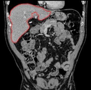
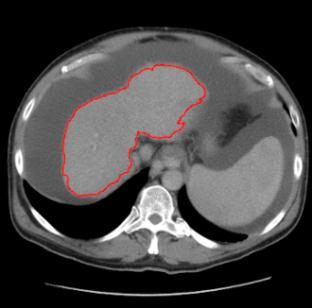
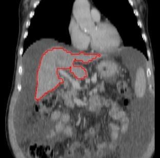
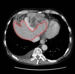
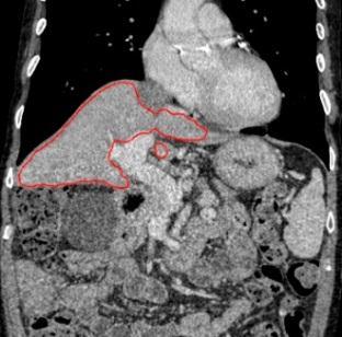
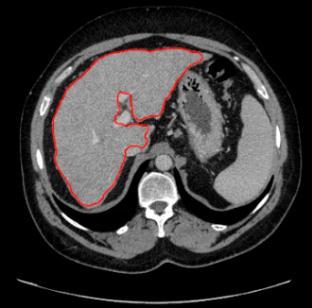
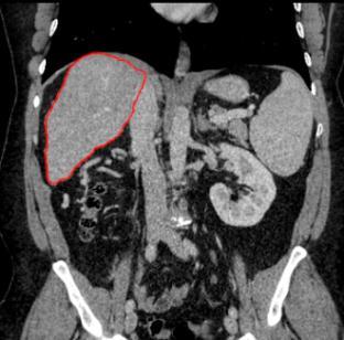
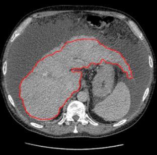
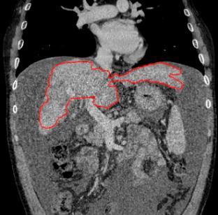
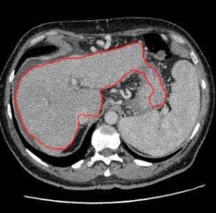
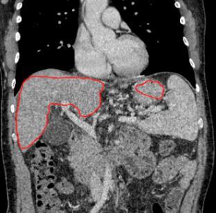
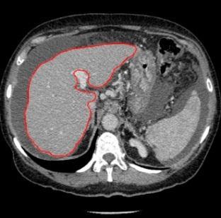
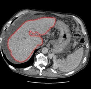
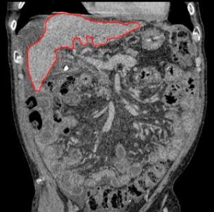
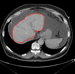
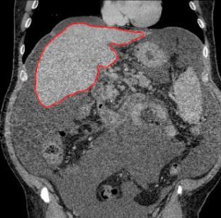
137 Appendix A Clinical study on liver volume measurement Table A.2 The result of the multi-phase liver segmentation method (red contour) for cases 1-10: each row presents 2 exams, where an axial (left) and a coronal (right) slice are displayed. 137

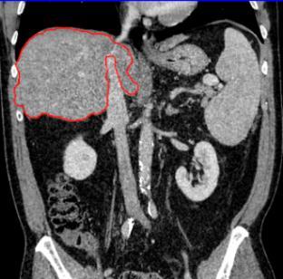
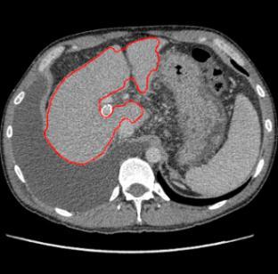
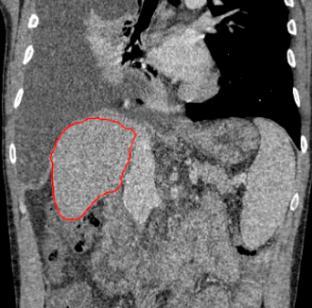
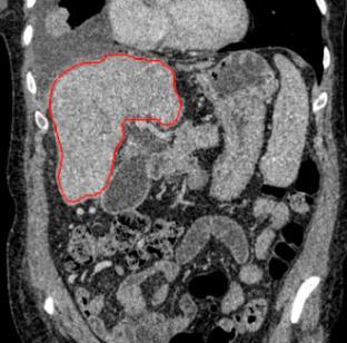
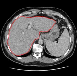
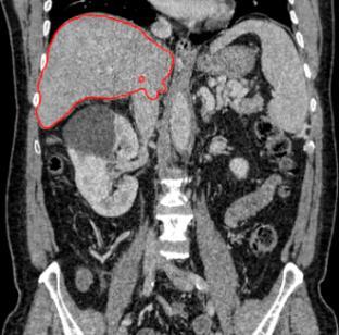
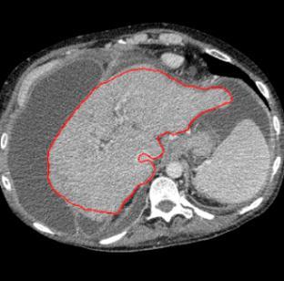
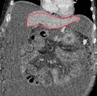
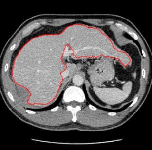
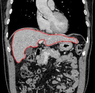
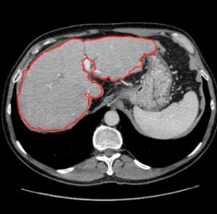
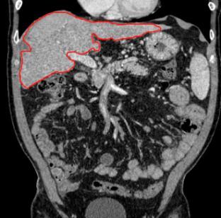
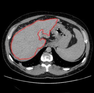
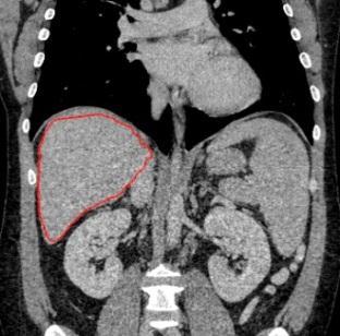
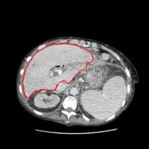
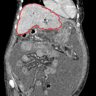
138 Appendix A Clinical study on liver volume measurement Table A.3 The result of the multi-phase liver segmentation method (red contour) for cases 11-20: each row presents 2 exams, where an axial (left) and a coronal (right) slice are displayed. 138

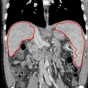
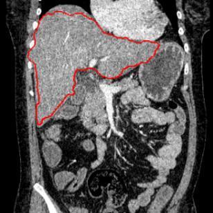
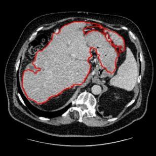
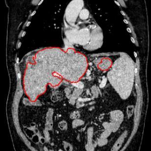
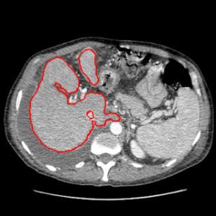
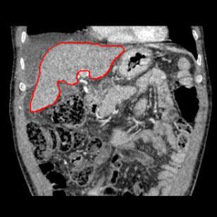
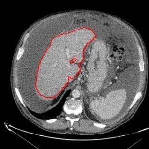
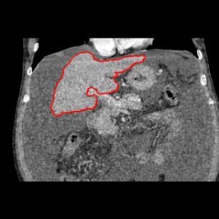
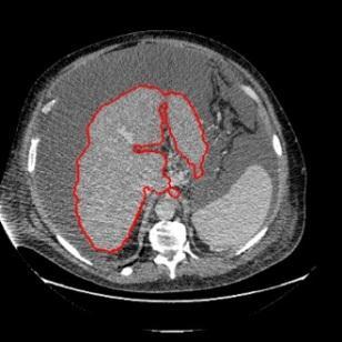
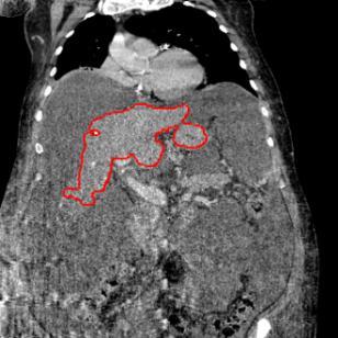
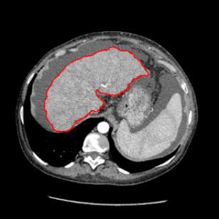
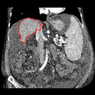
139 Appendix A Clinical study on liver volume measurement Table A.4 The result of the multi-phase liver segmentation method (red contour) for cases 21-30: each row presents 2 exams, where an axial (left) and a coronal (right) slice are displayed. 139

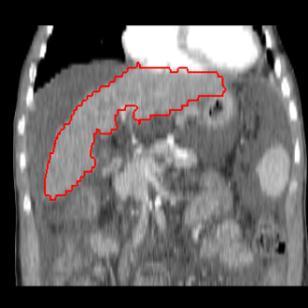
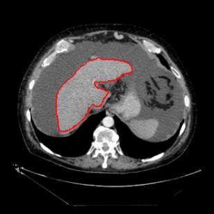
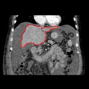
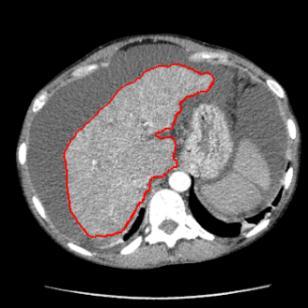
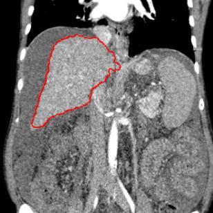
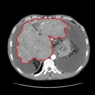
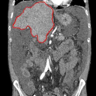
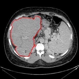
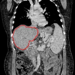
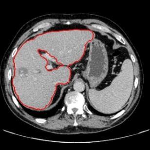
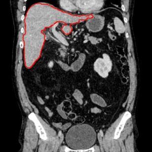
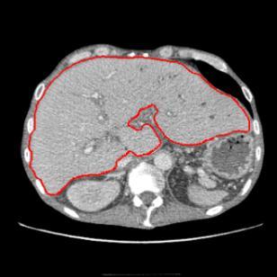
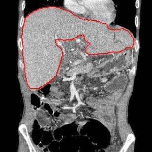
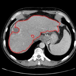
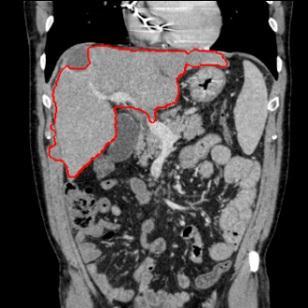
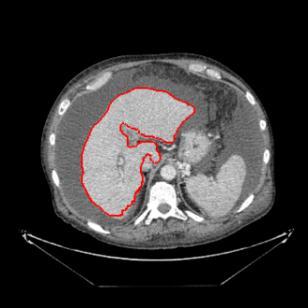
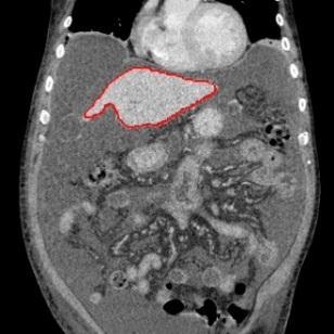
140 Appendix A Clinical study on liver volume measurement Table A.5 The result of the multi-phase liver segmentation method (red contour) for cases 31-40: each row presents 2 exams, where an axial (left) and a coronal (right) slice are displayed. 140