COMP3421. Global Lighting Part 2: Radiosity

Transcription

1 COMP3421 Global Lighting Part 2: Radiosity

2 Recap: Global Lighting The lighting equation we looked at earlier only handled direct lighting from sources: We added an ambient fudge term to account for all other light in the scene. Without this term, surfaces not facing a light source are black.

3 Global lighting In reality, the light falling on a surface comes from everywhere. Light from one surface is reflected onto another surface and then another, and another, and... Methods that take this kind of multi-bounce lighting into account are called global lighting methods.

4 Raytracing and Radiosity There are two main methods for global lighting: Raytracing models specular reflection and refraction. Radiosity models diffuse reflection. Both methods are computationally expensive and are rarely suitable for real-time rendering.

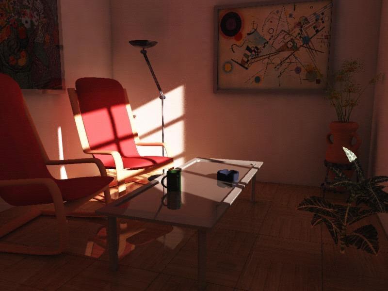
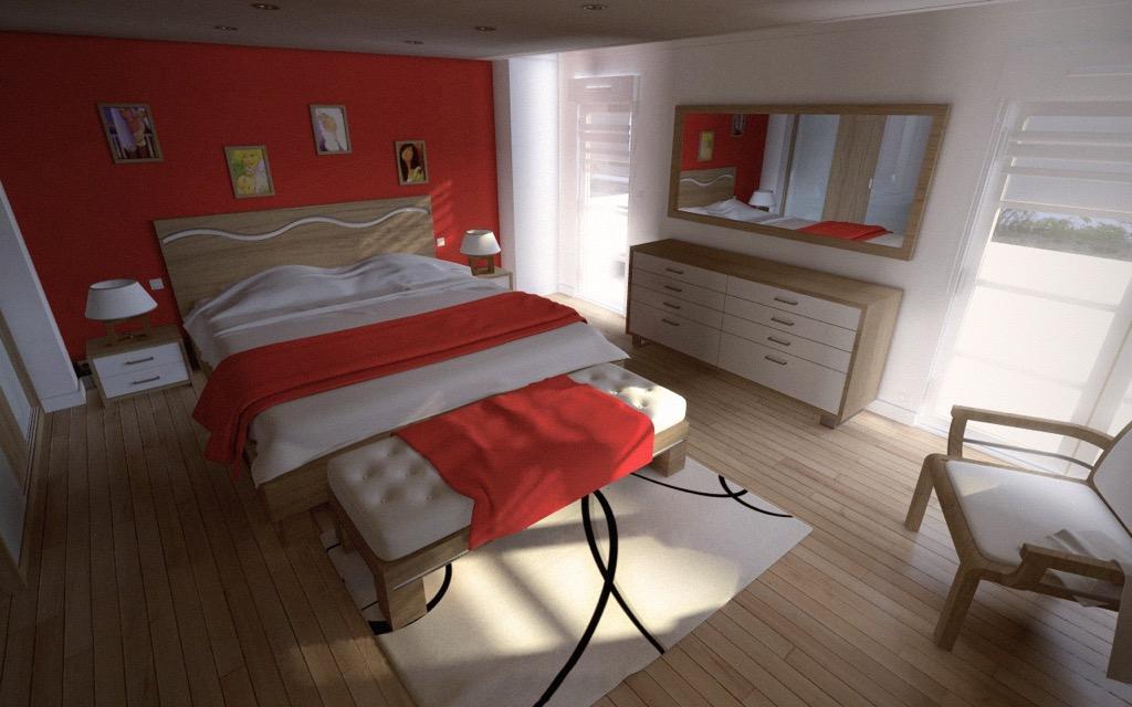
5 Radiosity Radiosity is a global illumination technique which performs indirect diffuse lighting. direct lighting + ambient global illumination

6 Radiosity Direct lighting techniques only take into account light coming directly from a source. Raytracing takes into account specular reflections of other objects. Radiosity takes into account diffuse reflections of everything else in the scene.

7 Ray tracing vs Radiosity incoming light incoming light n reflected light Specular reflection reflected light Diffuse reflection

8 Ray tracing vs Radiosity incoming light incoming light n reflected light Specular reflection view Diffuse reflection

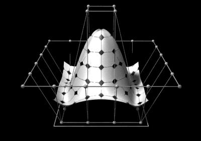
9 Finite elements We can solve the radiosity problem using a finite element method. We divide the scene up into small patches. We then calculate the energy transfer from each patch to every other patch.

10 Energy transfer The basic equation for energy transfer is: where ρ is the diffuse reflection coefficient.

11 Energy transfer The light input to a patch is a weighted sum of the light output by every other patch. Bi is the radiosity of patch i Ei is the energy emitted by patch i ρi is the reflectivity of patch i Fij is a form factor which encodes what fraction of light from patch j reaches patch i.

12 Form factors The form factors Fij depend on the shapes of patches i and j the distance between the patches the relative orientation of the patches Aj ni r θj nj θi Ai

13 Form factors Mathematically: Calculating form factors in this way is difficult and does not take into account occlusion. Aj ni r θj nj θi Ai

14 Nusselt Analog An easier equivalent approach: 1.render the scene onto a unit hemisphere from the patch's point of view. 2.project the hemisphere orthographically on a unit circle. 3.divide by the area of the circle

15 Nusselt Analog Aj Fij A/B

16 The hemicube method A simpler method is to render the scene onto a hemicube and weight the pixels to account for the distortion.

17 Solving The system of equations can be expressed as a matrix equation: In practice n is very large making exact solutions impossible.

18 Iterative approximation One simple solution is merely to update the radiosity values in multiple passes: for each iteration: for each patch i: Bnew[i] = E[i] for each patch j: Bnew[i] += rho[i] * F[i,j] * Bold[j]; swap Bold and Bnew

19 F B

20 Iterative approximation Using direct rendering for each iteration: for each patch i: Bnew[i] = E[i] S = RenderScene(i,Bold) B = Sum of pixels in S Bnew[i] += rho[i]*b swap Bold and Bnew

21 Iterative approximation first pass (direct lighting) second pass (one bounce) third pass (two bounces)

22 16 th Pass

23 Progressive refinement The iterative approach is inefficient as it spends a lot of time computing inputs from patches that make minimal or no contribution. A better approach is to prioritise patches by how much light they output, as these patches will have the greatest contribution to the scene.

24 Progressive refinement for each patch i: B[i] = db[i] = E[i] iterate: select patch i with max db[i]: calculate F[i][j] for all j for each patch j: drad = rho[j] * B[i] * F[i][j] * A[j] / A[i] B[j] += drad db[j] += drad db[i] = 0

25 In practice Radiosity is computationally expensive, so rarely suitable for real-time rendering. However, it can be used in conjunction with light mapping.

26 The payoff

27

28

29 Geometric light sources

30 Sources radiosity.htm gr_lectures.html HyperGraph/radiosity/overview_2.htm gpugems2_chapter39.html

31 Real-time Global Illumination v=pq39xb7odh8

32 COMP3421 B-Splines

33 Quick Recap: Curves We want a general purpose solution for drawing curved lines and surfaces. It should: Be easy and intuitive to draw curves Support a wide variety of shapes, including both standard circles, ellipses, etc and "freehand" curves. Be computationally cheap.

34 Bézier curves Have the general form: where m is the degree of the curve and P0...Pm are the control points.

35 Bernstein polynomials where: is the binomial function.

36 Bernstein polynomials For the most common case, m = 3:

37 Problems Local control - Moving one control point affects the entire curve. Incomplete - No circles, elipses, conic sections, etc.

38 Problem: Local control These curves suffer from non-local control. Moving one control point affects the entire curve. Each Bernstein polynomial is active (non-zero) over the entire interval [0,1]. The curve is a blend of these functions so every control point has an effect on the curve for all t from [0,1]

39 Splines A spline is a smooth piecewise-polynomial function (for some measurement of smoothness). The places where the polynomials join are called knots. A joined sequence of Bézier curves is an example of a spline.

40 Local control A spline provides local control. A control point only affects the curve within a limited neighbourhood.

41 Bézier splines We can draw longer curves as sequences of Bézier sections with common endpoints:

42 Parametric Continuity A curve is said to have C n continuity if the nth derivative is continuous for all t: C 0: the curve is connected. C 1: a point travelling along the curve doesn't have any instantaneous changes in velocity. C2: no instantaneous changes in acceleration

43 Geometric Continuity A curve is said to have G n continuity if the normalised derivative is continuous for all t. G 1 means tangents to the curve are continuous G 2 means the curve has continuous curvature.

44 Continuity Geometric continuity is important if we are drawing a curve. Parametric continuity is important if we are using a curve as a guide for motion.

45 Bézier splines If the control points are collinear, the the curve has G 1 continuity:

46 Bézier splines If the control points are collinear and equally spaced, the curve has C 1 continuity:

47 B-splines We can generalise Bézier splines into a larger class called basis splines or B-splines. A B-spline of degree m has equation: where L is the number of control points, with

48 B-splines The function is defined recursively: (Note: this formulation differs slightly from the one in the textbook)

49 Knot vector The sequence is called the knot vector. The knots are ordered so Knots mark the limits of the influence of each control point. Control point Pk affects the curve between knots tk and tk+m+1.

50 Number of Knots The number of knots in the knot vector is always equal to the number of control points plus the order of the curve. E.g., a cubic (m=3) with five control points has 9 items in the knot vector. For example: (0,0.125,0.25,0.375,0.5,0.625,0.75,0.875,1)

51 Uniform / Non-uniform Uniform B-splines have equally spaced knots. Non-uniform B-splines allow knots to be positioned arbitrarily and even repeat. A multiple knot is a knot value that is repeated several times. Multiple knots create discontinuities in the derivatives.

52 Continuity A polynomial of degree m has C m continuity. A knot of multiplicity k reduces the continuity by k. So, a uniform B-spline of degree m has C m-1 continuity.

53 Interpolation A uniform B-spline approximates all of its control points. A common modification is to have knots of multiplicity m+1 at the beginning and end in order to interpolate the endpoints. This is called clamping.

54 Moving Controls and Knots Moving Controls: Adjacent control points on top of one another causes the curve to pass closer to that point. With m adjacent control points the curve passes through that point. Moving Knots: Across a normal knot the continuity for and degree curve is C m-1. Each extra knot with the same value reduces continuity at that value by one.

55 Quadratic and Cubic The most commonly used B-splines are quadratic (m=2) and cubic (m=3). Uniform quadratic splines have C 1 (and G 1 ) continuity. Uniform cubic splines have C 2 (and G 2 ) continuity.

56 Bezier and B-Spline A Bézier curve of degree m is a clamped uniform B-spline of degree m with L=m+1 control points. A Bézier spline of degree m is a sequence of bezier curves connected at knots of multiplicity m. A quadratic piecewise Bézier knot vector with seven control points will look like this [ ].

57 Stop. Demo Time.

58 Incomplete Conic sections are what happens when a cone intersects a plane.

59 Rational Bézier Curves We can create a greater variety of curve shapes if we weight the control points: A higher weight draws the curve closer to that point. This is called a rational Bézier curve.

60 Rational Bézier Curves Rational Bézier curves can exactly represent all conic sections (circles, ellipses, parabolas, hyperbolas). This is not possible with normal Bézier curves. If all weights are the same, it is the same as a Bezier curve

61 Rational B-splines We can also weight control points in B-splines to get rational B-splines:

62 NURBS Non-uniform rational B-splines are known as NURBS. NURBS provide a power yet efficient and designer-friendly class of curves.

63 Closed curves A unclamped uniform B-spline of degree m is a closed loop if the first m control points match the last m control points.

64 Surfaces

65 Surfaces We can create 2D surfaces by parameterising over two variables: Where is any particular spline function we choose (Bezier, B-spline, NURBS) and denote an LxM array of control points.