LOCAL, SEMI-LOCAL AND GLOBAL MODELS FOR TEXTURE, OBJECT AND SCENE RECOGNITION

Transcription

1 LOCAL, SEMI-LOCAL AND GLOBAL MODELS FOR TEXTURE, OBJECT AND SCENE RECOGNITION Svetlana Lazebnik, Ph.D. Department of Computer Science University of Illinois at Urbana-Champaign, 2006 Jean Ponce, Advisor This dissertation addresses the problems of recognizing textures, objects, and scenes in photographs. We present approaches to these recognition tasks that combine salient local image features with spatial relations and effective discriminative learning techniques. First, we introduce a bag of features image model for recognizing textured surfaces under a wide range of transformations, including viewpoint changes and non-rigid deformations. We present results of a large-scale comparative evaluation indicating that bags of features can be effective not only for texture, but also for object categization, even in the presence of substantial clutter and intra-class variation. We also show how to augment the purely local image representation with statistical co-occurrence relations between pairs of nearby features, and develop a learning and classification framework for the task of classifying individual features in a multi-texture image. Next, we present a more structured alternative to bags of features for object recognition, namely, an image representation based on semi-local parts, or groups of features characterized by stable appearance and geometric layout. Semi-local parts are automatically learned from small sets of unsegmented, cluttered images. Finally, we present a global method for recognizing scene categories that works by partitioning the image into increasingly fine sub-regions and computing histograms of local features found inside each sub-region. The resulting spatial pyramid representation demonstrates significantly improved performance on challenging scene categorization tasks.

2 LOCAL, SEMI-LOCAL AND GLOBAL MODELS FOR TEXTURE, OBJECT AND SCENE RECOGNITION BY SVETLANA LAZEBNIK B.S., DePaul University, 2000 M.S., University of Illinois at Urbana-Champaign, 2002 DISSERTATION Submitted in partial fulfillment of the requirements for the degree of Doctor of Philosophy in Computer Science in the Graduate College of the University of Illinois at Urbana-Champaign, 2006 Urbana, Illinois

3 c Copyright by Svetlana Lazebnik, 2006

4 ABSTRACT This dissertation addresses the problems of recognizing textures, objects, and scenes in photographs. We present approaches to these recognition tasks that combine salient local image features with spatial relations and effective discriminative learning techniques. First, we introduce a bag of features image model for recognizing textured surfaces under a wide range of transformations, including viewpoint changes and non-rigid deformations. We present results of a large-scale comparative evaluation indicating that bags of features can be effective not only for texture, but also for object categization, even in the presence of substantial clutter and intra-class variation. We also show how to augment the purely local image representation with statistical co-occurrence relations between pairs of nearby features, and develop a learning and classification framework for the task of classifying individual features in a multi-texture image. Next, we present a more structured alternative to bags of features for object recognition, namely, an image representation based on semi-local parts, or groups of features characterized by stable appearance and geometric layout. Semi-local parts are automatically learned from small sets of unsegmented, cluttered images. Finally, we present a global method for recognizing scene categories that works by partitioning the image into increasingly fine sub-regions and computing histograms of local features found inside each sub-region. The resulting spatial pyramid representation demonstrates significantly improved performance on challenging scene categorization tasks. iii

5 To Max iv

6 ACKNOWLEDGMENTS The research presented in this dissertation was partially supported by the National Science Foundation under grants IIS , ITR and IIS , Toyota, the UIUC Campus Research Board, the Beckman Institute for Advanced Science and Technology, the UIUC-CNRS collaboration agreement, and the European project LAVA. I would also like to acknowledge the UIUC Computer Science Department and the College of Engineering for supporting me with the SURGE fellowship and various awards. I am grateful to all the members of my Ph.D. thesis committee, and especially to Jean Ponce and Cordelia Schmid, for guiding and encouraging my research. I would also like to thank Marcin Marszalek and Jianguo Zhang for implementing extensions to my texture recognition methods and providing the experimental results for Section 3.2. Everlasting gratitude is due to my wonderful husband Maxim Raginsky and to the rest of my family, including my sister Maria (who will herself be defending her Ph.D. a year or two from now), my parents, and grandmother. v

7 TABLE OF CONTENTS CHAPTER PAGE 1 Introduction RecognitionTasks TextureRecognition ObjectRecognition SceneRecognition Themes,ContributionsandOutline Previous Work FeatureDetectorsandDescriptors TextureRecognition ObjectRecognition SceneandContextRecognition A Bag-of-Features Model for Texture and Object Recognition TextureRecognitionUsingLocalAffineRegions ComponentsoftheApproach AffineRegionDetection Rotation-InvariantDescriptors SignaturesandtheEarthMover sdistance ExperimentalEvaluation EvaluationStrategy UIUCTextureDatabase BrodatzDatabase AnExtendedEvaluation: FromTexturetoObjectRecognition Kernel-basedclassification TextureRecognition ComparingInvarianceLevelsandDescriptorTypes Comparative Evaluation: UIUC Database, Brodatz, CUReT Object Recognition: Caltech6, Caltech101, Graz Discussion vi

8 4 Neighborhood Co-occurrence Relations for Texture Recognition A Maximum Entropy Framework for Combining Local Features and Their Relations TheMaximumEntropyClassifier TextonVocabularyandFeatureFunctions ExperimentalResults: UIUCDatabaseandBrodatz ATwo-StageApproachforRecognizingLocalTextureRegions ModelingTextures DensityEstimation NeighborhoodStatistics Relaxation ClassificationandRetrieval ExperimentalResults TheIndoorScene Animals Discussion Semi-Local Parts for Object Recognition Motivation Semi-LocalParts MatchingofPairsofImages Validation Recognition RecognitionExperiments Affine-InvariantParts Scale-InvariantParts Discussion Spatial Pyramid Matching for Scene Recognition Motivation SpatialPyramidMatching PyramidMatchKernels SpatialMatchingScheme FeatureExtraction Experiments SceneCategoryRecognition Caltech TheGrazDataset Discussion Conclusion Summary Extensions vii

9 APPENDIX A Harris and Laplacian Region Detectors A.1 SpatialandScaleSelection A.2 AffineAdaptation REFERENCES AUTHOR S BIOGRAPHY viii

10 CHAPTER 1 Introduction The recognition of materials, objects, and scene categories from photographs are among the most central problems in the field of computer vision. However, despite decades of intensive research, even the most sophisticated recognition systems today (see [139] for a summary of the state of the art) remain incapable of handling more than just a few simple classes, or of functioning under unconstrained real-world conditions. What makes recognition so difficult is the seemingly limitless variability of natural imagery that arises from viewpoint and lighting changes, movement and deformation of non-rigid or articulated objects, intraclass appearance variations, and the presence of occlusion and background clutter (see Figure 1.1 for examples of different kinds of visual classes with some representative variations). This dissertation proposes novel models of image content that are robust to many of these sources of variability and can achieve high recognition performance on challenging datasets. As basic building blocks for our models, we use local image features, or appearance-based descriptors computed over regions of support whose size is typically much smaller than that of the entire image. As shown in Figure 1.2, a patch-based description or representation of an image can be obtained by processing the image with one of the specialized scale- or affineinvariant salient region detectors that have been introduced over the last decade [61, 62, 83, 90, 101, 104, 153]. Alternatively, for applications that do not require geometric invariance, we can simply sample rectangular patches randomly [100] or on a regular grid [30]. In recent literature, local features have been used for image indexing and retrieval [103, 137, 138], 1

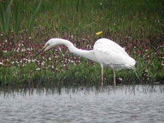
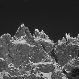
11 Texture and material recognition: Textured surfaces may be photographed in a wide range of scales and orientations, and significant perspective distortions may be present in images. Some materials, like marble, are highly nonhomogeneous, and others, like cloth, are non-rigid. Object recognition: Objects may be difficult to detect because of clutter and occlusion. Animals are non-rigid and appear in different poses. Some classes, like giraffes, can be characterized well by their texture, but others, like egrets, are textureless and require a more structured representation. Scene recognition: Natural scene categories have significant intra-class variation. Some indoor categories, such as kitchen and living room, may be difficult to distinguish from one another. Figure 1.1 Examples of images for each of the recognition tasks considered in this dissertation. 2

12 Figure 1.2 Two alternative patch-based representations of two natural images. Left: original images, center: patches found by the Harris detector, right: patches found by the Laplacian detector. wide-baseline matching [3, 134, 135, 153], description and matching of video clips [129, 144], recognizing different views of the same object [34, 130] and different instances of the same object class [1, 23, 33, 163]. Indeed, using local features as image primitives has several important advantages: Robustness: Because local features are relatively small and compact, they can be preserved even when large portions of an image are affected by clutter or occlusion. Repeatability: Many existing local feature detectors can reliably identify corresponding features in different images despite geometric transformations, changes in lighting, or minor appearance variations. These may be features corresponding to the same surface patch in two views of the same object, or features corresponding to analogous structures, such as eyes, on different instances of the same class. 3

13 Expressiveness: Unlike the geometric features historically used in computer vision (points or line segments), today s local features contain information not only about their shape (circular, elliptical, or rectangular), but also about their appearance. Rich high-dimensional descriptors of appearance provide strong consistency constraints for matching tasks. Local geometric invariance: Depending on the requirements of a particular application, one may choose to use scale-, rotation- or affine-invariant local features. In particular, affine invariance offers robustness to a wide range of geometric transformations that can be locally approximated by a linear model, including perspective distortions and non-rigid deformations. Compactness or sparsity: The number of features returned by most detectors is typically orders of magnitude smaller than the total number of pixels in the original image. The resulting patch-based description is extremely compact, thus reducing processing time and storage requirements. In this dissertation, we present several novel approaches for modeling visual classes. These approaches can be classified into three types, based on the kinds of geometric relations between local features that they encode (Figure 1.3): local models disregard all spatial information; semi-local models capture relations between groups of nearby regions; and global models encode the spatial layout of all features in the image. In our work, local models (Chapter 3) are aimed primarily at texture recognition, though in Section 3.2, we show them to be surprisingly effective for object categorization as well. Semi-local models (Chapter 5) are used to create a part-based object representation. Finally, global models (Chapter 6) are used to describe scenes, though they can also work well for recognizing object classes in the absence of geometric deformations. The next section discusses the tasks of texture, object and scene recognition in more detail, together with their associated models. 4

14 Local model Semi-local model Global model Figure 1.3 The three kinds of models used in this thesis. Top left: a local model is a distribution or histogram of appearance descriptors of salient regions extracted from the image. This model is most appropriate for texture recognition. Top right: a semi-local model is a geometrically stable group of neighboring local features lying on the object of interest. We use semi-local parts to represent object structure. Bottom: a global model is a set of histograms computed over a multi-level pyramid decomposition of the image. This model is most effective for scene recognition. 5

15 1.1 Recognition Tasks Texture Recognition We want to recognize images of textured surfaces subject to viewpoint changes and nonrigid deformations. For this task, we use a local model in which spatial constraints are absent, i.e., each patch is considered separately, without any information about its neighborhood or its position in the image. In the framework presented in Chapter 3, each image is represented by the distribution of appearance descriptors of the features contained in it. The distribution is learned by quantizing the descriptors in the image and forming a signature, orasetofall cluster centers together with weights indicating the relative sizes of the clusters. Signatures of different images are compared using Earth Mover s Distance (EMD) [131, 132], which solves a partial matching problem between sets of possibly unequal cardinality, and is robust to noise, clutter, and outliers. We also investigate an alternative bag-of-features approach, in which local features are quantized into textons or visual words drawn from some universal vocabulary, and their distributions in images are represented as histograms of texton labels. This approach is analogous to the bag-of-words paradigm for text document analysis [9, 52, 102, 114, 133]. A major shortcoming of bag-of-features methods is their disregard of spatial relations. For many natural textures, the spatial layout of local features captures perceptually important information about the class. Augmenting our texture representation with geometric information can be expected to increase its ability to discriminate between textures that have similar local elements but different geometric patterns. In the first part of Chapter 4, we present a texton-and-relations model that takes inspiration from bigram models used to describe text documents. Specifically, our model represents not only the frequencies of individual textons, but also the frequencies of co-occurrences of pairs of texton labels at nearby locations in the image. In the second part of Chapter 4, we consider the task of labeling individual features in multi-texture images. This task is more challenging than classification 6

16 of single-texture images, because the local appearance of the feature itself is often insufficiently discriminative (for example, if we observe a uniformly blue image patch, we do not know whether it is water or sky). To reduce this ambiguity, we introduce a two-level model that first computes the probabilities of class membership of individual regions using a purely local model, and then refines these probabilities using a relaxation framework that relies on spatial relations to obtain contextual information Object Recognition Our second target problem is recognizing object categories despite 3D viewpoint changes, intra-class appearance variations, non-rigid motions, as well as clutter and occlusion in the test images. At the most basic level, object recognition may be considered as a whole-image classification problem, i.e., identifying which object class is present in an image, without attempting to segment or localize that object. For this (admittedly simplified) task, it is possible to represent the visual texture of images containing objects using the orderless bagof-features model described in Section Such models have been used in several recent approaches to visual categorization [20, 164], unsupervised discovery of visual topics [30, 122, 143], and video retrieval [144]. In these publications and in the evaluation presented in the second half of Chapter 3, orderless models have achieved surprisingly high levels of accuracy on several challenging datasets. Despite its practical advantages, a bag of features is an extremely impoverished representation for object classes, since it ignores all geometric information about the object class, fails to distinguish between foreground and background features, and cannot segment an object from its surroundings. In chapter 5, we propose a more structured object representation basedoncompositesemi-local parts, defined as geometrically stable configurations of multiple local features that are robust against approximately rigid deformations and intra-class variations. An object model consists of a collection of multiple semi-local parts, and these 7

17 parts, in turn, can be connected to each other by looser geometric relations. Semi-local parts are detected using an alignment-like geometric search, which can in principle work with any rigid 2D transformation model, from translation to projective (in the experiments presented in Chapter 5, we demonstrate scale- and affine-invariant parts). Note, however, that in searching for semi-local parts, we do not assume that the entire object of interest is globally planar and/or rigid, only that it possesses some sub-components that can be approximately characterized in this way. Thus, our approach extends the level of geometric invariance of existing part-based object models [1, 28, 33, 163] which are mostly limited to recognizing fronto-parallel views of upright objects. Our learning framework does not require objects in training images to be hand-segmented or hand-aligned, it can work with minimal amounts of training data, and is robust to substantial noise, background variation, and occlusion Scene Recognition Our third problem is recognizing semantic scene categories such as beach, mountain, school, office, etc. Just as texture and object recognition, this task can be approached using purely local models [30, 91]. However, in this dissertation we show that improved performance can be achieved by a global model that takes into account the absolute positions of the features. Intuitively, a global model has improved discriminative power because it captures spatial regularities that are important to our perception of natural scenes (for example, sky is usually above ground or water, building walls are usually vertical, the horizon is usually a horizontal line, etc.). In Chapter 6, we propose a spatial pyramid model that is based on forming a multi-level quadtree decomposition of an image and aggregating statistics of local features over each cell of the decomposition at each level (Figure 1.3, bottom). This approach is inspired by the pyramid matching framework of Grauman and Darrell [45], who form a multi-scale decomposition of the high-dimensional space of appearance descriptors, instead of the two-dimensional image space. Note that the number of levels in the image 8

18 decomposition is an implementation parameter of our approach; the higher it is, the more precisely individual features are localized. When the number of levels is zero, the spatial pyramid representation reduces to a standard bag of features. Our experiments demonstrate that the spatial pyramid achieves a significant improvement in performance over bags of features not only for scene classification tasks, but also for object classification tasks that do not require geometric invariance. 1.2 Themes, Contributions and Outline The recognition approaches presented in this dissertation are based on combining salient local features with various kinds of geometric relations and effective discriminative learning techniques. Let us briefly discuss the major issues or themes associated with each of these components. When dealing with local features, we are usually most concerned with the issue of invariance. In computer vision literature, there exist feature extraction schemes that are invariant to scaling, scaling with rotation, and to affine transformations (see Section 2.1 for a literature review). As discussed in Chapter 3, by using these features, we can compensate for various geometric transformations in the images, from global scale changes, rotations and affine deformations, to perspective changes and even non-rigid distortions. Given datasets that contain a wide range of these transformations, approaches that do not have intrinsically invariant features are at a disadvantage, since they require training exemplars to sample all the possible changes that may appear in the test set. Thus, with geometrically invariant features, we can learn from much smaller training sets. However, there is a tradeoff: the higher the level of invariance, the greater the amount of discriminative information that is lost during the feature normalization process. In the course of the experimental evaluation reported in Section 3.2, we have found that the best results are usually achieved with the lowest level of invariance absolutely required for a given application. Finally, in some ap- 9

19 plications such as scene recognition (Chapter 6), the sources of intra-class variability are so complex that they are best dealt with by statistical methods instead of geometric ones. In these cases, invariant features are not likely to bring much of a benefit at all, and an exemplar-based approach is more appropriate. Another theme that runs through this dissertation is that of matching or correspondence. The bag-of-features method of Chapter 3 is based on comparing distributions of features in two images. To perform this comparison, we represent the distributions as two discrete sets of points in high-dimensional appearance space and use the Earth Mover s Distance (EMD) to find the lowest-cost matching between these two sets. Note that in this case, the matching does not take into account any spatial information. By contrast, our global model of Chapter 6 is based on the idea of matching two sets of features in image space, not in appearance space. Since our target application of scene recognition requires only a rough notion of spatial consistency, we obtain an efficient approximation to the matching cost using a pyramid match kernel that can also be used to approximate EMD [45]. Finally, our part-based object recognition approach of Chapter 5 uses a much more precise operation of matching two sets of features that have consistent appearance and geometric layout. We implement this operation as a constrained alignment search. While it is more computationally expensive than pyramid matching, it has the advantage of providing us with explicit correspondences, and also allowing us to match groups of features that have been subjected to (approximately rigid) affine transformations. An important unifying theme associated with the learning component of our methods is our emphasis on weakly supervised learning, i.e., the ability to construct texture, object and scene models from unsegmented and cluttered training images. Today, fully supervised learning is still the standard for many recognition approaches it is routine, for example, to hand-segment training images and hand-label individual features as belonging to various object classes. However, the effort and expense associated with these tasks will make detailed 10

20 annotation impractical for the large-scale datasets that vision algorithms will have to handle in the future. Therefore, reducing the amount of manual supervision required by vision systems is crucial for enabling them to function in real-world applications. The main contributions of this dissertation can be summarized as follows: Our approach to texture recognition (Chapter 3) is the first one to rely on local features produced by scale- and affine-invariant interest region detectors. The resulting texture representation is intrinsically invariant to a wide range of geometric transformations, and therefore can be learned from relatively few images, unlike other existing approaches, which require exemplars of every possible transformation to be included in the training set. In Section 3.2, we extend our bag-of-features method with a Support Vector Machine (SVM) classifier, and the resulting system outperforms other state-of-the-art approaches on several challenging object databases. This part of our work is performed in collaboration with Jianguo Zhang and Marcin Marszalek at INRIA Rhône-Alpes. To our knowledge, our approach for labeling individual texture regions (Section 4.2) is the only one to date that can learn texture models in a weakly supervised manner, i.e., from multi-texture images that are not segmented, only labeled by the textures that they contain. Our object representation in terms of semi-local parts (Chapter 5) has a number of advantages over constellation models [163, 33] and methods based on low-distortion correspondence [5]: it does not assume that the object is globally planar and/or rigid, it can achieve a higher degree of geometric invariance (up to affine, which can approximate viewpoint changes), and can tolerate a much greater degree of clutter during learning. The spatial pyramid method introduced in Chapter 6) is a simple, yet effective extension of the basic bag-of-features model, capable of achieving significantly higher 11

21 performance on scene classification, and on object classification in the absence of clutter and geometric variation. In particular, our method exceeds the state of the art on the Caltech101 dataset [29]. The rest of this dissertation is organized as follows. Chapter 2 reviews existing computer vision literature on local image features, as well as methods for texture, object, and scene recognition. Chapter 3 presents our bag-of-features model for texture and object classification. Chapter 4 describes two extensions to this model that incorporate pairwise relations between nearby features. Chapter 5 presents our representation of object classes in terms of semi-local parts, and Chapter 6 presents our global spatial pyramid model for scene classification. Finally, Chapter 7 closes the dissertation with a summary of our contributions and discussion of possible extensions and future research directions. The work described in this dissertation has been previously published in [71, 72, 73, 74, 75, 76, 168]. 12

22 CHAPTER 2 Previous Work This chapter reviews existing work on feature detectors and descriptors, as well as methods for texture, object, and scene recognition. 2.1 Feature Detectors and Descriptors Early work on the extraction of local features in natural images includes the interest operators of Moravec [108] and Harris [50], as well as various image decompositions into perceptually salient blob-like primitives [19, 95, 160]. Blostein and Ahuja [10] were the first to introduce a multiscale blob detector based on maxima of the Laplacian. Lindeberg [82] has extended this detector in the framework of automatic scale selection, where a blob is defined by a scale-space location where a normalized Laplacian measure attains a local maximum. Informally, the spatial coordinates of the maximum become the coordinates of the center of the blob, and the scale at which the maximum is achieved becomes its characteristic scale. Gårding and Lindeberg [40] have also shown how to design an affine blob detector using an affine adaptation process based on the second moment matrix. This process forms an important part of two affine-invariant 1 region detection schemes [3, 104] that rely on a multiscale version of the Harris operator to localize interest points in space. 1 It is more technically correct to refer to these regions as affine-covariant, which means that the regions detected in an affinely transformed version of an image can be obtained by subjecting the regions found in the original image to the same transformation. However, the term affine-invariant is common in the literature [104, 105], and so we use it throughout this dissertation for consistency. 13

23 Shape Context SIFT Figure 2.1 The decomposition of the region of support used by the shape context (left) and the SIFT descriptor (right). In the work presented in Chapters 3-5 of this dissertation, we use the Laplacian detector of Gårding and Lindeberg [40] and the Harris detector of Mikolajczyk and Schmid [104, 105]. A brief description of these detectors, including details of the scale selection and affine adaptation procedures mentioned above, is given in the Appendix. Alternative region extraction schemes include the entropy detector of Kadir and Brady [62], the differenceof-gaussians (or DoG) detector of Lowe [90] (see also Crowley and Parker [19] for related work), the maximally stable extremal regions of Matas et al. [101], and the corner- and intensity-based operators of Tuytelaars and Van Gool [153]. Of the above, [62, 90] are scaleinvariant, while [101, 153] are fully affine-invariant. This proliferation of region detectors, motivated primarily by applications to wide-baseline stereo matching and image retrieval, attests to the increased importance accorded to the spatial and shape selection principles in the computer vision community. A comparative evaluation of several state-of-the-art region detectors is presented in [107]. Detection of local image regions is only the first part of the feature extraction process; the second part is the computation of descriptors to characterize the appearance of these regions. A good descriptor should be distinctive, so as to provide strong consistency constraints for image matching, yet robust to illumination changes and other nuisance appearance 14

24 variations. A classic method of image description is in terms of differential invariants derived from the local jet, or the vector of image derivatives computed up to a specified order [65]. Another classic method is to describe the appearance of an image region by the outputs of a set of linear filters, such as Gabor filters [39, 98], wavelets [158], or steerable filters [37]. In current literature, there exists a wide variety of filter banks custom-engineered for specific applications (see [125] for a survey). Despite the historical popularity of filter banks, they do not always provide the best method of image description. For example, it has been shown that raw pixel values can be more effective than filter outputs for texture classification [157]. In recent literature, very promising results have been achieved by so-called distribution-based descriptors [106], such as the shape context [4] and the Scale-Invariant Feature Transform (SIFT) [89, 90], that work by subdividing the region of support and counting appearance attributes (edge points or oriented edge points) inside each subregion. The shape context uses a log-polar decomposition of a circular image region, and computes counts of edge points in each spatial bin. The example in Figure 2.1, left uses 12 angular bins and 4 radial bins, for a 48-dimensional descriptor. The SIFT descriptor (Figure 2.1, right) divides a square patch into a 4 4 grid and computes a histogram of gradient orientations in each subregion. Eight gradient orientations are used, resulting in a 128-dimensional feature vector. Histogramming provides stability against deformations of the image pattern, while subdividing the support region offsets the potential loss of spatial information. In this way, a compromise is achieved between the conflicting requirements of greater geometric invariance on the one hand and greater discriminative power on the other. Intuitively, descriptors based on this compromise should be simultaneously richer and more robust than filter banks and differential invariants, which are functions of the entire region of support. Indeed, in a recent comparative evaluation [106], SIFT descriptors and shape contexts decisively outperform these more traditional methods. In Section , we introduce two new distribution-based 15

25 descriptors, spin image and RIFT, that are tailored to achieve greater geometric invariance and computational efficiency as opposed to greater distinctiveness. 2.2 Texture Recognition The automated analysis of image textures has been the topic of extensive research in the past forty years, dating back at least to Julesz in 1962 [59]. Traditional techniques for modeling texture include co-occurrence statistics [49, 59], filter banks [97, 125], and random fields [99, 167]. One of the most important challenges in the field of texture analysis and recognition is achieving invariance to a wide range of geometric and photometric transformations. Early research in this domain has concentrated on global 2D image transformations, such as rotation and scaling [18, 99]. However, such models do not accurately capture the effects of 3D transformations (even in-plane rotations) of textured surfaces. More recently, there has been a great deal of interest in recognizing images of textured surfaces subjected to lighting and viewpoint changes [21, 22, 80, 87, 156, 157, 165]. A few methods [80, 87, 165] are based on explicit reasoning about the 3D structure of the surface, which may involve registering samples of a material so that the same pixel across different images corresponds to the same physical point on the surface [80] or applying photometric stereo to reconstruct the depth map of the 3D texture [87, 165]. While such approaches capture the appearance variations of 3D surfaces in a principled manner, they require specially calibrated datasets collected under controlled laboratory conditions. For example, the 3D texton representation of Leung and Malik [80] naturally lends itself to the task of classifying a stack of registered images of a test material with known imaging parameters, but its applicability is limited in most practical situations. In our own work, we are interested in classifying unregistered texture images. This problem has been addressed by Cula and Dana [21] and Varma and Zisserman [156, 157], who have developed several dense 2D texton-based representations capable of very high accuracy 16

26 on the challenging Columbia-Utrecht reflectance and texture (CUReT) database [22]. The descriptors used in these representations are filter bank outputs [21, 156] and raw pixel values [157]. Even though these methods have proven effective in the complex task of classifying images of materials despite significant appearance changes, the representations themselves are not invariant to the changes in question. In particular, the support regions for computing descriptors are the same in all images; no adaptation is performed to compensate for changes in surface orientation with respect to the camera. Because they lack representation-level invariance, the above methods require the use of multiple models or prototypes to represent a single texture. As long as the training set adequately samples all viewpoints and lighting directions that can be encountered at test time, the texture can be successfully recognized. On the other hand, when the test set contains images not represented in the training set (e.g., images at significantly different scales), performance drops dramatically [156]. In Chapter 3, we show how to reduce this dependence on representative training sets by developing a texture representation with builtin geometric invariance. 2.3 Object Recognition The earliest recognition systems [13, 88, 112, 127] were model-based, i.e., designed to perform localization and pose estimation from a single view of an object given a representation of its 3D shape (possibly as a combination of parts or geometric primitives such as generalized cylinders). This work has emphasized the relatively abstract issues of viewpointindependent representation of generic 3D shapes and formal rule-based geometric reasoning. While model-based vision systems represent important conceptual milestones in the field of recognition, their practical usefulness is severely limited by their reliance on relatively weak and uninformative image features such as line and curve segments and their lack of flexibility for modeling non-parametric deformations or complex intra-class variations (though 17

27 some model-based approaches [170] have made a systematic attempt to represent deformable objects such as animals from their 2D silhouettes). In this dissertation, we follow instead an alternative appearance-based recognition paradigm, which emphasizes not precise 3D geometric description, but statistical modeling of 2D object apperance using highly expressive and discriminative image features. Initial work on appearance-based object recognition has mainly utilized global descriptions: The raw images themselves can be subjected to eigenspace analysis [110, 152] or used as feature vectors for support vector machine classification [120]. Another class of early methods [113, 136] is based on characterizing the entire image using color or texture histograms. The main drawback of such methods is their lack of robustness to clutter and occlusion. For this reason, recognition methods that work by characterizing the entire image have been gradually supplanted over the last decade by part-based methods that seek to identify statistically or structurally significant atoms of object appearance. In the older model-based literature, a part was usually understood to be a 3D geometric primitive in some formal scheme for representing general shapes. By contrast, appearance-based approaches have a much more flexible image-based notion of a part. Schneiderman and Kanade [140] define parts as groups of highly correlated input variables (in their case, wavelet coefficients). Most other approaches obtain parts by sampling image fragments [93, 142, 154], or by detecting corner-like interest points [1, 162, 163] or scale-invariant salient regions [29, 33]. In the current literature, a popular object recognition paradigm is that of probabilistic constellation or parts-and-shape models that represent not only the statistics of individual parts, but also their spatial layout [14, 29, 33, 163]. The idea of such models goes back at least thirty years to the pictorial structures of Fischler and Elschlager [35]. Unfortunately, the level of geometric invariance of existing constellation models is limited to scale and translation, since a principled probabilistic treatment of rotation or affine invariance is prohibitively complex [78]. Learning and inference problems for these models become even 18

28 more intractable in a weakly supervised setting where the location of the object in a training image has not been marked by hand. This setting requires the use of the Expectation Maximization (EM) algorithm [8] to perform the assignment of object parts to image regions in the presence of occlusion and clutter. However, the combinatorics of EM-based learning severely limits both the expressiveness of the corresponding object models and the amount of clutter and/or occlusion that can be tolerated during learning. In response to the above difficulties with parts-and-shape models, several vision researchers have proposed orderless bag-of-features models [20, 164, 143], which are obtained by extracting scale- or affine-invariant local features from images, quantizing them into visual words, and learning the distributions of these words for each object class. This is essentially the same strategy that we use in designing the local texture model presented in Chapter 3. However, while an orderless representation is appropriate for texture images, which lack clutter and have uniform statistical properties, it is somewhat problematic as a method for representing object classes, since it ignores spatial relations and makes no distinction between features generated by the object and those generated by the background. In fact, bag-offeatures methods are prone to much the same pitfalls as earlier global and histogram-based recognition approaches. One way to increase the robustness of bag-of-features methods to clutter and occlusion is to use statistical techniques such as feature selection [24] or boosting [118] to retain only the most discriminative features for recognition. Another solution is to design novel kernels that can yield high discriminative power despite the noise and irrelevant information that may be present in local feature sets [45, 92, 161]. In Chapter 3, we follow this idea by introducing a kernel based on EMD, which is designed for partial matching, and therefore performs well in clutter and occlusion. With the addition of this kernel, our local texture representation becomes capable of achieving and even exceeding state-of-the-art classification results on multiple object databases. 19

29 Even though we can obtain good object recognition results using a completely orderless method, our ultimate goal in this disseration is to overcome the limitations of Bayesian partsand-shape models without sacrificing spatial relations. We can achieve this by adopting a non-probabilistic approach to learning and detecting object parts that is based on direct search for visual correspondence. In recent literature, the low-distortion correspondence method of Berg et al. [5] is an example of this philosophy. In Chapter 5 we present an object representation in which composite parts are found using alignment techniques [54]. Our semi-local part approach is capable of a higher degree of geometric invariance than existing constellation models, and, in combination with a discriminative maximum entropy framework (Section 4.1), enables the learning of relatively complex object models consisting of many features in heavily cluttered images. 2.4 Scene and Context Recognition In the 1990s, several researchers have considered semantic scene categorization tasks such as distinguishing city views from landscapes [44, 155] and indoor from outdoor images [147]. Subsequent computational approaches to scene description and recognition have often drawn their inspiration from the literature on human perception. For example, it is known that people can recognize scenes by considering them in a holistic manner, without having to recognize individual objects [7]. Recently, it has been shown that human subjects can perform high-level categorization tasks extremely rapidly [148] and in the near absense of attention [31]. Renninger and Malik [126] propose an orderless bag-of-textons model to replicate human performance on rapid scene categorization tasks. Another perceptually inspired approach, due to Oliva and Torralba [117], computes a low-dimensional representation of a scene based on several global properties such as openness and ruggedness. A few recent scene recognition approaches [91, 159] try to find effective intermediate representations in terms of basic natural texture categories, such as water, sky, sand, grass, foliage, etc. A ma- 20

30 jor drawback of these methods is that these categories have to be learned in a fully supervised fashion, which requires human participants either to hand-segment the training images and label their constituent categories or to provide numerous sample patches of each category. Fei-Fei and Perona [30] present an alternative unsupervised approach that represents scenes as mixtures of a small number of themes, or characteristic textures. Several of the approaches listed above [44, 117, 147] are based on the observation that coarse spatial localization of image features carries discriminative information for the scene recognition task. They take advantage of this insight by partitioning the image into multiple subblocks and computing statistics of features in each subblock. A similar decomposition strategy is used by the Viper content-based image retrieval system developed by the University of Geneva [145], which subdivides the image into a two-level quadtree. Our spatial pyramid scene recognition method presented in Chapter 6 also uses a quadtree decomposition, but gives it a novel interpretation in terms of partial matching of two sets of features [45]. Just like its precursors, our method is global because the spatial image decomposition is not spatially invariant, and the image representation it induces may change depending on the absolute positions of the individual features. However, because of the considerable statistical regularities in the spatial layout of natural scenes, this sensitivity to position actually becomes a source of additional discriminative power. It is important to note that global image representations are useful not only for scene classification considered as a goal in itself, but also for context recognition, as a prerequisite for object identification tasks. The gist of an image [111, 150], which is related to the global low-dimensional representation of Oliva and Torralba [117] may be used to inform the subsequent search for specific objects (e.g., if the image, based on its global description, is likely to be a highway, we have a high probability of finding a car, but not a toaster). So far, we have focused on the problem of assigning a single global category label to the entire image. However, there exists a considerable body of work on labeling local image re- 21

31 gions according to high-level concepts. Some of the tasks considered in the literature include labeling of image regions into natural vs. manmade [11, 68], classifying them into one of several natural texture categories [69], or into one of several geometric classes determined by their surface orientations (e.g., horizontal, fronto-parallel, slanted, etc.) [53]. The latter approach extracts 3D information about the scene that can be used as a type of context for predicting likely positions and scales of objects of interest in the image. In this dissertation, we also address the labeling problem, albeit somewhat restrictively formulated as classification of individual local features in multi-texture images (Section 4.2). One advantage of our approach is that, unlike all the labeling methods listed above, it works in a weakly supervised setting, i.e., it can learn multiple texture categories without requiring segmented images or samples of individual textures. 22

32 CHAPTER 3 A Bag-of-Features Model for Texture and Object Recognition This chapter presents an orderless bag-of-features representation for texture and object classes that works by characterizing the distribution of appearance descriptors of local features in the image. The first part of this chapter, Section 3.1, describes a texture recognition method that relies on local affine-invariant features to achieve robustness to significant rotations, scale changes, perspective distortions, and non-rigid deformations. This method combines multiple local feature detectors and descriptors in a nearest-neighbor classification framework that relies on Earth Mover s Distance (EMD) to compare distributions. Experimental results presented in Section show promising performance on two texture databases. This texture recognition approach has been published in [72, 75]. The second part of this chapter, Section 3.2, presents an in-depth evaluation that extends our original work in several ways. First, we augment the classification framework with a Support Vector Machine kernel, which greatly improves performance over the original nearest-neighbor method and increases the effectiveness of combining multiple feature channels. Second, we consider different levels of invariance of local features, and show that the best level of invariance depends on the given task. Third, we perform a comparative evaluation with state-of-the-art methods on three texture and three object datasets. This evaluation was performed in collaboration with Jianguo Zhang and Marcin Marszalek at INRIA Rhône-Alpes and has appeared in [168]. 23

33 3.1 Texture Recognition Using Local Affine Regions This section presents a texture recognition method that is invariant to geometric transformations that can be locally approximated by an affine model. Since sufficiently small patches on the surfaces of smooth 3D objects are always approximately planar, local affine invariants are appropriate for modeling not only global 2D affine transformations of the image, but also perspective distortions that arise in imaging a planar textured surface, as well as non-rigid deformations that preserve the locally flat structure of the surface, such as the bending of paper or cloth. Like other approaches based on textons, or primitive texture elements [21, 80, 156, 157], our method involves representing distributions of 2D image features; unlike these, however, it performs shape selection, ensuring that descriptors are computed over neighborhoods whose shape is adapted to changes in surface orientation and scale caused by camera movements or scene deformations. In addition, our method performs spatial selection by computing descriptors at a sparse set of image locations output by local affine region detectors. This is a significant departure from the traditional feature extraction framework, which involves processing every pixel location in the image. Apart from being memory- and computation-intensive, this dense approach produces redundant texton dictionaries that may include, for instance, many slightly shifted versions of the same basic element [96]. As Figure 3.1 illustrates, spatial selection is an effective way to reduce this redundancy. Our approach consists of the following steps (see also Figure 3.2): 1. Extract a sparse set of affine-invariant regions (or affine regions for short) in the shape of ellipses from a texture image. The two region detectors used for this purpose are described in Section Normalize the shape of each elliptical region by transforming it into a circle. This reduces the affine ambiguity to a rotational one. Full affine invariance is achieved 24

34 (a) (b) (c) (d) Figure 3.1 The effect of spatial selection on a texton dictionary. (a) Original texture image. (b) Top 20 textons found by clustering all patches of the image. (c) A sparse set of regions found by the Laplacian detector described in Section Each region is normalized to yield a patch. (d) Textons obtained by clustering the normalized patches. For the sake of this illustration, we disregard the orthogonal ambiguity inherent in the normalization process (see Section for details). Because we are clustering the normalized patches themselves, instead of rotation-invariant descriptors as in Section , the resulting description of patch appearance in this case is rotation-dependent. This can be seen from the fact that the second and third clusters of (d) are rotated versions of each other. by computing rotation-invariant descriptors over the normalized regions. In Section , we introduce two rotation-invariant descriptors: one based on spin images used for matching range data [58], and one based on Lowe s SIFT descriptor [90]. 3. Perform clustering on the affine-invariant descriptors to obtain a more compact representation of the distribution of features in each image (Section ). Summarize this distribution in the form of a signature, containing a representative descriptor from each cluster and a weight indicating the relative size of the cluster. 4. Compare signatures of different images using the Earth Mover s Distance (EMD) [131, 132], which is a convenient and effective dissimilarity measure applicable to many types of image information. The output of this stage is an EMD matrix whose entries record the distances between each pair of signatures in the database. The EMD matrix can be used for retrieval and classification tasks, as described in Section

35 Image 1 S1 ¼ ¼ ¼ d (Si, Sj) Image n 1. Extract affine regions Sn 2. Compute affineinvariant descriptors 3. Find clusters and signatures 4. Compute distances between signatures Figure 3.2 The architecture of the feature extraction system proposed in this chapter. In Section 3.1.2, we will use two datasets to evaluate the capabilities of the proposed texture representation. The first dataset, introduced in Section , consists of photographs of textured surfaces taken from different viewpoints and featuring large scale changes, perspective distortions, and non-rigid transformations. It must be noted that, even though our method relies on implicit assumptions of local flatness and Lambertian appearance, and is thus theoretically applicable primarily to albedo textures due to spatial albedo variations on smooth surfaces, the results in Section show that in practice it also tends to perform well on 3D textures arising from local relief variations on a surface. Our second set of experiments, described in Section , is carried out on the Brodatz database [12], a collection of images that contains many diverse texture classes, but there are no geometric transformations between members of the same class. Because affine invariance is not required in this case, we modify the basic feature extraction framework to use neighborhood shape as a discriminative feature to improve performance. 26

36 Components Previous work [21, 80, 156, 157] This chapter Spatial selection None: every pixel is considered Laplacian and Harris affine region detectors [40, 104] Neighborhood shape selection None: neighborhood size is fixed Affine adaptation process [40] Descriptor computation Finding textons Representing/comparing texton distributions Filter banks [21, 80, 156], pixel Distribution-based descriptors: values [157] spin images, SIFT, RIFT Clustering, universal texton dictionarieresentation Clustering, separate texton rep- for each image Histograms/χ 2 distance Signatures/Earth Mover s Distance [132, 131] Table 3.1 The components of our approach, contrasted with other 2D texton-based methods. Table 3.1 summarizes the main components of our approach and contrasts it with existing 2D texton-based methods [21, 80, 156, 157]. Because they do not use geometrically invariant features, these methods do not perform well when the test set contains geometric deformations not represented in the training set. In our work, we shift away from this dependence on representative training sets by developing a texture representation with built-in geometric invariance. Note, however, that our present method does not explicitly account for changes in lighting direction and associated 3D effects such as self-shadowing; therefore, to achieve robust recognition in the presence of such effects, we must still rely on multiple prototypes in the training set Components of the Approach Affine Region Detection In this work, we use two types of detectors: the Harris-affine detector of Mikolajczyk and Schmid [104] and the Laplacian blob detector of Gårding and Lindeberg [40]. Refer back to Figure 1.2 for examples of the two kinds of regions extracted from two texture images. The Harris detector tends to find corners and points at which significant intensity changes occur, while the Laplacian detector is (in general) attracted to points that can be thought of as centers of roughly elliptical regions of uniform intensity. Intuitively, the two 27

37 detectors provide complementary kinds of information about the image: The former responds to regions of high information content [104], while the latter produces a perceptually plausible decomposition of the image into a set of blob-like primitives. The technical details of the implementation of Laplacian and Harris regions can be found in [40, 82, 104] and are summarized in the Appendix for completeness. For the purposes of this chapter, it is sufficient to note that the affine regions localized by these detectors are represented as ellipses. We can normalize these regions by mapping the corresponding ellipses onto a unit circle. Because the circle is invariant under rotations and reflections, it can be easily shown that the normalization process has an inherent orthogonal ambiguity. In some existing work on wide-baseline matching, this ambiguity is resolved by estimating a dominant gradient direction of the patch and aligning this direction with the positive x- axis [90, 104]. We will use this strategy in Section 3.2, but for the experiments presented in Section 3.1.2, we omit this step and eliminate the rotational ambiguity by representing each normalized patch by a rotationally invariant descriptor a strategy similar to [3, 135]. Note. To achieve invariance to local affine transformations, as in the experiments of Section , we discard the information contained in the affine shape of the patches. However, as a glance at Figure 1.2 suggests, this shape can be a distinctive feature when affine invariance is not required. This point will be revisited in Section Rotation-Invariant Descriptors This section introduces two novel rotation-invariant descriptors used in the experiments of this chapter: intensity-domain spin images, inspired by the method for matching range data developed by Johnson and Hebert [58]; and RIFT descriptors, based on the Scale-Invariant Feature Transform (SIFT) developed by Lowe [90]. Intensity-domain spin images. Our first rotation-invariant descriptor is inspired by the spin images introduced by Johnson and Hebert [58] for matching range data. The intensitydomain spin image proposed in this chapter is a two-dimensional histogram encoding the 28

38 distribution of image brightness values in the neighborhood of a particular reference (center) point. The two dimensions of the histogram are d, distance from the center point, and i, the intensity value. The slice of the spin image corresponding to a fixed d is simply the histogram of the intensity values of pixels located at a distance d from the center. Since the d and i parameters are invariant under orthogonal transformations of the image neighborhood, spin images offer an appropriate degree of invariance for representing affinenormalized patches. In the experiments reported in Section 3.1.2, we used 10 bins for distance and 10 for intensity value, resulting in 100-dimensional descriptors. We implement the spin image as a soft histogram where each pixel within the support region contributes to more than one bin. Specifically, the contribution of a pixel located in x to the bin indexed by (d, i) isgivenby exp ( ( x x 0 d) 2 2α 2 ) I(x) i 2, 2β 2 where x 0 is the location of the center pixel, and α and β are the parameters representing the soft width of the two-dimensional histogram bin. Note that the soft histogram can be seen as a set of samples from the Parzen estimate (with Gaussian windows) of the joint density of intensity values i and distances d. The use of soft histograms has also been advocated by Koenderink and Van Doorn [66] because it alleviates aliasing effects. Figure 3.3 illustrates the principle behind the construction of spin images. To achieve invariance to affine transformations of the image intensity function (that is, transformations of the form I ai + b), it is sufficient to normalize the range of the intensity function within the support region of the spin image [134]. To alleviate the potential sensitivity of the normalization to noise and resampling artifacts (these are particularly severe for patches that are only a few pixels wide), we slightly blur the normalized patches with a Gaussian kernel before computing the spin image. RIFT descriptors. To obtain a complementary representation of local appearance of normalized patches, we have developed an additional rotation-invariant descriptor that gen- 29

39 Normalized patch d = 1.0, i= 0.1 Spin image 0 d = 0.4, i= 0.3 i d = 0.0, i= d 1 1 Figure 3.3 Construction of spin images. Three sample points in the normalized patch (left) map to three different locations in the descriptor (right). eralizes Lowe s SIFT [90], which has been noted for its superior performance in retrieval tasks [106]. Recall from Section 2.1 that SIFT is based on subdividing a square image patch intoa4 4 pattern of smaller squares and computing eight-dimensional gradient orientation histograms inside each of these, yielding a 128-dimensional feature vector. To achieve rotation invariance, we must use concentric rings instead of squares, which produces a descriptor of lower dimensionality. Our descriptor, dubbed Rotation-Invariant Feature Transform, or RIFT, is constructed by dividing the circular normalized patch into four concentric rings of equal width and computing orientation histograms within each ring (Figure 3.4). The dimensionality of the resulting features is 4 8 = 32. In order to maintain rotation invariance, we must measure the gradient orientation at each point relative to the direction pointing outward from the center. Note that the RIFT descriptor as described above is not invariant to flipping of the normalized patch, which reverses the order of directions in the orientation histogram. However, we are not concerned with this circumstance in our current work, since realistic imaging conditions do not involve reversing the orientation of a textured surface. 30

40 Normalized patch 3. d = 0.9, = RIFT d = 0.6, = 1 1. d = 0.3, = 3 0 d 1 2 Figure 3.4 Construction of RIFT descriptors. Three sample points in the normalized patch (left) map to three different locations in the descriptor (right) Signatures and the Earth Mover s Distance One commonly thinks of a texture image as being generated by a few basic primitives, or textons [60], repeated many times and arranged in some regular or stochastic spatial pattern. In the field of texture analysis, clustering is the standard technique for discovering a small set of primitives based on a large initial collection of texture element instances. Accordingly, we perform clustering on each texture image separately to form its signature {(m 1,u 1 ), (m 2,u 2 ),...,(m k,u k )}, wherek is the number of clusters, m i is the center of the ith cluster, and u i is the relative weight of the cluster (the size of the cluster divided by the total number of descriptors extracted from the image). To compare two signatures S 1 = {(m 1,u 1 ), (m 2,u 2 ),...,(m k,u k )} and S 2 = {(n 1,v 1 ), (n 2,v 2 ),...,(n l,v l )}, we compute their Earth Mover s Distance (EMD) [131, 132], which is a cross-bin dissimilarity measure 31

41 that can handle unequal signature lengths: i j EMD(S 1,S 2 )= f ij d(m i,n j ) i j f, ij where the scalars f ij are flow values that are determined by solving a linear programming problem, and the scalars d(m i,n j ) are the ground distances between different cluster centers. The theoretical justification of this formula and the specifics of the optimization setup are beyond the scope of this dissertation; we refer the interested reader to [81, 132] for more details. In our case, m i and n j may be spin images and RIFT descriptors, and the ground distance is simply the Euclidean distance. Since our descriptors are normalized to have unit norm, the ground distances lie in the range [0, 2]. We rescale this range to [0, 1], thus ensuring that all EMD s are between 0 and 1 as well. An alternative to our signature/emd framework is given by the histogram/χ 2 distance framework used in many other texture recognition approaches [21, 80, 156, 157]. In this framework, a global texton vocabulary (or visual vocabulary) is obtained by clustering descriptors from a special training set, and then each image is represented as a histogram of texton labels. Given a global texton vocabulary of size k, the ith entry of a histogram is the proportion of all descriptors in the image having label i. To compare two histograms H 1 =(u 1,...,u k )andh 2 =(v 1,...,v k ), we use the χ 2 distance [121] defined as χ 2 (H 1,H 2 )= 1 2 k i=1 (u i v i ) 2 u i + v i. Empirically, the signature/emd and the histogram/χ 2 setups produce very similar performance in practice, provided that the descriptive power of the global texture vocabulary is equivalent to that of the local signatures [168]. However, in our implementation, we favor signatures with EMD, primarily because of the considerable computational expense involved in computing a global vocabulary (see [168] for a detailed evaluation of running times). Moreover, the use of signatures with EMD has some important theoretical advantages over the use of histograms with χ 2 distance. In particular, a signature is more descriptive than a 32

42 histogram, and it avoids the quantization and binning problems associated with histograms, especially in high dimensions [132] (recall that our spin images and RIFT descriptors are 100- and 32-dimensional, respectively, and the SIFT descriptor used in the experiments of Section 3.2 is 128-dimensional). One advantage of EMD over χ 2 distance is its relative insensitivity to the number of clusters, i.e., when one of the clusters is split during signature computation, replacing a single center with two, the resulting EMD matrix is not much affected [131]. This is a very desirable property, since automatic selection of the number of clusters remains an unsolved problem Experimental Evaluation Evaluation Strategy Channels. Tuytelaars and Van Gool [153] have articulated the goal of building an opportunistic neighborhood extraction system that would combine the output of several region detectors tuned to different kinds of image structure. In this spirit, the texture representation proposed in this chapter is designed to support multiple region detectors and descriptors. Each detector/descriptor pair is treated as an independent channel that generates its own signature representation for each image in the database, and its own EMD matrix of pairwise inter-image distances. To combine the outputs of several channels, we simply add the corresponding entries in the EMD matrices. This approach was empirically determined to be superior to forming linear combinations with varying weights, or taking the minimum or maximum of the distances. Since our experimental setup involves the evaluation of two region detectors and two descriptors, we end up with four channels: Harris regions and spin images (H/SPIN), Harris regions and RIFT descriptors (H/RIFT), Laplacian regions and spin images (L/SPIN), and finally, Laplacian regions and RIFT descriptors (L/RIFT). In addition, we will introduce in Section the Harris and Laplacian ellipse channels, denoted H/ELL and L/ELL, respectively. To simplify the notation for combined channels, we will use (in a purely formal, 33

43 syntactic manner) the distributive law: For example, we will write (H+L)(RIFT) for the combination of the Harris/RIFT and Laplacian/RIFT channels, and (H+L)(SPIN+RIFT) for the combination of all four detector/descriptor channels. Retrieval. We use the standard procedure followed by several Brodatz database evaluations [84, 119, 166]. Given a query image, we select other images from our database in increasing order of EMD, i.e., from the most similar to the least similar. Each image in the database is used as a query image once, and the performance is summarized as a plot of average recall vs. the number of retrievals. Average recall is defined as the number of images retrieved from the same class as the query image over the total number of images in that class (minus one to account for the query itself), averaged over all the queries. For example, perfect performance for a given class would correspond to average recall of 100% after n 1 retrievals, where n is the number of images in that class. Classification. In effect, the evaluation framework described above measures how well each texture class can be modeled by individual samples. It is not surprising that retrieval can fail in the presence of sources of variability that are not fully accounted for by the invariance properties of the representation (recall that our representation provides invariance to local geometric deformations and affine illumination changes, but not to complex viewpoint- and lighting-dependent appearance changes). To obtain a more balanced assessment of performance, a texture representation should be evaluated using classification as well as retrieval. In the classification framework, a model for a class is created not from a single (possibly atypical) image, but from a set of multiple training images, thereby compensating for the effects of intra-class variability. For the experiments presented in this section, we use nearest-neighbor classification with EMD. The training set is selected as a fixed-size random subset of the class, and all remaining images comprise the test set. To eliminate the dependence of the results on the particular training images used, we report the average of the classification rates obtained for different 34

44 randomly selected training sets. More specifically, a single sequence of 200 random subsets is generated and used to evaluate all the channel combinations seen in Tables 3.2 and 3.4. This ensures that all the rates are directly comparable, i.e., small differences in performance cannot be attributed to random jitter UIUC Texture Database To test the invariance properties of our proposed representation, we have collected a texture database consisting of 1000 uncalibrated, unregistered images: 40 samples each of 25 textures. Figure 3.5 shows four sample images from each class (the resolution of the samples is pixels). The database includes surfaces whose texture is due to albedo variations (e.g., wood and marble), 3D shape (e.g., gravel and fur), as well as a mixture of both (e.g., carpet and brick). Significant viewpoint changes and scale differences are present within each class, and illumination conditions are uncontrolled. During data acquisition, we have taken care to exercise additional sources of variability wherever possible. These include nonplanarity of the textured surface (bark), significant non-rigid deformations between different samples of the same class (fur, fabric, and water), inhomogeneities of the texture pattern (bark, wood, and marble), and viewpoint-dependent appearance variations (glass). Each image in the database is processed with the Harris and Laplacian detectors. The median number of Harris (resp. Laplacian) regions extracted per image is 926 (resp. 4591). The median number of combined regions is 5553, or about 1.8% of the total number of pixel locations in the image. Thus, we can see that the spatial selection performed by the detectors results in a drastic compression of the amount of data that needs to be handled by the subsequent processing stages, especially clustering, which is a notoriously memoryintensive operation. In our implementation, clustering was performed using the k-means algorithm with k = 40 centers. 35

45 T01 (bark) T02 (bark) T03 (bark) T04 (wood) T05 (wood) T06 (wood) T07 (water) T08 (granite) T09 (marble) T10 (stone) T11 (stone) T12 (gravel) T13 (wall) T14 (brick) T15 (brick) T16 (glass) T17 (glass) T18 (carpet) T19 (carpet) T20 (fabric) T21 (paper) T22 (fur) T23 (fabric) T24 (fabric) T25 (fabric) Figure 3.5 The UIUC texture database: Four samples each of the 25 classes used in the experiments of Section The entire database may be downloaded from grp. 36

46 Ave. recall H/SPIN H/RIFT H(S.+R.) Number of retrievals Ave. recall L/SPIN L/RIFT L(S.+R.) Number of retrievals Ave. recall (H+L)SPIN (H+L)RIFT (H+L)(S.+R.) Number of retrievals (a) (b) (c) Figure 3.6 Retrieval curves for the texture database. (a) The Harris channels. (b) The Laplacian channels. (c) The combined Harris and Laplacian channels. Figure 3.6 shows retrieval results for the texture database. First, spin images perform better than RIFT descriptors, and the combination of the two descriptors performs slightly better than spin images alone. Next, Laplacian regions (part (b) of the figure) perform better than Harris (a), and the combination of the two (c) is slightly better than Laplacian alone. The solid curve in part (c) of the figure shows the retrieval performance obtained by combining all four detector/descriptor channels. The recall after 39 retrievals is 58.92%. This relatively low number is a reflection of the considerable intra-class variability of the database. As discussed in Section , we cannot expect that all samples of the same class will be well represented by a single prototype. Accordingly, the combined (H+L)(S+R) classification rate is only 62.15% for one training sample, but it goes up rapidly to 92.61% for 10 samples and 96.03% for 20 samples. Table 3.2 shows a comparison of 10-sample classification rates for different channel combinations. The same trends that were seen in Figure 3.6 are echoed here: Spin images perform better than RIFT, Laplacian regions perform better than Harris, and the combination (H+L)(S+R) has the highest performance. We may wonder whether the superior performance of Laplacian points is due to their higher density (recall that the Laplacian detector finds almost five times as many regions as the Harris). To check this conjecture, we have repeated the recognition experiments after thresholding the output of the Laplacian detector so that equal numbers of Laplacian 37

47 H L H+L SPIN RIFT SPIN+RIFT Table 3.2 Classification results for 10 training samples per class. First column (top to bottom): H/SPIN, H/RIFT, H(SPIN+RIFT). Second column: L/SPIN, L/RIFT, L(SPIN+RIFT). Third column: (H+L)SPIN, (H+L)RIFT, (H+L)(SPIN+RIFT). and Harris regions are produced for each image. The results of the truncated and full Laplacian representations may be compared by looking at columns 3 and 4 of Table 3.3. Interestingly, while the rates may vary significantly for individual textures, the averages (bottom row) are almost the same: 91.93% and 91.96% for truncated and full, respectively. Thus, recognition performance is not a simple function of representation density. Finally, Table 3.3 allows us to analyze the difficulty of individual textures for our system. To this end, the textures are arranged in order of increasing (H+L)(SPIN+RIFT) classification rate (last column). Roughly speaking, classification rate is positively correlated with the homogeneity of the texture: Some of the lowest rates belong to inhomogeneous coarse-scale textures like bark (T02, T03) and marble (T09), while some of the highest belong to homogeneous fine-scale textures like glass (T17), water (T07), and fabric (T20, T24). However, this relationship is not universal. For example, granite (T08), which is fine-grained and quite uniform, has a relatively low rate of 86.78%, while the large-scale, inhomogeneous wall (T13) has a relatively high rate of 95.92%. It is also interesting (and somewhat unexpected) that the performance of different classes does not depend on their nature as 3D or albedo textures. Ultimately, the intrinsic characteristics of the various textures do not provide a clear pattern for predicting performance because classification accuracy is not related directly to intra-class variability, but to the extent of separation between the classes in feature space. 38

48 Class H(SPIN+RIFT) L(SPIN+RIFT) L(SPIN+RIFT) (H+L) (trunc.) (full) (SPIN+RIFT) T03 (bark) T19 (carpet) T02 (bark) T08 (granite) T09 (marble) T21 (paper) T16 (glass) T12 (gravel) T14 (brick) T01 (bark) T23 (fabric) T15 (brick) T11 (stone) T05 (wood) T10 (stone) T22 (fur) T25 (fabric) T13 (wall) T06 (wood) T18 (carpet) T04 (wood) T20 (fabric) T07 (water) T24 (fabric) T17 (glass) Mean Table 3.3 Detailed breakdown of classification results summarized in Table 3.2. The classes are sorted in order of increasing classification rate (last column). See text for discussion. 39

49 Brodatz Database Figure 3.7 Examples of three images from the Brodatz database (there are 111 images total). Each image is divided into 9 non-overlapping sub-images for experiments. The Brodatz database [12] (Figure 3.7) is perhaps the best known benchmark for texture recognition algorithms. In recent years, it has been criticized because of the lack of intra-class variation that it exhibits. However, we feel that it is premature to dismiss the Brodatz database as a challenging platform for performance analysis. For one, relatively few publications actually report results on the entire database (the only studies known to us are [42, 84, 119, 166]). In addition, while near-perfect overall results have been shown for the CUReT database [157], the best (to our knowledge) retrieval performance on the Brodatz database is around 84% [166]. The reason for this is the impressive diversity of Brodatz textures, some of which are quite perceptually similar, while others are so inhomogeneous that a human observer would arguably be unable to group their samples correctly. The variety of the scales and geometric patterns of the Brodatz textures, combined with an absence of intra-class transformations, makes them a good platform for testing the discriminative power of an additional local shape channel in a context where affine invariance is not necessary, as described below. The shape channel. The shape of an affinely adapted region is encoded in its local shape matrix, which can also be thought of as the equation of an ellipse. Let E 1 and E 2 be two 40

50 ellipses in the image plane. We eliminate the translation between E 1 and E 2 by aligning their centers, and then compute the dissimilarity between the regions as d(e 1,E 2 )=1 Area (E 1 E 2 ) Area (E 1 E 2 ). In the experiments of this section, we use local shape to obtain two additional channels, HE and LE, corresponding to the ellipses found by the Harris and Laplacian detectors, respectively. Notice that the ellipse ground distance, and consequently all shape-based EMD s, must be between 0 and 1. Because the descriptor-based EMD s lie in the same range, the shape-based EMD s can be combined with them through simple addition. Finally, it is worth noting that the ellipse distance as defined above takes into account the relative orientations of the two ellipses. If it is necessary to achieve rotation invariance, we can simply align the major and minor axes of the two ellipses before comparing their areas. Results. The Brodatz database consists of 111 images. Following the same procedure as previous evaluations [84, 119, 166], we form classes by partitioning each image into nine nonoverlapping fragments, for a total of 999 images. Fragment resolution is pixels. By comparison with the texture database discussed in the previous section, relatively few regions are extracted from each image: The median values are 132 for the Harris detector, 681 for the Laplacian, 838 combined. Some images contain less than 50 regions total. Given such small numbers, it is difficult to select a fixed number of clusters suitable for all images in the database. To cope with this problem, we replace k-means by an agglomerative clustering algorithm that repeatedly merges clusters until the average intra-cluster distance exceeds a specified threshold [63]. This process results in variable-sized signatures, which are successfully handled by the EMD framework. An additional advantage of agglomerative clustering as opposed to k-means is that it can be used for the shape channel, since it can take as input the matrix of pairwise distances between the ellipses. 41

51 Ave. recall H/SPIN H/RIFT H(S.+R.) Number of retrievals Ave. recall L/SPIN L/RIFT 0.45 L(S.+R.) Number of retrievals Ave. recall (H+L)SPIN (H+L)RIFT 0.45 (H+L)(S.+R.) Number of retrievals Ave. recall (H+L)ELL (H+L)(S.+R.) 0.45 (H+L)(S.+R.+E.) Number of retrievals (a) (b) (c) (d) Figure 3.8 Retrieval curves for the Brodatz database. (a) Harris descriptor channels. (b) Laplacian descriptor channels. (c) Combined Harris and Laplacian descriptor channels. (d) Comparison of combined performance with and without the ellipse channels (H/ELL and L/ELL). Figure 3.8 shows retrieval results for the Brodatz database. Similarly to the results of the previous section, the Laplacian channels, shown in part (b) of the figure, have better performance than the Harris channels, shown in part (a). Interestingly, though, for the Brodatz database RIFT descriptors perform better than spin images the opposite of what we have found in Section However, this discrepancy is due at least in part to the variability of signature size (due to the use of agglomerative clustering) in the experimental setup of this section. On average, the RIFT-based signatures of the Brodatz images have more clusters than the spin-based signatures, and we conjecture that this raises the discriminative power of the RIFT channel. Another interesting point is that combining the Harris and Laplacian channels, as shown in (c), results in a slight drop of performance as compared to the Laplacian channels alone. Finally, (d) shows the effect of adding the shape channels into the mix. By themselves, these channels are relatively weak, since after 8 retrievals the (H+L)E recall is only 44.59%. However, adding these channels to (H+L)(SPIN+RIFT) boosts the recall from 70.94% to 76.26%. The trends noted above are also apparent in the classification results presented in Table 3.4. By looking at the first two rows, we can easily confirm the relatively strong performance of the RIFT descriptor (particularly for the Laplacian detector), as well as the marginal drop 42

52 in performance of the L+H channels as compared to L alone. The latter effect is also seen in the last row of the table, where the (H+L)(SPIN+RIFT+ELL) classification rate is slightly inferior to the L(SPIN+RIFT+ELL) rate. H L H+L SPIN RIFT ELL SPIN+RIFT+ELL Table 3.4 Brodatz database classification results for 3 training samples. We can get a more detailed look at the performance of our system by examining Figure 3.9, which shows a histogram of classification rates for all 111 classes using three training samples per class. The histogram reveals that the majority of textures are highly distinguishable, and only a few stragglers are located at the low end of the spectrum. In fact, 36 classes have 100% classification rate, 49 classes have classification rate at least 99%, and 73 classes (almost two thirds of the total number of classes) have rate at least 90%. The mean rate is 87.44%. Figure 3.10 shows four textures that were classified successfully and four textures that were classified unsuccessfully. Not surprisingly, the latter examples are highly non-homogeneous. The best retrieval performance curve of our system, corresponding to the (H+L)(SPIN+ RIFT+ELL) combination, has 76.26% recall after 8 retrievals. This is a slightly higher than the results reported in [84, 119], but below Xu et al. [166], who report 84% recall using the multiresolution simultaneous autoregressive (MRSAR) model. MRSAR models texture as a stationary random field and uses a dense representation with fixed neighborhood shape and size. A known shortcoming of MRSAR is its limited ability to measure perceptual similarity the method tends to confuse textures that appear very different to human observers [84]. Most significantly, the MRSAR model is difficult to extend with affine invariance. By con- 43

53 Number of classes Classification rate Figure 3.9 Histogram of classification rates for 3 training samples. Successes Failures D48 D15 D94 D87 D30 D91 D45 D Figure 3.10 Left: successes. Right: failures. The average classification rates are shown below the corresponding class labels. Note that the representation for D48 has an average number of only 27 combined Laplacian and Harris regions per sample. trast, our representation is specifically formulated with geometric invariance in mind and is non-parametric. 3.2 An Extended Evaluation: From Texture to Object Recognition The previous section has demonstrated the promise of our method for visual classification tasks in the presence of significant geometric changes and appearance variations; however, we have not yet explored alternative implementation choices (including the level of invariance of the feature detector, the type of descriptor, or the classifier), made direct comparisons with other methods in the literature, or examined the full range of imagery to which our method 44

54 may be applicable. In particular, because a bag of features has rather limited descriptive power, we have originally intended our approach exclusively for the application of texture recognition. However, the appearance in recent literature of several effective orderless local methods for object recognition tasks [20, 45, 143, 164] has subsequently motivated us to evaluate our approach for this application as well. This section discusses an extended evaluation of our method conducted in collaboration with Jianguo Zhang and Marcin Marszalek at IN- RIA Rhône-Alpes, who have contributed the experimental results presented in the following. Our study, which has been published in [168], addresses three issues: Classification framework. In Section 3.1, we have used the simplest possible classification framework to demonstrate the power of the image representation alone. However, we show in Section that EMD combined with an SVM kernel greatly improves performance. In particular, it improves the effectiveness of combining multiple feature channels. In the experiments of the previous section, we have occasionally observed a decrease in performance after combining several channels with differential discriminative power. However, as demonstrated by additional experiments of Section 3.2.2, with the addition of a discriminative classifier, this undesirable effect is greatly reduced. Level of invariance. In the experiments of Section , we have shown that affineinvariant features produce good results in the presence of significant viewpoint and scale changes. However, we have not determined what is the minimal level of invariance required for effective performance on similar tasks. To answer this question, in Section we evaluate the performance of features with different levels of invariance, and compare our approach with other non-invariant dense texture recognition methods. For many texture and object datasets currently available, we show that features with the highest possible level of invariance do not always yield the best performance. Thus, in attempting to design the most effective recognition system for a practical application, one should seek to incorporate mul- 45

55 tiple types of complementary features, but make sure that their local invariance properties do not exceed the level absolutely required for a given application. Comparison with existing methods. We conduct a comparative evaluation with several state-of-the-art methods for texture and object classification on three texture and three object databases. For texture classification (Section 3.2.2), our approach outperforms existing methods on Brodatz and UIUC datasets, and obtains comparable results on the CUReT dataset [22]. For object category classification (Section 3.2.3), our approach outperforms previous methods on the Caltech6 [33], Caltech101 [29], and Graz [118] databases. Note that the power of orderless bag-of-keypoints representations is not particularly surprising in the case of texture images, which lack clutter and have uniform statistical properties. However, it is not a priori obvious that such representations are sufficient for object category classification, since they ignore spatial relations and fail to separate foreground from background features Kernel-based classification Recently, Support Vector Machine (SVM) classifiers [141] have shown their promise for visual classification tasks (see [120] for an early example), and the development of specialized kernels suitable for use with local features has emerged as a fruitful line of research [15, 25, 45, 92, 116, 161]. To date, most evaluations of methods combining kernels and local features have been small-scale and limited to one or two datasets. This motivates us to build an effective image classification method combining a bag-of-keypoints representation with a kernel-based learning method and to test the limits of its performance on the most challenging databases available today. Let us briefly review the basics of SVM classification. For a two-class problem, the SVM decision function for a test sample x has the following form: g(x) = i α iy i K(x i,x) b, (3.1) 46

56 where K(x i,x)isthevalueofakernel function for the training sample x i and the test sample x, y i the class label of x i (+1 or 1), α i the learned weight of the training sample x i,and b is a learned threshold parameter. The training samples with weight α i > 0 are usually called support vectors. In the following, we use the two-class setting for binary detection, i.e., classifying images as containing or not a given object class. To obtain a detector response, we use the raw output of the SVM, given by Eq. (3.1). By placing different thresholds on this output, we vary the decision function to obtain Receiver Operating Characteristic (ROC) curves (plots of true positive rates vs. false positive rates). For multi-class classification, different methods to extend binary SVMs tend to perform similarly in practice [141]. We use the one-against-one technique, which trains a classifier for each possible pair of classes. When classifying a pattern, we evaluate all binary classifiers, and classify according to which of the classes gets the highest number of votes. A vote for a given class is defined as a classifier putting the pattern into that class. Experimental comparisons on our dataset confirm that the one-against-one and one-against-other techniques give almost the same results. To incorporate EMD into the SVM classification framework, we use an extended Gaussian kernel [16, 57]: ( K(S i,s j )=exp 1 ) A D(S i,s j ), (3.2) where D(S i,s j ) is EMD between two signatures S i and S j. The parameter A of the EMD kernel is the mean value of pairwise distances between all training images. To combine different channels, we simply sum their distances as in Section 3.1 and then apply the generalized Gaussian kernel to the combined distance. We do not know whether the EMD kernel satisfies the Mercer condition, i.e., whether it corresponds to an inner product in some higher-dimensional space obtained by transforming the original feature space with some lifting function (see [141] for details about this condition and its significance for SVM classifiers). However, in our experiments, this kernel has always yielded positive definite Gram matrices (i.e., matrices of kernel values for all pairs 47

57 of training feature vectors). In addition, it must be noted that even non-mercer kernels often work well in real applications [16]. In contrast with some alternative kernels, such as the ones based on the Kullback-Leibler divergence [109], the EMD kernel does not require the estimation of distribution parameters using a time-consuming EM/MCMC algorithm as in [109]. Finally, we must mention that our approach is related to that of Grauman and Darrell [45], who have developed a kernel that approximates the optimal partial matching between two feature sets. By contrast, our kernel is based on EMD, which is the exact partial matching cost [132]. Table 3.5 compares the performance of the EMD kernel with nearest-neighbor classification (the setup of Section 3.1) on UIUC and Brodatz, as well as on one additional texture database, KTH-TIPS [51], and on one object database, Xerox7 [164]. 1 All these results are obtained with scale- and rotation-invariant Laplacian regions and SIFT descriptors, and fixed signature size of 40 clusters per image. Note that these experimental settings are not the same as those of Section 3.1, and therefore the nearest-neighbor classification rates for UIUC and Brodatz shown in this table differ slightly from the ones reported in Sections and (the effects of different descriptors and levels of invariance will be examined in more detail in Section 3.2.2). We can see that the EMD kernel yields substantially higher results than nearest neighbor classification, i.e., that a discriminative approach gives a significant improvement. The difference is especially dramatic for the Xerox7 dataset, which contains substantial intra-class variation. Additional evidence of the power of the kernel-based classification approach comes from the comparative evaluation of several methods on the CUReT database [22] presented in Section 3.2.2: Table 3.11 shows that our original method obtains 72.5% accuracy on this database, whereas the improved kernel-based method of this section obtains 95.3% accuracy. 1 The KTH-TIPS and Xerox7 databases are included in Table 3.5 as two additional data points for the comparison, but are not further discussed in this dissertation for the sake of conciseness. The interested reader should refer to our report [168] for additional details. 48

58 Database EMD+NN EMD+Kernel UIUC 95.0 ± ± 0.6 Brodatz 86.5 ± ± 0.8 KTH-TIPS [51] 88.2 ± ± 1.5 Xerox7 [164] 59.4 ± ± 1.7 Table 3.5 Classification accuracy of EMD with nearest neighbors vs. the EMD kernel for four different databases. The number of training images per class is 20 for UIUC and 3 for Brodatz. For details of the experimental settings of the KTH-TIPS and Xerox7 databases, see [168]. For the three texture databases, we randomly create 100 different training/test splits and report the average classification rate and its standard deviation over the 100 runs. For Xerox7, we use tenfold cross-validation as in [164] Texture Recognition This section evaluates the performance of the kernel-based method with different levels of detector invariance and different descriptors, and then reports results of a large-scale comparison of our method to other state-of-the-art texture recognition methods on three databases: UIUC, Brodatz, and CUReT [22] Comparing Invariance Levels and Descriptor Types First, we evaluate features with different levels of invariance: scale (S), scale with rotation (SR), and affine (A). Scale-invariant versions of the Harris and Laplacian detectors output circular regions at a certain characteristic scale. To achieve rotation invariance, we rotate the circular regions in the direction of the dominant gradient orientation [90, 105], which is computed as the average of all gradient orientations in the region. Finally, affine-invariant features are the same as the ones used in Section 3.1, except that here we eliminate the rotational ambiguity of the normalized regions by finding their dominant gradient orientation. Tables 3.6 and 3.7 show the performance of the three types of features on the UIUC and Brodatz datasets, respectively. In this test, all regions are described with the SIFT descriptor and the EMD kernel is used for classification. As in Table 3.5, results are reported as the 49

59 average and standard deviation of the classification rate obtained over 100 runs with different randomly selected training sets. From Table 3.6, we can see that for UIUC, rotation-invariant (SR) features work about as well as affine-invariant (A) ones. This is somewhat surprising, since from a theoretical standpoint, affine adaptation is expected to provide better invariance to many of the deformations present in this dataset, especially perspective distortions. The strong performance of scale- and rotation-invariant features on the UIUC database could be due to their greater robustness, as the affine adaptation process can often be unstable in the presence of large affine or perspective distortions. As Table 3.7 shows, for the Brodatz database, pure scale invariance (S) performs best. Because this database has no rotation or affine deformations, using features that are invariant to these transformations only destroys discriminative information (recall from Section that we were able to achieve improved performance on the Brodatz database by adding an ellipse channel containing the shape information that was discarded by the affine-invariant detectors). H L H+L S 89.7 ± ± ± 1.4 SR 97.1 ± ± ± 0.5 A 97.5 ± ± ± 0.6 Table 3.6 Evaluation of different levels of invariance on the UIUC database with 20 training images per class. Affine (A) and rotation-invariant (SR) features have similar levels of performance, while scale-invariant (S) features are much weaker. Next, we evaluate the performance of different descriptors on UIUC and Brodatz databases. Tables 3.8 and 3.9 show the results of combining different descriptor channels using the EMD kernel. Overall, the rotation-invariant SPIN and RIFT descriptors perform slightly worse than SIFT, since they average intensity values and gradient orientations over ring-shaped regions and therefore loses important spatial information. Just as in Section 3.1.2, the 50

60 H L H+L S 89.2 ± ± ± 0.7 SR 89.2 ± ± ± 0.9 A 84.7 ± ± ± 1.1 Table 3.7 Evaluation of different levels of invariance on the Brodatz database with 3 training images per class. Scale (S) and rotation-invariant (SR) features perform similarly, while affine-invariant (A) features are weaker. SIFT+SPIN and RIFT+SPIN combinations exhibit boosted performance because the two descriptors capture different kinds of information (gradients vs. intensity values). As expected, however, the SIFT+SPIN+RIFT combination shows only an insignificant improvement over SIFT+SPIN, as SIFT and RIFT capture the same type of information. It is interesting to note that in the nearest-neighbor classification framework of Section 3.1.2, direct combination of different channels could result in a significant decrease of overall performance. For example, referring back to Table 3.4, we can see that combining the L/RIFT channel with the weaker H/RIFT channel significantly reduced the performance of the former. However, in the kernel-based classification framework, this problem is avoided: in the new results of Table 3.9, the performance of the (H+L)RIFT combination is higher than L/RIFT in isolation. Note, however, that a negative interference effect is still possible in the improved kernel-based framework: For example, in Table 3.9, the performance of the L/SIFT channel is slightly higher than the performance of L(SIFT+SPIN) Comparative Evaluation: UIUC Database, Brodatz, CUReT Next, we present a comparative evaluation of our two approaches with three state-of-theart texture classification methods in the literature. Our first method, denoted Lazebnik in the following, is the one described in Section 3.1: It uses affine-invariant features with the (H+L)(SPIN+RIFT) channel combination and nearest neighbors with EMD for classifica- 51

61 H L H+L SIFT 97.5 ± ± ± 0.6 SPIN 95.5 ± ± ± 0.7 RIFT 94.8 ± ± ± 0.7 SIFT+SPIN 97.9 ± ± ± 0.5 RIFT+SPIN 97.1 ± ± ± 0.6 SIFT+SPIN+RIFT 98.1 ± ± ± 0.4 Table 3.8 Detector and descriptor evaluation on UIUC with affine-invariant features using 20 training images per class. H L H+L SIFT 89.2 ± ± ± 0.9 SPIN 86.1 ± ± ± 1.0 RIFT 82.7 ± ± ± 1.0 SIFT+SPIN 92.2 ± ± ± 0.8 RIFT+SPIN 89.8 ± ± ± 0.8 SIFT+SPIN+RIFT 92.8 ± ± ± 0.8 Table 3.9 Detector and descriptor evaluation on Brodatz using scale- and rotation-invariant (SR) features and 3 training images per class. 52

62 tion. Our second method, denoted Zhang, uses S or SR features 2 with the (H+L)(SIFT+ SPIN) combination and the EMD kernel for classification. Two other methods are due to Varma and Zisserman (VZ) [157] and Hayman et al. [51]. We have chosen these two methods for comparison because they achieve state-of-the-art classification rates to date on the popular CUReT database. The VZ method uses a dense set of 2D textons; the descriptors are raw pixel values measured in fixed-size neighborhoods. In our experiments we use 7 7 neighborhoods resulting in 49-dimensional feature vectors. Each image is represented by the histogram of its texton labels, and classification is performed using nearest neighbors with χ 2 distance. Hayman s method is an extension of VZ that uses a generalized Gaussian kernel with χ 2 distance for classification. Finally, we have implemented a baseline traditional approach that works by classifying the mean and standard deviation of the responses of Gabor filters computed over the entire image [98]. We use the same Gabor filters as in [98] (six orientations and four scales), and perform nearest neighbor classification based on Mahalanobis distance. Figure 3.11 shows the classification accuracy of the five methods on the UIUC database. The results are presented as plots of classification rate vs. the number of training images. We can observe that our two methods work much better than Hayman and VZ, demonstrating the advantage of intrinsically invariant features. Moreover, the improvement of Zhang over Lazebnik and of Hayman over VZ demonstrates one more time the advantage of discriminative learning over nearest-neighbor classification. Finally, the baseline Gabor method performs the worst, since averaging the Gabor filter outputs over all pixels loses discriminative information. Interestingly, Figure 3.11 reveals the reliance of the three non-invariant methods (Hayman, VZ, Gabor) on multiple prototypes: their performance improves steadily as the number of training images is increased, whereas the performance of our two methods is already relatively high with only one or two training samples, and more or less levels off after 2 S features are used for all comparisons except the UIUC database, where SR features make a big difference in performance. 53

63 1 Classification Accuracy Zhang Hayman 0.4 Lazebnik VZ Gabor mean+std Number of training images Figure 3.11 Comparison of different methods on the UIUC database. five. The outcome of the comparison validates our intuition that intrinsic representation-level invariance is necessary to achieve robustness to large viewpoint and scale changes, especially for very small training sets, where the lack of invariance cannot be fully compensated by storing multiple prototypes of each texture. Next, Table 3.10 presents a comparison of the five methods on the Brodatz database for one and three training samples per class. The two kernel-based methods (Zhang and Hayman) perform the best, followed by VZ, followed by Lazebnik and Gabor. The results seem to indicate that our representation, based on sparse local invariant features, and the traditional representation, based on dense non-invariant features, are equally able to capture the structures of the Brodatz textures. Furthermore, the large difference between Zhang and Lazebnik, both of which have very similar features, once again shows the power of kernel-based learning. 54

64 Methods training images per class 1 3 Zhang 88.8 ± ± 0.3 Hayman 88.7 ± ± 0.8 VZ 87.1 ± ± 0.8 Lazebnik 80.0 ± ± 1.0 Gabor mean+std 80.4 ± ± 1.0 Table 3.10 Comparison on the Brodatz database. Our next evaluation is on the Columbia-Utrecht Reflectance and Texture Database (CUReT) [22]. We use the same subset of this database as [156, 157]. This subset contains 61 texture classes with 92 images for each class. These images are captured under different illuminations with seven different viewing directions. The changes of viewpoint, and, to a greater extent, of the illumination direction, significantly affect the texture appearance, cf. Figure However, the CUReT database also has some limitations: its images have no scale variation (all materials are held at the same distance from the camera, only the orientation is changed), limited in-plane rotation, and the same physical surface patch is represented in all samples. As Table 3.11 shows, Hayman and VZ obtain the best results, which is not surprising, since they were optimized specifically for this database. By contrast, our feature extraction framework is not ideally suited for CUReT, since most of its textures are very homogeneous and exhibit high-frequency patterns devoid of salient structures such as blobs and corners. Moreover, because the training set is fairly large, and therefore capable of representing all possible appearance variations, the intrinsic invariance of our representation is not a big advantage. Despite this unfavorable setup, the Zhang method still achieves results that are very close to VZ, while the Lazebnik method comes in below the baseline, demonstrating the failure of sparse features for this type of data in the absence of a discriminative classifier. 55

65 Felt Plaster Styrofoam Figure 3.12 Image examples of CUReT textures under different illuminations and viewpoints. Overall, our results show that for most datasets, combining geometric invariance at the representation stage with a discriminative classifier at the learning stage results in a very effective texture recognition system. Note that even though impressive results are obtained using raw pixel descriptors on the CUReT dataset, this method does not perform as well on the other datasets, thus showing its limited applicability. Our results further show that high-frequency, more homogeneous textures such as CUReT are best handled by methods using dense fixed-size patches, while more non-homogeneous low-frequency textures are best handled by a sparse local feature representation. Another important factor affecting the performance of local feature methods is image resolution, since keypoint extraction tends to not work well on low-resolution images. For example, CUReT images of size have an average of 236 Harris-Laplace regions and 908 Laplacian regions, while UIUC images of size have an average of 2152 and 8551 regions, respectively. It is not surprising that such an order-of-magnitude difference in the number of features extracted makes a difference in classification performance Object Recognition: Caltech6, Caltech101, Graz When we first introduced our bag-of-features image representation in [72], we have intended it primarily for applications of texture recognition, because it operationalizes the 56

66 Methods Ave. classification rate Hayman 98.6 ± 0.2 VZ 96.0 ± 0.4 Zhang 95.3 ± 0.4 Gabor mean+std 92.4 ± 0.5 Lazebnik 72.5 ± 0.7 Table 3.11 Comparison on the CUReT texture database using 43 training images per class. long-standing view of texture as a visual phenomenon formed by the repetition of a certain number of basic tonal primitives [2, 49]. Stated another way, a bag-of-features model conforms to the accepted practice of modeling textures as stationary Markov random fields. Informally, stationarity means that the probability distribution for the appearance of an individual feature does not depend on its location in the image, while the Markov property means that this distribution depends only on that feature s immediate neighborhood, not on the entire image. For most textures, we lose very little discriminative power by defining the neighorhood as being empty, thus eliminating spatial dependencies altogether and arriving at an orderless local model. For object classes, on the other hand, the Markov assumptions are clearly violated, since features lying on the object have different statistical properties than features lying on the background, and, moreover, object parts are typically differentiated from each other (i.e., each part potentially has a different appearance distribution), and spatial dependencies between parts may be long-ranging. Nevertheless, over the last few years, several bag-of-features methods [20, 45, 164] have been proposed for object recognition and have achieved surprisingly good performance using local features similar to ours. This motivates us to evaluate our approach on several object category datasets and to compare our results to the best ones reported in the literature. The specific datasets used in the evaluation are Caltech6 [33], Caltech101 [28], Graz [118], and PASCAL [26]. In the following 57

67 experiments, just as in Section 3.2.2, we use scale-invariant (H+L)(SIFT+SPIN) features, and the EMD kernel for classification. airplanes cars (rear) cars (side) faces motorbikes cats Figure 3.13 Image examples of the six categories of Caltech6 dataset. The dataset may be downloaded from The Caltech6 database [33] contains airplanes (side) (1074 images), cars (rear) (1155 images), cars (side) 3 (720 images), faces (front) (450 images), motorbikes (side) (826 images), spotted cats (200 images), and a background set (900 images). The original category of spotted cats is from the Corel image library and contains 100 images. Here we flipped the the original images to have the same set as used in [33]. We use the same training and test set for two-class classification (object vs. background) as [33]. Some images are presented in Fig Table 3.12 compares the equal error rates on the Caltech6 dataset of our approach to two of the state-of-the-art methods, the bag-of-features Xerox approach [164] and the constellation model of Fergus et al. [33]. We can see that our method performs best for all of the object classes except cars (rear); however, the results obtained by the other methods are also quite high, indicating the relatively low level of difficulty of the Caltech dataset. Note that our method is fairly similar to Xerox (both use local invariant features and SVMs), and our higher performance in the same experimental setting is most likely due to better 3 The car (side) images are originally from the UIUC car dataset [1], which may be downloaded from 58

68 implementation choices. In particular, we improve performance by using a combination of several detectors and descriptors and a more discriminative SVM kernel (EMD vs. linear, see [168] for details). Zhang Xerox [164] Fergus [33] airplanes cars (rear) cars (side) faces motorbikes spotted cats 97.0 N/A 90.0 Table 3.12 ROC equal error rates on the Caltech6 dataset. The Caltech101 dataset [29] contains 101 object categories with 31 to 800 images per category. Some of the images are shown in Fig Caltech-101 is the most diverse object database available today, though it is not without shortcomings. Namely, most images feature relatively little clutter, and the objects are centered and occupy most of the image. In addition, a number of categories, such as pagoda, are affected by corner artifacts resulting from artificial image rotation. Though these artifacts are semantically irrelevant, they can provide cues resulting in misleadingly high recognition rates. We follow the experimental setup of Grauman and Darrell [45], i.e., we randomly select 30 training images per class and test on the remaining images reporting the average accuracy. We repeat the selection 10 times and report the average classification rate and its standard deviation. Table 3.13 shows the results for multi-class classification on Caltech101 dataset. Our approach outperforms Grauman and Darrell for the same setup. The best results on this dataset (48%) published to date are due to Berg et al. [5]. However, their results are not directly comparable to ours since they use 15 training images per class. Also note that in Chapter 6 we will introduce a spatial matching method that achieves 64.6%. Fig shows 59

69 accordion (93%) carside (92%) pagoda (89%) scorpion (15%) ibis (8%) anchor (7%) Figure 3.14 Image examples of the Caltech101 dataset. On the left the three classes with the best classification rates and on the right those with the lowest rates. The dataset may be downloaded from Datasets/Caltech101. a few categories with the best and worst classification rates for our method. We can observe that some of the lowest rates are obtained for categories that are characterized by their shape as opposed to texture, such as anchors. Zhang Berg [5] Grauman [45] overall rate Table 3.13 Classification accuracy on the Caltech101 dataset. The Graz dataset [118] contains persons (460 images), bikes (373 images) and a background class (270 images). Some of the images are shown in Figure We use the same training and test set for two-class classification as [118], for a total of 350 images. We also tested our method for two-class classification on the Graz dataset [118] (Table 3.14). Our method performs significantly better than Opelt et al. [118]. Figure 3.15 shows some images correctly classified by our method and misclassified ones. Misclassified bikes are either observed from the front, very small, or only partially visible. Misclassified people are either observed from the back, occluded, or very small. 60

70 bikes people background bikes people background Figure 3.15 Image examples of the two categories and a background class of Graz dataset. The images on the left are correctly classified with our approach, the images on the right were misclassified. The dataset may be obtained from To summarize, our method achieves the best results to date on Caltech6, Caltech101, and Graz datasets. In addition, as reported in [168], it also does better than existing methods on the Xerox7 database [164] and on test set 2 of the PASCAL challenge [26]. We omit a detailed discussion of these results from the dissertation for conciseness. Our model outperforms not only other bag-of-features methods [45, 164], but also constellation models [33] and methods based on non-rigid geometric correspondence [5]. However, it is important to emphasize that we do not propose basic bag-of-features methods as a solution to the general object recognition problem. Instead, we demonstrate that, given the right implementation choices, simple orderless image representations with suitable kernels can be effective on a wide variety of imagery. Thus, they can serve as good baselines for measuring the difficulty of newly acquired datasets and for evaluating more sophisticated recognition approaches, e.g., ones based on parts-and-relations object models such as those discussed in Chapter Discussion This chapter has described an orderless image representation based on salient local features. Section 3.1 has introduced the basic components of this approach for the application 61

71 Zhang Opelt [118] bikes people Table 3.14 ROC equal error rates on the Graz database. of texture recognition. Traditional texture representations are dense, i.e., they use features computed at every pixel. To the best of our knowledge, ours is the first texture recognition method that uses features computed at a small set of image locations. The experiments of Section show that it is possible to successfully recognize many textures based on information contained in a very small number of image regions. Next, Section 3.2 has augmented our basic approach with an improved classification step using an SVM kernel based on Earth Mover s Distance. By augmenting our method with a kernel-based classifier, we have made it more effective not only for texture, but also for object recognition. The results of the comparative evaluations of Section 3.2 convincingly demonstrate the promise of our method. The rest of this dissertation will focus on extending the purely local bag-of-features method with a variety of spatial constraints. Chapter 4 will explore the weakest form of constraints, namely, loose statistical co-occurrence relations between neighboring local features. The resulting representation is a two-level scheme with intensity-based textons at the first level and histograms of texton distributions over local neighborhoods at the second level (see, e.g., [96, 137]). Next, Chapter 5 will present stronger semi-local constraints, i.e., rigid geometric constraints between multiple neighboring regions that will enable us to discard clutter and to identify groups of object features that form stable spatial configurations. Finally, Chapter 6 will present a global method that takes into account the absolute image positions of all features to effectively capture regularities in the spatial structure of pictures of natural scenes. 62

72 CHAPTER 4 Neighborhood Co-occurrence Relations for Texture Recognition This chapter presents two strategies for enriching bag-of-features texture models with pairwise co-occurrence relations between nearby local features. Section 4.1 presents a texture model that uses a discriminative maximum entropy classifier to combine individual texton frequencies with co-occurrence frequencies in a principled manner. This model is suitable for the same whole-image classification tasks that were considered in the previous chapter. Section 4.2 addresses a more challenging problem, that of classifying or labeling individual local features in multi-texture images. For this problem, we adopt a two-stage framework that first learns an orderless local model for the appearance of individual features, and then uses relaxation to incorporate context information provided by co-occurrence relations. The research presented in the first and second parts of this chapter has been published in [74] and [71], respectively. 4.1 A Maximum Entropy Framework for Combining Local Features and Their Relations This section presents a texture classification method that learns a textons-and-relations model analogous to a bigram model used in language modeling and classifies images with the help of a discriminative maximum entropy framework, which has been used successfully for text document classification [6, 114] and image annotation [56]. This framework has several 63

73 characteristics that make it attractive for visual categorization as well: It directly models the posterior distribution of the class label given the image, leading to convex (and tractable) parameter estimation; moreover, classification is performed in a true multi-class fashion, requiring no distinguished background class. Because the maximum entropy framework makes no independence assumptions, it offers a principled way of combining multiple kinds of features (e.g., regions produced by different detectors), as well as co-occurrence relations between pairs of features, into the image representation. While maximum entropy has been widely used in the computer vision for generative tasks, e.g., modeling of images as Markov random fields [169], where it runs into issues of intractability for learning and inference, it can be far more efficient for discriminative tasks. For example, Mahamud et al. [94] have used maximum entropy to combine multiple nearest-neighbor discriminators, and Keysers et al. [64] have applied it to digit recognition. In this dissertation, we explore the usefulness of this framework for combining local features and their relations The Maximum Entropy Classifier In a discriminative maximum entropy framework [6], we seek to estimate the posterior distribution of class labels given image features that matches the statistics of the features observed in the training set, and yet remains as uniform as possible. Intuitively, such a distribution properly reflects our uncertainty about making a decision given ambiguous or inconclusive image data. (By contrast, some generative methods, e.g., mixtures of Gaussians, tend to yield peaky or overconfident posterior distributions.) Suppose that we have defined asetoffeature functions f k (I,c) that depend both on the image I and the class label c (the definitions of the specific feature functions used in this work will appear in Section 4.1.2). To estimate the posterior of the class label given the features, we constrain the expected values of the features under the estimated distribution P (c I) to match those observed in 64

74 the training set T. The observed average value of feature f k in the training set T is ˆf k = 1 T f k (I,c(I)). I T Given a particular posterior distribution P (c I), the expected value of f k, taken with respect to the observed empirical distribution P (I) over the training set, is E[f k ]= 1 T P (c I)f k (I,c). We seek the posterior distribution that has the maximum conditional entropy H = 1 T I T c P (c I)logP(c I) I T c subject to the constraints E[f k ]= ˆf k. It can be shown that the desired distribution has the exponential form P (c I) = 1 Z exp ( k ) λ k f k (I,c), (4.1) where Z = c ( ) exp λ k f k (I,c) is the normalizing factor, 1 and the λ k are parameters whose optimal values are found by k maximizing the likelihood of the training data under the exponential model (4.1). This optimization problem is convex and the global maximum can be found using the improved iterative scaling (IIS) algorithm [6, 114]. At each iteration of IIS, we compute an update δ k to each λ k, such that the likelihood of the training data is increased. To do this, we bound L(λ+δ) L(λ) from below by a positive function F (δ), and find the value of δ that maximizes this function. The derivation of updates is omitted here, but it can be shown [6, 114] that 1 Note that Z involves only a sum over the classes, and thus can be computed efficiently. If we were modeling the distribution of features given a class instead, Z would be a sum over the exponentially many possible combinations of feature values a major source of difficulty for a generative approach. By contrast, the discriminative approach described here is more related to logistic regression. It is easy to show that (4.1) yields binary logistic discrimination in the two-class case. 65

75 when the features are normalized, i.e., when k f k(i,c) isaconstants for all I and c, updates can be found efficiently in closed form: δ k = 1 S ( log ˆf ) k log E λ [f k ]. (4.2) Because of the computational efficiency gained in this case, we use only normalized features in the present work. Because of the form of (4.2), zero values of ˆf k cause the optimization to fail, and low values cause excessive growth of the weights. This is a symptom of one of the biggest potential pitfalls of the maximum entropy framework: overfitting. When the training set is small, the observed averages may deviate significantly from the true expectations, leading to a poor estimate of the posterior distribution. This problem can be alleviated by adding a zero-mean Gaussian prior on the weights [114]. However, in our experiments, we have achieved better results with a basic IIS setup where simple transformations of the feature functions are used to force expectations away from zero. Specifically, for all our feature functions, we use the standard Laplace smoothing, i.e., adding one to each feature value and renormalizing. To simplify the subsequent presentation, we will omit this operation from all feature function definitions. We close this section with a note concerning the technique we use to design feature functions. Instead of directly defining class-dependent features f k (I,c), it is much more convenient to obtain them from a common pool of class-independent features g k (I) using the following simple transformation [114]: f d,k (I,c)= { gk (I) if c = d, 0 otherwise. Then we have P (c I) = 1 Z exp ( d,k ) ( λ d,k f d,k (I,c) = 1 Z exp k ) λ c,k g k (I). 66

76 Thus, universal features g k become associated with class-specific weights λ c,k. All our feature functions will be defined in this way. Note, however, that the exponential framework also allows completely different features for representing each class Texton Vocabulary and Feature Functions In this section, we describe the application of the maximum entropy framework to texture recognition. First, we describe our texton-based representation, and in Section we discuss experiments on the Brodatz database (Section , Figure 3.7) and the UIUC texture database (Section , Figure 3.5). For the Brodatz database, we use scaleinvariant Laplacian features. Recall from Section that scale-invariance is sufficient for the Brodatz database, which does not feature any significant geometric deformations between different samples from the same class. By contrast, the UIUC database contains arbitrary rotations, perspective distortions and non-rigid deformations. As we have seen in Section 3.2.2, this greater degree of geometric variability requires a greater degree of invariance in the low-level features. Therefore, we process the UIUC database with the affinely adapted Laplacian detector, which returns elliptical regions. In both cases, the appearance of the detected regions is represented using SIFT descriptors. Instead of clustering descriptors in all training images individually to form signatures, as in Chapter 3, we now represent images as histograms of texton labels from a universal vocabulary. A universal vocabulary is necessary to us in this section because the maximum entropy classifier requires that each image be characterized by a fixed-length, ordered vector of feature functions. By contrast, the SVM classification framework used in Section 3.2 required only the ability to evaluate a kernel function for any pair of images, which we could do based on the variable-length signature representation. To form the universal vocabulary, we run K-means clustering on a randomly selected subset of all training descriptors. To limit the memory requirements of the K-means al- 67

77 gorithm, we cluster each class separately and concatenate the resulting textons. We find K =10andK = 40 textons per class for the Brodatz and the UIUC database, respectively, resulting in dictionaries of size 1110 and Finally, each descriptor from a new image is assigned the label of the closest cluster center. The next step is to define the feature functions for the exponential model. For text classification, Nigam et al. [114] use scaled counts of word occurrences in a document. By analogy, we define feature functions based on texton frequencies: g k (I) = N k(i) k N k (I), where N k (I) is the number of times texton label k occurs in the image I. To enrich the feature set, we also define functions g k,l that encode the probability of co-occurrence of pairs of labels at nearby locations. Let k l denote the event that a region labeled l is adjacent to a region labeled k. Specifically, we say that k l if the center of l is contained in the neighborhood obtained by growing the shape (circle or ellipse) of the kth region by a constant factor (4 in the implementation). Let N k l (I) denote the number of times the relation occurs in the image I, and define g k,l (I) = N k l (I) k,l N k l (I). An image model incorporating co-occurrence counts of pairs of adjacent labels is a counterpart of a bigram language model that estimates the probabilities of two-word strings in natural text. Just as in language modeling, we must deal with sparse probability estimates due to many relations receiving extremely low counts in the training set. Thus, we are led to consider smoothing techniques for probability estimates [17]. One of the most basic techniques, interpolation with marginal probabilities, leads to the following modified definition of the co-occurrence features: ( )( ) g k,l (I) =(1 α)g k,l (I)+α g k,l (I) g k,l(i), 68 l k

78 where α is a constant (0.1 in our implementation). Informally, a co-occurrence relation k l should have higher probability if both k and l occur frequently in samples of the class, and if they each have many neighbors. While smoothing addresses the problem of unreliable probability estimates, we are still left with millions of possible co-occurrence relations, and it is necessary to use feature selection to reduce the model to a manageable size. Possible feature selection techniques include greedy selection based on increase of likelihood under the exponential model [6], mutual information [23, 114] and likelihood ratio [23]. However, since more frequently occurring relations yield more reliable estimates, we have chosen a simpler likelihood-based scheme: For each class, we find a fixed number of relations that have the highest probability in the training set, and then combine them into a global relation dictionary. In the implementation, we select 10 K features per class (recall that K is the number of textons per class); because the relations selected for different classes sometimes coincide, the total number of g k,l features is slightly less than ten times the total size of the texton dictionary Experimental Results: UIUC Database and Brodatz Table 4.1 shows a comparison of classification rates obtained using various methods on the two databases. All the rates are averaged over 10 runs with different randomly selected training subsets; standard deviations of the rates are also reported. The training set consists of 3 (resp. 10) images per class for the Brodatz (resp. UIUC) database. The first row shows results for a popular baseline method using nearest-neighbor classification of texton histograms with the χ 2 distance (for an example of such an approach, see, e.g., [157]). The second row shows results for a Naive Bayes baseline using the multinomial event model [102]: P (I c) = k P (k c) N k(i), where P (k c) is given by the frequency of texton k in the training images for class c. The results for the two baseline methods on the Brodatz database are comparable, though Naive 69

79 Brodatz UIUC χ ± ± 0.59 Naive Bayes ± ± 0.67 Exp. g k ± ± 0.64 Exp. g k,l ± ± 0.93 Exp. g k + g k,l ± ± 0.57 Exp. g k,l ± ± 0.62 Exp. g k + g k,l ± ± 0.47 Table 4.1 Texture classification results using the maximum entropy classifier. See text for a comparison with the results presented in the previous chapter. Bayes has a potential advantage over the χ 2 method, since it does not treat the training samples as independent prototypes, but combines them in order to compute the probabilities P (k c). This may help to account for the slightly better performance of Naive Bayes on the Brodatz database. The third and fourth rows show results for exponential models based on individual g k (textons only) features and g k,l (relations only) features, respectively, and the fifth row shows results for the exponential model with both kinds of features combined. For both databases, the texton-only exponential model performs much better than the two baseline methods; the relations-only models are inferior to the baseline. Interestingly, combining textons and relations does not improve performance. To test whether this is due to overfitting, we compare performance of the g k,l features with the smoothed g k,l features (last two rows). While the smoothed features do perform better, combining them with textons-only features once again does not bring any improvement. Thus, texton-only features clearly supercede the co-occurrence relations. 70

80 Number of classes Recognition rate Number of classes Recognition rate Figure 4.1 Histograms of classification rates for the Brodatz database (left) and the UIUC database (right). To get a more detailed look at the performance of the exponential model, refer to Figure 4.1, which shows the histograms of classification rates achieved by the parts-only exponential model for individual classes. With the parts-only exponential model, 100% recognition rate is achieved by 61 classes from the Brodatz database and by 8 classes from the UIUC database. This distribution of classification rates, in particular for the Brodatz database, suggests another reason (besides overfitting) for the lack of improvement afforded by co-occurrence features. Namely, most classes in the database can be represented quite well without taking texton co-occurrences into account, while a few are either extremely nonhomogeneous or extremely perceptually similar to another class. Consequently, adding relations to the exponential model cannot improve the recognition of either the easy or the difficult classes. Overall, the g k exponential model performs the best for both texture databases. For Brodatz, our present rate of 87.37% is comparable to the rate of 87.44% achieved with nearest-neighbor classification in Section (Table 3.4). However, it is well below the 94.1% accuracy achieved in Section with the kernel-based classifier (Table 3.5). One 71

81 possible reason for the apparent disadvantage of the maximum entropy classifier over the SVM in this case is the extremely small training set size for the Brodatz database (only three images), which may be causing the exponential model to overfit. For the UIUC database, our present result of 97.41% exceeds the nearest-neighbor result of 92.61% (Section , Table 3.2) and is very similar to the 98% achieved with SIFT features and the kernel-based approach (Section 3.2.2, Table 3.8). Note that though the latter result was achieved with 20 training images per class instead of ten as in this section, Figure 3.11 shows that classification accuracy of the kernel-based method on the UIUC database changes very little between these two training set sizes. 4.2 A Two-Stage Approach for Recognizing Local Texture Regions In the rest of this chapter, we address the problem of recognizing individual regions in multi-texture images. Potential practical applications of this problem include texture-based retrieval in image databases [131, 137], classification of natural scenes [69], and segmentation of images into regions having different semantic categories, e.g., natural vs. man-made [11, 68]. So far in this dissertation, we have demonstrated several times that it is possible to robustly classify whole single-texture images by comparing distributions of local features gathered over a large field. Determining the class of an individual region is a more challenging task because the local appearance of the region itself is usually an ambiguous cue (this is the aperture problem that shows up in many areas of computer vision). A common approach to reducing the ambiguity of local appearance is to augment the local image representation with a description of the spatial relationship between neighoring regions. The systems developed by Malik et al. [96] and Schmid [137] are examples of this two-layer architecture, with intensity-based descriptors (textons) at the first level and histograms of texton distributions 72

82 at the second. This section proposes a conceptually similar two-stage approach to texture modeling. The first stage of our approach consists in estimating the distribution of local intensity descriptors. Just as in Chapter 3, we automatically select the shape of support regions over which the descriptors are computed by using the affine adaptation process. Though affine adaptation usually does not produce neighborhoods large enough to serve as representative texture samples, it does succeed in finding the characteristic scale of primitive elements such as blobs. The descriptors computed over this scale are already somewhat distinctive and can be classified with a moderate degree of success, as demonstrated in Section We represent the distribution of descriptors in each class by a Gaussian mixture model where each component corresponds to a sub-class. This generative model is used to assign the most likely sub-class label to each region extracted from a training image. At the second stage of the modeling process, co-occurrence statistics of different sub-class labels are computed over neighborhoods adaptively defined using the affine shape of local regions. Test images may contain multiple textures, and they are also processed in two stages. First, the generative model is used to assign initial estimates of the probability for each sub-class to each feature vector. These estimates are then refined using a relaxation step that incorporates co-occurrence statistics. The most basic form of the modeling process is fully supervised, making use of training data containing only single-texture images. However, we show in Section that a weaker form of supervision is possible: the training data may include unsegmented multi-texture images labeled by the set of texture classes that they contain. The following outline of the organization of our system may serve as a guide to the rest of this section: 73

83 1. Feature extraction: Detect a sparse set of affinely adapted regions in an image and compute an intensity-based descriptor for each region. This stage is the same as in Chapter Density estimation (Section ): Use the EM algorithm to estimate class conditional distributions of descriptors as mixtures of Gaussian sub-classes. 3. Neighborhood statistics (Section ): Define the neighborhood of each local region as a function of its affine shape, and compute co-occurrence statistics of sub-class labels over this neighborhood. 4. Testing (Section ): Obtain initial probability estimates using the generative model and perform relaxation to refine these estimates. In Section 4.2.2, we evaluate the proposed texture representation on two data sets. The first set consists of photographs of textured surfaces taken from different viewpoints and featuring significant scale changes and perspective distortions. The second set consists of images of three types of animals whose appearance can be adequately modeled by texturebased methods. The research described in this chapter has been published in [71] Modeling Textures At the feature extraction stage, our implementation uses the Laplacian blob detector introduced in the previous chapter. The descriptors used are spin images, treated as 100-dimensional vectors in the following Density Estimation In the supervised framework, the training data consists of single-texture sample images from texture classes with labels C l, l =1,...,L. Thus, the class-conditional densities p(y C l ) 74

84 can be estimated using all the feature vectors extracted from the images belonging to class C l. We model the class-conditional density of the feature vectors y given the class labels l as p(y C l )= M m=1 p(y c lm) p(c lm ), where the components c lm, m =1,...,M, are thought of as sub-classes. Eachp(y c lm ) is assumed to be a Gaussian with mean µ lm and covariance matrix Σ lm. We use the EM algorithm to estimate the parameters of the mixture model, namely the means µ lm, covariances Σ lm, and mixing weights p(c lm ). This process can be thought of as soft clustering, where each component corresponds to a cluster in the feature space. Accordingly, EM is initialized with the output of the K-means algorithm. In this work, we use the same number of mixture components for each class (M =15andM = 10, respectively, for the experiments reported in Sections and ). To help avoid numerical problems in dealing with 100-dimensional features, we have scaled all feature vectors by a value empirically determined to give the best convergence. In addition, we have limited the number of free parameters in the optimization by using spherical Gaussians with covariance matrices of the form Σ lm = σlm 2 I. This restriction also helps to prevent the covariance matrices from becoming singular. Another, more severe, restriction would be to constrain all components to have equal covariance matrices. We have experimented with both methods and determined that estimating a separate covariance value for each component creates more discriminative models. In the future, we plan to experiment with dimensionality reduction techniques to determine whether they will improve performance. The EM framework for learning texture models provides a natural way of incorporating unsegmented multi-texture images into the training set. Our approach is inspired by the work of Nigam et al. [115], who have proposed several techniques for using unlabeled data to improve the accuracy of text classification. Suppose we are given a multi-texture image annotated with the set L of class indices that it contains that is, each feature vector y extracted from this image has an incomplete label of the form C L = {C l l L}. To accommodate incomplete labels, the density estimation framework needs to be modified: 75

85 instead of partitioning the training data into subsets belonging to each class and separately estimating L mixture models with M components each, we now use all the data simultaneously to estimate a single mixture model with L M components. The estimation process must start by selecting some initial values for the parameters of the model (means, covariances, mixing weights). During the expectation (E) step, we use the parameters to compute probabilistic sub-class membership weights given the feature vectors y and the incomplete labels C L : p(c lm y, C L ) p(y c lm ) p(c lm C L ), where p(c lm C L ) = 0 for all l / L and M l L m=1 p(c lm C L ) = 1. During the maximization (M) step, we use the computed weights to re-estimate the parameters by maximizing the expected likelihood of the data in the standard fashion [8]. We have conducted experiments that exercise the EM framework in two different ways. The data set described in Section contains both single- and multi-texture training images, which are used respectively to initialize and refine the parameters of the full generative model. By contrast, the data set of Section does not contain any segmented images at all. Overall, the incorporation of incompletely labeled data requires only a slight modification of the EM implementation used for estimating the class-conditional densities p(y C l ). However, this modification is of great utility, since the task of segmenting training examples by hand becomes an odious chore even for moderately-sized data sets. In situations where it is difficult to obtain large amounts of fully labeled examples, adding incompletely labeled or unlabeled data to the training set also helps to improve classification performance [115] Neighborhood Statistics We describe in this section the second layer of our texture representation, which accumulates information about the distribution of pairs of sub-class labels belonging to neighboring regions. Following the density estimation step, each region in the training image is assigned the sub-class label that maximizes the posterior probability p(c lm y, C L ). 76

86 Next, we need to a method for computing the neighborhood of a given elliptical region. Just as in Section 4.1, we can define the neighborhood as the set of all points obtained by growing the ellipse by a constant factor. However, during the relaxation step this definition sometimes produces undesirable results since points with small ellipses get too few neighbors, and points with large ellipses get too many. Therefore, we modify our neighborhood definition as follows: instead of multiplying the ellipse axes by a constant, we extend them by a small absolute amount (15 pixels in the implementation), and let the neighborhood consist of all points that fall inside this enlarged ellipse. In this way, the size and shape of the neighborhood still depends on the affine shape of the region, but the neighborhood structure is more balanced. Once we have defined a neighborhood structure for the affine regions contained in an image, we can effectively turn this image into a directed graph with arcs emanating from the center of each region to other centers that fall within its neighborhood. The existence of an arc from a region with sub-class label c to another region with label c is a joint event (c, c ) (note that the order is important since the neighborhood relation is not symmetric). For each possible pair of labels, we estimate p(c, c ) from the relative frequency of its occurrence, and also find the marginal probabilities ˆp(c) = c p(c, c )andˇp(c )= c p(c, c ). Finally, we compute the values r(c, c )= p(c, c ) ˆp(c)ˇp(c ) [(ˆp(c) ˆp2 (c) )(ˇp(c ) ˇp 2 (c ) )] 1 2 representing the correlations between the events that the labels c and c, respectively, belong to the source and destination nodes of the same arc. The values of r(c, c ) must lie between 1 and 1; negative values indicate that c and c rarely co-occur as labels at endpoints of the same edge, while positive values indicate that they co-occur often. In our experiments, we have found that the values of r(c, c ) are reliable only in cases when c and c are sub-class labels of the same class C. Part of the difficulty in estimating correlations across texture classes is the lack of data in the training set. Even if the set 77

87 contains multi-texture images, only a small number of edges actually fall across texture boundaries. Unless the number of texture classes is very small, it is also quite difficult to create a training set that would include samples of every possible boundary. Moreover, since we do not make use of ground-truth segmented images, the boundaries found in multitexture images are not reliable. For these reasons, whenever c and c belong to different classes, we set r(c, c ) to a constant negative value that serves as a smoothness constraint in the relaxation algorithm described in the next section Relaxation We have implemented the probability-based iterative relaxation algorithm described in the classic paper by Rosenfeld et al. [128]. The initial estimate of the probability that the ith region has label c, denoted p (0) i (c), is obtained from the learned Gaussian mixture model as the posterior probability p(c y i ). Note that since we run relaxation on unlabeled test data, these probabilities must be computed for all L M sub-class labels corresponding to all possible classes. At each iteration, new probability estimates p (t+1) i (c) are obtained by updating the current values p (t) i (c) using the equation p (t+1) i (c) = p(t) i (c) [ 1+q (t) i (c) ] c p(t) i (c) [ 1+q (t) i (c) ], ] q (t) i (c) = [ w ij r(c, c ) p (t) j (c ). (4.3) j c The scalars w ij are weights that indicate how much influence region j exerts on region i. We treat w ij as a binary indicator variable that is nonzero if and only if the jth region belongs to the ith neighborhood. Note that the weights are required to be normalized so that j w ij = 1 [128]. The update equation (4.3) can be justified in qualitative terms as follows. First of all, it can easily be seen that p (t) j (c ) has no practical effect on p (t) (c) when the ith and jth regions are not neighbors, when c and c are uncorrelated, or when the probability p (t) j (c )islow. i 78

88 However, the effect is significant when the jth region belongs to the ith neighborhood and the value of p (t) j (c ) is high. Intuitively, the correlation r(c, c ) expresses how compatible the labels c and c are at nearby locations. Thus, p (t) i (c) is increased (resp. decreased) by the largest amount when r(c, c ) has a large positive (resp. negative) value. Overall, the probabilities of different sub-class labels at neighboring locations reinforce each other in an intuitively satisfying fashion. Unfortunately, the iteration of (4.3) has no convergence guarantees, though the constraints built into the update equation do ensure that the p (t) i (c) stay nonnegative and sum to 1 [128]. Despite the lack of a formal convergence proof, we have found the relaxation algorithm to behave well on our data. To obtain the results presented in Sections and , we run relaxation for 200 iterations Classification and Retrieval Individual regions are classified in the obvious way, by assigning them to the class that maximizes p i (C l )= M m=1 p i(c lm ). To perform classification and retrieval at the image level, we need to define a global score for each texture class. In the experiments reported in the next section, the score for class C l is computed by summing the probability of C l over all N regions found in the image: N M i=1 m=1 p i(c lm ), where the p i (c lm ) are the probability estimates following relaxation. Classification of single-texture images is carried out by assigning the image to the class with the highest score, and retrieval for a given texture model proceeds from highest scores to lowest Experimental Results The Indoor Scene Our first data set contains seven different textures present in the atrium of the Beckman Institute (Figure 4.2). Figure 4.3 shows two sample images of each texture. To test the range of invariance in our representation, we have gathered images over a wide range of viewpoints and scales. The data set is partitioned as follows: 10 single-texture training images of each 79

89 class; 10 single-texture validation images of each class; 13 two-texture training images; and 45 multi-texture test images. Figure 4.2 The indoor scene that is the source of the textures in Figure 4.3. Table 4.2 shows classification results for the single-texture validation images following training on single-texture images only. The columns labeled image show the fraction of images classified correctly using the score described in Section As can be seen from the numbers in the first column, successful classification at the image level does not require relaxation: good results are achieved in most cases by using the probabilities output by the generative model of Section Interestingly, for class T6 (marble), the classification rate actually drops as an artifact of relaxation. When the right class has relatively low initial probabilities in the generative model, the self-reinforcing nature of relaxation often serves 80

90 T1 (Brick) T2 (Carpet) T3 (Chair) T4 (Floor 1) T5 (Floor 2) T6 (Marble) T7 (Wood) Figure 4.3 Samples of the texture classes used in the experiments of Section to diminish these probabilities even further. The columns labeled region, which show the fraction of all individual regions in the validation images that were correctly classified based on the probabilities p i (C l ), are much more indicative of the impact of relaxation: for all seven classes, classification rates improve dramatically. For an even more detailed look at classification performance of individual regions, refer to the confusion matrices on Figure 4.4. The entry in the ith row and jth column of each matrix represents the proportion of all regions from class Ti that were classified as Tj. Note that the values on the diagonal of the respective matrices correspond to the values in columns 2 and 4 of Table 4.2. Next, we evaluate the performance of the system for retrieval of images containing a given texture. Figure 4.5 shows the results in the form of ROC curves that plot the positive detection rate (the number of correct images retrieved over the total number of correct images) against the false detection rate (the number of false positives over the total number of negatives in the data set). The top row shows results obtained after fully supervised training using single-texture images only, as described in Section The bottom row shows the results obtained after re-estimating the generative model following the incorporation of 13 two-texture images into the training set. Following relaxation, a modest improvement in performance is achieved for most of the classes. A more significant increase in performance could probably be achieved by using a larger number of incompletely labeled examples [115]. 81

91 Before relaxation After relaxation Class image region image region T T T T T T T Table 4.2 Classification rates for single-texture images. The final stage of evaluation is purely qualitative: following relaxation, does the system succeed in providing a perceptually accurate segmentation of the image into regions of different texture? Part (a) of Figure 4.6 shows a typical example of the difference made by relaxation in the assignment of class labels to individual regions. Part (b) shows more examples where the relaxation was successful. Note in particular the top example of part (b), where the perceptually similar classes T4 and T5 are unambiguously separated. Part (c) of Figure 4.6 shows two examples of segmentation failure. In the bottom example, classes T2 (carpet) and T3 (chair) are confused, which can be partly explained by the fact that the scales at which the two textures appear in this image are not well represented in the training set. Overall, we have found the relaxation process to be sensitive to initialization of probabilities using the generative model, in the sense that poor initial probability estimates lead to severe artifacts in the final assignment. In the future, we plan to address this problem by implementing the relaxation step using a more modern and principled belief propagation algorithm [38, 67]. 82

92 T1 T2 T3 T4 T5 T6 T7 T1 T2 T3 T4 T5 T6 T7 T1 T1 T2 T2 T3 T3 T4 T4 T5 T5 T6 T6 T7 T7 Figure 4.4 Confusion matrices: before relaxation (left) and after (right). Lighter colors correspond to higher values. Class 1 1 Class 2 1 Class 3 1 Class 4 1 Class 5 1 Class 6 1 Class Class 1 1 Class 2 1 Class 3 1 Class 4 1 Class 5 1 Class 6 1 Class Figure 4.5 ROC curves (positive detection rate vs. false detection rate) for retrieval in the test set of 45 multi-texture images. The dashed (resp. solid) line represents performance before (resp. after) relaxation. Top row: single-texture training images only, bottom row: single-texture and two-texture training images. 83

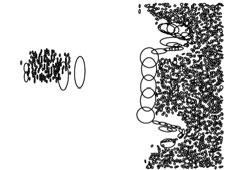
93 Orig. image T1 (Brick) T2 (Carpet) T3 (Chair) T4 (Floor 1) T5 (Floor 2) T6 (Marble) T7 (Wood) (a) Initial labeling of regions (top) vs. the final labeling following relaxation (bottom). Orig. image T1 (Brick) T2 (Carpet) T3 (Chair) T4 (Floor 1) T5 (Floor 2) T6 (Marble) T7 (Wood) (b) Successful segmentation examples. Orig. image T1 (Brick) T2 (Carpet) T3 (Chair) T4 (Floor 1) T5 (Floor 2) T6 (Marble) T7 (Wood) (c) Unsuccessful segmentation examples. Figure 4.6 Segmentation results. 84

94 Animals Our second data set consists of unsegmented images of three kinds of animals: cheetahs, giraffes, and zebras. The training set contains 10 images from each class, and the test set contains 20 images from each class, plus 20 negative images not containing instances of the target animal species. To account for the lack of segmentation, we introduce an additional background class, and each training image is labeled as containing the appropriate animal and the background. Recall from Section that the EM algorithm is initialized with the output of K-means. To initialize K-means on this incompletely labeled data, we randomly assign each feature vector either to the appropriate animal class, or to the background. The ROC curves for each class are shown in Figure 4.7, and segmentation results are shown in Figure 4.8. Overall, our system appears to have learned very good models for cheetahs and zebras, but not for giraffes Cheetah Zebra Giraffe Figure 4.7 ROC curves for the animal dataset. The dashed (resp. solid) line represents performance before (resp. after) relaxation. 85

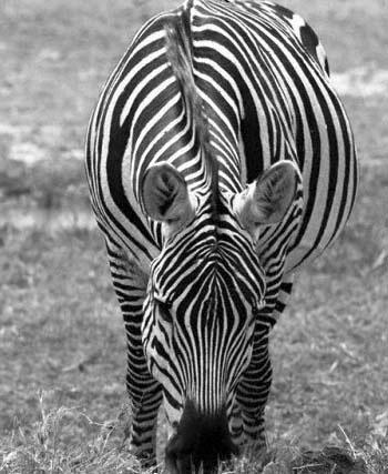
95 Original image Cheetah Zebra Giraffe Background Figure 4.8 Segmentation on the animal dataset. 86

96 We conjecture that several factors account for the weakness of the giraffe model. Some of the blame can be placed on the early stage of feature extraction. Namely, the Laplacianbased affine region detector is not well adapted to the giraffe texture whose blobs have a relatively complex shape. At the learning stage, the system also appears to be distracted by background features, such as sky and trees, that occur more commonly in training samples of giraffes than of the other animals. In the bottom image of Figure 4.8, giraffe-ness is associated with some parts of the background, as opposed to the animals themselves. Part of the problem is that the artificial background class is simply too inhomogeneous to be successfully represented in the mixture framework. A principled solution to this problem would involve partitioning the background into a set of natural classes (e.g., grass, trees, water, rocks, etc.) and building larger training sets that would include these classes in different combinations. Despite somewhat uneven performance, the results presented in this section are promising. Unlike many other methods suitable for modeling natural textures, ours does not require negative examples. The EM framework shows surprising aptitude for automatically separating positive areas of the image from negative ones, without the need for specially designed significance scores such as the ones used by Schmid [137]. 4.3 Discussion The first half of this chapter has presented an approach to texture classification that combines textons and co-occurrence relations using a discriminative maximum entropy framework. While the maximum entropy classifier has proven to be effective for a basic bag-offeatures image representation, augmenting this representation with co-occurrence relations did not produce any improvement. This negative result is echoed in the experiments of Section , where we have observed that, even though relaxation improves the labeling of individual regions, it is not required for effective classification of single-texture images. A 87

97 similar observation was also made by Lu et al. [91] who found that segmenting scenes into their semantic components (or basic material categories) was not necessary for recognizing the scenes as a whole. Interstingly, these findings in the vision literature are consistent with the conventional wisdom in the document classification community, that simple orderless bag-of-words represententations [9, 102, 114] perform best for document classification. It is possible that the whole-image classification task is intrinsically simpler than the region labeling task, and does not require detailed statistical modeling of spatial relations. It is also possible that current image databases are not challenging enough, in that all classes can be distinguished using purely local features. Maybe co-occurrence statistics do not work because existing datasets are too small to allow them to be learned reliably, or maybe stronger spatial relations are needed in order to observe an improvement in performance. These are all interesting questions that the current vision literature has not even begun to address. To investigate them further, it is necessary to conduct larger-scale tests on more difficult texture databases that include a wider variety of classes. The two-stage texture representation framework presented in the second half of this chapter, while showing promise for weakly supervised learning, also has several important shortcomings that should be addressed in subsequent work. Perhaps the most fundamental one is the separation between the two modeling steps of learning the distribution of local appearance and finding the co-occurrence statistics. In particular, the co-occurrence statistics computed during the second step cannot back-propagate to influence the sub-class probability distributions computed in the first step. At testing time, once the posterior probabilities of different sub-class labels have been computed from the generative model of local appearance, the subsequent updates of the probability values no longer depend on the image data. This feature of the relaxation algorithm described in Section is at least partially responsible for the segmentation artifacts present in our results. Our current formulation of co-occurrence relations also has several disadvantages: First, the correlation 88

98 between two neighboring locations depends only on their labels, not on the pixel-level data; and second, correlations between sub-class labels of different textures cannot be estimated reliably in a weakly supervised framework, and must therefore be set by hand. At worst, this can reduce the co-occurrence values to the role of generic smoothness constraints, which blindly enforce continuity in the final segmentation, regardless of the pixel-level evidence. A possible solution to many of the above problems is to represent the image as a conditional random field (CRF) [70, 68]. CRFs provide a principled framework for connecting low-level features with higher-level labels, and for combining local features and relations within the same probabilistic model. The major barrier to adopting CRFs to our problem is the lack (to our knowledge) of efficient learning methods for the weakly supervised setting. This is an extremely challenging problem, one that we hope to address in future research. 89

99 CHAPTER 5 Semi-Local Parts for Object Recognition Achieving true 3D object recognition is one of the most important challenges of computer vision. As a first step towards this goal, it is necessary to develop geometrically invariant object models that can support the identification of object instances in novel images in the presence of viewpoint changes, clutter, and occlusion. This chapter describes an approach to object recognition that represents objects using dictionaries of composite semi-local parts, or geometric configurations of regions that are stable across a range of views of an object, and also across multiple instances of the same object category. We can think of each individual semi-local part as corresponding to an approximated planar and rigid region of the object. For example, the semi-local parts for representing side views of cars shown in Figure 5.1 (a) cover different rigid components (front, back, middle, or just a wheel) that any two given vehicles are likely to share in common. Moreover, because semi-local parts do not have to cover the whole object and can move freely with respect to one another, collections of them are in principle suitable for describing even non-rigid 3D objects, such as the owls in Figure 5.1 (b). The rest of this chapter is organized as follows. Section 5.1 motivates our work, and Section 5.2 describes our weakly supervised procedure for creating dictionaries of semi-local parts for representing multiple object classes. This procedure first performs two-image matching to create candidate parts (Section 5.2.1) and then validates these parts against additional images from positive and negative classes (Section 5.2.2). Section 5.3 presents recognition 90

100 (a) Cars (b) Owls Figure 5.1 Collections of semi-local parts for representing two object classes. The pairs of images that were originally matched to obtain the part are shown one above the other with the matched local features (yellow circles) superimposed. The examples shown here use the scale-invariant local features described in Section and a scale-and-translation alignment model. The aligning transformation between the corresponding groups of features is indicated by the bounding boxes: the axis-aligned box in the top image is mapped onto the parallelogram in the bottom image. (As explained in Section 5.2.1, we use an affine alignment model and then discard any transformation that induces too much distortion.) Note that the boxes are shown for visualization purposes only; they are not required as input to the matching algorithm. 91

101 experiments with affine- and scale-invariant parts (Sections and 5.3.2, respectively). In our recognition experiments, we use two different discriminative models: in Section 5.3.1, where relatively little training data is available, we use a simple voting scheme to classify images according to which class they contain; in Section we work with larger training sets that allow us to learn a maximum entropy classifier that was first introduced in Section 4.1. Finally, the chapter closes with a discussion of several conceptual issues relevant to our approach. The material presented in this chapter has been published in [73, 74]. 5.1 Motivation In recent literature, perhaps the most effective approach to weakly supervised learning of part-based object models is Bayesian [28, 33, 162, 163]. Despite their promise, current Bayesian approaches have substantial shortcomings that limit their applicability to general 3D object recognition. In this chapter, we take aim at two of these shortcomings: lack of geometric invariance and an inefficient strategy for dealing with the correspondence problem. Geometric invariance. To date, the state of the art for Bayesian approaches is scale and translation invariance [33], which means that they are mostly applicable to recognizing fronto-parallel views of upright objects. Unfortunately, while achieving scale invariance already requires a very intricate generative probabilistic framework, a principled probabilistic treatment of rotation or affine invariance is orders of magnitude more complex [78]. Even if one assumes a Gaussian joint distribution on the coordinates of a set of image features, the distribution in the affine-normalized space obtained by expressing all points in the basis given by a reference triple becomes non-gaussian. Moreover, the normalized positions become correlated even if one starts out with uncorrelated errors in individual feature positions. On the other hand, if one assumes a more direct geometric approach to invariance (see, 92

102 e.g., [36]), one gains access to robust and simple methods for computing affine-invariant object representations. The correspondence problem. When attempting unsupervised learning of part-based models, one must inevitably confront the intractable combinatorial problem of determining correspondence, or the assignment of object parts to image regions in the presence of occlusion and clutter. In the typical generative approach to recognition, the Expectation Maximization (EM) algorithm is used for estimating the parameters of probabilistic object models. EM treats correspondence as missing data to be integrated out, which in principle involves computing expectations over the exponentially large space of all possible correspondences, but in practice is usually handled by a variety of approximation techniques. The combinatorics of EM-based learning severely limit the total number of parts in an object model. For example, the system developed by Fergus et al. [33] is, according to its authors, limited to models consisting of up to 6 or 7 parts learned from images containing 20 to 30 features. In turn, this limits both the expressiveness of the corresponding object models and the amount of clutter and/or occlusion that can be tolerated during learning. Perhaps as importantly for us, the missing data approach to correspondence is not satisfying from a philosophical standpoint. For humans, determining correspondence is a crucial step in forming judgments of similarity, which in turn influence such complex cognitive processes as memory and problem solving [43]. For computer vision algorithms, the ability to establish perceptually plausible correspondences is a convincing demonstration of success in the recognition task, one that has yet to be consistently achieved. Therefore, the approach proposed in this chapter is built on the idea that establishing unique correspondence between model and image features (as opposed to averaging over all possible correspondences) is central for successful recognition. 93

103 5.2 Semi-Local Parts For each object class, we construct a dictionary of composite semi-local parts [73], or groups of several nearby regions whose appearance and spatial configuration occurs repeatably in the training set. The key idea is that consistent occurrence of (approximately) rigid groups of simple features in multiple images is very unlikely to be accidental, and must thus be a strong cue for the presence of the object. Note that, unlike the parts used in [1, 28, 33, 162, 163] (points or individual regions), our semi-local parts are not atomic, but are made up of multiple regions, each of which is associated with its own shape (circle or ellipse) and intensity pattern. Making parts composite improves their expressiveness and distinctiveness, and provides a layer of abstraction in representing complex 3D objects. We also propose a direct geometric procedure for learning parts from small collections of input images. Our strategy is to reduce the intractable problem of simultaneous alignment of multiple images to pairwise matching: candidate parts are formed by matching pairs of images, followed by a validation step to discard spurious matches (Figure 5.2). Even though finding optimal correspondence between features in two images is still intractable [46], effective suboptimal solutions can be found using a non-exhaustive constrained search procedure that relies on a number of strong geometric and appearance-based consistency constraints. As a result of these constraints, our matching algorithm is able to return hundreds of candidate parts consisting of a dozen or more features each. Note that the sizes of the parts are not fixed in advance, but are automatically determined by the matching procedure Matching of Pairs of Images As explained above, the fundamental operation in our approach to learning object parts is matching pairs of images from the same class. Algorithm 1 describes our procedure for two-image matching and Figure 5.3 illustrates its major steps. This algorithm is similar to classical alignment search [27, 41, 47, 54], but it uses strong appearance (descriptor similarity) 94

104 Input: Sets of features in two images. Output: A list of candidate parts. for each feature in the first image do Find a list of potential appearance-based matches in the second image. end for Initialize seed groups: for each feature i in the first image and each pair j, k of its neighbors do Enumerate all triples i,j,k in the second image such that i (resp. j, k ) is a potential match of i (resp. j,k) andj, k are neighbors of i (Figure 5.3, top). end for Grow seed groups: for each seed group of matching features do repeat Estimate affine transformation that aligns corresponding features in both images (Figure 5.3, middle). if transformation is geometrically consistent then Align two images using the estimated transformation. Search for additional consistent matches in the neighborhood of existing group. Add these matches to the group (Figure 5.3, bottom). end if until transformation is no longer consistent or no more matches can be found. if current group is larger than a minimum size then Add the group to the list of candidate parts. end if end for Algorithm 1: Two-image matching. For specificity, we give here our affine alignment algorithm, but handling of other transformation models is straightforward (see text). 95

105 Figure 5.2 Our procedure for creating semi-local parts: A candidate part is found by matching two images from the same class and validated by matching against additional training images. constraints to reduce the space of all possible correspondence hypotheses. Initially, for each feature in one image, we create a short list of potential matches in the other image by setting a threshold on descriptor similarity. Then we enumerate all possible seed groups of the smallest size necessary to estimate an aligning transformation between the two images. The most general model considered in our work is affine, for which seed groups consist of triples of matches (Figure 5.3, top). Note, however, that it is straightforward to handle more restricted 2D alignment models, such as scaling or similarity, within the same computational framework. In our implementation, we use linear least squares to estimate an affine alignment between the two groups of regions, and then enforce additional geometric constraints by rejecting any transformation that deviates too much from the desired model. For example, for the scaling-only model used in Section 5.3.2, we reject transformations that include too much skew, rotation, and anisotropic scaling. After estimating an alignment for a given seed group (Figure 5.3, middle), we conduct a greedy search in the same local neighborhood for additional matches satisfying geometric and appearance consistency constraints (Figure 5.3, bottom). Geometric consistency is measured by comparing the shapes of the corresponding features aligned in the same coordinate system. For affine features, we place constraints on the residual of the linear transformations between the centers of the corresponding ellipses, 96

106 j j' i i' image 1 k image 2 Step 1: An initial seed triple. Arrows represent neighborhood constraints and dotted lines represent appearance consistency constraints. k' j j' i i' image 1 k image 2 Step 2: Estimate an affine transformation aligning (i,j,k )with(i, j, k). Features from image 2 mapped onto their corresponding features in image 1 are shown by dashed outlines. k' m j m' j' i l i' l' image 1 k image 2 Step 3: Grow the group by two additional matches that satisfy geometric and appearance consistency constraints. Figure 5.3 Illustration of three steps of Algorithm 1. k' 97

107 as well as on the difference in their orientations and axis lengths. The correspondence search terminates when the alignment is no longer geometrically consistent, or when no further consistent matches can be found. Note that the number of features in the group (the size of the candidate part) is determined automatically as a result. Moreover, since Algorithm 1 generates a large number of seed groups and attempts to grow them all, multiple candidate parts can be returned as a result of just a single matching operation. In the implementation, we use a post-processing step to merge candidate parts that ovelap by a significant amount. The candidate parts returned by the above procedure are (roughly) affinely rigid by construction, i.e., the mapping between two different instances of the same part can be well approximated by a 2D affine transformation. Note that we do not make the overly restrictive assumption that the entire object is planar and/or rigid it is sufficient for the object to possess some (approximately) planar and rigid components. Because of this non-global notion of affine invariance, our method is suitable for modeling rigid 3D objects (Figure 5.4), as well as non-rigid objects such as faces (Figure 5.5). Also refer back to Figure 5.1 for matching examples using scale-invariant features and a scale-and-translation alignment model. In existing literature, similar procedures for growing groups of matches based on geometric and appearance consistency constraints have been successfully applied to the recognition of the same object instance in multiple views [34]; one of the key insights of our work is that such procedures are also quite effective for building models of object classes with substantial intra-class variation. Because of the strong consistency constraints that must be satisfied by semi-local parts, they are much more discriminative than atomic parts, and much less likely to give rise to false detections. Note that our two-image matching procedure can match an image to itself, and is thus directly applicable to the problem of detecting repeated structures and symmetries within a single image [79, 86, 151]. The only change necessary in the implementation is the addition of 98

108 (a) Salt can (b) Shoe (c) Car Figure 5.4 Candidate parts for three 3D objects: (a) a salt can, (b) a shoe, and (c) a car. The two input images to the matching procedure are shown side by side, with the matched ellipses superimposed. For visualization purposes, we also show bounding boxes around the matched ellipses: the axis-aligned box in the left image is mapped onto the parallelogram in the right image by the affine transformation that aligns the matched ellipses. checks to prevent trivial hypotheses that match (almost) every region to itself. A particularly attractive feature of our matching procedure for this application is its ability to discover patterns in substantial amounts of clutter, which is not possible with other, more specialized approaches, e.g., [86]. Figure 5.6 shows the symmetries and repetitions detected in several images. The examples of repetitions detected in the images of fishes and badgers suggest that a single image may be sufficient to construct highly discriminative models for some object categories. This is certainly true for butterflies, which will be used as test subjects in Section

109 (a) Alain Delon (b) Grace Kelly (c) Grace Kelly and Cary Grant Figure 5.5 Candidate parts for face images. (c) Curiously, the face of Grace Kelly in the left image fails to match to her face in the right image, but the matched regions do reveal a structural similarity between her face and Cary Grant s Validation After candidate parts have been formed, they are validated by matching against additional training images. The purpose of validation is to reject spurious parts that arise from clutter and incorrect matching hypotheses. We have experimented with two types of validation: non-discriminative (Section 5.3.1), where a part is only matched against positive images (i.e., images that contain the same object class that was used to generate the candidate part); and discriminative (Section 5.3.2), where a part is matched against both positive and negative images. The latter procedure has the advantage of rejecting parts that occur just as often in non-object images as in object images. For example, a wheel may be a part that occurs in both cars and trucks, and can thus be used in the description of either class, but if we are trying to discriminate between cars and trucks, then the presence of a wheel is not a useful cue. 100

110 (a) Window (b) Totem (c) Badgers (d) Badgers: repetition (e) Fishes: repetition Figure 5.6 Detecting symmetry (top) and repetition (bottom) in single images. In the top images, the axis of reflective symmetry is shown as a dashed line. Note that for the palace window, two different local symmetries are detected. The procedure for detecting a part in a validation image is very similar to two-image matching (Algorithm 1), made simpler and more efficient by the part s relatively small size and (presumed) lack of clutter. A detected instance of a candidate part in a validation image may have multiple features missing because of occlusion, failure of the salient region detector, etc. We define the repeatability of an individual feature within a part as the proportion of detected part instances in positive images in which that feature was present, and refine parts by removing from them all features whose repeatability falls below a certain threshold. Note that in principle, we can use the correspondences between the parts and the positive validation images to further refine the parts by modifying their appearance and shape. At present, we have not implemented this extension because we have generally been satisfied with the quality of parts obtained following validation and removal of spurious features. For each detected instance of a part in a validation image, we define a response score as the number of features in that instance normalized by the total number of features in the part. Next, for each part k and each validation image I, we define a global score ρ k (I) asthe 101

111 Training images Validation score: Figure 5.7 An example of a face part (see Figure 5.12) and its response histograms for discriminative validation. The solid red line (resp. dash-dot blue line) indicates the response histogram for the positive (resp. negative) class. highest response score over all detected instances of part k in that image. This implicitly assumes that an object image can contain at most one instance of each part. In the future, we plan to improve our feature representation to allow for multiple detected instances of the same part. This would allow us to perform more accurate localization for classes such as cars (which have two wheels) or faces (which have two eyes). Finally, note that if part k is not detected in image I at all, we have ρ k (I) =0. For non-discriminative validation, we derive an overall quality measure of a part from its average response score over the validation set, and retain a fixed number of top-scoring parts for each class. For discriminative validation, we compute a quality measure for the part by taking the χ 2 distance between the histograms of part responses over the positive and negative images (see Figure 5.7 for an example). This validation score can range from 1, when the two histograms have no overlap at all, to 0, when they are identical. Just as for non-discriminative validation, a fixed number of highest-scoring parts is retained to represent each class. 102

112 5.2.3 Recognition The part creation, detection, and validation procedures presented so far in this chapter is general in the sense that it can be used with a wide variety of learning and classification schemes. To complete the discussion of our part-based framework, let us briefly sketch the testing or recognition step of our framework while deferring most of the details to our presentation of experimental results in Section 5.3. Given a novel test image I, we perform the detection procedure for each part k from the dictionary, and, just as during the validation step, record the response score ρ k (I) of this part for this image. Next, our goal is to decide which object instance is present in the image based on the vector of response scores for all parts. In the experiments, we use several ways of accomplishing this goal. In Section 5.3.1, we simply let each part vote for the class it represents with its response score, and assign the test image to the class with the highest cumulative vote. While this approach is somewhat ad-hoc, it does not require a separate step of training a discriminative model over the response scores, and therefore it works well in situations when very few training images are available. On the other hand, in Section 5.3.2, we work with larger datasets, and we are able to train two classifiers. The first is a Naive Bayes classifier that works by estimating P (ρ k c), the probability distributions of response scores for each part k given that the image contains an object of class c. The second is the maximum entropy classifier first described in Section 4.1 that uses feature functions based on individual response scores as well as on the overlap between pairs of parts. Details of these feature functions and our training protocol will be further discussed in Section Recognition Experiments This section demonstrates the promise of our approach with recognition experiments on three datasets. Section presents results on a dataset consisting of seven classes of butterflies. The large amount of geometric variability in this dataset requires us to use 103

113 Admiral Swallowtail Machaon Monarch 1 Monarch 2 Peacock Zebra Figure 5.8 The butterfly dataset. Three samples of each of the seven classes are shown. Monarch 1 and 2 are the same butterfly species with wings closed and open, respectively. This database is publicly available at grp/data. a full affine alignment model. Section considers two datasets that have wider intraclass appearance variability, but a narrower range of geometric variation that can be handled with a scale-and-translation alignment model. The first is a four-class subset of Caltech6 [33] consisting of airplanes, cars, faces, and motorbikes; and the second is a dataset consisting of six species of birds Affine-Invariant Parts In this section, we report results for multi-class recognition as well as binary detection on a dataset composed of 619 images of butterflies collected from the Internet. Seven butterfly classes are represented (see Figure 5.8 for sample images of each). The dataset is extremely diverse, with pictures varying widely in terms of size and quality (motion blur, lack of focus, resampling and compression artifacts are among the factors affecting quality). From one viewpoint, butterflies may be considered pretty toy subjects for testing the descriptive power of our local affine models, since the geometry of a butterfly is locally planar for each wing (though usually not globally planar). In addition, the species identity of a butterfly is 104

114 determined by a basically stable geometric wing pattern, though appearance can be significantly affected by individual variations, lighting, and imaging conditions. But from another viewpoint, recognizing butterflies is a challenging task. For one, a typical butterfly part is sufficiently complex to require at least a dozen features to be discriminative, which is beyond the range of most of the current state-of-the-art recognition systems [1, 28, 33, 162, 163]. Moreover, the levels of invariance (translation and scale) possessed by existing algorithms are clearly insufficient for recognizing insects in natural imagery. In our dataset, butterflies appear in highly cluttered environments, with most images containing on the order of a thousand local features. For the experiments of this section, we perform feature extraction using the affine-adapted Laplacian detector. We chose this detector over the Harris because it tends to find regions that are centered away from object boundaries and because blobs are clearly salient for butterflies, whose wing patterns feature spots and stripes. As in Section 3.1, we use SPIN and RIFT descriptors to compare regions. Note that the RIFT descriptor as originally introduced in that section is not invariant to reflection of the normalized patch. Unlike in our texture recognition work, we require reflection invariance for finding semi-local parts. Reflection of the normalized patch reverses the order of directions in the histogram of gradient orientations within each circular subregion of the RIFT descriptor. Thus, when finding the distance between two RIFT descriptors, we simply take the minimum over both orders. One other issue is how to combine SPIN and RIFT descriptors in determining the appearance-based dissimilarity or matching score between two patches. We set the matching score to be the minimum of the Euclidean distances between the two spin images or RIFT descriptors (note that both descriptors are normalized to have zero mean and unit norm, thus Euclidean distances between them lie in the same range and are comparable). Empirically, this approach performs better than other ways of combining descriptors, since it provides robustness against instabilities in region extraction and intensity normalization. The descriptors (particularly 105

115 Class Part size Test images Correct (rate) Admiral 179 (12/28) (0.871) Swallowtail 252 (18/29) (0.750) Machaon 148 (12/21) (0.965) Monarch (14/67) (0.729) Monarch (19/36) (0.914) Peacock 102 (8/14) (1.000) Zebra 209 (16/31) (0.892) Total (0.904) Table 5.1 Classification results for the butterflies. The second column shows the total part size for each class (the sum of sizes of individual parts), and the size of the smallest and the largest parts are listed in parentheses. For this database, the kernel-based bag-of-features method of Section 3.2 achieved 87% accuracy, below our rate of 90.4%. spin images) can be sensitive to transformations of the intensity values (i.e., noise, JPEG compression, sharpening) and to shifts in the position of the center of the normalized patch, so a large distance between two spin images or two RIFT descriptors is not always a reliable indication of perceptual difference. Thus, in determining the matching score between two patches, it makes sense to trust the descriptor that produces the lower distance. For modeling, 16 images from each class were chosen at random. Candidate parts were formed by matching between eight pairs (an alternative approach would have been to match every possible pair of images in the training set, but this did not prove necessary, as sufficient numbers of candidate parts were obtained from the eight pairs). Ten positive verification images were used for each class to remove unstable regions and to rank parts according to their non-discriminative validation score. Top ten parts were retained and used for recognition. Multi-class classification is performed as follows. First, the parts for all classes are detected in each training image. Though multiple instances of the same part may be found, we 106

116 Classification rate Number of parts 8 10 Figure 5.9 Classification rate vs. number of parts. retain only the single instance with highest absolute response score, or the number of detected features. The cumulative score for a given class is given by the relative response of all its parts, or the total number of features detected in all parts divided by the sum of part sizes. Each image is assigned to the class having the maximum relative response score. Table 5.1 shows classification results obtained using the above approach. Our overall classification rate is 90.4%. This is higher than the baseline rate of 87% obtained with the kernel-based bag-offeatures method of Section 3.2 using rotation-invariant (H+L)(SPIN+SIFT) features. 1 Note that our relative response score tends to favor classes with smaller part size, as larger parts tend to be much looser than smaller ones: that is, the fraction (though not the absolute number) of regions they pick up tends to be smaller. Figure 5.9 shows how the performance of our system is affected by using different numbers of parts for classification. Though the classification rate is already respectable with just a single part, using multiple parts is clearly important for improving performance. 1 Several feature combinations and levels of invariance were tested, and the feature combination reported here is the one that obtained the highest performance. 107

117 (a) Part w/ highest validation score (b) Detection examples (c) ROC curves Peacock Monarch 2 Monarch 1 Machaon Swallowtail Admiral Part size: (0.64) Part size: 27 7 (0.26) Part size: (0.55) Part size: (0.27) Part size: (0.42) Part size: 12 6 (0.50) (0.871) (0.938) (0.930) (0.938) (0.948) (0.870) (0.938) Zebra Part size: (0.45) Figure 5.10 Butterfly modeling and detection. (a) The part with the highest validation score for each class. (b) Example of detecting the part from (a) in a single test image. Detected regions are shown in yellow and occluded ones are reprojected from the model in blue. The total number of detected features (absolute response) and the corresponding relative response are shown below each image. Note that the correspondences for the swallowtail and zebra are incorrect. (c) ROC curves for detection. Three thresholds for relative response (0.33, 0.5, 0.66) are marked on the curve. The dark square marks the ROC equal error rate, which is listed in parentheses next to the threshold value at at which it is attained. 108

118 We can get an alternative assessment of performance by considering the binary detection task, where for each image and each class, we ask whether an instance of the from this class is present. This decision can be made by setting a threshold on the relative response score. By considering all possible thresholds, we get an ROC curve, a plot of the true positive rate (the number of correct positives detected over the total number of positives for the class) vs. the false positive rate (the number of false positives over the total number of negatives in the dataset). These curves, given in Figure 5.10, also show the ROC equal error rate for each class. This is the true positive rate that is equal to one minus the false positive rate. The equal error rates achieved by our system are high, showing that detection can indeed be performed successfully Scale-Invariant Parts This section presents recognition results obtained on two multi-class object databases. The first is a subset of the publicly available CalTech database [33], which we have already used in Section 3.2. We have taken 300 images each from four classes: airplanes, rear views of cars, faces, and motorbikes (for examples of Caltech images, refer back to Figure 3.13). The second database, which we collected from the Web, consists of 100 images each of six different classes of birds: egrets, mandarin ducks, snowy owls, puffins, toucans, and wood ducks (Figure 5.11). Because these databases mostly feature objects in canonical poses (i.e., upright heads, frontal or side views of birds), they do not require the full affine alignment model; scale with translation are sufficient. For our texture recognition experiments of Chapter 3 and butterfly experiments of Section 5.3.1, Laplacian region detectors have proven to be successful, since most of the classes in these experiments could be characterized quite well by salient blob-like features. However, we have found Laplacian features to be much less repeatable for classes with complex internal structures, e.g., eyes, wheels, heads, etc. Instead, in this section we extract salient regions 109

119 Egret Mandarin duck Snowy Owl Puffin Toucan Wood duck Birds database Figure 5.11 Three examples from each class of the birds database. This database is publicly available at grp/data. using the scale-invariant detector of Jurie and Schmid [61], which finds salient circular configurations of edge points, and is robust to clutter and texture variations inside the regions. Just as in Section 4.1.2, the appearance of the extracted regions is represented using SIFT descriptors. For the Caltech database, 50 randomly chosen images per class are used for creating candidate parts. Each image is paired up to two others, for a total of 100 initialization pairs. Of the several hundred candidate parts yielded by this matching process, the 50 largest ones undergo discriminative validation. Specifically, these candidate parts are matched against every image from the validation set, which also contains 50 randomly chosen images per class, and 20 highest-scoring parts per class are retained to form the part dictionary. Finally, the remaining 200 images per class make up the test set. We follow the same protocol for the bird dataset, except that 20 images per class are used for finding candidate parts, another 30 for validation, and the remaining 50 for testing. Figures 5.12 and 5.13 illustrate training and validation (part selection). As can be seen from the plots of validation scores for all selected parts, the quality of part dictionaries found for different classes varies widely. Extremely stable, repeatable parts are formed for faces, 110

120 Top part Validation hist. Top 20 scores (a) (b) (c) Score Planes size Part number score Score Cars size Part number score Score Faces size Part number score Score Bikes size Part number score Figure 5.12 Learning part vocabularies for the CalTech database. (a) The highest-scoring part for each class. (b) Response histograms for the top part. The solid red line (resp. dashed blue line) indicates the histogram of response scores of the part in all positive (resp. negative) training images. Recall that the validation score of the part is given by the χ2 distance between the two histograms. (c) Plots of top 20 part scores following validation. 111

121 Top part Validation hist. Top 20 scores (a) (b) (c) Score 0.6 Egret size Part number score Score Mandarin size Part number score Score Snowy owl size Part number score Score Puffin size Part number score Score Toucan size Part number score Wood duck Score size Part number score Figure 5.13 Learning part vocabularies for the birds database. (a) The highest-scoring part for each class superimposed on the two original training images. (b) Validation response histograms for the top parts. (c) Validation scores for the top 20 parts from each class. 112

122 motorbikes, and ducks. The classes with the weakest parts are airplanes for the CalTech database and egrets for the bird database. Both airplanes and egrets lack characteristic texture, and often appear against busy backgrounds that generate a lot of detector responses (buildings, people, and airport machinery in case of planes, or grass and branches in case of egrets). In addition, both egrets and airplanes are thin objects, so the local regions that overlap the object also capture a lot of background. Thus, the SIFT descriptors computed over these regions end up describing mostly clutter. To alleviate this problem, we plan to experiment with alternative descriptors that capture the shape of the edges close to the boundary of the scale-invariant regions [61], as opposed to the internal texture, as the SIFT descriptor does. Note that our part selection framework is suitable for choosing between semi-local parts based on different descriptors, since it abstracts from the low-level details of matching (i.e., how appearance similarity is computed, what aligning transformation is used, or how the correspondence search is performed), and looks only at the end result of the matching on the training set (i.e., how repeatable the resulting parts are, and whether they can be used to distinguish between positive and negative examples for a given class). The parts obtained for classes other than airplanes and egrets have higher scores and capture much more salient object features. Interestingly, though, for cars, even the highestscoring part includes spurious background detections along the horizontal line at the eye level of the image. This comes from the relative visual monotony of the car class: all the rear views of cars were apparently captured through the windshield by a person in the front seat. Thus, the horizon formed by the converging sides of the road is approximately in the same location in all the images, and the scenery at the roadside (trees, buildings) gives rise to a lot of features in stable positions that are consistently picked up by the matching procedure. In this section, we use the discriminative maximum entropy framework introduced in Section to build a principled probabilistic model for object recognition. Recall from 113

123 Section that the use of the maximum framework requires us to define a set of feature functions for each class. For each part k and each training image I, we compute a normalized feature function based on its response score ρ k (I) as defined in Section 5.2.2: g k (I) = ρ k(i) k ρ k (I). Feature function values computed on images from the validation set are used as training data to estimate the parameters of the exponential model. Just as in the texture recognition experiments of Section 4.1, we also investigate whether, and to what extent, incorporating relations into the object representation improves classification performance. To this end, we define overlap relations between pairs of parts that belong to the same class. Let ω k,l (I) be the overlap between detected instances of parts k and l in the image I, i.e., the ratio of the intersection of the two parts to their union. This ratio ranges from 0 (disjoint parts) to 1 (coincident parts). Then we define g k,l (I) = ω k,l (I) k,l ω k,l (I). The overlap relations are very flexible in effect, they enforce only spatial coherence. This flexibility potentially allows us to deal with non-rigid and/or articulated objects. In the future, we plan to experiment with more elaborate relations that take into account the distance, relative scale, or relative orientations of the two parts [1]. Finally, it is important to note that we currently do not use feature selection techniques to reduce the number of overlap relations within the exponential model. Because of the small size of the part dictionaries used in the experiments presented in the next section (namely, 20 parts per class), the resulting number of overlap relations (190 per class) is quite manageable, unlike in the texture recognition experiments of Section 4.1, where we had to contend with millions of potential co-occurrence relations. Tables 5.2 and 5.3 show classification performance of several methods with 20 parts per class. The first column of the tables shows the performance of a baseline Naive Bayes 114

124 CalTech Naive Exp. Exp. Exp. parts & database Bayes parts relations relations Airplanes Cars (rear) Faces Motorbikes All classes Table 5.2 Classification rates for the CalTech database using 20 parts per class. approach with likelihood given by P (I c) = k P (ρ k (I) c). The distributions P (ρ k c) are found by histogramming the response scores of part k on all training images from class c. Note that we take into account the responses of parts on images from all classes, not only the class which they describe. Roughly speaking, we expect P (ρ k (I) c) tobehighifpartk describes class c and ρ k (I) is high, or if part k does not describe class c and ρ k (I) is low or zero. Thus, to conclude that an object from class c is present in the image, we not only have to observe high-response detections of parts from class c, but also low-response detections of parts from other classes. The exponential model, which encodes the same information in its feature functions, also uses this reasoning. The second (resp. third, fourth) columns of Tables 5.2 and 5.3 show the classification performance obtained with exponential models using the g k features only (resp. the g k,l only, g k and g k,l combined). For the CalTech database, the Naive Bayes and the exponential parts-only models achieve very similar results, though under the exponential model, airplanes have a lower classification rate, which is intuitively more satisfying given the poor part dictionary for this class. Note that our classification accuracy of over 96% on the four CalTech classes is comparable to other recently published results [20, 23]. For the bird database, the 115

125 Birds Naive Exp. Exp. Exp. parts & database Bayes parts relations relations Egret Mandarin Snowy owl Puffin Toucan Wood duck All classes Table 5.3 Classification rates for the birds database using 20 parts per class. For this database, the kernel-based bag-of-features method of Section 3.2 achieved 83% accuracy, below our best result of 92.33%. exponential model outperforms Naive Bayes. Moreover, our best classification rate of 92.33% is higher than the best rate of 83% obtained with the kernel-based bag-of-features method of Section 3.2 using scale-invariant (H+L)(SIFT) features. For both databases, relations-only features alone perform considerably worse than the parts-only features, and combining partsbased with relation-based features brings no improvement. Figure 5.14 shows a plot of the classification rate for the exponential model as a function of part dictionary size. Note that the curves are not monotonic adding a part to the dictionary can decrease performance. This behavior may be an artifact of our scoring function for part selection, which is not directly related to classification performance. In the future, we plan to experiment with part selection based on increase of likelihood under the exponential model [6]. Though we did not conduct a quantitative evaluation of localization accuracy, the reader may get a qualitative idea by examining Figures 5.15 and 5.16, which show examples of part detection on several test images. A poorer part vocabulary for a class tends to lead to poorer localization quality, though this is not necessarily reflected in lower classification 116

126 Recognition rate relations only parts only parts and relations Parts per class Recognition rate relations only parts only parts and relations Parts per class Figure 5.14 Classification rate (exp. parts) as a function of dictionary size: CalTech database (left), birds database (right). For the CalTech database, because three of the four classes have extremely strong and redundant parts, performance increases very little as more parts are added. For the bird database, diminishing returns set in as progressively weaker parts are added. rates. Specifically, an object class represented by a relatively poor part vocabulary may still achieve a high classification rate, provided that parts for other classes do not generate too many false positives on images from this class. The airplane example in Figure 5.15 (b) is a good illustration of this phenomenon: only three airplane parts are detected in this image, yet the airplane is recognized correctly since the image does not contain enough clutter to generate false detections of parts from other classes. Somewhat frustratingly, we have found that inter-part relations do not improve recognition performance. This is consistent with the findings of Section 4.1, where texton cooccurrence relations also did not improve the accuracy of maximum entropy texture classification. From examining the part detection examples in Figures 5.15 and 5.16, it seems intuitively clear that the pattern of overlap of different part instances encodes useful information: the part detections that lie on the object tend to be clustered close together, while false detections are frequently scattered all over the image. We currently conjecture that the 117

127 Successfully classified images (b) (c) Bikes Faces Cars Planes (a) Misclassified image Figure 5.15 CalTech results. (a), (b) Two examples of correctly classified images per class. Left of each column: original image. Right of each column: transformed bounding boxes of all detected part instances for the given class superimposed on the image. (c) Examples of misclassified images. Note that localization is poor for airplanes and very good for faces (notice the example a changed facial expression). For motorbikes, the front wheel is particularly salient. Out of the entire test set, only one bike image was misclassified, and in it the front wheel is not properly visible. overlap information may be more useful for localization than for recognition. In the future, we plan to evaluate localization quantitatively. 5.4 Discussion In this chapter, we have presented a weakly supervised framework for modeling 3D objects in terms of geometrically invariant semi-local parts. The two-image matching procedure that forms the core of our method is also applicable to identifying repeated structures and symmetries within a single image an interesting application which today is rarely treated 118

128 Successfully classified images (b) (c) Wood duck Toucan Puffin Owl Mandarin Egret (a) Misclassified image Figure 5.16 Birds database results. (a), (b) Two examples of successfully classified images per class. The original test image is on the left, and on the right is the image with superimposed bounding boxes of all detected part instances for the given class. Notice that localization is fairly good for mandarin and wood ducks (the head is the most distinctive feature). Though owl parts are more prone to false positives, they do capture salient characteristics of the class: the head, the eye, and the pattern of the feathers on the breast and wings. (c) Misclassified examples. The wood duck class has no example because it achieved 100% classification rate. 119

129 in the same context as recognition (see [85] for a model-based recognition approach that takes advantage of symmetries). For our primary goal of 3D object recognition, the proposed approach has the advantages of robustness and flexibility. Namely, it is capable of learning multiple variable-sized parts from images containing a significant amount of noise and clutter. The promise of our part-based method is also demonstrated by its ability to outperform the bag-of-features method of Chapter 3 on our butterfly and bird databases. We conclude this presentation with a discussion of several conceptual issues relevant to our work. Alignment. The search algorithm described in Section is reminiscent of the alignment techniques used in model-based vision [27, 41, 47, 54]. While the process of detecting an existing part in a test image may indeed be thought of as alignment (albeit using a novel representation based on constellations of local features), our overall modeling approach is not. Whereas in classical alignment globally rigid models are built manually and/or from segmented images, our method is capable of handling unsegmented, heavily cluttered input. Another key departure from classical alignment is that our algorithm does not seek a global transformation between two images, nor does it assume that the object being modeled is either planar and/or globally rigid. Instead, we exploit the fact that smooth surfaces are planar in the small, and that local affine models are sufficient to handle large viewpoint variations for approximately coplanar, close-by patches, as well as small non-rigid transformations of the layout of these patches. Because the part model is local, it is also robust to large global deformations. Training set size. Our procedure for learning semi-local parts requires just a pair of images for candidate part creation, and a relatively small number (up to thirty) for validation. Recently, it has been observed that very few training images are actually necessary for learning object models provided the learner is equipped with a good prior on the parameters of the model [28]. In our case, the prior is the strong notion of visual similarity, making it possible to learn part-based models from extremely small training sets. 120

130 Modeling the background. Many previous approaches to object detection, whether classifier-based (discriminative) [1] or probabilistic (generative) [28, 33, 162, 163], require an explicit model of the background. However, we believe that the notion of modeling the background is problematic, since intuitively, it is much harder to describe the concept of the complement of the class of interest than the class itself. By contrast, our approach completely avoids the necessity of modeling the background by virtue of its reliance on strong geometric consistency constraints. In our work, the background is implicitly assumed to be non-repeatable, an assumption that sometimes fails for extremely small sets of images, necessitating the use of the validation procedure. Inter-part relations. The most important negative result of this chapter is the lack of performance improvement from overlap relations in Section Recall that we have observed the same behavior for textons-and-relations models in Section 4.1. For object recognition, the lack of improvement can be ascribed, at least partly, to the weakness of our overlap relations, especially compared to the strong geometric consistency constraints encoded within semi-local parts. In the future, we plan to investigate geometric relations that capture more discriminative information, and to test their behavior for classification on additional object databases. 121

131 CHAPTER 6 Spatial Pyramid Matching for Scene Recognition In this chapter, we consider the problem of recognizing the semantic category of an image. For example, we may want to classify a photograph as depicting a scene (forest, street, office, etc.) or as containing a certain object of interest. As a solution to this problem, we propose a global non-invariant scene representation based on aggregating statistics of local features over fixed subregions and a kernel-based recognition method that computes a rough geometric correspondence using an efficient approximation technique adapted from the pyramid matching scheme of Grauman and Darrell [45]. Our method involves repeatedly subdividing the image and computing histograms of local features at increasingly fine resolutions. As shown by experiments in Section 6.4, this simple operation suffices to significantly improve performance over a basic bag-of-features representation, and even over methods based on detailed geometric correspondence. The research presented in this chapter has been published in [76]. 6.1 Motivation Previous research has shown that statistical properties of the scene considered in a holistic fashion, without any analysis of its constituent objects, yield a rich set of cues to its semantic category [117]. Our own experiments confirm that global representations can be surprisingly effective not only for identifying the overall scene, but also for categorizing images as containing specific objects, even when these objects are embedded in heavy clutter 122

132 and vary significantly in pose and appearance. This said, we do not advocate the direct use of a global method for object recognition (except for very restricted sorts of imagery). Instead, we envision a subordinate role for this method. It may be used to capture the gist of an image [150] and to inform the subsequent search for specific objects (e.g., if the image, based on its global description, is likely to be a highway, we have a high probability of finding a car, but not a toaster). In addition, the simplicity and efficiency of our proposed method, in combination with its tendency to yield unexpectedly high recognition rates on seemingly challenging data, could make it a good baseline for calibrating newly acquired datasets and for evaluating more sophisticated recognition approaches. In computer vision, histograms have a long history as a method for image description (see, e.g., [136, 146]). Koenderink and Van Doorn [66] have generalized histograms to locally orderless images, or histogram-valued scale spaces (i.e., for each Gaussian aperture at a given location and scale, the locally orderless image returns the histogram of image features aggregated over that aperture). Our spatial pyramid approach can be thought of as an alternative formulation of a locally orderless image, where instead of a Gaussian scale space of apertures, we define a fixed hierarchy of rectangular windows. Koenderink and Van Doorn have argued persuasively that locally orderless images play an important role in visual perception. Our retrieval experiments (Figure 6.4) confirm that spatial pyramids can capture perceptually salient features and suggest that locally orderless matching may be a powerful mechanism for estimating overall perceptual similarity between images. It is important to contrast our proposed approach with multiresolution histograms [48], which involve repeatedly subsampling an image and computing a global histogram of pixel values at each new level. In other words, a multiresolution histogram varies the resolution at which the features (intensity values) are computed, but the histogram resolution (intensity scale) stays fixed. We take the opposite approach of fixing the resolution at which the features are computed, but varying the spatial resolution at which they are aggregated. 123

133 This results in a higher-dimensional representation that preserves more information (e.g., an image consisting of thin black and white stripes would retain two modes at every level of a spatial pyramid, whereas it would become indistinguishable from a uniformly gray image at all but the finest levels of a multiresolution histogram). Finally, unlike a multiresolution histogram, a spatial pyramid, when equipped with an appropriate kernel, can be used for approximate geometric matching. The operation of subdivide and disorder i.e., partition the image into subblocks and compute histograms (or histogram statistics, such as means) of local features in these subblocks has been practiced numerous times in computer vision, both for global image description [44, 147, 150] and for local description of interest regions [89]. Thus, though the operation itself seems fundamental, previous methods leave open the question of what is the right subdivision scheme (although a regular 4 4 grid seems to be the most popular implementation choice), and what is the right balance between subdividing and disordering. The spatial pyramid framework suggests a possible way to address this issue namely, the best results may be achieved when multiple resolutions are combined in a principled way. It also suggests that the reason for the empirical success of subdivide and disorder techniques is the fact that they actually perform approximate geometric matching. 6.2 Spatial Pyramid Matching We first describe the original formulation of pyramid matching [45], and then introduce our application of this framework to create a spatial pyramid image representation Pyramid Match Kernels Let X and Y be two sets of vectors in a d-dimensional feature space. Grauman and Darrell [45] propose pyramid matching to find an approximate correspondence between these two sets. Informally, pyramid matching works by placing a sequence of increasingly coarser 124

134 grids over the feature space and taking a weighted sum of the number of matches that occur at each level of resolution. At any fixed resolution, two points are said to match if they fall into the same cell of the grid; matches found at finer resolutions are weighted more highly than matches found at coarser resolutions. More specifically, we construct a sequence of grids at resolutions 0,...,L, such that the grid at level l has 2 l cells along each dimension, for a total of D =2 dl cells. Let H l X and Hl Y denote the histograms of X and Y at this resolution, so that HX l (i) andhl Y (i) are the numbers of points from X and Y that fall into the ith cell of the grid. Then the number of matches at level l is given by the histogram intersection function [146]: I(H l X,H l Y )= D min ( HX(i),H l Y l (i) ). (6.1) i=1 In the following, we will abbreviate I(H l X,Hl Y )toil. Note that the number of matches found at level l also includes all the matches found at the finer level l + 1. Therefore, the number of new matches found at level l is given by I l I l+1 1 for l =0,...,L 1. The weight associated with level l is set to,whichis 2 L l inversely proportional to cell width at that level. Intuitively, we want to penalize matches found in larger cells because they involve increasingly dissimilar features. Putting all the pieces together, we get the following definition of a pyramid match kernel: κ L (X, Y ) = I L + L 1 l=0 = 1 2 L I L l ( I l I l+1) (6.2) L l=1 1 2 L l+1 Il. (6.3) Both the histogram intersection and the pyramid match kernel are Mercer kernels [45] Spatial Matching Scheme As introduced in [45], a pyramid match kernel works with an orderless image representation. It allows for precise matching of two collections of features in a high-dimensional 125

135 appearance space, but discards all spatial information. This chapter advocates an orthogonal approach: perform pyramid matching in the two-dimensional image space, and use traditional clustering techniques in feature space. 1 Specifically, we quantize all feature vectors into M discrete types, and make the simplifying assumption that only features of the same type can be matched to one another. Each channel m gives us two sets of twodimensional vectors, X m and Y m, representing the coordinates of features of type m found in the respective images. The final kernel is then the sum of the separate channel kernels: K L (X, Y )= M κ L (X m,y m ). (6.4) m=1 This approach has the advantage of maintaining continuity with the popular visual vocabulary paradigm in fact, it reduces to a standard bag of features when L =0. Because the pyramid match kernel (6.3) is simply a weighted sum of histogram intersections, and because c min(a, b) =min(ca, cb) for positive numbers, we can implement K L as a single histogram intersection of long vectors formed by concatenating the appropriately weighted histograms of all channels at all resolutions (Figure 6.1). For L levels and M channels, the resulting vector has dimensionality M L l=0 4l = M 1 3 (4L+1 1). Several experiments reported in Section 6.4 use the settings of M = 400 and L = 3, resulting in dimensional histogram intersections. However, these operations are efficient because the histogram vectors are extremely sparse (in fact, just as in [45], the computational complexity of the kernel is linear in the number of features). It must also be noted that we did not observe any significant increase in performance beyond M = 200 and L = 2, where the concatenated histograms are only 4200-dimensional. The final implementation issue is that of normalization. For maximum computational efficiency, we normalize all histograms by the total weight of all features in the image, in effect forcing the total number of features in all images to be the same. Because we use a 1 In principle, it is possible to integrate geometric information directly into the original pyramid matching framework by treating image coordinates as two extra dimensions in the feature space. 126

136 + + level level level w 0 w 1 w 2 Figure 6.1 Toy example of constructing a three-level pyramid. The image has three feature types, indicated by circles, diamonds, and crosses. At the top, we subdivide the image at three different levels of resolution. Next, for each level of resolution and each channel, we count the features that fall in each spatial bin. Finally, we weight each spatial histogram according to eq. (6.3). dense feature representation (see Section 6.3), and thus do not need to worry about spurious feature detections resulting from clutter, this practice is sufficient to deal with the effects of variable image size. 6.3 Feature Extraction This section briefly describes the two kinds of features used in the experiments of Section 6.4. First, we have so-called weak features, which are oriented edge points, i.e., points whose gradient magnitude in a given direction exceeds a minimum threshold. We extract edge points at two scales and eight orientations, for a total of M = 16 channels. We 127

137 designed these features to obtain a representation similar to the gist [150] or to a global SIFT descriptor [89] of the image. For better discriminative power, we also utilize higher-dimensional strong features based on local image patches. In all the experiments presented in the previous chapters of this dissertation, we derived our image representations from the output of salient feature detectors. However, in this chapter, instead of using Harris or Laplacian interest points we simply sample fixed-size patches on a regular grid. Intuitively, we need features on a dense grid in order to capture uniform regions such as sky, calm water, or road surface regions that do not generate any interest point detections, but are very important for forming complete descriptions of natural scenes. Indeed, Fei-Fei and Perona [30] have shown that regular grids work better for scene classification then interest points. Also note that our target application of scene recognition does not require local features to be geometrically invariant, since imaging conditions for landscape and indoor photographs are usually fairly stable (i.e., the camera is assumed to be distant from the objects in the scene, and its orientation is usually upright), whereas the sources of within-class variability for natural scene categories are so diverse and complex that they cannot be compensated by invariance to simple local 2D image transformations. In the experiments presented in Section 6.4, our grid spacing is 8pixelsandpatchsizeis We represent the appearance of the patches using SIFT descriptors, and perform k-means clustering of a random subset of patches from the training set to form a visual vocabulary. Typical vocabulary sizes for our experiments are M = 200 and M = Experiments In this section, we report results on three diverse datasets: fifteen scene categories [30], Caltech101 [29], and Graz [118]. Recall that the last two datasets were used in the evaluation of Section 3.2; in this section, we will be able to compare the results of our spatial pyramid 128

138 method to the results obtained by the bag-of-features method of Chapter 3. As is the case for all the experiments presented in this dissertation, we perform all processing in grayscale, even when color images are available. All experiments are repeated ten times with different randomly selected training and test images, and the average of per-class recognition rates 2 is recorded for each run. The final result is reported as the mean and standard deviation of the results from the individual runs. Multi-class classification is done with a support vector machine (SVM) trained using the one-versus-all rule: a classifier is learned to separate each class from the rest, and a test image is assigned the label of the classifier with the highest response Scene Category Recognition Our first dataset (Figure 6.2) is composed of fifteen scene categories: thirteen were provided by Fei-Fei and Perona [30] (eight of these were originally collected by Oliva and Torralba [117]), and two (industrial and store) were collected by us. Each category has 200 to 400 images, and average image size is pixels. The major sources of the pictures in the dataset include the COREL collection, personal photographs, and Google image search. This is probably the most complete scene category dataset used in the literature thus far, though the low resolution of its images is somewhat of a disadvantage. Table 6.1 shows detailed results of classification experiments using 100 images per class for training and the rest for testing (the same setup as [30]). First, let us examine the performance of strong features for L =0andM = 200, corresponding to a standard bag of features. Our classification rate is 72.2% (74.7% for the 13 classes inherited from Fei- Fei and Perona), which is much higher than their best results of 65.2%, achieved with an orderless method and a feature set comparable to ours. We conjecture that Fei-Fei and Perona s approach is disadvantaged by its reliance on latent Dirichlet allocation (LDA) [9], 2 The alternative performance measure, the percentage of all test images classified correctly, can be biased if test set sizes for different classes vary significantly. This is especially true of the Caltech101 dataset, where some of the easiest classes are disproportionately large. 129

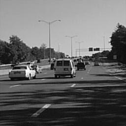
139 office kitchen living room bedroom store industrial tall building inside city street highway coast open country mountain forest suburb Figure 6.2 Example images from the scene category database. The starred categories originate from Oliva and Torralba [117], the industrial and store categories were collected by us, and the remaining ones are from Fei-Fei and Perona [30]. Weak features (M = 16) Strong features (M = 200) Strong features (M = 400) L Single-level Pyramid Single-level Pyramid Single-level Pyramid 0(1 1) 45.3 ± ± ± 0.3 1(2 2) 53.6 ± ± ± ± ± ± 0.5 2(4 4) 61.7 ± ± ± ± ± ± 0.5 3(8 8) 63.3 ± ± ± ± ± ± 0.6 Table 6.1 Classification results for the scene category database (see text). results for each kind of feature are shown in bold. The highest 130

140 which is essentially an unsupervised dimensionality reduction technique and as such, is not necessarily conducive to achieving the highest classification accuracy. To verify this, we have experimented with probabilistic latent semantic analysis (plsa) [52], which attempts to explain the distribution of features in the image as a mixture of a few scene topics or aspects and performs very similarly to LDA in practice [143]. Following the scheme of Quelhas et al. [122], we run plsa in an unsupervised setting to learn a 60-aspect model of half the training images. Next, we apply this model to the other half to obtain probabilities of topics given each image (thus reducing the dimensionality of the feature space from 200 to 60). Finally, we train the SVM on these reduced features and use them to classify the test set. In this setup, our average classification rate drops to 63.3% from the original 72.2%. For the 13 classes inherited from Fei-Fei and Perona, it drops to 65.9% from 74.7%, which is now very similar to their results. Thus, we can see that latent factor analysis techniques can adversely affect classification performance, which is also consistent with the results of Quelhas et al. [122]. Next, let us examine the behavior of spatial pyramid matching. For completeness, Table 6.1 lists the performance achieved using just the highest level of the pyramid (the singlelevel columns), as well as the performance of the complete matching scheme using multiple levels (the pyramid columns). For all three kinds of features, results improve dramatically as we go from L = 0 to a multi-level setup. Though matching at the highest pyramid level seems to account for most of the improvement, using all the levels together confers a statistically significant benefit. For strong features, single-level performance actually drops as we go from L =2toL = 3. This means that the highest level of the L = 3 pyramid is too finely subdivided, with individual bins yielding too few matches. Despite the diminished discriminative power of the highest level, the performance of the entire L = 3 pyramid remains essentially identical to that of the L = 2 pyramid. This, then, is the main advantage 131

141 of the spatial pyramid representation: because it combines multiple resolutions in a principled fashion, it is robust to failures at individual levels. It is also interesting to compare performance of different feature sets. As expected, weak features do not perform as well as strong features, though in combination with the spatial pyramid, they can also achieve acceptable levels of accuracy (note that because weak features have a much higher density and much smaller spatial extent than strong features, their performance continues to improve as we go from L =2toL = 3). Increasing the visual vocabulary size from M = 200 to M = 400 results in a small performance increase at L =0, but this difference is all but eliminated at higher pyramid levels. Thus, we can conclude that the coarse-grained geometric cues provided by the pyramid have more discriminative power than an enlarged visual vocabulary. Of course, the optimal way to exploit structure both in the image and in the feature space may be to combine them in a unified multiresolution framework; this is subject for future research. Figure 6.3 shows the confusion table between the fifteen scene categories. Not surprisingly, confusion occurs between the indoor classes (kitchen, bedroom, living room), and also between some natural classes, such as coast and open country. Figure 6.4 shows examples of image retrieval using the spatial pyramid kernel and strong features with M = 200. These examples give a qualitative sense of the kind of visual information captured by our approach. In particular, spatial pyramids seem successful at capturing the organization of major pictorial elements or blobs, the directionality of dominant edges, and the perspective (amount of foreshortening, location of vanishing points). Because the spatial pyramid is based on features computed at the original image resolution, even high-frequency details can be preserved. For example, query image (b) shows white kitchen cabinet doors with dark borders. Three of the retrieved kitchen images contain cabinets of a similar design, the office image shows a wall plastered with white documents in dark frames, and the inside city image shows a white building with darker window frames. 132

142 office kitchen living room bedroom store industrial tall building inside city street highway coast open country mountain forest suburb office 92.7 kitchen 68.5 living room 60.4 bedroom 68.3 store 76.2 industrial 65.4 tall building 91.1 inside city 80.5 street 90.2 highway 86.6 coast 82.4 open country 70.5 mountain 88.8 forest 94.7 suburb 99.4 Figure 6.3 Confusion table for the scene category dataset. Average classification rates for individual classes are listed along the diagonal. The entry in the ith row and jth column is the percentage of images from class i that were misidentified as class j. 133

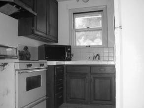
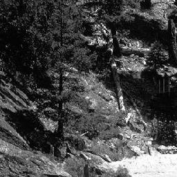
143 (a) kitchen living rm living rm living rm office (b) kitchen office (c) store mountain living rm inside city forest (d) industrial suburb (e) tall bldg inside city inside city mountain mountain mountain (f) tall bldg (g) inside city inside city suburb living rm living rm living rm suburb inside city open cntry tall bldg (h) street (i) highway store open cntry (j) coast coast open cntry Figure 6.4 Retrieval from the scene category database. The query images are on the far left, and the eight images giving the highest values of the spatial pyramid kernel (for L = 2, M = 200) are shown in decreasing order of kernel value from left to right. The actual classes of incorrectly retrieved images are listed below them. 134

144 6.4.2 Caltech101 Our second set of experiments is on the Caltech101 database [29], which was introduced in Section (Figure 3.13). As in Section 3.2.3, we follow the experimental setup of Grauman and Darrell [45], namely, we train on 30 images per class and test on the rest. For efficiency, we limit the number of test images to 50 per class. Note that, because some categories are very small, we may end up with just a single test image per class. Table 6.2 gives a breakdown of classification rates for different pyramid levels for weak features and strong features with M = 200. The results for M = 400 are not shown, because just as for the scene category database, they do not bring any significant improvement. For L = 0, strong features give 41.2%, which is slightly below the 43% reported by Grauman and Darrell. Our best result is 64.6%, achieved with strong features at L = 2. This exceeds the highest classification rate known to us so far, that of 53.9% achieved by our bag-of-features method in Section (Table 3.13) 3 Berg et al. [5] report 48% accuracy using 15 training images per class. Our average recognition rate with this setup is 56.4%. The behavior of weak features on this database is also noteworthy: for L = 0, they give a classification rate of 15.5%, which is consistent with a naive graylevel correlation baseline [5], but in conjunction with a four-level spatial pyramid, their performance rises to 54% on par with the best results achieved with much more discriminative local features by an orderless method. Figure 6.5 shows a few of the easiest and hardest object classes for our method. The successful classes are either dominated by rotation artifacts (like minaret), have very little clutter (like windsor chair), or represent coherent natural scenes (like joshua tree and okapi). The least successful classes are either textureless animals (like beaver and cougar), animals that camouflage well in their environment (like crocodile), or thin objects (like ant). Table 6.3 further illuminates the performance of our method by showing the top five of its confusions, all of which are between closely related classes. 3 This table lists the percentage of all test images classified correctly, which overestimates the per-class average, as discussed earlier. 135

145 Weak features Strong features (200) L Single-level Pyramid Single-level Pyramid ± ± ± ± ± ± ± ± ± ± ± ± ± ± 0.7 Table 6.2 Classification results for the Caltech101 database. minaret (97.6%) windsor chair (94.6%) joshua tree (87.9%) okapi (87.8%) cougar body (27.6%) beaver (27.5%) crocodile (25.0%) ant (25.0%) Figure 6.5 Caltech101 results. Top: some classes on which our method (L =2,M = 200) achieved high performance. Bottom: some classes on which our method performed poorly. class1/class2 class 1 misclassified class 2 misclassified as class 2 as class 1 ketch / schooner lotus / water lily crocodile / crocodile head crayfish / lobster flamingo / ibis Table 6.3 Top five confusions for our method (L =2,M = 200) on the Caltech101 database. 136

146 To summarize, our method has outperformed both state-of-the-art orderless methods [45, 168] and methods based on precise geometric correspondence [5]. Significantly, all these methods rely on sparse features (interest points or sparsely sampled edge points). However, because of the geometric stability and lack of clutter of Caltech101, dense features combined with global spatial relations seem to capture more discriminative information about the objects The Graz Dataset As seen from Sections and 6.4.2, our proposed approach does very well on global scene classification tasks, or on object recognition tasks in the absence of clutter with most of the objects assuming canonical poses. However, it was not designed to cope with heavy clutter and pose changes. It is interesting to see how well our algorithm can do by exploiting the global scene cues that still remain under these conditions. Accordingly, our final set of experiments is on the Graz dataset [118], which was introduced in Section (Figure 3.15). For this dataset, the range of scales and poses at which exemplars are presented is very diverse, e.g., a person image may show a pedestrian in the distance, a side view of a complete body, or just a closeup of a head. For this database, we perform two-class detection (object vs. background) using an experimental setup consistent with that of Opelt et al. [118]. Namely, we train detectors for persons and bikes on 100 positive and 100 negative images (of which 50 are drawn from the other object class and 50 from the background), and test on a similarly distributed set. We generate ROC curves by thresholding raw SVM output, and report the ROC equal error rate averaged over ten runs. Table 6.4 summarizes our results for strong features with M = 200. Note that the standard deviation is quite high because the images in the database vary greatly in their level of difficulty, so the performance for any single run is dependent on the composition of the training set (in particular, for L = 2, the performance for bikes ranges from 81% to 91%). 137

147 Class L = 0 L = 2 Opelt [118] Zhang Bikes 82.4 ± ± People 79.5 ± ± Table 6.4 Results of our method (M = 200) for the Graz database and comparison with two bag-of-features methods (refer back to Table 3.14). For this database, the improvement from L =0toL = 2 is relatively small. This makes intuitive sense: when a class is characterized by high geometric variability, it is difficult to find useful global features. Despite this disadvantage of our method, we still achieve results very close to those of Opelt et al. [118]. This is somewhat surprising, considering that their method uses a sparse, locally invariant feature representation, which is expected (at least in principle) to make it more robust to clutter and deformations. Note, however, that for this dataset, we cannot outperform our kernel-based orderless method of Section Discussion This chapter has presented a holistic approach for image categorization based on a modification of pyramid match kernels [45]. Our method, which works by repeatedly subdividing an image and computing histograms of image features over the resulting subregions, has shown promising results on three large-scale, diverse datasets. Note that in the experiments of this section, we validate the performance of the pyramid method by using several baseline tests: one baseline is obtained by omitting subdivision, resulting in a standard bag of features, and another one by using weak features instead of strong ones. Despite the simplicity of our method, and despite the fact that it works not by constructing explicit object models, but by using global cues as indirect evidence about the presence of an object, it consistently achieves an improvement over an orderless image representation. This is not a trivial accomplishment, since we have established in Chapter 3 that a well-designed 138

148 bag-of-features method can outperform more sophisticated approaches based on parts and geometric relations. Our results also underscore the surprising and ubiquitous power of global scene statistics: even in highly variable datasets, such as Graz, they can still provide useful discriminative information. It is important to develop methods that take full advantage of this information either as stand-alone scene categorizers, as context modules within larger object recognition systems, or as tools for evaluating biases present in newly collected datasets. 139

149 CHAPTER 7 Conclusion In the final chapter of this dissertation, we briefly recapitulate the main contributions of our research and discuss possible directions for future work. 7.1 Summary In this dissertation, we have considered a variety of image representations for recognizing textures, objects, and scenes. Our research has progressed from purely local models, which lack any geometric constraints save the coherence of the intensity pattern within each individual image patch, to semi-local models, which incorporate strong spatial constraints between relatively small groups of patches located close to one another, and finally, to global models, which record the absolute position of each feature within an image. In the following, we summarize the image representations considered in our work and highlight the most important experimental findings. Bag-of-features models. Chapter 3 has presented an orderless bag-of-features method for recognizing images of textured surfaces subject to large scale changes, rotations, perspective distortions, and non-rigid deformations. The use of local invariant features in this method has enabled us to handle a wider range of geometric variability than other existing texture analysis methods. This chapter has also presented extensive experiments on several texture and object datasets that have convincingly demonstrated the suitability of order- 140

150 less methods for classification of object images, despite substantial noise in local feature distributions introduced by clutter and uncorrelated backgrounds. Because this method is conceptually primitive, yet surprisingly effective on real-world data, we view it as a good baseline against which to evaluate alternative methods that incorporate more sophisticated spatial constraints. Neighorhood co-occurrence relations. Chapter 4 has considered methods for extending the purely local bag-of-features model with statistical co-occurrence relations between pairs of nearby features. The resulting image representation is a conceptual analogue of a bigram model for natural language. In the experiments of this chapter, relations did not improve the accuracy of whole-image classification, but they did prove useful for the more challenging task of labeling individual features in multi-texture images. Semi-local parts. Chapter 5 has introduced a structured object representation based on multiple composite geometrically stable parts. This method has more descriptive power for modeling objects than orderless bags of features, and it achieves higher classification rates on our bird and butterfly databases. Moreover, because our approach relies on explicit geometric alignment search, it is capable of higher degrees of invariance than probabilistic constellation models, and can find larger object models in substantial clutter. Spatial pyramid matching. Chapter 6 has presented a global method for recognizing scene categories that works by establishing approximate geometric correspondence between sets of local features found in two images. This method is simple and efficient, and shows much higher performance than the bag-of-features baseline on one scene and two object datasets. Even though this approach is not geometrically invariant, it makes effective use of multiple training exemplars to learn intra-class appearance variations. Overall, each of the models considered in this dissertation has demonstrated its usefulness on a particular class of recognition problems. At this stage, however, we still have a fairly incomplete understanding of models that combine local features or parts with co-occurrence 141

151 relations. As shown by our experiments with the discriminative maximum entropy framework (Section and Section 5.3.2), co-occurrence relations for textons and overlap relations for parts did not improve the performance of whole-image classification of textures and objects, respectively. However, co-occurrence relations did prove useful for labeling individual regions in multi-texture images (Section 4.2.2), and we conjecture that inter-part relations will likewise prove useful for object localization. Intuitively, the more demanding the recognition task (i.e., the more detailed the explanation of the image that must be supplied by the recognition algorithm), the more elaborate the image representation should be. In most experiments, we have considered exclusively whole-image classification, which is the simplest task, since it requires a single label for the entire image. In the future, we plan to devote more attention to more complex image interpretation tasks, which should yield additional insights into the role of spatial relations in image models. 7.2 Extensions In the future, we will work towards improving the flexibility, discriminative power, and expressiveness of our image models to make them applicable to a wider range of challenging imagery, including objects that lack characteristic texture, and those that are highly nonrigid and articulated (Figure 7.1). Figure 7.1 Images that challenge the capabilities of our current representation methods: Objects that lack texture, such as the plaster head and the glass vase, do not lend themselves to a patch-based representation. The spots and colors of the cows are not characteristic of their class, and neither is the clothing that people wear. Human bodies are highly articulated and their limb structure may not be clearly visible in a photograph. 142