LEARNING MODELS FOR MULTI-VIEWPOINT OBJECT DETECTION

Transcription

1 LEARNING MODELS FOR MULTI-VIEWPOINT OBJECT DETECTION Akash M. Kushal, Ph.D. Department of Computer Science University of Illinois at Urbana-Champaign, 2008 Jean Ponce, Adviser This dissertation addresses the task of detecting instances of object categories in photographs. We propose modeling an object category as a collection of object parts linked together in a deformable configuration. We propose two different approaches to model the appearance of object parts that provide robustness to intra-class variations and viewpoint change. The first approach models object parts as locally rigid assemblies of dense feature points and part detection proceeds by incrementally matching the feature points between the model image and the test image. The second approach employs a discriminative classifier (Support Vector Machine) based on a descriptor that consists of a combination of a sparse visual word histogram pyramid and a dense gradient and edge histogram pyramid. We also propose two different approaches for modeling the inter-part relations and algorithms for efficiently learning the model parameters. The first approach uses a generative model that models the joint probability distribution over the locations and visibility of all the object parts. The second approach employs a discriminative Conditional Random Field based model to encode the relative geometry and co-occurrence constraints.

2 c 2008 Akash M. Kushal

3 LEARNING MODELS FOR MULTI-VIEWPOINT OBJECT DETECTION BY AKASH M. KUSHAL B.Tech., Indian Institute of Technology, 2003 M.S., University of Illinois at Urbana-Champaign, 2005 DISSERTATION Submitted in partial fulfillment of the requirements for the degree of Doctor of Philosophy in Computer Science in the Graduate College of the University of Illinois at Urbana-Champaign, 2008 Urbana, Illinois Doctoral Committee: Professor Jean Ponce, Chair Professor David A. Forsyth Professor Thomas S. Huang Professor Dan Roth Dr. Cordelia Schmid, INRIA

4 Abstract This dissertation addresses the task of detecting instances of object categories in photographs. We propose modeling an object category as a collection of object parts linked together in a deformable configuration. We propose two different approaches to model the appearance of object parts that provide robustness to intra-class variations and viewpoint change. The first approach models object parts as locally rigid assemblies of dense feature points and part detection proceeds by incrementally matching the feature points between the model image and the test image. The second approach employs a discriminative classifier (Support Vector Machine) based on a descriptor that consists of a combination of a sparse visual word histogram pyramid and a dense gradient and edge histogram pyramid. We also propose two different approaches for modeling the inter-part relations and algorithms for efficiently learning the model parameters. The first approach uses a generative model that models the joint probability distribution over the locations and visibility of all the object parts. The second approach employs a discriminative Conditional Random Field based model to encode the relative geometry and co-occurrence constraints. ii

5 To my mom and dad iii

6 Acknowledgments I would like to thank my adviser, Prof. Jean Ponce, for his invaluable guidance. He has taught me a great deal about shaping and presenting research. I would also like to thank the members of my committee, whose different perspectives greatly enhanced my research experience. I would like to thank my lab-mates over the years - Fred Rothganger, Kenton McHenry, Yasutaka Furukawa, Lana Lazebnik, Sourabh Bhattacharya, James Davidson, Sal Candido, Himanshu Arora, Avinash Kumar and Julien Mairal - with whom I have had an invaluable exchange of ideas and inspiration throughout our time as graduate students. I would like to thank Fred Rothganger for providing the FL library which has been used as a base for most of my code. I would also like to thank Lana Lazebnik for her circle detection code. Finally, I would like to especially thank Kenton McHenry for his tireless efforts to maintain our lab s infrastructure. I would like to thank my family, who has always supported me in all my endeavors. I would also like to thank my friend Soumyadeb Mitra for helping me with all sorts of problems (technical and otherwise) and for keeping me motivated throughout these years. This work was supported in part by the National Science Foundation under grant IIS , the UIUC/INRIA/CNRS collaboration agreement, and the INRIA associated team Thetys. iv

7 Table of Contents Chapter 1 Introduction Object Recognition Task Image Classification Object Detection Part Models Contributions and Outline Chapter 2 Background Feature Detection Feature Descriptors Object Models Bag-of-Part Models Geometrically Rigid Part Models Locally Orderless Models True Multi-Viewpoint Models Chapter 3 A Generative Multi-View Model for Object Detection Partial Surface Models Representing Parallelograms as Affine Transformations Viewpoint Annotation Base Image Matching PSM Initialization PSM Hypothesis Expansion PSM to Image Matching PSM Match Representation Geometric Filtering PSM Validation and Selection PSM Appearance Model Training Data Construction Training the Classifier The PSM Graph Generative Model for PSM Detections Object Model Background Model v

8 3.5 Learning Model Parameters Constructing the Training Data Parameter Learning Object Detection and Localization Detection Localization Experiments and Discussion Evaluation Method PSM Voting and Mean Shift Results Chapter 4 A Discriminative Geometric Model for Multi-View Object Detection Introduction Discriminative Object Model Association Potential Interaction Potential Model Learning Gradient Approximation for Learning Loopy Belief Propagation on the CRF Object Detection Results and Discussion Chapter 5 A Discriminative Appearance Model Introduction Motivation Discriminative Part Models Data Preprocessing DPM Initialization DPM Appearance Description SVM Learning Efficient Computation over Scanning Windows Geometric Model Association Potential Interaction Potential Parameter Learning Gradient Approximation for Learning Object Detection Experimental Results Chapter 6 Conclusions and Future Directions Contributions Future Directions Appendix A Non-linear Match Refinement vi

9 Appendix B Logistic Regression and Conditional Random Fields as Maximum Entropy Models Appendix C Learning Geometric Parameters for the PSM Graph C.1 Approximate Loopy Belief Propagation on the PSM Graph C.2 Optimizing the Parameters References Author s Biography vii

10 Chapter 1 Introduction Object recognition or, in a broader sense, scene understanding is the ultimate scientific challenge of computer vision: After 40 years of research, robustly identifying familiar objects (chair, person, pet), scene categories (beach, forest, office), and activity patterns (conversation, dance, picnic) depicted in family pictures, news segments, or feature films is still far beyond the capabilities of today s vision systems. On the other hand, truly successful object recognition and scene understanding technology will have a broad impact in application domains as varied as defense, entertainment, health care, human-computer interaction, image retrieval and data mining, industrial and personal robotics, manufacturing, scientific image analysis, surveillance and security, and transportation. The object category recognition problem is complicated by various factors such as intraclass variations in appearance and geometry between different object instances (figure 1.1), variations in lighting conditions (figure 1.2) and variations in camera viewpoint (figure 1.3). Despite the limitations of today s scene understanding technology, tremendous progress has been accomplished in the past five years, due in part to the formulation of object recognition as a statistical pattern matching problem. The emphasis is in general on the features defining the patterns and the machine learning techniques used to learn and recognize them, rather than on the representation of object, scene, and activity categories, or the integrated interpretation of the various scene elements. Modern pattern-matching approaches typically focus on fronto-parallel views of mostly upright, nearly rigid objects, such as faces and mo- 1

11 Figure 1.1: Intra-Class Variation Figure 1.2: Lighting Variation Figure 1.3: Viewpoint Variation torbikes, and they have proven successful in that domain for images with moderate amounts of clutter and occlusion. In this thesis we propose to develop models for truly 3D object category recognition that employ discriminative parts and inter-part relations that are robust to many of the sources of variablity described above. 2

12 1.1 Object Recognition Task The object recognition task can be thought of in at least two different ways. Scene understanding goes beyond image classification and object detection, and is concerned with the analysis of the relationships among scene components, an even harder problem beyond the scope of this dissertation Image Classification Object recognition may be considered as an image classification problem where we seek to label each image with the category labels for the object instances present in the image. For such tasks, orderless bag-of-feature methods [16, 42, 43, 99, 101] have been shown to perform well. A brief description of this type of approach is provided in section Such local feature-based approaches have also been used for texture classification [53], video retrieval [89] and scene classification [22, 64]. Even though these approaches perform well for classifying images based on the presence or absence of the object it is hard to adapt them to separate the object from the background. This is partly because of the fact that the foreground and background features are usually correlated and these methods cannot distinguish between them Object Detection In this thesis, we are concerned with the harder problem of detecting the instances of a given object category as well as localizing them in a target image. The methods for the detection task typically model some level of spatial consistency between different object parts. Scanning window based approaches [13, 17] move a window at multiple scales in the image and classify the window region based on a spatial histogram of image features extracted from the region. Other approaches [3,25,26,58,61,97] as well as those described in this thesis model object parts and inter-part relations explicitly. 3

13 1.2 Part Models In these models, the objects are modeled as collections of object parts with or without geometric and/or co-occurance constraints among the parts. The parts are usually associated with appearance models that are used to detect possible part instances at multiple image locations. The inter-part constraints are then used to combine the part detections together into object instances while at the same time pruning false part detections. The models proposed in this thesis impose specially designed local geometric constraints which make them robust to viewpoint variations. Using a part based approach as opposed to classifying the entire object region simultaneously has the following advantages. Robustness to occlusion: Since object parts are relatively small one can expect some of them to be visible even when others have been occluded. If enough of these parts are detected, they may provide sufficient evidence to be able to detect the object even when parts of it are occluded. Modeling of deformations: Again, due to their relatively small extent, the change in appearance caused by non-rigid deformations or viewpoint change can be modeled more reliably for object parts. This provides higher repeatability in detection of object parts. Modeling of appearance: The amount of variability in appearance of a part is significantly smaller than than the appearance variation for the entire object. If we consider an object with P parts where each part takes on one of K appearances independently of others, we get a total of K P different appearances for the object. Due to this exponential increase, modeling the variability for the parts independently and then combining the detections later is a more feasible approach. In practice, the appearances of the different objects parts are not independent and one may wish to model these inter-part correlations after the initial part detection stage. 4

14 1.3 Contributions and Outline In this thesis, we propose two approaches for modeling the appearance of object parts. The first approach models object parts as Partial Surface Models (or PSMs) which are collections of local image features linked together in a locally affine rigid structure (see [52, 53] for a related approach using a globally affine rigid structure). Enforcing the geometric relations only locally among neighboring features allows the PSMs to be highly discriminative while at the same time being flexible enough to allow significant viewpoint change. The PSMs employ a combination of salient image regions as well as a grid of texture patches in the model image to achieve a dense coverage of the object part area. We provide algorithms for automatically learning the PSMs from a set of training images containing the object category as well as for detecting the learned PSMs in test images containing the object. The second approach models an object part using a support vector machine constructed on a feature vector consisting of a dense gradient and edge histogram-based descriptor and a sparse visual words histogram-based descriptor. Again we provide algorithms for learning these discriminative classifiers which we call Discriminative Part Models (or DPMs) automatically from training images containing the object instances. We also propose two different techniques for modeling the inter-part relations. The first approach models the joint probability distribution over the visibility and affine positions of all the object parts using a probabilistic graphical model (dubbed the PSM-Graph). Links are constructed between nearby object parts and encode the relative geometric relationships between them in a way that is robust to viewpoint changes. We also describe algorithms to automatically learn the link parameters from parts detected in the training images. 5

15 The second approach employs a discriminative conditional random field (CRF) [50] to model the co-occurrence and geometric relations between the object parts. The geometric potentials are specially designed to model the relative geometry of two parts on a single smooth surface or on two intersecting smooth surfaces. The potentials also allow modeling of the geometric relationship between two parts that are rigidly attached at a single point but may deform with respect to each other. Again we provide efficient algorithms for automatically learning the inter-part relations from training images. The rest of this dissertation is organized as follows. Chapter 2 provides a short review of the vast existing literature on object recognition. In chapter 3, we describe an approach that employs partial surface models (or PSMs) to represent object parts and the PSM-Graph (mentioned above) to model the inter-part relations. The discriminative CRF based interpart model is described in chapter 4. Chapter 5 that combines this CRF based inter-part geometric model with the SVM based discriminative part models (or DPMs) mentioned above to model the part appearances. Finally, chapter 6 provides conclusions and some future directions for research. Throughout this thesis, the proposed object recognition methods are evaluated on standard datasets such as the PASCAL VOC Challenge 2005 and the PASCAL VOC Challenge 2007 datasets. The approaches are shown to achieve state-of-the-art performance on these challenging datasets. 6

16 Chapter 2 Background In this chapter we provide a brief survey of the prior work in object recognition and motivate the approaches presented in the thesis. Since all of the approaches described in this thesis use feature detection and matching at some stage, we begin with a brief overview of the literature on this topic. 2.1 Feature Detection The feature detection process aims to select salient patches that capture much of the discriminative information in an image. Looking at an image as a set of features allows us to transform the continuous object detection or image matching problem into a discrete feature matching problem. The features considered in this work are small parallelogram shaped image regions. The feature extraction process involves an initial feature detection step followed by a scaling and normalization step which allows the extracted feature to be invariant to a variety of geometric transformations. This process adapts the shape of the detected feature based on the image texture around it to determine a canonical shape for the feature. The key reason for this adaptation process is to make the appearance of the detected and normalized features invariant to geometric deformations due to scale and viewpoint variations. The Harris detector [34] is a popular scheme for detecting corner features in images. 7

17 Lindeberg [60] describe a blob detector based on maximum of the Laplacian. The scale is automatically selected to be the one where a normalized Laplacian achieves its maximum. A similar detector is the Hessian detector [70, 71] which is based on the determinant of the Hessian matrix and gives strong responses on blobs and ridge-like features. This detector also employs an affine adaptation process based on the second moment matrix developed by Garding and Lindeberg [32]. This process determines the affine shape of the detected feature upto a rotation. The rotation may be determined by normalization based on the dominant gradient orientation [63, 70]. Affine covariant versions of the Harris detector are described in [70, 71, 88]. Jurie et al. describe an edge based salient region detector in [41]. The detector selects circular regions for which the detected contour strength along the tangential orientation of the circle is large and the contour occurs for a wide range of orientations around the circle. The regions detected are invariant to scale and rotation - though a normalization process based on the dominant gradient orientation is required before descriptor computation to achieve rotation invariance. A comparative evaluation of recent state-of-the-art salient feature detectors is presented in [72]. One may choose to use scale-invariant, scale and rotation invariant, or fully affine invariant detectors based on the kind of geometric transformations one expects to encounter in a given problem. If the datasets contain images where the viewpoints are unconstrained, choosing a low level of invariance would require modeling the appearance of the same object feature from different viewpoints using different model features. Hence, it would be beneficial to use a fully affine-invariant feature detection scheme and model the features normalized appearance once. However, since some of the discriminating texture information is normalized away during the feature adaptation process, a higher level of geometric invariance comes at the cost of decreasing the discriminative capacity of the resulting normalized texture patch. Hence, if the images one expects to deal with contain the object only under a restricted class of geometric transformations it is usually better to choose the corresponding 8

18 Figure 2.1: Left column : Top 100 circle detections for the images - using the implementation of Lazebnik et al. [53] of the circle detector described in Jurie et al. [41]. Right column : Top 100 Hessian-Laplace feature detections - using the implementation of Mikolajczyk et al. [71]. level of geometric invariance during feature detection. In this thesis, we deal with objects observed from varying viewpoints however the camera axis usually remains horizontal. Hence, we choose scale invariant detectors for the methods described. This restricts the amount of deformation we may model due to change of viewpoint (mainly a rotation about the vertical) and hence we employ a match refinement procedure (described in appendix A) to provide a limited amount of robustness to this viewpoint variation. 9

19 Figure 2.2: Histogram based descriptors - the SIFT descriptor [63] (left), GLOH descriptor [74] (center) and the shape context descriptor [6] (right). 2.2 Feature Descriptors After detecting features we are now faced with the problem of matching them between the model and the target images. Feature descriptors allow us to characterize the appearance of the image texture around the appropriately normalized features to facilitate their matching. A good descriptor must be robust to intra-class variations in appearance as well as to lighting variations while at the same time retain the key texture information in the feature and provide strong appearance based cues while matching. A classic approach towards feature description is to use a set of linear filters such as Gabor filters [30, 66], wavelets [96] or steerable filters [29]. More recently, histogram based descriptors such as the Scale Invariant Feature Transform (or SIFT) [63], the Gradient Location and Orientation Histogram (or GLOH) [74] and Shape Context [6] have become popular and have been shown to perform well in image and shape matching tasks. These descriptors work by placing a grid on the normalized feature and accumulating edge or gradient intensities along a set of orientations at all the locations within the cells of the grid. Considering gradients and edges provides robustness to lighting conditions and the histogramming provides robustness to small alignment errors and small intraclass variations in the appearance of the feature. The SIFT descriptor uses a rectangular 4 4 grid of histogram bins and 8 angular orientations to construct a 128 dimensional vector describing every feature. On the other 10

20 Figure 2.3: SIFT descriptor [63] - the image patch (left) and the corresponding SIFT descriptor (right). hand, both the GLOH and shape context descriptors use a log polar grid in a circular region around the feature where the radial sizes of the bins become larger as they move farther from the center of feature. The GLOH descriptor accumulates the gradients along a set of 16 orientations for each of 17 spatial bins whereas the shape context descriptor accumulates only the edge counts in each of its 60 spatial bins (5 radial bins in each of the 12 angular sectors) and ignores their orientation (see figure 2.2). Ke et al. [44] propose reducing the dimensionality of the histogram based descriptors (like SIFT) using Principal Component Analysis (PCA) to create a lower dimensional descriptor called PCA-SIFT. Mikolajczyk et al. [74] use this idea and reduce the dimensionality of the GLOH descriptor from the original to 128 (to equal the SIFT descriptor). A comparison of the performance of feature descriptors is provided in [74]. The authors conclude that SIFT and its derivatives (such as GLOH) achieve the best performance. 11

21 2.3 Object Models This sections reviews some popular object models employed in recognition approaches. We categorize the models into the following categories Bag-of-Part Models Bag-of-parts approaches model the object as a collection of object parts without any geometric relations between them. These approaches are motivated by the bag-of-words paradigm for text classification [10,35,69,77,86]. The object parts may be simple features [16,54,99,101] (in which case the method could be called a bag-of-features method) or more complicated parts which consist of multiple features (as in [53]). In a simple bag-of-features approach [16, 99, 101], a vocabulary of visual words is constructed by clustering a large collection of image features across all images. The local features extracted from the image are quantized using this vocabulary and the distribution of the visual words is captured using a histogram which defines a feature vector describing the image. A discriminative classifier is then used to distinguish between the images that contain instances of an object class and those that do not. Lazebnik et al. [53] propose using a more discriminative part model. They represent object parts as a collection of multiple features linked together in an affinely rigid structure. More precisely, each feature point s location and shape is fixed rigidly within the object part but the entire part and all the features within it may deform together using a single common affine transformation. Lazebnik et al. [53] also provide a hypothesize-and-validate framework to automatically learn the object parts from multiple images containing the object. Using multiple features together increases the discrimination ability of the part and allowing the part to affinely deform as a whole provides a limited amount of robustness to viewpoint change and intraclass variations. However, significant viewpoint change results in the affine rigidity assumption to break down and part detection to fail. Each part is detected by 12

22 matching the features in the part to the features detected in the target image. The number of features matched for every part is used as an estimate for the quality of the part detection. The quality scores for each object part are combined to form a feature vector for the target image which is then classified using a maximum entropy classifier [83] to detect the presence of the object in the target image. Grauman et al. [42] propose an efficient method to quickly compute a matching score between two sets of features by approximating the bijective point to point matching score using the pyramid-match kernel [42]. The authors employ this kernel in a support vector machine framework for object categorization by using the features detected in the images directly instead of first quantizing them into visual words. One of the approaches described in this thesis (chapter 3) extends the part model proposed by Lazebnik et al. [53] and represents object parts as dense, locally rigid assemblies of texture patches to gain additional robustness to viewpoint change and intra-class variations in part appearance. We augment the primary interest point features of [53] with more general secondary texture patches to generate dense object parts and use all the texture information available available for the part. Using dense as opposed to sparse models has also been shown to be beneficial for the single object recognition problem 1 [27,28,48]. The local rigidity allows the parts to have additional robustness to viewpoint variation and geometric deformation caused due to intraclass variations. The advantage of the bag-of-parts approach is that they can be used to construct multiviewpoint object models since it does not enforce any geometric constraints. This is also a disadvantage since these geometric constraints can often be very useful in pruning misdetections. 1 The single object recognition problem is concerned with recognizing a specific object instance as opposed to an object category. This is a considerably simpler problem since it does not involve modeling the intra-class appearance and geometric variations that need to be modeled for object categories. 13

23 (a) Bag of parts - Zhang et al. [101], Lazebnik et al. [53], Csurka et al. [16] LandmarkP art (b) Constellation model - Fergus et al. [25] Object center and scale (c) Star model - Fergus et al. [26] (d) Star model of Arora et al. [3] and Loeff et al. [61] (e) Histogram based descriptor of Dalal et al. [17], Chum et al. [13] (f) Models proposed in this thesis connect parts across different viewpoints. The dotted lines depict that the geometric constraints used are robust to viewpoint change Figure 2.4: The geometric constraints imposed by various models. 14

24 2.3.2 Geometrically Rigid Part Models Weber et al. [97] and Fergus et al. [25] propose a constellation model where the object is modeled as a collection of parts and the relative geometry of the parts is modeled using a generative model. Fergus et al. represent object parts using simple interest point features and model the joint probability distribution over the part locations as a Gaussian distribution with a full covariance matrix. Once the global scale of the object is fixed, each part s location is modeled using its x, y image coordinates which makes the model highly viewpoint specific. This is because the relative x, y coordinates of the object parts are not conserved under viewpoint change. In addition, the learning time is exponential in the number of parts, which limits the number of parts in the model to a maximum of 6 or 7. Fergus et al. propose in [26], a star model where they specially designate one of the object parts to be a landmark part. The geometric locations of the model parts relative to this landmark part are assumed to be generated from independent Gaussian distributions. This assumption significantly reduces the complexity of model learning and inference however the geometric constraints used are still rigid and hence valid only for a single viewing direction. Loeff et al. [61] and Arora et al. [3] also propose star models however they do away with the requirement of using a landmark part. They propose a generative model for the object where the object generates a number of parts, each of which generates features with a certain appearance and location relative to the object center. The appearance of the features is modeled as a multinomial distribution over a codebook of feature types and the relative location is modeled as a Gaussian with a mean and covariance for each part. The appearance model of a single part is rather weak in this case since all the features for a given part are generated with independent locations relative to the part center. In addition, the star model enforces rigid geometric constraints among the different object parts and so becomes viewpoint dependent. Crandall et al. [15] specially designate a set of k central parts and assume that the geometric locations of all the other parts are independent given these 15

25 k central parts. Their k-fan model provides an intermediate level of geometric consistency modeling between the constellation model and the star model. Another approach in the same category is the implicit shape model (or ISM) of Leibe et al. [58]. Leibe et al. cluster the feature points detected on the object into a set of visual words and store, for each visual word, the location of the object center and scale relative to the visual word. During recognition, each feature detected on the test image essentially casts probabilistic votes for object centers and scales and a mean shift procedure is used to find the maxima in this space. Again since the position of each feature relative to the object center is fixed given the global object scale, the geometric constraints are viewpoint dependent and the model is thus valid only for a single aspect of the object Locally Orderless Models Dalal et al. [17] scan the entire image at multiple positions and scales with a detection window characterized by a histogram of oriented gradients (HOG). Each detection window is then classified as object/background by using a linear SVM over the corresponding HOG feature vector. The HOG feature vector is similar in spirit to the SIFT descriptor [63] and is computed by placing a rectangular grid on the detection window and accumulating gradients along a set of orientations within the rectangular bins. However, the HOG feature employs a local (as opposed to a global) normalization step and the number of bins in the HOG grid are carefully engineered to achieve very good detection performance [19]. Lazebnik et al. [55] propose a pyramid based descriptor for scene classification where muliple spatial bins in a lower layer are merged together in the layer above. Chum et al. [13] propose a similar scanning window based detector that uses a combination of a dense histogram of edge orientations and a sparse histogram of visual words where the histograms are constructed in a pyramid setup (similar to [55]). Chum et al. employ an SVM with a chi-squared kernel for classification of the scanning window. Note that both the HOG descriptor [17] and the descriptor of Chum et al. [13] enforce rigid geometric constraints between the different 16

26 object regions and are hence single aspect models. Chum et al. independently construct one such model for each of a set of different viewpoints around the object to construct a multi-viewpoint detection system which achieves achieves good detection performance on challenging datasets such as the PASCAL VOC 2007 Challenge [20]. One of the methods described in this thesis (chapter 5) uses a feature vector very similar to that of Chum et al. to represent individual object parts. Felzenszwalb et al. [24] train a single linear SVM detector based on the HOG descriptor of Dalal et al. [17] but augment the detector for the entire object with smaller part detectors. The parts are allowed to shift around within a small search area around their fixed mean positions within the detected object. Adding this additional part layer to their model allows them to improve performance over the simple HOG based detection scheme of [17] True Multi-Viewpoint Models In this section, we review some of the recognition approaches that use a common object model across different viewpoints instead of modeling each aspect of the object independently. The advantage of such models is that there is an infinitely large space of possible viewpoints and it is hard to densely sample all possible viewpoints one may observe. Also, constructing just one model for a given object part s appearance across the different aspects and modeling the change of appearance due to viewpoint change explicitly allows using the entire training data where the part is visible to construct the appearance model of the part. The training data is thus used much more efficiently while learning such a model. We begin by describing some multi-viewpoint approaches proposed in the single object recognition domain. Huttenlocher and Ullman [37] describe an algorithm for detecting polyhedral objects represented using wireframe models in images. They compute the matching score based on the consistency of the actual edges detected in the image and the those predicted by projecting the object into the image using an orthographic projection. Rothganger et al. [84] have proposed learning a 3D patch based representation of the target object from 17

27 multiple un-calibrated training images of the object. The patches in the model correspond to features detected and matched across the training images using wide-baseline stereo techniques [5, 68, 81, 90, 93] and their 3D positions are determined using structure from motion techniques [80, 92, 98]. Once the 3D object model has been learned, the object detection proceeds by matching the features between and the model and the test image and using the 3D geometric structure of the object to provide tight and accurate constraints to guide the feature matching process and pruning false matches. Kushal et al. [48] also build a patch based 3D model but they augment the primary interest point patches used by Rothganger et al. [84] with more general secondary texture patches to construct a dense 3D representation of the object. These dense models are constructed using an expansion technique [28] where already matched features are used to predict matches for nearby unmatched texture patches. The partial surface models described in chapter 3 employ a similar expansion technique to create a dense appearance model for the object parts. Ferrari et al. [27] integrate the information contained in images with neighboring viewpoints by constructing region tracks consisting of the same region of the object seen in multiple views. They introduce the notion of a group of aggregated matches (GAM) which is a collection of matched regions on the same surface of the object. The region tracks are then used to transfer matched GAMs from one model view to another, and their consistency is checked using a loose heuristic test. In the object category recognition domain, Thomas et al. [91] have proposed a technique which deals with the viewpoint change problem by combining models learned for different viewpoints. They use a highly supervised dataset that consists of images of multiple motorbike instances, each from a set of up to 16 viewpoints. First, they construct separate viewpoint dependent ISMs [58] for each of the different viewing directions. Then, they use the method of Ferrari et al. [27] to match the images of the same motorbike instance across different viewpoints and construct region tracks that are later used to transfer the ISM votes from one viewpoint to its neighboring viewpoints. This is an interesting setup, but it re- 18

28 quires highly supervised training data and a dense sampling of viewpoints since the ISMs themselves are highly viewpoint dependent. In addition, since each of the ISMs is learned independently, there is no sharing of parts among the different viewpoints. In contrast, the methods described in this thesis employ a single appearance model for object parts across different viewpoints. 19

29 Chapter 3 A Generative Multi-View Model for Object Detection In this chapter, we describe a multi-viewpoint object model that relies on the observation that even though the geometric relationship between distant parts of an object may vary due to intra-class variability and changes in viewpoint, the relative geometry of close by parts is much more robust to these factors. In particular, the relative affine transformations among nearby parts on a smooth surface can be shown to be robust to viewpoint change. This is related to the well known fact that arbitrary smooth deformations including those induced by viewpoint change for affine cameras or perspectives ones far from the scene relative to its relief are locally equivalent to affine transformations [45]. Here, we represent object parts as partial surface models (or PSMs) which are dense, locally rigid assemblies of image patches. These PSMs are learned by matching repeating patterns of features across training images of each object class (Section 3.1). Pairs of PSMs which regularly occur near each other at consistent relative positions are linked by edges whose labels reflect the local geometric relationships between these PSMs. These local connections are used to construct a probabilistic graphical model for the geometry and appearance of the PSMs making up an object (Section 3.3). The corresponding PSM graph is the basis for an effective algorithm for object detection and localization (Section 3.6), which outperforms the state-of-the-art methods compared in [19] on the Pascal 2005 VOC 20

30 Challenge Cars Test 1 data (Section 3.7). 3.1 Partial Surface Models We extend the sparse and affinely rigid parts of Lazebnik et al. [52,53] to make them more robust to intra-class variations and viewpoint change. We term these part models partial surface models or PSMs. Like the parts used by Lazebnik et al. [52,53], PSMs are also formed by linking together multiple feature points in a geometric configuration. Using multiple linked features instead of a single feature point to describe the part appearance makes the parts more discriminative and provides some added robustness to occlusion and intraclass variations. The two key differences between the PSMs proposed in this thesis and the parts proposed by Lazebnik et al. [52,53] are the following. Dense feature representation: Lazebnik et al. [52, 53] use only interest point features to construct their object parts. Dense patch based representations which employ general texture patches instead of only interest point based patches have been shown to be beneficial for image matching and object detection tasks [27,28,48,49]. The extra texture information makes the appearance model more discriminative and also helps to add continuity to the part matching process (section 3.1.5) for more reliable matching. We call the standard interest point feature points as primary patches and the extra texture patches generated in a grid all over the image as secondary patches. The key distinction between the two types of patches is that only the primary patches are repeatable and can be matched directly between images. The secondary patches are not repeatable in general and must be matched by using an expansion procedure (described in section 3.1.5) which uses nearby patches that have already been matched to predict matching locations for the secondary patches. Local affine rigidity assumption: The features within the PSM are linked by local affine rigidity constraints. More precisely, only features that are in the vicinity of each 21

31 S (1, 0) (0, 0) (0, 1) u p v rectified patch (canonical frame) image parallelogram Figure 3.1: Representing the red parallelogram in the image (right) with the 6 degree of freedom affine transformation S. S maps the blue canonical square at the origin with sidelength 2 (left) to the target parallelogram. other are directly constrained to deform using a similar affine transformation while matching. This gives the PSMs more flexibility as compared to the parts of [52,53] which require all the features to deform using the same global affine transformation Representing Parallelograms as Affine Transformations Before describing the PSM learning process in detail we first describe a notation we will use throughout this thesis for representing parallelograms in images. We can parameterize any parallelogram in the image using the following three quantities which correspond to the 6 22

32 degrees of freedom of the parallelogram - its center of mass p and the 2 vectors u and v from the center of mass, running parallel to the two edges of the parallelogram and ending at the boundary of the parallelogram (see figure 3.1). Let us consider the canonical square centered at the origin, with sides parallel to the x and y axes and having a side length of 2. It is easy to verify that affine transformation that maps this square into the target parallelogram with parameters p, u and v is S = u v p Throughout the thesis we will use this 6 degree of freedom transformation to represent parallelogram shaped regions in the image. This representation (after [84]) allows us to succinctly represent the relative geometric relations between different parallelograms in the same image Viewpoint Annotation Since the object category we are concerned with in the experiments described at the end of this chapter (cars) is symmetric (i.e. images of cars facing left are identical, up to a flip about the vertical, to those of cars facing right), we learn a model to detect only cars facing right. The detector is run on the original images as well as their flipped versions to be able to detect cars facing both to the left and to the right. To make full use of the training data while learning the object model, we correct each image of the training set so that the car is pointing towards the right (by flipping the image, if required). We also annotate the images with a rough viewing direction from the set {Rear, RearSide, Side, SideF ront, F ront}. Some of these viewpoint annotations (those for Rear, Side and F ront) are already available in the training data we use - the PASCAL VOC 2005 Challenge dataset. We now describe the process of learning the PSMs automatically from training images containing instances of the object with their bounding boxes labeled. 23

33 3.1.3 Base Image Matching The PSMs are learned using a hypothesize-and-validate framework (similar to Lazebnik [52,53]). The learning process starts by selecting two images at random from the training set and computing appearance-based primary matches between pairs of salient regions detected in the images. The two images selected are called the base images for the PSM. We will refer to them as I 1 and I 2. To avoid an excessive reliance on characteristic feature patterns, we use a circle detector (proposed by [41]) to detect the salient image regions. We use the implementation of Lazebnik et al. [53] which employs a Hough transform step followed by non-maxima suppression to efficiently detect the circles in edge maps computed at different scales in a scale pyramid constructed on the image. We output the smallest axis parallel square containing the detected circles as salient regions. These regions are then described by using the SIFT descriptor of David Lowe [63] and candidate matches are computed between the detected feature points in the two training images. The matches which have a correlation greater than a threshold T l = 0.6 are considered valid. While computing the matches, we ignore all the interest points detected outside the bounding box of the object instance to reduce the amount of false matches generated. Next, a non-linear match refinement process (described in detail in Appendix A) is used to correct the initial alignment of these matches. The original square shaped patch in one of the two base images is kept fixed and the other patch is allowed to deform into a parallelogram using a 6 degree of freedom affine transformation. The refinement process optimizes this affine deformation to maximize the correlation between the SIFT descriptors of the two matched patches. Figure 3.2 shows an example of this refinement process. Since we use the scale invariant circle detector of [41] the refinement process is essential to make the matching process robust to viewpoint change. A threshold on the SIFT correlation score after refinement T h = 0.65 is used to prune the appearance matches further to get the set of candidate matches for the next stage. Figure 3.3 shows the base image matching process 24

34 Refinement Image I 1 Image I 2 canonical frame Figure 3.2: The match refinement process. The top row shows the matched patches in the two images and their rectified versions in their canonical coordinate frame. The second row shows the patches and rectified versions after the refinement process. The patch in the second image is deformed to improve its alignment with the first image patch. for two example images PSM Initialization Once candidate matches have been found, they are partitioned into locally consistent PSM hypotheses using a greedy approach. Each PSM hypothesis is initialized with a single match. Then, nearby matches are iteratively added to the PSM hypothesis as long as they are locally consistent with the matches already included in the PSM. Next, we formally define what we mean by nearby and locally consistent in the above statement. We define the asymmetric dissimilarity d(s 1, S 2 ) of patch S 1 from patch S 2 in the same image as follows. We first compute the pre-image of the patch S 1 into the canonical frame of S 2 as S 12 = S 1 2 S 1. If S 1 and S 2 are close to each other we would expect the transform S 12 to be close to the identity matrix I 3 3. We define the dissimilarity as 25

35 selected base images interest point matching match refinement Figure 3.3: Base image matching: The two selected base images (left), Initial matching using SIFT descriptors (center) and final matches after refinement (right). d(s 1, S 2 ) = S 12 I 3 3 Let m = (S, T ) denote a match between the patches represented by S in the first image I 1 and T in the second image I 2. We define the asymmetric dissimilarity d(m 1,m 2 ) of the match m 1 = (S 1, T 1 ) from the match m 2 = (S 2, T 2 ) as d(m 1,m 2 ) = 1 2 (d(s 1, S 2 ) + d(t 1, T 2 )) Let m be a candidate match and let C = {m 1,m 2...m k } be the set of patch matches already selected in the PSM which are close to m using the above dissimilarity measure. That is m i C iff d(m,m i ) < τ. We consider m to be a nearby match to the current matches as long as the set C is non-empty. For the candidate match m = (S, T ), the affine transformation that maps the patch S in I 1 to the patch T in I 2 is A = T S 1. We add m to the the set of selected PSM matches if A agrees with the similarly computed match transformations A i for the matches m i C. The criterion for testing this agreement between the matches m and m i is described next. 26

36 F 1 i E 1 i 2 S 1 i S i 2 A S i S A i A 1 i T T i canonical frame Image I 1 Image I 2 Figure 3.4: Testing consistency of a candidate match and the current matches in the PSM. See text for explanation. Since A i and A are transformations to and from the image coordinates they are affected by the scale of the patches in the image. Hence, comparing these transformations or any other function of these transformations directly to some fixed threshold would not result in an affine invariant decision criterion. So, as a general rule, we always compare patches or transformations in the canonical frame corresponding to some patch. Next we define an inconsistency score function E(A, S i, T i ) that measures the inconsistency of the matching transformation A with a previous match defined by m = (S i, T i ). We will be using this function throughout the thesis. In this case, we first compute a relative error transformation F 1 i = A 1 i A in I 1. This transformation takes a point in the image I 1 and transforms it into I 2 using the matching transformation of m i and then brings it back into the first image I 1 using the inverse of the matching transformation of m. If A agrees well with A i the error transformation will be close to the identity matrix I 3 3. However as mentioned earlier we cannot directly measure this error in the first image coordinate frame. Hence, we take F 1 i into the canonical frame corresponding to S by computing the final error transformation E 1 i = S 1 F 1 i S. This transformation measures the deformation induced by the error F 1 i in the canonical affine coordinate frame fit on the patch S. Figure 3.4 depicts these transformations diagrammatically. 27

37 We can use a similar process to compute the error transform E 2 i in the canonical frame of the patch T in I 2. The error F 2 i in the second image can be computed as A i A 1. The final error transform Ei 2 = T 1 Fi 2 T. We can now compute a symmetric error value for the candidate match m = (S, T ) with matching transform A = T S 1 as E i = E(A, S i, T i ) = E 1 i I E 2 i I 3 3 Note that this error E i measures the inconsistency of a given matching transformation A with a previous match m i = (S i, T i ) with matching transformation A i. We can compute this error E i for each of the matches m i C. We may now compute the local inconsistency score E m for the candidate match m relative to the current PSM matches as a weighted average of these errors as follows: E m = 1 1 i k E d(m m i ) i 1 1 i k d(m m i ) Finally, we consider the candidate match m to be locally consistent with the current PSM matches if E m is less than some threshold value µ = 0.3. We continue adding matches to the PSM as long we can find candidate matches that have an inconsistency score less than µ. When there are no more such matches, an unused candidate match is chosen at random and a new PSM hypothesis is grown using the leftover candidate matches. This process partitions the matches into a set of PSM hypotheses. The hypotheses that contain more matches than a given threshold are passed along to the expansion stage. The composition of the large PSM hypotheses is almost unaffected by the choice of the match used for initialization. Figure 3.5 shows the PSM hypothesis created using the above procedure PSM Hypothesis Expansion After the PSM hypothesis are constructed, an expansion phase is used to increase the support of the hypothesis by expanding around the already matched regions. First, the image I 1 of 28

38 Figure 3.5: The four PSM hypothesis generated from the refined matches in figure 3.3. Two images are shown for each PSM hypothesis - the left image shows the matches that constitute the PSM hypothesis and the right image shows the outline of the matched region between the two based images. the training image pair is covered with overlapping square-shaped secondary patches (see figure 3.6). Next, these secondary patches are matched to their corresponding regions in I 2 based on nearby matching regions, which allows the support of the PSM hypothesis to grow and densely cover the region surrounding the PSM hypothesis. The expansion process works as follows: Each match m = (S, T ) in the current PSM hypothesis tries to expand into nearby secondary patches S by predicting a match T for the secondary patch based on its own affine transformation as T = T S 1 S. 29

39 Figure 3.6: The first base image I 1 is covered with overlapping square shaped secondary patches. compute τ existing match use τ refinement Image 1 Image 2 Figure 3.7: Expansion: match prediction and refinement. A secondary patch S is considered close (for attempting an expansion) to the matched patch S if d(s S) < τ. For every expansion attempt on S we compute a possible predicted location of the matching region T in I 2 and for each of these T we compute the correlation between the SIFT descriptors for the patches S and T. The prediction with the maximum correlation is selected and a non-linear match refinement process (appendix A) is used to update the location of the predicted patch T to better align it with S. The process is illustrated in Fig The match refinement process is similar to the one used to align the initial matches but the process now also penalizes the deviation of the refined location from the predicted location to prevent the match from drifting too far from its original predicted location. Since match 30

40 Figure 3.8: PSM hypothesis expansion - the matched region grows around the initial hypothesis (left to right) through the expansion process. refinement is relatively time consuming, it is done once for the best expansion attempt for each secondary patch, instead of doing it for each expansion attempt and choosing the best match later. Finally, the secondary match is added to the PSM hypothesis if the SIFT matching score exceeds a given threshold T h = The algorithm continues to expand around the newly added matches until no more secondary matches can be added. The PSM hypothesis consists of all the patches in the first image that were matched successfully. Figure 3.8 shows the evolution of a PSM hypothesis during the expansion PSM to Image Matching A PSM u can be matched to a target image I using a similar process. First, the circle detector [41] is used to detect candidate regions in I. Next, appearance-based matches are computed between the primary patches in the first base image of u and the detected regions in I using the SIFT descriptor as before. These initial matches are then used to hypothesize matches for nearby unmatched patches (both primary and secondary) of u in an expansion phase (similar to section 3.1.5). The hypothesized matches are refined (as before) to maximize the SIFT correlation of the matched patches. The refined patches are then iteratively added to the current set of PSM to image matches as long as their SIFT correlation exceeds a fixed threshold T h = Finally, all 31

41 the feature matches are partitioned into groups of PSM matches in the same way as was done for the initially selected image pair. If the number of patch matches within a PSM match exceeds a certain proportion (R = 0.5) of the total number of patches in the corresponding PSM, it is considered a valid PSM match PSM Match Representation Each PSM match consists of a set of feature matches between the PSM features in the PSM s base image and the target image. We represent the match m as a pair m = (A,a) which consists of a geometric location A and an appearance vector a for the detection. Location: Each feature match m i within the PSM match can be associated with an affine transformation A i that maps the corresponding PSM patch from the first base image S i onto its observed location in the target image T i. We represent the geometric location of the entire PSM match using a single affine transformation A that is the average of the affine transformations A i of its constituent feature matches. Intuitively, this transformation represents the affine deformation of the PSM from its base image onto its matched location. In our implementation we use the arithmetic mean of the corresponding transformation matrices A = 1 k 1 i k where k is total number of matches in the PSM hypothesis. A mean in the least-squares sense could also be used here. Appearance: The visibility vector a of a PSM match M for a PSM u is a vector of size equal to the number of texture patches (both primary and secondary) within u. The ith entry a i of the visibility vector is set to +1 if the ith feature in the PSM is matched in m and set to 1 if the ith feature is not matched in m (see Figure 3.9). A i 32

42 A 1 m = (A,a) a = [1,1,1, 1] Figure 3.9: PSM Match: The location is represented using the mean transformation A and the appearance is represented using the binary vector a Geometric Filtering After generating the PSM hypotheses, we use a geometric filtering heuristic to remove incorrect matches based on the location of the matching regions within the object bounding box in both the base images. If the match is correct we would expect the two matched regions to be at similar relative locations within the corresponding bounding boxes. Let S and T be the affine transformations representing the object bounding boxes in the first and the second base images respectively. Also let A be the mean affine transformation (described in section 3.1.7) between the matching regions in the two base images. We compute the inconsistency score E(A, S, T ) defined in section and filter out all the matches which have an inconsistency score greater than a threshold κ = 0.3. In the example in figure 3.5 the two PSM hypotheses on the left can be detected as being incorrect and filtered out before proceeding to the PSM hypothesis validation stage. 33

43 3.1.9 PSM Validation and Selection The PSM hypotheses constructed in section are scored by matching them to a set of validation images containing the object as well as a set of background images. Let N + u and N u be the number of times a PSM candidate u is matched in the validation and background images respectively. Also let V (resp. B) be the number of validation (resp. background) images. We compute the discriminative power of a PSM u as the ratio K u = N+ u /V N u /B and use it to select PSMs for the object model. All the PSMs with K u < 1 are filtered away so as to only keep the more discriminative candidates. Some of the PSM candidates generated by the matching process could be very similar to each other in appearance since they were all constructed independently. Since keeping duplicate (or very similar) PSMs around only increases computation effort without improving performance, we use a selection process to remove these duplicate PSMs. The PSM candidates u are processed greedily in a decreasing order of the discriminative power K u but are selected only if their responses on the validation data are significantly different from the PSMs previously selected. We consider the matching region R u (I) of each PSM candidate u in each validation image I and compute the overlap ratio r u,u (I) with each of the previously added PSMs u as r u,u (I) = (R u(i) R u (I)) (R u (I) R u (I)). Here (R) denotes the area of region R. Then we compute the average of these overlap ratios for all the validation images as r u,u = 1 Val(u,u ) I Val(u,u ) r u,u (I). Here Val(u,u ) is the set of validation images where at least one out of the PSMs u or u is matched. The current PSM candidate u is selected only if the value of r u u is less than a 34

44 Base Images Validation Images Figure 3.10: Two learned PSMs - the two base images corresponding to the first (resp. second) PSM are shown in the top left (resp. bottom left) quadrant. Six of the validation maches for the first (resp. second) PSM are shown in the top right (resp. bottom right) quadrant. The outline of the PSM, defined as the union of matched feature regions, is shown in cyan for the first PSM and white for the second PSM. fixed threshold γ = 0.5 for each of the previously selected u. This ensures that the PSMs being selected correspond to significantly different object regions. Figure 3.10 shows two PSMs learned for the CAR category from the PASCAL VOC 2005 training data. Notice that only the first base image of the PSM is used during the matching process. The PSM matching process can be thought of as running a PSM detector for the specific PSM on the target image. The detector essentially fires at certain locations, and for each of them, provides an appearance vector corresponding to the detection. As argued before, since these detectors enforce only local geometric consistency, they are robust to viewpoint change and intra-class variability. 35

45 3.2 PSM Appearance Model Let u be a PSM consisting of k features and let m be a PSM match of u. As described earlier in section we can represent m = (A,a) where A represents the affine location and a represents the binary appearance vector. We train a logistic regression model [1,2,4,33,36] to measure the quality of a PSM match m based on its appearance vector a. We associate a label l {obj, bkg} with every match m for a PSM u based on whether it is correct (i.e. matches the object region corresponding to u) or incorrect (i.e. matches some background feature in the image). We expect a PSM match with a larger number of matched features to be correct more often than a patch with a smaller number of matched features. Let us define P u (a l) as the probability that a PSM match of u has appearance vector a given that it has label l. Since a PSM consists of multiple overlapping features, the individual feature matches (the components of a) are not independent which makes modeling the joint distribution P u (a l) complicated. Hence, instead of learning P u (a l) directly, we learn a parametric model for the ratio Pu(a obj) P u(a bkg) (section 3.6). which will be used later during object detection Training Data Construction To simplify the learning task, we assume that the training data is generated from a joint distribution P u (a, l) as follows: First, the label is generated from P(l = obj) = P(l = bkg) = 0.5 and then the appearance a is generated given the label from the probability distribution P u (a l). We begin by training a logistic regression model on this data to construct the probability distribution P u (l a). This now allows us to compute the desired probability ratio as 36

46 P u (a obj) P u (a bkg) = P u(obj a)p u (a) P u (obj) = P u(obj a) P u (bkg a). P u (bkg) P u (bkg a)p u (a) We now describe the generation of the training data samples (a, l) from the PSM detections in the validation and background training images. Every match m of the PSM u provides us with a data point. If m corresponds to a detection in the background dataset it is labeled as bkg. If m corresponds to a detection in one of the validation images it is labeled as obj or bkg based on whether its position within the bounding box is consistent in the target image and the base image of u. Let S (respectively, T ) be the affine transformation representing the bounding box of the object in the base image of u (respectively, the target image). Also, let A be the mean transformation for m. We compare the inconsistency score E(A, S, T ) described in section to a threshold κ and label m as obj if E(A, S, T ) < κ and label m as bkg otherwise. The threshold κ is based on whether the viewpoint of the object in the PSM s base image is the same as the viewpoint of the target object or not. If the viewpoint labels are the same, κ = κ 1 = 0.3 is smaller since we expect there to be much smaller deviations for similar viewpoints. If the viewpoint labels are not the same but are neighbors (for eg. Side and SideFront) we use a larger value for κ = κ 2 = 0.5 > κ 1 to allow for larger deformation. Matches where the object s viewpoint in the validation image and the base object s viewpoint are not neighboring are assumed to be incorrect and labeled as bkg. Since the number of background detection instances available is typically much smaller than the number of object instances, we repeatedly sample the background detections as necessary to create as many data points labeled bkg as there are points labeled obj. This allows us to ensure that the marginal probability distribution P u (obj) = P u (bkg) = 0.5. We assume that the matches observed in the validation images correctly match the corresponding 37

47 object parts and that the observed appearances a of the matches in the validation (resp. background) images are random samples from P u (a obj) (resp. P u (a bkg)) Training the Classifier We train a logistic regression model to output the probability P u (l a) that a data point has label l given that it has appearance a. The logarithm of the probability ratio Pu(obj a) P u(bkg a) is written as a linear function of the coordinates of the appearance vector a. log ( ) Pu (obj a) = w 0 + w(i)a(i). P u (bkg a) 1 i k Here the notation v(i) denotes the ith component of the vector v. The vector w and the constant w 0 are the model parameters. We may augment the vector a with a constant feature coordinate which always has value 1. This allows us to absorb the constant w 0 into the vector w and simplify the notation to get log ( ) Pu (obj a) = w T a. P u (bkg a) The model parameters are learned so as to maximize the joint log-likelihood of labels observed on the training data. Since the amount of training data is limited we regularize the maximum likelihood parameter learning process to avoid over-fitting by adding a penalty proportional to the squared norm of the weight vector w 2 of the logistic regression model [87]. The objective function is thus, LL(w) = log(p u (l a)) + α w 2 (3.1) (a,l) T where the constant α controls the amount of regularization. Learning the logistic regression model for the binary classification case is equivalent to learning a maximum entropy classifier [79, 82, 83]. A maximum entropy classifier is a 38

48 discriminative probability model for the posterior distribution P(l a) over the class labels l given the features a which ensures that the distribution matches the statistics of the features observed on the training data while at the same time being as uniform as possible. The maximum entropy framework has been used for document classification [7, 77], automatic image annotation [38] and object recognition [53,56]. The equivalence between the logistic regression model learning problem and the maximum entropy learning problem is shown in appendix B. Appendix B also shows that the learning objective function (equation (3.1)) is convex and hence maximizing it is a convex optimization problem which can be solved efficiently. We transform the logistic regression learning problem into a maximum entropy model learning problem (appendix B) and use the Limited Memory Variable Metric algorithm [65] to learn the parameters w. Our implementation uses the Maximum Entropy Modeling Toolkit for C++ [57]. 3.3 The PSM Graph As described in section 3.1.7, every PSM match m can be represented by its location A (a 2D affine transformation) and its appearance vector a. Let A u be the random variable corresponding to the affine location of the PSM u. We model the joint probability distribution over the variables A u for all the PSMs u in the object model as a Markov Random Field (or MRF) G(V, E) which we call the PSM graph. A joint probability distribution over a set of random variables V can be represented by a MRF G(V, E) iff p(u V {u}) = p(u N(u)) where N(u) represents the neighbors of u in G. The vertices V of the PSM graph are identified with the location variables A u for the PSMs in the model. Two PSMs u and v are linked via an edge e = (u, v) E if they co-occur at consistent relative locations and within a specified range from each other in a sufficient number of validation images. Figure 3.12 shows the PSM graph model for a car learned from the PASCAL VOC 2005 dataset using the technique described in the rest of this section. 39

49 The Hammersley-Clifford theorem [8] allows us to write the joint probability distribution of the variables A u as a product of functions over maximal cliques in the graph. We ignore the cliques of size greater than two and model the pairwise consistency constraints using normal distributions on the relative affine transformations between adjacent PSMs. More precisely, let T u:v = A 1 u A v denote the affine transformation between the patches of v and u, or equivalently the vector in IR 6 representing the location, scale, skew and orientation of v in the coordinate frame of u. Figure 3.11 shows the geometric interpretation of the relative affine transformation T u:v. The joint distribution of the PSM positions is written as p g (A 1, A 2... A N ) = 1 Z N(T u:v ; Ω u:v, Σ u:v ), (u,v) E where N(T ; Ω, Σ) is the normal distribution with mean Ω and covariance matrix Σ, and Z is a normalization constant. Note that Ω u:v is a 6 degree of freedom affine transformation and hence we may equivalently represent it as a vector µ u:v R 6 consisting of the the 6 entries of the top two rows of A. The covariance matrix Σ u:v is a 6 6 matrix. However, to decrease the number of parameters we assume a diagonal form for the covariance matrix Σ u:v. Hence Σ u:v has just 6 degrees of freedom and we can again represent it using a 6-dimensional vector σ u:v corresponding to the variances for each of the entries in µ u:v. It is important to note that this model is not equivalent to a joint Gaussian model on all the random variables A u. This would indeed be true if the model was constraining the PSM positions instead of relative affine transformations between the PSMs. In that case, the model would be equivalent to a Gaussian model on the random variables with a specific structure imposed on the inverse covariance matrix (the only non-zero entries would be the ones corresponding to the edges in the graph). However, since we impose Gaussian constraints on the relative affine transformations of PSMs, the model can no longer be written as a joint Gaussian density on the variables A u. As discussed earlier, constraining 40

50 T u:v First base image I 1 u of u First base image I 1 v of v A u A v Validation image V Figure 3.11: Geometric interpretation of T u:v - The top left image (blue rectangle) is the first base image I 1 u for PSM u and the top right image (green rectangle) is the first base image I 1 v for PSM v. The bottom image (black rectangle) is a validation image V where both u and v have been detected. T u:v represents the transformation that maps points from I 1 v into I 1 u based on the relative positions of u and v observed in the validation image V. The green striped region (top left) shows the projection of PSM v into I 1 u predicted by T u:v. 41

51 Figure 3.12: An example of learned PSM graph. The top and bottom rows show the validation images with the outlines of the PSM instances corresponding to nodes with the same color in the PSM graph in the middle row. The black nodes represent other nodes in the PSM graph. Please view in color. only the relative affine transformations is important to make the model robust to viewpoint and intra-class variations. 3.4 Generative Model for PSM Detections Let D represent the set of all the PSM matches detected in a target image. Each match m D is associated with an appearance a m and a location A m. Recall that the appearance a m of a PSM match m is a binary vector containing one coordinate for every feature in m whose value is either 1 or 1 depending on whether the corresponding feature is matched in m or not. The location A m is the 6 degree of freedom mean affine transformation that 42

52 maps the matching region from the first base image of u into the target image. We model the probability distribution p(d) using a generative model framework. Let the imaged scene contains k object instances. We assume that the prior probability distribution over the number of object instances k is Poisson with mean λ O. Every match in D is generated either by the corresponding PSM from one of the k object instances or by the background. We denote by O i the subset of D corresponding to instance number i of the object in the image (there may be no such instances, or several ones). Even though D may contain multiple matches for a single PSM, each object instance contains at most one match per PSM. Let Φ denote the set of all the PSMs in the object model, and let Φ S Φ for any set of PSM matches S denote the set of PSMs that are matched at least once by matches in S. Finally, let us denote the PSM corresponding to a PSM match m by u m. An explanation E = {O 1, O 2... O k, B} of D is a partition of D where the matches in O i correspond to the ith object instance and B is the set of background matches. Note that E is not a partition in the strict sense, since it may contain empty blocks. An empty block for an object instance corresponds to the case when the object is present in the image but does not generate any matches (i.e. none of its PSMs are detected in the image). Such an explanation would have a low (but non-zero) probability. Similarly the background block could also be empty indicating that the background does not generate matches for any of the PSMs. Let P(D) be the set of all the possible explanations of D. The probability distribution p(e, D) represents the probability that an explanation E generates the matches D in the image. In other words, if E = {O 1,... O k, B}, then p(e, D) represents the probability that 1) there are k object instances present in the scene, 2) the ith object instance generates the matches in O i, and 3) the background generates the matches in B. We assume that all the objects in the image and the background generate matches independently of each other. This allows us to write the distribution p(e, D) as 43

53 PSMs u µ u:v, σ u:v v O 1 B O 2 T arget Image Figure 3.13: Explanation using two object instances : The scene consists of 2 object instances which generate the PSM matches O 1 and O 2 in the image. The background generates the matches B. where: p(e, D) = p b (B) P poiss (k λ O ) p o (O i ), (3.2) 1 i k 1. The term p b (B) represents the probability that the PSM matches in B and only these matches are generated from the background. 2. The term P poiss (k λ O ) represents the prior probability of the image containing k object instances. 3. The term p o (O i ) is the probability distribution that the matches in O i and only these matches are generated by the ith instance of the object model Object Model The object model can in turn be described using the generative model framework. First, a PSM graph instance, with an affine transformation A u for every component PSM u, is chosen from the PSM graph distribution p g (A 1, A 2... A N ). Next, each PSM independently chooses its occlusion state, with probability P vis (u) to be visible, and probably P occ (u) = 1 P vis (u) 44

54 to be occluded where P vis and P occ are parameters of the generative model. If a PSM u is visible it then generates a PSM match m u at the location A u. Finally, the appearance a for each match m u is chosen independently from the distribution P u (a obj) for each visible PSM. Figure 3.14 shows the object generative model diagrammatically. This model allows to us decompose the probability distribution p o (O i ) as follows. Since we assume that the appearance, the geometry and the occlusion state of the PSM matches are independent, we can write p o (O i ) as a product of an appearance term P a (O i obj), a geometry term p g (O i obj) and the visibility/occlusion term P vis (Φ Oi )P occ (Φ \ Φ Oi ) that is, p o (O i ) = P a (O i obj) p g (O i obj) P vis (Φ Oi )P occ (Φ \ Φ Oi ) Since we also assume that the appearances of the PSMs generated by the object are independent, we can write P a (O i obj) = m O i P um (a m obj). The term p g (O i obj) represents the probability of the geometric configuration of the PSM matches in O i and is computed using the PSM graph. Let K i = {k 1...k p(i) } be the indices of PSMs that are matched in O i and let J i = {j 1...j q(i) } be the indices of the PSMs that are not matched in O i. The likelihood of the geometrical configuration of O i can be computed by integrating out the unobserved PSMs as p g (O i obj) = p g (A k1,... A kp(i) ) = j 1...j q(i) p g (A 1, A 2... A N ) da j1... da jq(i). Finally, since the occlusion variables for each PSM are also assumed to be independent in our model, we can write 45

55 PSM-Graph PSM u P poiss (n u K u ) n u P vis (u), P occ (u) P g (m bkg) P um (a m obj) P um (a m bkg) Figure 3.14: The generative model for object matches : The geometric locations for all the PSMs are generated using the PSM graph MRF. The the visibility state of each PSM is chosen independently based on P vis (u) and P occ (u). Finally the appearance a m for each match m is chosen from P um (a m obj). Figure 3.15: The generative model for background matches : The number of matches n u for each PSM u are generated from the Poisson distribution P u (n u K u ). The geometric locations for the generated PSMs are selected from a uniform pdf p g (m bkg). Finally, the appearance a m for each match is chosen from the distribution P um (a m bkg). 46

56 P vis (Φ Oi ) = P occ (Φ \ Φ Oi ) = P vis (u), u Φ Oi P occ (u). u Φ\Φ Oi Background Model In this section we describe the model for the background matches detected in the target image using the generative model framework. First we randomly choose the number n u of instances detected for each model PSM u from a Poisson distribution P poiss (n u K u ) with mean K u. Our background model assumes independence between the matches generated for the different PSMs and hence, we can decompose p b (B) as a product u Φ p b(b u ), where B u is the set of n u matches in B associated with u. The background model also assumes independence in the geometry and appearance for all the matches corresponding to any PSM. This allows us to write p b (B u ) = P poiss (n u K u ) p g (m bkg)p um (a m bkg). m B u The term p g (m bkg) = β is the uniform pdf over the 6 dimensional space of positions, scales, orientation and skew parameters. The ranges for these parameters are chosen based on the observed detections in the training data. The appearance of each match m is chosen independently from the distribution P um (a m bkg). Figure 3.15 diagrammatically depicts the generative model for the background matches B. 3.5 Learning Model Parameters In this section, we describe the model learning process. We are interested in learning the parameters that maximize the probability of observing the PSM matches detected on the 47

57 validation and background dataset (the maximum likelihood parameters) Constructing the Training Data Learning the model parameters requires the PSM detections D observed in the training images to be correctly labeled with the corresponding explanations E. We use an automatic labeling procedure to generate these explanations from the detections observed in the background and validation images as well as the locations of the object bounding boxes in the validation data. Clearly, all the PSM detections observed in the background image dataset must belong to B since there is no object in those images. The detections in the validation set are partitioned into object detections and background detections based on whether the position of the detections within the object bounding box is consistent with the position of the PSM region in the base image within the object bounding box in the base image. More precisely, we employ the same procedure as described in section to compute the inconsistency score E and consider the detection as part of the object and added to some O i if E is less than a threshold κ. Otherwise, the match is added to B. As before, the threshold κ is set based on whether the target object and the base object have similar viewpoint labels are either exactly the same or are neighboring viewpoints. Matches where the target object viewpoint and the base object s viewpoint are neither identical nor neighboring viewpoints are considered to be generated from the background and added to B Parameter Learning Let Λ be the set of all the model parameters. Once we have computed the explanations E t for the detections D t observed in each of the images in the training set I t, the maximum likelihood parameters Λ can be defined as 48

58 Λ = argmax p(e t, D t ). Λ I t T Let N be the total number of objects in the validation data. The optimal parameter values computed by maximizing this likelihood are as follows. The visibility probabilities P vis (u) and P occ (u) for object PSMs can be estimated by measuring the statistics of the PSM detections for the objects in the validation data. More precisely, let V u be the number of times a match m u corresponding to the PSM u occurs in an object instance O in the explanation for the image. Then the maximum likelihood estimate of P vis (u) = V u /N. P occ (u) can be computed as 1 P vis (u). The mean λ O of the Poisson distribution P poiss (k λ O ) for the number of objects k in the scene can be computed as the empirical mean of the number of objects in the training images. That is, λ O = N/ T. The mean K u of the Poisson distribution P poiss (n u K u ) for the number of background PSM matches n u generated for each PSM u can be computed similarly as the empirical mean over the training set. Let M u be the total number of background detections for the PSM u over all the training images. Then, K u = M u / T. The appearance models P(m obj) and P(m bkg) are not learned explicity. Instead, the logistic regression model associated with every PSM (section 3.2) is used to predict their ratio P(m obj) P(m bkg) for the PSM. The PSM graph mean µ u:v and variance σ u:v parameters are learned from the object instances O labeled as part of the explanations in the validation set. The algorithm used to learn these parameters is complex and the details are presented separately in appendix C. 49

59 3.6 Object Detection and Localization Once the object and background models have been learned, we can use them to detect and localize object instances in the test images Detection We start by matching all the PSMs in the object model to the test image independently to obtain a set of PSM matches. Each PSM match m is assigned a probability ratio P(a obj) P(a bkg) based on its appearance a by the logistic regression model for the corresponding PSM. Let D represent the set of all the PSM matches detected in the test image. As defined earlier, an explanation E = {O 1, O 2... O k, B} of D is a partition of D where the matches in O i correspond to the ith object instance and B is the set of background matches. We may compute the probability of an explanation E generating the matches in D using equation (3.2). To detect object instances within a scene we are interested in the most likely explanation of the observed matches. E = argmax E P(D) P(E D) = argmax E P(D) p(e, D). (3.3) Note that P(E D) is a discrete distribution since there are a finite number of explanations possible whereas p(e, D) is a continuous distribution since the detections D vary in a continuous space. It is not feasible to search to over all possible explanations of D, and we use a greedy algorithm to build up the best explanation. The algorithm is initialized with the explanation E 0 = {D}, assuming that all the matches in D are generated by the background. We then add a single object to the explanation and compute the most likely explanation E 1 = {O 1, B 1 } that assumes that the matches in O 1 are generated by a single object instance in the image and the remaining matches in B 1 = D \ O 1 are generated by the 50

60 background. If the addition of an object instance to the explanation makes the the explanation more likely, (i.e. if p(e 1, D) > p(e 0, D)) we fix the matches in O 1 as belonging to the first object instance. Next, the most probable explanation E 2 = {O 1, O 2, B 2 } with 2 objects is constructed by splitting the matches in B 1 into O 2 and B 2. The algorithm iteratively adds the ith object instance to the explanation if p(e i, D) > p(e i 1, D), and terminates when adding more objects decreases the probability of the explanation. Figure 3.16 depicts this object detection process diagrammatically. During the ith iteration, the algorithm has fixed the matches in O 1,... O i 1 and needs to compute the most likely split of the matches in B i 1 into O i and B i. Since it is not feasible to search over all the possible splits of B i, we again employ a greedy algorithm to populate O i. Figure 3.16 depicts the greedy process diagrammatically. We initialize O i with an empty set. and move matches from B i to O i one at a time so as to achieve the maximum increase in p(e i, D) at each step. The process terminates when p(e i, D) cannot be increased anymore with the addition of more matches to O i. Let E i = {O 1... O i 1, O i, B i } be the current explanation and E m i = {O 1... O i 1, O i {m}, B i \ {m} be the explanation formed by moving the match m from B i to O i. Since we do not model the appearance model probabilities for the object and background models explicitly and only model their ratio for a given appearance vector, we cannot explicitly compute p(e i, D) or p(ei m, D). We can however compute the ratio of p(ei m, D) to p(e i, D) and we use this ratio to choose the best match to move. While computing this ratio (using equation (3.2)), the contributions of the terms corresponding to the first i 1 object instances cancel out and we obtain: p({o 1...O i 1,O i {m},b i \{m}},d) p({o 1...O i 1,O i,b i },D) = p um (a m obj) p u m (a m bkg) p vis(u m ) p occ (u m ) P poiss(n m 1 K u m ) P poiss (n m K u m ) = p b(b i \{m}) p o (O i {m}) p b (B i ) p o (O i ) p g (O i m obj) p g (O i obj) p g (m bkg) 51

61 where n m denotes the number of times m is matched in B i. The first term pum (a m obj) p um (a m bkg) can be computed using the logistic regression model for the PSM as described in section 3.2. The second term is computed using the learned visibility/occlusion probabilities p vis, p occ for the PSM u in the object generative model and the third term uses the learned background Poisson distribution mean K u. The final term two parts pg(o i m obj) p g(o i obj) p g(o i m obj) p g(o i obj) p g(m bkg) can be broken up into 1 and. The second part is the constant pdf over the space of p g(m bkg) possible parallelograms which we defined as β. The first part is computed (approximately) by running loopy belief propagation [75] on the graph. The details of the belief propagation algorithm and the message update equations are described in appendix C.1. The ratio p g(o i m obj) p g(o i obj) = p g (A um O i ) can be approximated by fixing the nodes in Φ Oi to the observed values O i and running belief propagation to compute the beliefs p g (A u O i ) on all the nodes u Φ \ Φ Oi. The required value is just the value of the belief p g (A um O i ) evaluated at the observed geometric affine position A um. Note that the term p g ({m} obj) for an object instance containing a single PSM match m is assumed to be the same as p g (m bkg). Algorithm 1 provides the pseudo-code of the greedy detection algorithm described above Localization Once we have computed an explanation E for the image, we compute a score for every object instance O that is a part of E. The score β O is computed using the appearance and visibility terms for the PSMs matched within O as [ ] Pa (O obj) β O = log P a (O bkg) P vis(φ O ) P occ (Φ \ Φ O ). We also compute a bounding box for the object instance O based on the PSM matches within it. For every PSM match m in O, we transform the bounding box in the base image of u m to the test image using A um to compute a predicted bounding parallelogram P m. The 52

62 PSM Graph i = 0, E 0 = {B 0 } O 2 = φ, B 2 = B 1 O 1 m 1 m 2 m 3 B 0 i = 1, E 1 = {O 1, B 1 } O 2 = {m 1 }, B 2 = B 1 \ {m 1 } O 1 O 1 m 1 m 2 m 3 B 1 i = 2, E 2 = {O 1, O 2, B 2 } O 2 = {m 1, m 2 }, B 2 = B 1 \ {m 1, m 2 } O 1 O 2 O 1 m 1 m 2 m 3 p(e3, D) < p(e2, D) B 2 i = 3, E 3 = {O 1, O 2, 3, B 2 } O 2 = {m 1, m 2, m 3 }, B 2 = B 1 \ {m 1, m 2, m 3 }} O 1 O 2 O 1 m 1 m 2 m 3 O 3 B 3 Figure 3.16: Greedy algorithm for finding the most likely explanation E for a set of matches D. The left column shows the incremental addition of object instances by splitting the matches in B i into B i+1 and O i+1. The process continues while the new explanation is more likely than the previous one. The right column shows the steps in the greedy algorithm to compute the best split (B i+1, O i+1 ) by greedily accumulating matches as long as they improve the likelihood of the explanation. 53

63 Function: E computebestexplanation(d) Input: A set of PSM detections D. The learned generative model p(e, D). Output: A good explanation E for the matches D. Initialize B 0 D; E 0 {B 0 }; i 0 repeat (B i+1, O i+1 ) computebestsplit(e i ) E i+1 {O 1... O i+1, B i+1 }; i i + 1 until p(e i, D) < p(e i 1, D) return E i 1 Function : (B i+1, O i+1 ) computebestsplit(e i ) Input: Explanation E i = {O 1... O i B i } Output: The best split (B i+1, O i+1 ) of B i into object and background matches. Initialize B i+1 B i ; O i+1 φ while B i φ do R best = 0 for all m B i do R p b(b i+1 \{m}) p o(o i+1 {m}) p b (B i+1 ) p o(o i+1 ) if R > R best then R R best ; B i+1 B i+1 \ {m}; O i+1 O i+1 {m} end if end for if R best > 1 then else B i+1 B i+1; O i+1 O i+1 return (B i+1, O i+1 ) end if end while return (B i+1, O i+1 ) Algorithm 1: Computing the explanation for a set of PSM detections. 54

64 A u A u Predict bounding paralleloram P m Combining P redictions Figure 3.17: Object instance localization. predictions for all the matched PSMs within O are combined by computing their weighted mean P as P = m O w mp m m O w m where the weight w m for the PSM match m is w m = log Pum (a m obj) P um (a m bkg) P vis(u m ). Finally, the smallest axis parallel bounding rectangle completely containing P is computed as the bounding box B(O). Figure 3.17 shows an example of the bounding box computation. 3.7 Experiments and Discussion We demonstrate the effectiveness of our approach by conducting experiments on the PAS- CAL VOC Challenge 2005 Cars Test 1 dataset [19]. The tests data consists of 275 images 55

65 containing one or more cars (in a variety of poses) and 414 background images with no cars present. The training data consisted of 272 positive images with 320 annotated cars, and 412 background images Evaluation Method As per the rules of the VOC Challenge [19], a detection is considered correct if the intersection area of the predicted bounding box B 1 and the annotated bounding box B 2 is at least 50% of the union of the two. That is, r(b 1, B 2 ) = B 1 B 2 B 1 B 2 > 0.5. (3.4) Also, multiple detections for the same object instance are considered false positives. This means that each annotated bounding box can be used to mark at most one predicted bounding box as correct using the above rule. We consider the predicted objects in decreasing order of their scores and mark them as true positives or false positives based on their intersection with annotated objects (equation (3.4)). If the object is classified as a true positive the annotated bounding box with the maximum overlap with it is removed from the set of annotated objects and we move on to classify the next predicted bounding box. The true positives and false positives generated by the above procedure are used to construct the precision versus recall curve. The VOC Challenge competition used the average precision (AP) score [19] to rank the results submitted by the participants. This score similar to the area under the precision recall curve but samples the precision at 11 different values of recall r {0.0, 0.1, , 1.0} and computes the average. The precision value p(r) used in the average calculation is the largest value of precision obtained for any recall r larger than the value r. The AP score is computed as 56

66 AP = 1 11 p(r). r {0.0, } PSM Voting and Mean Shift We have implemented a simple baseline method to judge the performance of the PSMs without the proposed geometric model (the PSM Graph). The algorithm uses a simple voting scheme (similar to that used by Leibe et al. [58]) in their implicit shape model. Each PSM match m in the test image casts a vote with weight w m for its predicted bounding parallelogram P m computed by transforming the bounding box from the base image of u m using the transformation A um corresponding to m (similar to section 3.6.2). Finally, we compute an axis parallel bounding rectangle B m for the parallelogram P m. Next we use a mean shift procedure [14, 21] to find a set of matches with consistent bounding box predictions B m. Let B be the set of all the bounding box predictions. The algorithm works by initializing the initial estimate of the mean bounding box B to be equal to be one of the predicted bounding boxes. Then the algorithm iteratively selects the bounding boxes B m that are within a given range from the current mean estimate bounding box B. This range is defined by considering the ratio r(b m, B) of the intersection area of B m and B to the area of their union (as defined in equation (3.4)). The new bounding box is selected if r(b m, B) > 0.5. Let S be the set of the selected predictions. The mean bounding box estimate B is updated by computing the weighted (using w m ) mean of all the selected bounding box predictions B m S. The score of the mean estimate B is the sum of the weights w m of the predicted bounding boxes B m S. This process of selecting predictions within the range and updating the mean estimate is repeated until the score does not improve any more. The algorithm is then re-initialized using a different bounding box prediction and a new B is created using the new initialization. This process is repeated for each initial B m B and the B with the highest score is returned as an object estimate. To compute other objects within the same image, all the bounding box predictions B m S 57

67 Algorithm AP Proposed Approach - PSM Graph HOG Descriptor - Dalal & Triggs [18] PSM Voting + Mean Shift Implicit Shape Model - Fritz et al. [58] Convolutional Neural Networks - Garcia & Duffner [31] Figure 3.18: AP score comparison : The results for Dalal and Triggs, Fritz et al., and Garcia and Duffner are taken from [19]. The references in brackets are the publications where the methods used in the challenge have been first described. that were selected while computing the best B above are removed from the set of predictions S and the same algorithm is repeated to generate a new object instance location Results Our baseline approach achieves an AP score of 0.590, which is just below the best score of of obtained by Dalal and Triggs [18] in the PASCAL VOC 2005 competition. The PSM graph approach achieves an even higher score of the highest obtained so far for this dataset. Figure 3.18 shows compares the AP scores for the method proposed in this chapter and the baseline PSM voting scheme with those obtained by the participants in the VOC 2005 Challenge [19]. Figure 3.20 shows the precision versus recall curve for the original PSM graph algorithm and the simple baseline scheme discussed earlier in this section. Some examples of successful detections are shown in figure 3.19 and some examples of false detections are shown in figure Note that we add additional viewpoint annotation (the FrontSide and RearSide labels) to the training data) which prevents a fair and direct comparison to the results reported by other competing approaches. These experimental results demonstrate the strength of our model. First, we can see that PSMs are very discriminative, since when combined with a simple voting scheme, they 58

68 outperform comparable methods based on individual local features [58]. This style of voting can be thought of as a (simple) implementation of a rigid star model. Our experiments also demonstrate the power added by our loose geometric model, which outperforms all other methods on the Cars Test 1 data of the Pascal 2005 VOC Challenge. 59

69 Figure 3.19: Successful detections on the PASCAL VOC 2005 Cars Test 1. The last 3 rows show images with multiple object instances detected in the same image. 60

70 1 0.8 Precision PSM Graph PSM Voting+Mean Shift Recall Figure 3.20: Precision/recall curves. Figure 3.21: Some high scoring false positives. The first 3 images show unlabeled cars in the background images. The other false detections are caused by false PSM detections occurring at regions with similar appearance. 61

71 Chapter 4 A Discriminative Geometric Model for Multi-View Object Detection 4.1 Introduction In this chapter, we propose an alternative part based model to the PSM-Graph proposed in chapter 3. The model uses the same representation for the object parts (partial surface models or PSMs) as the PSM-Graph but removes some of the independence assumptions used in the PSM-Graph of chapter 3. The key advantage of PSMs for multi-viewpoint object detection is their flexible nature which provides them with a level of robustness to viewpoint change and intraclass variations in part appearance. Section 3.1 also provides an algorithm to learn the PSMs from multiple training images containing the object. The PSM-Graph proposed in chapter 3 links the object PSMs in a generative model that constrains the relative geometry of nearby PSMs. To keep learning and inference over this model tractable, the model makes a number of independence assumptions. Firstly, the appearances of the object parts are assumed to independent of their geometry. Secondly, the appearances and visibility states (i.e., whether a PSM is detected or not) are also assumed to be independent for the different PSMs. This is often not true in practice since nearby PSMs may significantly overlap each other. In contrast, the model proposed in this chapter does not make any of these independence assumptions. 62

72 In addition, the objective function associated with the learning process for the geometric parameters in the PSM-Graph of chapter 3 is not convex and hard to optimize. In contrast, the model described in this chapter employs a discriminative framework that captures the correlation between PSM occurrences as well as the local affine geometric relationships among them, and results in a convex optimization problem which can be solved efficiently. This follows Vapnik s principle that it is normally easier to directly learn the probability of labels given observations than to derive it using Bayes rule after learning the full joint likelihood of labels and observations. Ng et al. [76] provide a detailed discussion on the trade-offs between discriminative and generative approaches. Kumar et al. [47] also propose a discriminative model to link up object parts using geometric constraints. They frame object recognition as the problem of labeling interest points detected in the image with the corresponding object part label. They impose distancebased (hence viewpoint-dependent) geometric consistency constraints between the part labels for nearby detected features using a discriminative conditional random field (CRF) [50] model. However, since this CRF is defined over interest points detected in the image, links between nearby detections may appear or disappear as the distance between them varies (due to viewpoint changes for example). Hence, the structure of the CRF gets modified when the image is scaled or distorted in some other way. In addition, their approach requires the ground truth part labels for the detected features in the training images. Hence, they use a toy dataset (which contains deformed instances of a specific object mask placed at random locations in the background), for which they can generate the part labels automatically. Our model also links the object parts using a CRF but the CRF is defined over the model parts (with one node for every part) instead of over the detections in the image (with one node for every detection in the image as in [47]). Hence, the structure of the CRF does not vary based on the observed part detections. Also, the links in the CRF impose local affine geometric constraints similar to those in the PSM-Graph of chapter 3 which makes the model robust to viewpoint change. The fact that our method uses a powerful part model 63

73 (the PSMs) for the appearance of object parts allows us to automatically generate the part labeling required for training the model - similar to what was done in section This chapter is structured as follows. In section 4.2, we propose a conditional random field (CRF) model [50] over object parts by linking pairs of PSMs which regularly occur near each other with edges that constrain the local geometric relationships among them. An algorithm for efficiently learning the parameters for the CRF model is described in section 4.3. The learned CRF model forms the basis for an effective algorithm for object detection and localization (Section 4.4). In section 4.5 we compare our algorithm to other state-of-the-art methods on the PASCAL 2005 VOC Challenge Cars dataset [19]. We begin however, by discussing some modifications to the way we represent the PSM match appearance. PSM Match Representation As described in chapter 3, each PSM match consists of a set of feature matches between the PSM features in the PSM s base image and the target image. We represent the match as a tuple (S,a) which consists of a geometric location S and an appearance vector a for the detection 1. The location S is defined (as was done in section 3.1.7) as the mean affine transformation over the the constituent feature matches from the base image to the target image. We define the visibility vector v of a PSM match m as a vector of size equal to the number of feature patches (both primary and secondary) within the corresponding PSM. Each entry of the visibility vector v is chosen to be either +1 or 1 based on whether the corresponding feature is matched within the PSM match or not. Since there is a lot of overlap in the features that make up the PSM, the feature matches that comprise the PSM match (or equivalently the coordinates of v) are also highly correlated. Hence, we may use principal component analysis (or PCA) [51] to reduce the dimension of the visibility vector. For every 1 To avoid confusion with the symbol used for the association potential introduced in section 4.2, we change the notation used for describing the geometric location from A in chapter 3 to S from here on. 64

74 PSM u, we use PCA to compute the top k = 5 basis vectors from the visibility vectors corresponding to the detections of u in each of the validation and background images. The appearance vector a for a PSM match m is a vector of size k and is computed by projecting the visibility vector of m onto the top k PCA basis vectors for the corresponding PSM. This allows a to capture the key information from the visibility vector v generated by the noisy feature matching process. Reducing the dimension of the visibility vector helps prevent the learned model from overfitting the training data. Notice that the vector a is not a binary vector like v. 4.2 Discriminative Object Model The object is modeled as a set of PSMs with geometric and co-occurrence constraints imposed on nearby PSMs. In every image, we observe a set of PSM detections D = {d 1,...d k }. We assume that the image contains at most one instance of the object. The procedure for using the model to detect multiple objects is described in Section 4.4. Each PSM u i in the model may be associated with at most one detection d i or to a special value occ indicating that the corresponding PSM is absent in the image (possibly due to occlusion). Let x i D {occ} denote the association variable corresponding to PSM u i - that is, setting x i = d implies that the detection d observed in the image corresponds to the PSM u i, and setting x i = occ implies that the PSM u i is not observed in the image. Also, let X = {x 1,...x m } be the set of all the association variables for the m different PSMs in the model. In our proposed discriminative framework, we model the conditional probability distribution over different associations X of the model PSMs given their observed detections D in the image as a conditional random field (CRF) [50]. A conditional distribution P(X D) is a CRF, represented using the graph G(X, E) iff P(x i D, X {x i }) = P(x i D, N(x i )), where N(x i ) is the set of all the neighbors of x i in G. Using the Hammersley Clifford theorem [8] and assuming only the pairwise clique potentials to be non-zero, P(X D) can be decomposed 65

75 CRF u 1 u 2 u 3 x 1 x 2 x 3 u 4 x 4 = occ Object Instance T arget Image Figure 4.1: A CRF with 4 PSM vertices. The PSMs u 1, u 2 and u 3 are associated with detections in the image whereas the PSM u 4 is associated with occ. as P(X D) = 1 Z exp A i (x i, D) + i X (i,j) E I ij (x i, x j, D) where Z is the normalization constant. Here A i (x i, D) is called the association potential and I ij (x i, x j, D) is called the interaction potential (after [46]). Figure 4.1 shows the CRF graph and the association variables associated with the vertices diagrammatically. The CRF Graph The vertices in our CRF graph G(X, E) are just the association variables X corresponding to the PSMs in the object model. Two model PSMs u, v are linked by an edge (u, v) E iff they occur frequently (in more than a fixed fraction of the validation images) in the neighborhood (within a threshold distance) of each other at consistent (with less than a threshold amount of variation) relative locations. The association and interaction potentials associated with the vertices and edges in G(X, E) are described next. The constraints on the edges (via the interaction potentials) force the relative affine transformation of the detections 66

76 associated with the two vertices to be consistent with the learned parameters on the edge. Note that the CRF model does not assume independence between the association potential and interaction potential or the independence of the association potentials corresponding to the different parts Association Potential Let D i D be the subset of detections in the image that correspond to PSM u i. The association potential A i (x i, D) measures how likely it is (based only on the appearance) that the detection associated with x i is a correct object detection and the others in D i are all incorrect background detections. If x i = occ, the association potential A i for a PSM u i is a constant value zero. If x i corresponds to a detection d (S,a) D i, the association potential is computed as a linear function of the appearance vector. We add a constant feature (always equal to 1 for all detections) to the appearance vector to allow for a constant bias. This bias allows modeling the fact that (independent of appearance) a PSM detection is more likely to be generated by an object instance than by the background. Let â denote this k + 1 length augmented appearance vector corresponding to the appearance vector a. Also, let 0 n denote a column vector of length n with zero entries. The association potential can be written as A i (x i, D) = αi Th i(x i, D) where α i is a k + 1 length parameter vector corresponding to PSM u i and â if x i = d (S,a) h i (x i, D) = 0 k+1 if x i = occ Interaction Potential The interaction potential I ij (x i, x j, D) encodes the interaction between the detections x i and x j corresponding to the PSMs u i and u j. This consists of two components - a geometric term 67

77 I g ij (x i, x j, D) and a co-occurence term I c ij(x i, x j, D). 1. The geometric term I g ij (x i, x j, D) constrains the relative affine transformation T ij = S 1 i S j between the PSM detections d i = (S i,a i ) and d j = (S j,a j ) to be close to some mean value µ ij for the pair of PSMs u i and u j in the model. This constraint is similar to the constraint used on the links in the PSM-Graph described in chapter 3. We represent the 6-parameter affine transformation T ij as a column vector of length 6. Whenever, both x i and x j correspond to detections (are not occ) we model this geometric part of the interaction potential as τ ij γ T ij {Sq(T ij µ ij )}. Here, τ ij is a single real parameter and γ ij and µ ij are 6-parameter column vectors. The notation Sq(v) for a vector v denotes the vector formed by squaring each entry in v. The interaction potential is set to be zero if either of x i or x j are occ that is, I g ij (x τ ij γij T i, x j, D) = {Sq(T ij µ ij )} if x i occ and x j occ 0 o/w. (4.1) The reason for using the a quadratic potential of this form is that it allows modeling of the constraint that the entries in T ij remain close to some mean value µ ij with the strengths of the constraints being controlled by the parameters γ ij. 2. The co-occurrence term Iij(x c i, x j, D) that models the correlation between the detection of two nearby PSMs. This correlation arises due to the fact that there is usually a significant amount of overlap between nearby PSMs. The co-occurrence term takes on a constant bias value ρ ij whenever both x i and x j are not occ and zero if either is occ that is, 68

78 Iij c (x i, x j, D) = ρ ij if x i occ and x j occ 0 o/w. (4.2) The sum of the geometric I g ij (x i, x j, D) and co-occurrence Iij(x c i, x j, D) terms may be written as one single linear function of features based on T ij. In particular, we can write both the above potentials as a linear function of a quadratic function of the 13-dimensional feature vector [Sq(T ij ) ; T ij ; 1]. The parameters τ ij and ρ ij are combined into a single parameter corresponding to the feature with value 1. That is, the interaction potential I ij (x i, x j, D) = βij Tg ij(x i, x j, D), were β ij is the interaction parameter vector of length 13 and [Sq(T ij ) ; T ij ; 1] if x i occ and x j occ g ij (x i, x j, D) = 0 13 o/w, where the notation [u ; v] represents the vector formed by vertically concatenating the vectors u and v. 4.3 Model Learning We learn the model parameters to maximize the conditional likelihood of the correct associations X for all the training images given the PSM detections D observed in those images. However, manually annotating each training image with the true associations is not feasible. We assume that the bounding box of the objects is available in the training data and use this bounding box annotation to automatically generate the true associations as follows. If a PSM is detected in a validation image within the object s bounding box, its location relative to the bounding box in the validation image is compared to the PSM s location relative to 69

79 the bounding box in its base image. If the two locations are consistent, the PSM is associated to the detection. If no such detection is found for a given PSM in the validation image, the PSM is associated to occ. The consistency of the detection is tested using the same procedure as was used in section to label the PSM detections as obj or bkg before training the PSM-Graph of chapter 3. The case with multiple objects is handled by creating a separate training instance for each of the objects in the training image. Only the detections consistent with the single object instance corresponding to the training instance are considered while computing the associations X. All the model PSMs are associated to occ for each of the background training images. Using the expressions for the association potential and the interaction potential defined earlier, we may write the probability P(X D) of the association X given the detections D as P(X D) = 1 Z exp ( i α T i h i (x i, D) + i,j β T ijg ij (x i, x j, D) ). (4.3) Let Γ be the set of all the model parameters α i and β ij. Since, the associations selected for each of the training instances are assumed to be independent, the conditional log likelihood L(Γ) of the entire training data T can be written as the sum of the log likelihoods of the association variables X t given the PSM detections D t for each of the training instances t T. That is, L(Γ) = t T log P(X t D t ). (4.4) The maximum likelihood parameters Γ are defined as Γ = argmax Γ L(Γ). Since the exponent in equation (4.3) is linear in the parameters, the conditional likelihood L of the correct associations in the training images is concave in the model parameters Γ. Appendix B provides a proof for this convexity result. 70

80 4.3.1 Gradient Approximation for Learning Let f(x) P(x) denote the expectation of f(x) under the probability distribution P(x). The gradient of the conditional log-likelihood with respect to the parameter vectors α i and β ij in equation (4.3) can be written as follows. (See appendix B for a derivation.) L = [ hi (x t i α, ] Dt ) h i (x i, D t ) P(xi D t ), (4.5) i t T L = [ gij (x t i β, xt j, Dt ) g ij (x i, x j, D t ) P(xi,x j D )] t ij t T (4.6) where T is the set of training images. Computing the exact marginals P(x i D t ) and P(x i, x j D t ) in the above expressions is intractable because the CRF graph contains large cliques - corresponding to multiple PSMs that occur together in the training images. Hence, we replace the exact marginals with pseudo-marginal approximations that can be computed by running loopy belief propagation on the CRFs for each training example as explained in the next section Loopy Belief Propagation on the CRF Loopy belief propagation [75,100] is a procedure for computing (approximately) the marginal distributions for nodes in a graphical model when the graph contains cycles. Note that the equivalent belief propagation algorithm gives the exact marginals in the case when the graph concerned does not contain cycles (i.e., the graph is a forest). In our case, we are interested in approximations to the marginals P(x i D t ) and P(x i, x j D t ) for each training instance t T. The approximations to the marginal distributions computed during the belief propagation procedure are called beliefs. In the following, we will use B i (x i D t ) (respectively B ij (x i, x j D t )) to represent these belief distributions for the node u i (respectively, the joint distribution for the nodes u i and u j ). 71

81 Neighboring nodes u i, u j exchange messages M i j and M j i which are used to update the beliefs B i for the nodes. The message M i j is updated after every iteration using the messages coming into u i, the association potential at u i and the interaction potential on the link (u i, u j ). The equations used to update the messages are as follows. M j i (x i ) = x j exp {A j (x j, D) + I ij (x i, x j, D)} M k j (x j ) (4.7) u k N(u j )\{u i } where N(u i ) is the set of neighboring nodes of u i. The message updates are run until convergence. Intuitively, the message value M j i (x i ) represents an approximation to the prior probability distribution over x i based on the cummulative effect of u j and the nodes N(u j ) \ {u i } connected to it. This approximation becomes exact in the case when the graph is a tree. The belief B i (x i D) for the node u i can then be computed by combining this proir information coming into a node u i from all its neighbors with the information coming from the association potential at that node. More precisely, B i (x i D) = exp {A i (x i, D)} M k i (x i ). (4.8) u k N(u i ) The joint belief B ij (x i, x j D) on two neighboring nodes u i and u j becomes B ij (x i, x j D) = exp {A i (x i, D) + A j (x j, D) + I ij (x i, x j, D)} M k i (x i ) M k j (x j ). (4.9) u k N(u i )\{u j } u k N(u j )\{u i } The beliefs B i (x i D t ) and B ij (x i, x j D t ) computed using the equations (4.8) and (4.9) are used as proxies for the marginals P(x i D t ) and P(x i, x j D t ) in equations (4.5) and (4.6) to compute an approximate gradient for the log likelihood function. A simple gradient ascent procedure based on this approximate gradient is used to maximize the conditional log 72

82 Conditional Log Likelihood Gradient Descent Iterations Figure 4.2: The (pseudo) conditional log likelihood during gradient ascent learning on the PASCAL VOC 2005 data (car category). likelihood function. To improve efficiency, the belief propagation state at the end of every gradient ascent iteration for every training image is saved and is used as an initialization for the belief propagation in the next gradient ascent iteration. Figure 4.2 shows a plot of the conditional log likelihood with the number of gradient ascent iterations. 4.4 Object Detection During recognition, all the PSMs are matched to the test image using the matching algorithm described in section The CRF model described in this chapter assumes that there is at most one object instance in every image. Hence, the object detection problem can be modeled as the problem of finding the most likely associations X for the model PSMs given the observed PSM detections D in the image. To detect multiple object instances in the image, we remove the detections selected in the first object instance X 1 from the set of available matches D and recompute the most likely associations X 2 using the matches remaining in D. This process is continued until either D becomes empty or the most likely association does not include any match (all association variables are occ). 73

83 We compute the most likely association by running the iterated conditional modes (ICM) algorithm [9] on the CRF. The algorithm is initialized with the association variables x i all being occ and proceeds by iteratively updating each x i to the most likely value based on the current values assigned to the association variables on the neighboring nodes N(u i ). Let X N(ui ) denote the set of association variables corresponding to the nodes in N(u i ). Then, { x i argmax P(xi X N(ui ), D) } x i = argmax x i A i(x i, D) + u k N(u i ) I ik (x i, x k, D). (4.10) This update step is performed iteratively for the association variables x i corresponding to each of the object PSMs u i. Each update step improves the likelihood of the current association variables. Since the number of possible association variables is finite, the algorithm converges to a local maximum for the likelihood of the association variables X. In other words, the likelihood can no longer be increased by just modifying a single x i. We use this local maximum value for the associations as a proxy for the most likely association variables. Each PSM detection d (S,a) selected as part of an object instance may be used to predict a bounding parallelogram for this instance by projecting the bounding box in the base image of the corresponding PSM to the target image using the affine transformation S (as was described in section 3.6.2). The final bounding box prediction is generated by computing the weighted average of all the bounding parallelogram predictions for all the PSM detections associated with the object instance and computing the smallest enclosing axis parallel rectangle (again similar to section 3.6.2). Each instance is assigned a score equal to the sum of the logarithm of the discrimination scores K u = N u + /Nu for the corresponding PSM u. Here N u + and Nu are the number of times a PSM u is matched in the validation and background images respectively. 74

84 1 0.8 Precision Proposed Approach PSM Generative Model PSM Voting + Mean Shift Recall Figure 4.3: Precision/recall curves for the CRF model proposed in this chapter (blue), the PSM generative model from chapter 3 and the baseline PSM voting and mean shift method from chapter Results and Discussion We have conducted experiments on the PASCAL VOC Challenge 2005 Cars Test 1 dataset [19] which consists of 275 images containing one or more cars (in a variety of poses) and 414 background images. The training data consisted of 272 positive images and 412 background images. The CRF model was learned for 35 PSMs and about 80 edges connecting the PSMs and the parameter learning converged in about 2 hours on a desktop machine. Qualitative detection and localization results of the proposed method on the Test 1 data are shown in Fig The VOC Challenge competition used the average precision (AP) score (section 3.7.1) to rank different methods. The proposed approach out-performs the other methods compared in [19] and also the generative model based method and the baseline PSM voting and mean shift method presented in chapter 3. Fig shows the precision/recall curves corresponding to the our method and the two methods presented in chapter 3 and also compares the AP score of our method with that of other methods on this dataset. The results demonstrate the effectiveness of the proposed discriminative intra-part model. 75

85 Algorithm AP Proposed CRF Model PSM Generative Model - Chapter HOG Descriptor - Dalal & Triggs [18] PSM Voting and Mean Shift - Chapter Implicit Shape Model - Fritz et al. [58] Convolutional Neural Networks - Garcia & Duffner [31] Figure 4.4: AP score comparison - The results for Dalal and Triggs, Fritz et al., and Garcia and Duffner are taken from [19]. The references in brackets are the publications where the methods used in the challenge have been first described. 76

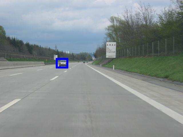
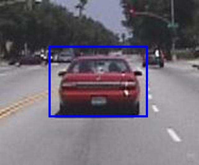
86 Figure 4.5: Successful detections on the PASCAL VOC 2005 Challenge Cars Test 1 Dataset. The last few images show multiple detection in the same image. 77

87 Chapter 5 A Discriminative Appearance Model 5.1 Introduction This chapter extends the discriminative model proposed in chapter 4 by introducing a new model for the appearance of object parts as well as modeling more general inter-part geometric constraints. The advantages of the new appearance model over the PSMs employed in the previous chapters are outlined in section The method described in this chapter represents object classes as assemblies of discriminative part models (or DPMs) obeying loose local geometric constraints. The parts are detected as parallelogram-shaped image regions and their appearance is modeled using a combination of a dense spatial pyramid histogram of gradient and edge intensities and a sparse spatial pyramid histogram of visual words. The parts are linked to enforce both geometric and co-occurrence constraints in a probabilistic graphical model (similar to chapter 4). Geometric consistency is enforced locally among nearby object parts, which allows the model to effectively prune misdetections while at the same time remain robust to viewpoint changes and within-class shape variations. Our approach allows modeling of a variety of different geometric constraints between the object parts based on their relative geometry. The final model learning problem turns out to be similar to the one obtained in chapter 4 and the appearance and geometric parameters are learned simultaneously and efficiently in a single convex optimization problem as before. 78

88 5.1.1 Motivation The appearance of the object parts was modeled using partial surface models or PSMs in chapters 3 and 4. PSMs consist of a dense, locally rigid assembly of texture patches that are allowed to deform smoothly during matching. This allows the PSMs to gain robustness to viewpoint change and non-rigid deformations. However, the PSMs are matched based using a single base training image and hence the appearance variability that they can model is restricted. We introduce a new object part model called the discriminative part model or DPM which pools together information from all the training images while learning the appearance of the part. Another important restriction of the PSMs is that the detection process works by incrementally matching small texture patches and greedily accumulating them to create the entire match. This procedure has the disadvantage that it relies on small discriminating patches to provide a correct initial estimate for the match before the match may be grown using the expansion process (of section 3.1.5). This reliance on interest point detection and repeatability decreases the generalization capability of the PSMs. The DPMs proposed in this chapter use the entire texture corresponding to the part s appearance simultaneously during the detection process. Hence, even a much smaller number of DPMs (about 1/3rd on average) can model the appearance variations for the different object parts in a complex dataset (such as the PASCAL VOC 2007 Challenge) much better than a large number of PSMs. The detection procedure is sliding window based and hence provides an appearance score for every window location instead of just providing a discrete set of detections. Also, the DPM detection process can be made extremely efficient using integral images and other ideas discussed in this chapter. On the other hand, the feature refinement process used during PSM detection makes it a much (by more than an order of magnitude) slower process. Note however that the PSMs are more robust to geometric deformations due to their flexible nature. This property allows us to match them reliably across changing viewpoints. The 79

89 DPMs can also be imparted a limited amount of invariance to viewpoint change by training them using parts imaged from different viewpoints. However, this requires an initial training set consisting of images of the part from different viewpoints. Hence, the DPM training procedure first learns PSMs from the training images and then uses the PSM detections to initialize the DPM detections to be used for training later. The inter-part relations modeled in this chapter also extend those described in chapter 4. The geometric potential is extended to allow modeling of multiple different types of inter-part relations that may exist between nearby parts. The co-occurrence potential is now included for every pair of object parts instead of only nearby parts to allow modeling self occlusion constraints for example a part on the front and a part on the rear of a car cannot be visible simultaneously. The new geometric potentials take on a simple linear form in terms of the model parameters which makes the learning process very efficient (similar to chapter 4). This chapter is structured as follows. We describe the new appearance model (the discriminative part model) for the object parts in section 5.2. The conditional random field (CRF) [50] model linking the different DPMs using specially designed interaction potentials is proposed in Section 5.3. These interaction potentials model the co-occurrence statistics and the geometric relations that exist among nearby DPMs. An efficient algorithm for learning the model parameters is described in section 5.4. The CRF model forms the basis for an effective algorithm for object detection and localization (Section 5.5). State-of-the-art results on the PASCAL VOC 2007 Challenge dataset and conclusions are presented in Section Discriminative Part Models As noted earlier, we model objects as assemblies of discriminative part models (or DPMs) that correspond to parallelogram-shaped image regions detected repeatably across a set of training images containing the object. This section explains how the appearance of DPMs 80

90 is represented in our approach, and how DPMs are learned from training data Data Preprocessing Since the objects we deal with are more or less symmetric, we learn a model to detect only objects facing to the right. The detector is run on the original image as well as its flipped version to detect both left and right facing objects. The PASCAL VOC 2007 training data contains viewpoint labels {Rear, Side, F ront} for the marked objects. We manually partition the objects with unlabeled viewpoints into two sets - the 45 o front and side viewpoint and the 45 o rear and side viewpoint to get training data for 5 different viewing directions {Rear, RearSide, Side, F rontside, F ront}. This process is similar to that used earlier for learning the PSMs DPM Initialization We begin by learning the partial surface models (or PSMs) proposed in chapter 3. These PSMs are learned using a hypothesize and validate framework as described in section 3.1. The PSM detections observed in the training data are then used to initialize the DPM detections. The DPM detections are constructed by approximating the matched regions across the training set using parallelograms and the matching transformations using affine transforms. We compute an axis-parallel bounding box B around the features constituting the PSM in the first base image. For every PSM detection m = (S,a) in the training set, we initialize the DPM detection as the parallelogram P = SB computed by projecting the bounding box B from the base image to the detection image using S. The reasons for using the PSM detections to initialize the DPM detections before learning are as follows. Firstly, since the PSMs are trained by selecting object regions that are repeatably matched across training images and are also highly discriminative, the corresponding DPMs also learn the appearance of these distinctive object parts. Secondly, as mentioned in the introduction, 81

91 since the PSMs are robust to viewpoint change, the DPM detections generated by the above process contain a good amount of viewpoint variation. This allows the learned DPMs to maintain some amount of invariance to viewpoint change as well. Apart from these PSM based parts, we also construct 5 large DPMs (one for each of the 5 different viewpoints) that cover the entire object area DPM Appearance Description Next we characterize the appearance of the matched DPM instances using a combination of two descriptors - a dense gradient and edge histogram pyramid and a sparse codebook histogram pyramid (similar to Chum et al. [13]). Dense descriptor We use the Canny edge detector to find edges in the image and extract edge components in 8 orientations (from 0 o to 180 o ). We also compute the gradient at every pixel and extract gradient components along 16 orientations (from 0 o to 360 o ). The dense descriptor is formed by constructing a hierarchical pyramid histogram (similar to Lazebnik et al. [55]) for both the Canny edges and the image gradients. An example of a histogram pyramid formed using the Canny edges is shown in figure 5.1. We allow the number of bins and pyramid levels to vary between different DPMs based on the area of the DPM relative to the object size. Larger DPMs will have a larger number of histogram bins and pyramid levels than smaller DPMs. The number of bins along the horizontal and vertical directions are chosen so that the bins are more or less square in shape and the area of the bins at the lowest level relative to the area of the entire bounding box remains more or less constant. More precisely, let α be the average ratio of the area of the DPM detections to the area of the corresponding object bounding box. We choose the descriptor dimensions at the lowest level so that the total number of bins is close to αn where N = 32 is a fixed constant across all the DPMs. The number of bins to keep along 82

92 Histogram P yramid Level 3 Image Patch Level 2 Canny Edges Level 1 Figure 5.1: Left: The image patch and the computed Canny edges. Right: The 3 level histogram pyramid of the Canny edge orientations. The lowest level is a 8 4 grid with 8 orientations from 0 to 180 o. The next level is a 4 2 grid and the highest level is a 2 1 grid. the horizontal and vertical is chosen to make the final aspect ratio of the bins close to 1. The reason why we choose to have a variable number of bins in the descriptors as opposed to keeping the descriptor dimensions fixed is explained in section The number of bins along each dimension is reduced by half when moving from a level to the next higher level. To allow for at least 2 levels in the pyramid, we always use an even number of bins along both the dimensions at the lowest level. We continue to construct the next higher level as long as the number of bins along both the dimensions at the current level is a multiple of 2. 83

93 Figure 5.2: Top discriminative codewords selected for a DPM on the side of the car. Each row shows the Hessian-Laplace features corresponding to the same codeword. Only those features that lie within the DPM are shown. Different rows correspond to different codewords. Sparse descriptor We use the Hessian-Laplace detector [73] to detect interest points in the image and describe them using the SIFT [63] descriptor. These SIFT descriptors (computed for all the training images) are then clustered using k-means into 3K visual words [89]. For every DPM, we select the 200 most discriminative codewords where the discriminability is defined as the ratio D(w) = # of occurrences of w within DPM detections # of occurrences of w in the training set. Figure 5.2 shows the the top codewords selected for a DPM on the side of the car. The sparse descriptor for a DPM is constructed as a hierarchical pyramid histogram of the selected codewords [13]. Similar to [13], each spatial bin at every level contains two different 84

94 scale bins to distinguish between features with different sizes relative to the size of the bin. Each visual word is assigned to the two scale bins using a soft assignment based on its scale. Let R be the ratio of the area of the square shaped codeword to the area of the histogram bins at a certain level. The contribution V h of the codeword to the larger scale bin is computed as follows (similar to [13]). V h = 0 if R < a (R a)/(b a) if a R b 1 if R > b. (5.1) Here, a = 0.05 and b = 0.25 are constants. The contribution V l of the codeword to the smaller scale bin is computed as V l = 1 V h. Using the above soft voting scheme instead of a hard threshold allows the descriptor to be robust to small error in estimating the scale of the Hessian-Laplace features. Note that the same detected feature may contribute to the larger scale bin on a lower level of the descriptor and to the smaller scale bin at a higher level. As with the dense descriptor, we allow the number of bins and pyramid levels to vary between different DPMs based on their sizes. The number of dimensions of the various levels are kept the same as those for the dense descriptor SVM Learning We train a support vector machine (or SVM) [12,94] to detect the DPMs based on the sparse and dense descriptors described above. Since our detection method is a scanning window based approach, it is important for the detection and classification process to be extremely efficient. Let d be the dense descriptor and s be the sparse descriptor computed on an image window. We classify the windows by constructing a linear SVM in a higher dimensional space v = [Sq(d) ; d ; s] which is quadratic in d and linear in s. The intuitive argument behind using a feature vector that is quadratic in d and linear in s is as follows. Each coordinate of the dense descriptor d is constructed a sum of the gradients or edge intensities 85

95 over all the pixels in the corresponding bin. Assuming that the variations in the gradient or edge values across the different regions of the bin to be more or less independent one can argue (using the central limit theorem [23]) that the value of the coordinates of d can be modeled by a Gaussian distribution with a fixed mean - especially for the larger bins. Projecting d into the quadratic feature space allow the learned SVM to model the constraint that d must lie close to some learned mean value. The case for the sparse descriptor s is different. Even though each bin in the sparse descriptor is again formed by summing up the contributions for the Hessian-Laplace features detected at each point in the scale space constructed within the bin, the probability that a feature corresponding to a given codeword is detected at a specific point is very small. Hence, the values of the coordinates of s are better modeled as Poisson distributions with very small mean values which can in turn be approximated as binary distributions. Hence, just using the s value in the feature vector, instead of projecting it into a higher dimensional space, is sufficient to model the relative importance of the different coordinates of s. Section 6.2 discusses how we might use other kernels (such as the Chi-Squared kernel used by Chum et al. [13]) as well. We use the efficient SV M light package provided by Thorsten Joachims [39, 40] in our implementation. We employ an incremental training strategy to train the SVM (similar to [17]). The algorithm follows the following steps. Initial training: We begin by training an initial SVM using the DPM initializations as positive examples and randomly sampled negative example windows from the background data. We also append the positive examples with deformed (slightly shifted and scaled) versions of the DPM detections in the training images. This process improves the detection performance of the DPMs by making them more robust to small deviations in the position of the detection window relative to the object part. Add hard negative examples: After training the initial SVM, we run the SVM based detector on the background images, add the resulting false positive detections 86

96 Retraining using "Hard" Negatives Detection performance Number of re training iterations Figure 5.3: The blue lines plot the detection performance of 3 different DPMs and the red line shows the average of the 3 plots. The detection performance for a DPM is computed as follows. First we choose a set of 25 validation images which contain a large instance of the object from the same viewpoint as the DPM and run the window based DPM detector on these images. Next, we compute the top 250 detection windows over this set of validation images for the DPM. Then we use each of these detections to predict a bounding box B for the object in the validation images and label the DPM detection as correct or incorrect based on whether the overlap r(b, B) between the prediction B and the actual bounding box B is greater than 0.5 (equation 3.4). The detection performance is the ratio of correct detections to the total number of detections. ( hard negative examples) to the training set and retrain the SVM. This process is repeated multiple times and helps to refine the classification boundary to better classify the difficult cases. This process was used previously (among others) by Dalal et al. [17]. Figure 5.3 shows the improvement in the part detection performance with the retraining iterations. Re-detect positive examples: Next, we run the detector in the vicinity of the original correct detections, update their position and retrain the SVM. This technique has been used previously by Chum et al. [13] and Felzenszwalb et al. [24] and helps to better align the DPMs to the part positions in the image. Add more training examples: After this, we run the detector on other images that contain the object with the same or neighboring viewpoint labels and add additional 87

97 detections as positive examples if their position relative to the corresponding object bounding boxes are similar to the other instances of the DPM. We also add detections that do not overlap with the bounding boxes or are detected at a wrong location within the bounding boxes to the set of negative examples and retrain the SVM. The output of the SVM (distance from the classification boundary) is used as the scalar appearance feature a for the next stage (Section 5.3). Fig. 5.4 shows the DPM initialization process as well as detections on multiple training images Efficient Computation over Scanning Windows Our approach requires efficient computation of the sparse and dense descriptors described above over multiple overlapping windows scanned over the image. The dense descriptor may be computed at multiple isotropic scales (where the aspect ratio of the windows is maintained across the scales) over the entire image efficiently using integral images. For efficiency, we restrict the descriptor parameters (the aspect ratio, number of histogram bins, pyramid levels) of the DPMs constructed during training to a few distinct options (about 5) to be able to reuse the same descriptor computations for detecting different DPMs in the same image. Since the integral image needs to be updated for every non-isotropic scaling, rotation or skew that we are searching over, our current system restricts the number of nonisotropic scalings that we search over to just 3 and does not search over rotations or skew for efficiency reasons. The sparse descriptor is much faster to compute since there are usually only a few (about 100 to 200) discriminative visual words selected in every image for every DPM. Hence, the sparse descriptor may be computed efficiently by looping over all these selected visual words and adding them to the corresponding bins for each of the descriptor windows they lie within. The shift between successive detection windows at a specific scale is chosen to be half the width of a single bin at the lowest layer in the DPM descriptor. The ratio between 88

98 PSM base image DP M Initialization DP M Detections Figure 5.4: The outline of learned PSM (top left) and corresponding initialized DPM (top right). Other DPM detections used for learning the appearance model (bottom). The lowest level of the pyramid is a 6x4 grid for this DPM. 89

99 successive window scales is kept fixed at 1.2 for all DPMs. The aspect ratios for the detection windows sampled are 0.8, 1.0, 1.2 times the average aspect ratio for each DPM. This sampling guarantees that there is always a detection window within a translation of 1/4 the horizontal and vertical bin dimensions and within a 10% scale from every possible true part position. We define the smallest height for the object that we are interested in detecting as H = 30 pixels. Let us use α to denote the size of the DPM relative to the object bounding box. To be able to detect the DPM for objects with heights greater than H pixels, we need to set the minimum scale at which to search for each DPM based on its size relative to the size of the entire object. Recall that we choose the number of bins in the lowest layer of the descriptors for a DPM also based on this ratio α. This ensures that the sizes of the descriptor bins at the lowest search scale for the DPMs are more or less similar across the different DPMs. This in turn makes the number of descriptor windows to be sampled also more or less the same for the different DPMs. If we were to use a fixed number of bins for every DPM instead of varying them according to the DPM s relative size we would need to sample smaller DPMs more densely than larger DPMs. Computing detections from SVM responses: We employ a simple scheme to compute a set of DPM detections from the responses of the window based SVM detector. We consider the windows (with SVM score greater than a threshold β = 0) in the order of their SVM score and keep adding them to the set of DPM detections as long as they do not lie within a specific range (in position, scale and skew) of any of the previously selected detections. These selected DPM detections are then used in the CRF framework to compute geometrically consistent sets of DPMs - corresponding to object instances in the image. 5.3 Geometric Model The object is modeled as a set of DPMs with geometric and co-occurrence constraints imposed between the DPMs. If the object is present in the image some of these DPMs may 90

100 be detected at different locations within the image. Hence, each object DPM u may either be associated with a specific DPM detection or may be absent in the image (possibly due to occlusion). We represent a DPM detection as a parallelogram shaped region in the target image. 1 Hence, it may be characterized by a 6 dof affine transformation that maps the DPM from a canonical coordinate frame to the parallelogram detection in the target image. We represent the detection variable x i corresponding to DPM u i as a triple x i (o, S, a). The three components of the triple are defined below: Occlusion o: The binary variable o {vis, occ} defines the visibility/occlusion state of the DPM u in the image. If u is detected in the image o = vis and if u is not detected (possibly due to occlusion) o = occ. Location S: If o = vis, the location variable S corresponds to the affine transformation that takes the DPM from its position in a canonical coordinate frame to the parallelogram shaped detection patch where it was detected in the target image. Appearance a: If o = vis, the appearance a is the single real valued output of the SVM based DPM detector. The detection variables defined above are similar in spirit to those defined for the PSMs in chapter 4. Let us define X as the set {x 1,...x m } of all the detection variables for the m different DPMs in the model. The framework used to model the geometric constraints described in this chapter is similar in spirit to framework proposed in chapter 4 to model inter- PSM relations. In particular, we again model the conditional probability distribution over different DPM detections X given the observed image I as a conditional random field [50]. Using (as before) the Hammersley Clifford theorem [8] and assuming only the pairwise clique potentials to be non-zero, P(X I) can be decomposed as 1 As mentioned before, our current system does not search over rotations and skew for efficiency reasons and so the DPM detections are just rectangular regions with variable aspect ratios. We however describe the model in the general case of parallelogram detections. 91

101 P(X I) = 1 Z exp A i (x i,i) + xi X I ij (x i, x j,i) (x i,x j ) E where Z is the normalization constant, A i (x i,i) is the association potential and I ij (x i, x j,i) is the interaction potential as before. As in chapter 4, we represent both the association potential A i (x i,i) and the interaction potential I ij (x i, x j,i) as linear functions of feature vectors. More precisely, we will define A i (x i,i) = αi T h i (x i,i) and I ij (x i, x j,i) = βijg T ij (x i, x j,i), where h i (x i,i) and g ij (x i, x j,i) are feature vectors and α i and β ij are parameters of the model. As before, the conditional log likelihood of the labeled training examples becomes convex in the model parameters in this case. We now describe the association and interaction potentials employed in our method Association Potential The association potential A i (x i,i) measures how likely it is (based only on appearance) that the detection associated with x i (o i, S i, a i ) is a correct DPM detection. If o i = occ, we model A i (x i,i) as a constant value zero. If o i = vis, we model A(x i,i) as a linear function of the appearance score a returned by the SVM. The association potential can be written as A i (x i,i) = αi T h i (x i,i), where α i is a 2 dimensional parameter vector corresponding to DPM u i and, [a i ; 1] if o i = vis h i (x i,i) = 0 2 if o i = occ Interaction Potential The interaction potential I ij (x i, x j,i) encodes the interaction between the detections variables x i (o i, S i, a i ) and x j (o j, S j, a j ) corresponding to the DPMs u i and u j. If either of o i or o j is occ, the interaction potential takes the constant value zero. If both o i and o j are 92

102 vis, the interaction potential consists of the following components: Pairwise co-occurrence potential This potential models the correlation between the occurrences of the different DPMs in an object. It is important for two reasons: 1) to model the correlation between nearby and overlapping object DPMs and 2) to model the self occlusion constraints between pairs of DPMs (for example, the constraint that the front and rear of a car cannot be visible simultaneously). The co-occurrence potential between two DPMs u i and u j may be represented as Iij c = ρ ij gij(x c i, x j,i), where ρ ij is a parameter of the model and the co-occurrence feature gij(x c i, x j,i) is defined as 1 if o gij(x c i = vis and o j = vis i, x j,i) = 0 o/w. The pairwise co-occurrence potential above is similar the the co-occurance potential used in chapter 4 but in the current method this potential is used for all pairs of DPMs instead of only between the nearby DPMs. Local geometric potential This potential models the geometric relation between nearby object DPMs. The potential is specially designed to allow modeling two different types of inter-dpm relations based on their relative geometry. Let the detection variables corresponding to two linked DPMs be x i = (o i, S i, a i ) and x j = (o j, S j, a j ). We represent the 6 parameter relative affine transformation T ij = Si 1 S j as a column vector t ij of length 6. More precisely, t ij contains the 6 entries from T ij in row-major order. 1. Geometric consistency between DPMs on a single smooth surface: As argued in chapter 3, the relative affine transformation among nearby parts on the same smooth surface is robust to viewpoint change. We can model this constraint using a potential 93

103 T ij Canonical Frames u i u j Target Image Figure 5.5: Inter-DPM geometric consistency for nearby DPMs on a single smooth surface. that takes the quadratic form τ ij γij{sq(t T ij µ ij )} and hence prefers configurations where the 6 parameters t ij of the relative affine transformation remains close to some mean value µ ij. This potential is similar to the geometric potential used in chapter 4. Hence as before it can be written as a linear function of a quadratic feature vector v ij constructed from t ij as v ij = [Sq(t ij ) ; t ij ; 1]. 2. Geometric consistency between DPMs on two intersecting smooth surfaces: This is the type of constraint that would connect a DPM on the front of a car to one on the side of the car. Since we do not model the 3D angle between the DPM surfaces and the camera orientation explicitly, we cannot completely constrain the exact position of one DPM detection relative to the other like in the previous case (6 constraints on T ij ). However, any point p (in the image) on the intersection curve of the two surfaces must 94

104 be consistent with both S i and S j since it lies on both the surfaces. Let p i (resp. p j ) be the projection of p into the canonical frame of S i (resp. S j ). Then S i p i = p = S j p j and hence p i = T ij p j. Imposing this constraint for all the points on the intersection curve C (which may be approximated by a line l in the vicinity of the nearby DPMs) provides us with 4 independent constraints on T ij. More precisely, let p i + λd i (respectively, p j + λd j ) be points on the line in the canonical frame of S i (respectively, S j ) that correspond to the points p + λd in the image. Then, λ, S i (p i + λd i ) = p + λd = S j (p j + λd j ). This implies λ, p i + λd i = T ij (p j + λd j ). (5.2) We may model this constraint using a potential of the form π ij ωij T {Sq(T ijp j p i )} νij T {Sq(T ijd j d i )}. This potential is general enough to be able to model the constraint that T ij p j must remain close to p i and that T ij d j must remain close to d i. Using simple algebra, we can equivalently write this potential as special case of a more general linear function of a vector of features constructed from t ij. In particular, we can write it as a linear function of the feature vector b ij where, b ij = [Sq(t ij ) ; Cr(t ij (1 : 3)) ; Cr(t ij (4 : 6)) ; t ij ; 1]. (5.3) The notation Cr(v) denotes the vector consisting of the all the cross terms v(i)v(j) for all i j. Note that this linear function has more degrees of freedom than required to model the constraint in equation 5.2. We choose to learn the potential in this form because the potential is now a linear function of the feature vector b ij which is 95

105 T ij p i p j Canonical Frames l C u i p u j Target Image Figure 5.6: Inter-DPM geometric consistency for nearby DPMs on two intersecting smooth surfaces. important to keep the learning problem convex. 3. Geometric consistency between DPMs attached at a single point: This type of constraint connects parts that are attached at a single point but can move around freely otherwise. An example would be the geometric constraint between the parts on the legs of a cow and its body. This constraint can be modeled in a similar way to the case with two intersecting surfaces. Let p be the point in the image where the two surfaces are attached. Also, let p i and p j be the projections of p into the canonical frames of S i and S j. As before we require S i p i = p = S j p j which in turn implies p i = T ij p j. As described above, we model this constraint using a potential which is a linear function of the feature vector b ij described in equation

106 The final geometric potential takes a general form and allows modeling all three of the above constraints. If o i = occ or o j = occ, the geometric potential I g ij (x i, x j,i) takes on a constant zero value. If o i and o j are both vis, the geometric potential is modeled as a linear function of a quadratic feature vector b ij (from equation 5.3. Hence, we may represent the geometric interaction potential as I g ij (x i, x j,i) = ηijg T g ij (x i, x j,i) where, g g ij (x b ij if o i = vis and o j = vis i, x j,i) = 0 19 o/w. The interaction potential I ij (x i, x j,i) is just the sum of the geometric potential I g ij (x i, x j,i) and co-occurrence potential Iij(x c i, x j,i). Note that the co-occurrence potential is defined for all pairs of DPMs whereas the geometric potential is only defined for DPMs that occur in the vicinity of each other and is zero for all other DPM pairs. Also note that the form of the geometric potential subsumes the co-occurrence potential for the DPM pairs where is it defined. Because of this, we may combine the geometric and co-occurrence potentials into a single linear form I ij (x i, x j,i) = βijg T ij (x i, x j,i) where g ij (x i, x j,i) is either g g ij (x i, x j,i) or gij c (x i, x j,i) depending on whether the two DPMs u i and u j are nearby or not. 5.4 Parameter Learning Using the expressions for the association potential and the interaction potential defined in Section 5.3, we may write the probability P(X I) of the detection variables X given all the DPM detections observed in I as ) P(X I) = 1 Z exp ( i α T i h i(x i,i) + i,j β T ij g ij(x i, x j,i). We call an instance of the object detection variables X observed in an image an object 97

107 instance configuration (or OIC). For learning the CRF model, we require a set of training images {I 1...I T } labeled with their OICs {X 1... X T }. Since it is not possible to manually label the OICs in the training data, we use an automatic process to generate this labeling (similar to chapter 4). We run the SVM based DPM detectors on all the training images and label each DPM detection as either correct or incorrect based on whether it lies within a specific range relative to the object bounding box (similar to chapter 4). The detection variable x i associated with a correct detection is set to be x i (vis, S i, a i ) where S i is the location and a i is the appearance value (SVM output) of the detection. The detection variables for the DPMs which do not correspond to any correct detection are set to (occ,, ) 2. As in section 4.3, if a training image contains multiple objects, we break it into multiple training cases (multiple OICs) - each corresponding to a single object within the image where all the correct DPM detections corresponding to all the other objects are marked as incorrect. Let Λ be the set of all the model parameters: the α i s and β ij s in the association and interaction potentials. We are interested in finding the Λ that maximizes the conditional likelihood of all the observed OICs (automatically constructed above) given all the detections ( T ) in the training images. That is, we want to find Λ = argmax Λ t=1 P(X t I t ). Since the exponent in the CRF model is linear in the parameters (similar to chapter 4), the conditional likelihood of the correct detections in the training images is convex in the model parameters (see Appendix B) Gradient Approximation for Learning Let f(x) P(x) denote the expectation of f(x) under the probability distribution P(x). The gradient of the conditional log-likelihood with respect to the parameter vectors α i and β ij in the CRF model can be written as: 2 Note that we can set S i and a i to any value for a detection variable x i which has o i = occ. This does not influence the learned model since the likelihood is independent of S i and a i when o i = occ. 98

108 0 x 104 Conditional log likelihood Cummulative step length Figure 5.7: Evolution of the pseudo conditional log likelihood during gradient ascent learning of the model parameters on the PASCAL VOC 2007 dataset (car class). L = [ ] hi (x t i α,it ) h i (x i,i t ) P(xi I t ), i t T L = [ gij (x t i β, xt j,it ) g ij (x i, x j,i t ) P(xi,x j I )] t ij t T where T is the set of training images. Computing the exact marginals P(x i I t ) and P(x i, x j I t ) in the above expressions is intractable because our CRF is a complete graph. Hence, as was done in chapter 4, we replace the exact marginals with pseudo-marginal approximations that can be computed by running loopy belief propagation on the CRFs for each training example. The details of the belief propagation algorithm were described in section A simple gradient ascent procedure with an adaptive step length using this approximate gradient is used to maximize the convex conditional log likelihood function. Figure 5.7 shows the evolution of the pseudo-conditional log likelihood during the optimization process. 99

109 5.5 Object Detection The object detection process uses a similar approach to the procedure described in section 4.4. We begin by detecting the DPMs in the test image I using the SVM based detector to get a set of possible DPM detections D. For detecting an object we are interested in finding the most likely OIC X (or set of OICs {X 1... X k } - for multiple objects) given the observed detections D in I. To compute the most likely OIC, we run the iterated conditional modes (or ICM) algorithm [9] on the CRF. The ICM algorithm is initialized with an OIC where all the detection variables x i are initialized to (occ,, ) and iteratively updates them to their optimal values based on the current values of the neighboring detection variables in the CRF. This converges to a locally optimal OIC X. To detect multiple object instances within an image we remove the detections selected in X from D and rerun the ICM algorithm on the CRF for the remaining detections to generate the other object instances. Each OIC X is scored by considering the sum of the appearance scores a i for each of the DPMs u i visible 3 in X. Each visible detection x i (with occlusison state set as vis) within X can be used predict a bounding box for the object based on its mean position relative to the bounding boxes in the training images for the DPM. The final bounding box prediction is computed as the weighted (according to a i ) average of the bounding box predictions for each visible DPM u i in X. 5.6 Experimental Results We have evaluated our approach on the car, cow and motorbike categories in the PASCAL VOC Challenge 2007 dataset. We chose these categories since the dataset consists of a large number of images for these categories and many other state-of-the-art methods have reported results on these categories. The challenge test set consists of a total of 4952 test 3 A DPM u i is visible in an OIC X iff the occulsion variable in x i is vis. 100

110 Algorithm Car Cow Motorbike Our Method Chum et al. [13] Felzenszwalb et al. [24] INRIA Plus [20] IRISA [20] INRIA Normal [20] MPI ESSOL [20] Figure 5.8: Comparison of average precision (AP) scores with other top performing methods on the PASCAL VOC 2007 dataset. The scores in bold represent the best performance for the class. images containing the object instances in varying poses and at multiple different scales. Some qualitative detection and localization results of the proposed method are shown in Figure 5.10, Figure 5.11 and Figure The proposed approach is able to detect instances of the object with significant intraclass variation in appearance and from varying viewpoints. The PASCAL VOC 2007 Challenge uses the same average precision (or AP) measure described in section to compare the different methods. Figure 5.8 compares our method s AP with other top performing methods. Our precision recall curves for the three datasets are shown in Fig As mentioned in Section 5.2, we manually partition the training images with unlabeled viewpoints into two viewpoint classes - 45 o rear and side, and 45 o front and side. The comparisons are thus slightly biased in our favor since the other methods did not have this extra annotation. This viewpoint information allows us to correctly label the DPM detections in the training images as correct or incorrect (as described in Section 5.4) before learning the CRF model parameters. 101

111 1 PASCAL VOC2007 CAR, AP = PASCAL VOC2007 COW, AP = Precision Precision Recall 1 PASCAL VOC2007 MBIKE, AP = Recall Precision Recall Figure 5.9: Precision-Recall curves for the car, cow and motorbike datasets. 102

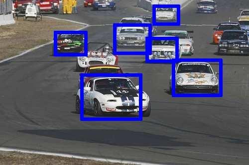
112 Figure 5.10: Some detection results on cars. The last two rows of detections show a few failures of the model. The red bounding boxes show mis-detections - some of these correspond to unlabeled objects, others are caused due to similarity in appearance. Some of the object instances are missed by the system because they are smaller than the minimum search scale of the part detectors or because they are imaged from viewpoints not used during training (the last image). 103

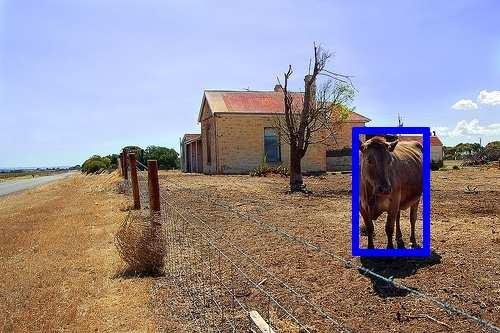
113 Figure 5.11: Some detection results on cows. The last two rows of detections show a few failures of the model. The red bounding boxes show mis-detections - some of these correspond to objects labeled as difficult, which are ignored in the evaluation. Other mis-detections are caused due to similarity in appearance. Some of the object instances are missed by the system because they are smaller than the minimum search scale of the part detectors or because they involve variations in the shape of the object due to articulation (the last image) 104

114 Figure 5.12: Some detection results on motorbikes. The last two rows of detections show a few failures of the model. The red bounding boxes show mis-detections - some of these mis-detections are caused due to similarity in appearance. Some of the object instances are missed by the system because they are smaller than the minimum search scale of the part detectors or because they are imaged from viewpoints not used during training (the last image). 105

115 Chapter 6 Conclusions and Future Directions This thesis proposes a number of different multi-viewpoint probabilistic part based models for object detection. All the models consist of two main components - 1) a model for the appearance of the parts and 2) a model for the inter-part relations. The models proposed are robust to viewpoint change both at the part detection stage as well as at the inter-part geometric modeling stage. In this chapter we summarize the contributions of this thesis and outline some directions for future work. 6.1 Contributions Chapter 3 describes an appearance model (termed as a partial surface model or PSM) to characterize the appearance of an object part. A PSM models an object part as a dense collection of texture patches - some of which are primary interest points detected by a feature point detector [41] and others are general secondary texture patches. These texture patches are linked locally to allow smooth deformations in their geometric structure. Chapter 3 described the algorithms to automatically learn PSMs from training images and to detect them in other images. The key advantage of using PSMs in a multi-viewpoint detection system is that the local consistency enforced during feature matching makes them more flexible and robust to viewpoint variations. Chapter 3 also describes a Markov random field based model (the PSM graph, section 3.3) 106

116 for modeling the relative geometry of the different PSMs that make up the object. The nodes of the PSM graph correspond to the learned PSMs and the links between them constrain the relative affine deformations in nearby PSMs. Again, employing only local geometric constraints makes the model robust to viewpoint variations. Chapter 4 introduces a new discriminative approach to model the inter-part geometry and co-occurance relations. The new model is based on the conditional random field (CRF) framework and does away with various restrictive independence assumptions imposed by the generative model proposed in chapter 3. In particular, the appearance of the parts are no more considered independent from each other and from the geometric relations between the parts. Chapter 4 also provided a simple and efficient algorithm for learning the parameters of the CRF model. Finally, in chapter 5 we introduce a discriminative appearance model for the object parts (termed the discriminative part model or DPM). Though the PSMs used in chapter 3 and chapter 4 are designed to be robust to viewpoint variations they suffer from a lack of generalization capacity due to the fact that their appearance is based on a single training image. To improve generalization performance DPMs learn an SVM classifier to detect the object parts from a training set consisting of all the observed detections of the object part in the training set. The DPMs use a specially designed feature vector consisting of a dense edge and gradient histogram pyramid and a sparse histogram of codewords corresponding to image features to describe the object parts. An efficient sliding window based detector is then employed to detect occurrences of the DPM in a target image. Chapter 5 also extendes the inter-part geometric model (CRF) proposed in chapter 4 to allow more accurate modeling of the different types of inter-part geometric relations including those between the parts on different object surfaces. Algorithms for efficiently learning the model parameters are also provided in chapter

117 6.2 Future Directions In this section we briefly mention some promising directions for extending the work presented in this thesis. A key advantage of the discriminative part model or DPM over the PSMs is that it provides an appearance score for every window location on the image instead of only at a sparse set of detections. We can use this score to define a continuous appearance based density over the 6 dimensional space of possible DPM detections in the image. This can allow for using the appearance and geometric information simultaneously while detecting the object parts. In particular, the original DPM detections generated as described in chapter 5 could be refined using the geometric CRF model to simultaneously maximize the joint appearance and geometric probability of the configuration of object parts. As mentioned in section 5.2.4, we may look to improve DPM detection performance by employing a non-linear kernel for comparing the pyramid of histogram based features. Popular kernels for recognition and scene classification tasks include the histogram intersection kernel of Grauman and Darrel [42] and Lazebnik et al. [55], and the chi squared kernel used by Bosch et al. [11], Varma and Ray [95] and Chum and Zisserman [13]. The problem with using a non-linear kernel is the associated computational cost - classifying each image patch would now require s kernel computations where s is the number of support vectors in the corresponding SVM as opposed to a single dot product in the linear SVM case. One could use a hierarchical approach where a linear SVM is used to throw away 90% of the image region as not containing the object part and later a non-linear SVM is used to select the final detections from the promising regions returned by the linear SVM. The PASCAL VOC Challenge datasets do not contain the viewpoint labels for the 45 o 108

118 viewpoints. To have a better comparison with other competing approaches one could look at ways to automatically partition the objects into the two viewpoint classes (as well as determine whether the objects is facing to the right or to the left) by clustering descriptors computed over the entire object area. The geometric location of the front, side and rear DPMs detected on the objects in the training images can also be used to help with the partitioning. 109

119 Appendix A Non-linear Match Refinement In this chapter, we describe the non-linear match refinement algorithm used during PSM learning and matching in chapters 3 and 4. We can represent each feature match between two parallelogram shaped image features as m = (S, T ) where S represents the matching region in the first image I 1 and T represents the corresponding region in the second image I 2. The match refinement algorithm works by computing the optimal deformation of the parallelogram T in I 2 that maximizes the correlation between the descriptors D(S) and D(T ) for the two matching regions. This process is used to correct the initial alignment of matching image patches. The first patch S is kept fixed throughout the refinement process. We want to compute, [ T = argmax D(S) T D(T ) ]. (A.1) T In this thesis, we employ the 128 dimensional SIFT descriptor (of David Lowe [63]) to describe the patches being matched. The non-linear minimization is performed using the Levenberg-Marquardt (LM) optimization algorithm [59, 67]. The LM algorithm interpolates between the Gauss-Newton algorithm [78] and the method of steepest descent. When the current solution is far from the correct one, the algorithm behaves like a steepest descent method. On the other hand, when the current solution is close to the correct solution, it becomes a Gauss-Newton method. Since the algorithm is standard, we omit the details here. 110

120 Rothganger et al. [85] employ a similar match refinement procedure where they maximize the normalized cross correlation between the intensity values of the matched patches. In [85], the authors assume that the intensity is a smooth function over the matching patches and compute the Jacobian analytically. This is much harder in our case since we use the SIFT descriptor instead of the intensity values directly. Hence, we use a numerical approximation to the Jacobian. Our implementation uses the Levenberg-Marquardt minimization package - Levmar [62] provided by Manolis Lourakis. Figure A.1 shows the intermediate steps during the refinement of a match. 111

121 Matching Second Image Patch T First Image Patch S Refinement Figure A.1: Non-linear match refinement: The patch S in the first image I 1 (left). The evolution of the matching patch T in the second image I 2 during the refinement (right columns). A large error in alignment for the original match is corrected by the refinement procedure. The initial match with the large alignment error was created by deforming the matching region T of an interest point match detected between the two images. 112