State Space Model of a Light Weight Flexible

Transcription

1 State Space Model of a Light Weight Flexible Telescope A Thesis Presented to the Faculty of California Polytechnic State University, San Luis Obispo In Partial Fulfillment of the Requirements For the Degree of Master of Science In Mechanical Engineering By Chi-Yeh Hsu August 2010

2 2010 Chi-Yeh Hsu All Rights Reserved ii

3 Committee Membership Title: State Space Model of Light Weight Flexible Telescope Author: Chi-Yeh Hsu Date Submitted: August, 2010 Committee Chair: Dr. John Ridgely Assistant Professor Cal Poly Mechanical Engineering Committee Member: Dr. Charles Birdsong Associate Professor Cal Poly Mechanical Engineering Committee Member: Dr. Xi Wu Assistant Professor Cal Poly Mechanical Engineering iii

4 Abstract State Space Model of a Light Weight Flexible Telescope Chi-Yeh Hsu The accuracy of optical telescope in the past was dominated by the construction of the telescope body and the precision of optical surface. This thesis fits into a larger project with a goal of controlling a flexible telescope in order to help a cheaper telescope achieve higher accuracy. In order to understand the internal motion of telescope, the goal of this thesis is to build a state space model of a two-degree-of-freedom telescope using a known star location as feedback. The model presented in this thesis may be used for the telescope simulation and the control design in the future. This project considers a light weight flexible structured telescope and uses state space formulation to model dynamic motion of the telescope since state space model is better for modeling and analyzing a multiple-inputs and multiple-outputs system. A onedegree-freedom experimental test stand is built to generate a series of telescope motion data in order to examine whether the telescope simulation model can represent a real telescope system. To record the telescope motion, a wheel encoder mounted on the azimuth motor and a LED light density sensor installed at the end of telescope body are used as feedbacks. The results show that the state space model can simulate many system dynamic behaviors as shown in the experimental result; however, it is not feasible to obtain all of telescope s physical parameters from the system feedbacks. iv

5 Table of Contents List of Figures... vii List of Tables... viii List of Equations... ix Chapter 1: Introduction : Background : Star Tracking and Telescope Control Altazimuth Tracking : Open Loop and Closed Loop Position Control : Disturbances : Stability Criteria : Project Overview and Objective Chapter 2: Model of Flexible Telescope : Telescope System : Structure Components : Control Inputs : Sensor Feedback : Model of External Disturbances : Gravity : Wind : Azimuth System : Model of Azimuth System : Azimuth Model State Equations : State space Model of Azimuth System : Altitude System : Model of Altitude System : Altitude Model State Equations : State space Model of Altitude System : Matlab Simulation : Simulink Model : Simulation Output Chapter 3: Azimuth Experimental Telescope v

6 3.1: Experiment Set Up : Telescope Structure : Software and Data Acquisition Interface : Guide Star Feedback Simulation : Experiments Result : Light Feedback : PI Control : Tap Test : Feedback Control Using Light Feedback Chapter 4: Simulation Result Analysis : Turned Simulation model : PI Control Tuning : Frequency Response of Simulation Model : Controllability and Observability Analysis Chapter 5: Conclusion : Light Weight Flexible Telescope Model : Experimental Test Stand : Control Analysis : Current Project State and Future Work Reference Appendix A: Derivation of Azimuth Model Appendix B: Disturbance Model Appendix C: Derivation of Altitude Model Appendix D: Matlab Simulation Model Appendix E: Matlab Plot Functions Appendix F: OTA Calculation Appendix G: System Parameters vi

7 List of Figures Figure 1: Stationary Telescope Hooker telescope at Mount Wilson Observatory... 2 Figure 2: Homemade telescope... 3 Figure 3: Altitude (h) and Azimuth (A) coordination... 5 Figure 4: Telescope Open Loop Control flow chart... 7 Figure 5: Telescope Closed Loop Control flow chart... 8 Figure 6: Generalized Telescope System Figure 7: Telescope System Components Figure 8: Azimuth Telescope Model Figure 9: Azimuth Telescope Model Tree Diagram Figure 10: Star Image Displacement Figure 11: Altitude Telescope Model Figure 12: Altitude Telescope Model Tree Diagram Figure 13: State space subsystem Figure 14: Wind model for altitude system Figure 15: Gravity model Figure 16: Full telescope in Simulink Figure 17: PID controller Figure 18: Result of azimuth simulation Figure 19: Result of altitude Simulation Figure 20: pointing path and star image feedback Figure 21: Experimental Setup of experimental telescope Figure 22: Motomatic Station Figure 23: SC 2075 DAQ Interface Figure 24: Simulated Star Source Figure 25: Star Image senor used on Test Stand Figure 26: Star image feedback simulation sensor situation Figure 27: Light response from Simulation Figure 28: Telescope test Figure 29: Star Image feedback reading Figure 30: Telescope control response (PID control) Figure 31: OTA response to tap test Figure 32: Frequency response of telescope to tap test Figure 33: PI control using star image feedback Figure 34: Turned Simulation Result Figure 35: Frequency response of simulation model vii

8 List of Tables Table 1: Telescope system components Table 2: Control Inputs of telescope Table 3: Sensor Feedback of telescope Table 4: Modeling Parameters for Azimuth Model Table 5: Modeling parameters for Altitude Model (Part1) Table 6: Modeling parameters for Altitude Model (Part2) Table 7: Natural frequency of components Table 8: Controllability and Observability Analysis viii

9 List of Equations Equation 1: Gravitational disturbance Equation 2: Wind disturbance Equation 3: States of azimuth system Equation 4: State space equation of azimuth model Equation 5: Torque transformation of azimuth model Equation 6: Transformed azimuth model States Equation 7: Transformed state equation for azimuth model Equation 8: State Space Model for Azimuth Equation 9: Azimuth Model Input Equation 10: Azimuth Model Output Equation 11: Star Image Displacement Calculation Equation 12: Reduced Star Image Displacement Equation Equation 13: Azimuth Model disturbance Source Equation 14: State (A) matrix for azimuth model Equation 15: Input (B) matrix for azimuth model Equation 16: Output (C) matrix for azimuth model Equation 17: Direct transmittance (D) matrix for azimuth model Equation 18: Disturbance (E) matrix for azimuth system Equation 19: States of altitude system Equation 20: State equation of altitude system Equation 21: Torque transformation of altitude model Equation 22: Altitude Model State Equation 23: Transform state equations for altitude model Equation 24: State Space Model for Altitude Equation 25: Altitude Model Input Equation 26: Altitude Model Output Equation 27: Star Image Displacement Calculation for altitude model Equation 28: Reduced Star Image Displacement Equation of altitude model Equation 29: Altitude Model Disturbance Source Equation 30: System (A_a) matrix for altitude model Equation 31: Input (B_a) matrix for altitude model Equation 32: Output (C_a) matrix for altitude model Equation 33: Direct transmittance (D_a) matrix for altitude model Equation 34: Disturbance (E_a) matrix for altitude model ix

10 Chapter 1: Introduction 1.1: Background The accuracy of optical telescopes in the past time was dominated by the construction of the telescope body and the precision of optical surface. In order to have an accurate optical telescope, the telescope must have an extremely rigid and heavy structure. The rigid telescope body can decrease structure deformation under external disturbances. A heavy telescope structure can help reduce vibration caused by impulse disturbance and telescope tracking motion. This kind of telescope (Shown in Figure 1) is stationary and constructed inside a shelter which makes it free from many environment disturbances. Moreover, the gear ratio in the drive chain is big in order to support and control heavy telescope structure; therefore the tracking motion is very slow. 1

11 Figure 1: Stationary Telescope - Hooker telescope at Mount Wilson Observatory 1 The FEA (Finite Element Analysis) model is a popular method for structure modeling for big telescopes. However, it is hard to design a control system using FEA model generated by a computer due to its complicated and usually oversized model. This kind of telescope control heavily relies upon empirical data. Each telescope is tested. Data Results are used to create a LUT (Lookup Table). The LUT includes the amount deformation occurs on the telescope structure under external disturbances. This LUT is be used as reference for control calibration.[1] Some other telescope, because of its need to move and operate at different location, is constructed with a much lighter structure. An amateur 1 Source: Photograph Andrew Dunn, 1989.< 2

12 telescope is an example of it (Shown in Figure 2). This kind telescope is required to be disassembled and moved to a remote location, usually outdoors. The operator will put it together at the location. The light structure telescope is susceptible to structure vibration and external disturbances. The first reason is that the maximum weight of the telescope is limited by the transportation tool and human power that put it together. Due to this weight limit, the construction of telescope isn t as stiff and heavy as stationary telescope. Second, a light structure telescope is usually operated in an environment with more external disturbances. Since there is no shelter or dome to protect it, disturbances like wind or a wild animal can directly affect the telescope. Figure 2: Homemade telescope 2 Besides being susceptible to vibration and deformation, it is also hard to calibrate a light structure telescope. Even though the telescope calibration 2 Source: amateur telescope making < > 3

13 strategy using empirical data is common for a big stationary telescope, the same method is less useful for the light structure telescope. This is because of the uncontrollable environment and errors in the set up process. The telescope structure will be slightly different every single time. The calibration process is also time consuming and requires many precise measuring tools. It isn t feasible to perform it on a low price telescope every time an operator sets it up. On the other hand, modern telescopes have additional sensors. Many of these sensors could provide extra information about the telescope. Moreover, a high torque motor could be used as a direct drive motor on a light structure. The drive chain could be eliminated since the inertia of such a telescope is low. It ers a faster response and a more linear system. With the faster computer used today, it is possible to apply active control with additional feedback to improve performance of a light structure telescope. 1.2: Star Tracking and Telescope Control Altazimuth Tracking Many light structure telescopes are manual operated telescope. It requires the operator to manually point it at the target star. Since the star actually travels across the sky over night, the operator also needs to adjust its pointing so the target star will stay in the field of view. Some telescopes are computer controlled so it can track a single star over the sky in a long period of time. Two main 4

14 tracking strategies are used today. 1. Altazimuth Mounts 2. Equatorial Fork Mounts Altazimuth method uses two motors with position control to control the azimuth and altitude of the telescope. The altitude and azimuth system is the coordination used to describe the pointing direction of telescope. Altitude and azimuth coordination is shown in Figure 3. In this figure, h represents altitude angular position. Altitude is measured as the angle from horizontal to the direction which the telescope pointing and it goes from 0 degrees to 180 degrees. "A" represents the azimuth angular position. Azimuth is measured as the angle from north of the direction of the telescope is pointing from a horizontal plane and it goes from 0 degrees to 360 degrees. These two values can fully define the telescope point in a half-sphere above the horizon. Figure 3: Altitude (h) and Azimuth (A) coordination 5

15 Altazimuth tracking is used for the telescope system discussed in this project since it is used by most of research telescopes and amateur telescopes today. Altazimuth tracking is more mechanically complicated compared to equatorial tracking. The equatorial tracking has a rotational axis parallel to the Earth s axis of rotation; hence it only needs to rotate about one single axis at a constant speed to follow a star in the sky. The Altazimuth tracking requires two axes, azimuth and altitude, to track a star over the sky. Two axes have to continually move at a different rate in order to track a celestial target. However, equatorial tracking requires a massive and precise mounting structure in order to make sure it is parallel to the Earth s axis of rotation. For an amateur, it is easier and cheaper to construct a two axes system than design a heavier and more expensive equatorial mount. The complex control issue can usually be solved by the integration of a microcontroller or computer controlled system : Open Loop and Closed Loop Position Control The open loop position control indicates that the telescope doesn t know where the star is [2]. It only knows which direction it is pointing. The open loop position control uses position sensors on the telescope rotation axis to measure the pointing angle. In the case of the Altazimuth mount, there is one encoder on each axis (Shown in Figure 4). These sensors are used to measure drive motor angular displacement. Then control system can calculate the altitude angle and azimuth angle of the telescope. Most of light structure telescope uses this 6

16 method to track a star. Figure 4: Telescope Open Loop Control flow chart However, a telescope using an open loop control doesn t know if it is actually pointing at the target star. The vibration and deformation in the OTA (Optical Telescope Assembly) affects telescope pointing. They create errors that are not observable by the position sensors placed on the end of a drive chain. Though position sensors suggest that the telescope is pointing at the correct direction; the combined angular position, telescope pointing direction plus deformation of OTA, might not be correct. Most of stationary telescopes use empirical data to calibrate the control system. This method adds or subtracts a certain amount of an angle when the telescope is at a different location. For example: if the telescope is trying to aim at a star at a 24 degrees altitude, the LUT fixes it to 26 degrees. Two extra degrees is compensated for telescope deformation due to gravity. This method is also not feasible to a light structure telescope due to cost of time and precise tools. It also does not help compensate for external disturbance that is not repeatable. Close loop position control uses the star as a feedback signal. The star sensor forms a second feedback loop (Shown in Figure 5). This method uses a star image sensor to measure the displacement of a reference star (a 7

17 bright, not-interfered star at known location is usually picked as reference star because it gives clearer location feedback) from where it is supposed to be. This information can be used for fine adjustment of telescope pointing. Since it is using an observed target as its feedback source, this method makes sure that the combined angular position is correct. Control Signal Controller Motor Position Sensor Telescope Human Eye or Sensor Motor Position Feedback Star Sensor Star Image Feedback Figure 5: Telescope Closed Loop Control flow chart 1.2.3: Disturbances Gravity produces repeatable deformation [2]. The effect of gravity on the telescope is due to the deformation of the telescope structure. The deformation is always in the vertical direction. OTA deformation due to gravitation is a function of the altitude angular position. If the altitude is small, the telescope will have a bigger deformation. Gravitational disturbances only exist in an altitude model. It won t affect the telescope motion on a horizontal plane. Wind produces non-repeatable deformation [2]. The disturbance caused by wind has a slow and fast component. The slow component of wind disturbance is the steady wind. It applies a long and steady force on the telescope structure and causes the telescope to drift away from its target. 8

18 The steady wind is usually large in amplitude and could cause large telescope deformation. However, behavior of steady wind is usually more predictable. The fast component of the wind disturbance is wind gust. The wind gust is characterized by an abrupt and nearly discontinuous force on telescope body. However, the amplitude of wind gust is smaller and doesn t create as much deformation as a steady wind. The gust is usually 20% to 10% of steady wind [3]. The steady wind information can be monitored by an external weather station or observed using a feedback star image. The wind gust acts like noise from the environment. Due to gust s short time constant, it is hard to observe it from a weather station and is usually observed through a star feedback system. The telescope model models the wind as a torque applied on the motor shaft. The amplitude of the torque caused by steady wind is a function of wind disturbance amplitude, wind direction, and the position of telescope at the moment. If the telescope structure is perpendicular to the wind direction, the effect of the wind is the biggest. The steady wind source is modeled by a square wave. The wind gust is white noise with amplitude equal to 20% to 10% of the square wave [3]. Like the wind, temperature also produces non-repeatable deformation. The change of temperature which affects telescope accuracy occurs on a rather long time; this is because the sudden change of air temperature usually has small amplitude and the telescope component usually has a large thermal time constant; therefore, the small temperature change usually won t change telescope geometry. The large temperature change which affects 9

19 telescope geometry occurs on a time scale of hours and days. Since the project focuses on the transient response, the telescope model does not count for the temperature in the environment. Other disturbances include human contact, atmosphere air density change, ground vibration, and other light pollution. The accidental touching of the telescope structure can be modeled as a stronger wind gust. Other effects generally have less amplitude comparing with major disturbance and are ignored in the current model : Stability Criteria The response of telescope to control input and environmental disturbances changes the direction of telescope pointing. For a stable telescope, this change of pointing needs to remain in tolerance over a certain length of time. If the change of the angular pointing direction is too big, the star image will become blurring. The tolerance is determined by the observation target. The change of the angular pointing direction should not change by more than 1/10 of the beam s width. The equation is Δθ θ /10 ( λ/ D)/10 [2]. λ is wavelength of observation target and D is the main reflector diameter. The pointing stability is determined by the structure of the telescope. 10

20 1.3: Project Overview and Objective Modern telescope is an integrated mechanical and electrical system. Its accuracy is challenged by telescope structure and external disturbances, as gravity, wind, and temperature change. Another issue is the internal friction in the telescope system. The internal friction is an issue for a light weight flexible telescope because this kind of telescope is not as well constructed as a VLT (very large telescope). It takes the telescope extra effort to overcome the static friction when it starts moving and usually causes an overshoot. It is hard to design a high performance control system for a light weight flexible telescope. Its light structure makes it susceptible to vibration and deformation. It is easily disturbed and usually operated under many environmental disturbances. Most importantly, many techniques used to calibrate research telescope can t be used on an individual telescope. In order to design a control system, it is important to gain a better understanding of the telescope system. Many of light structure telescopes are custom-build and modified for the user. Each of them has distinct structure characteristics, and therefore a specific model does not help too much. This project describes a light structure flexible telescope as a generalized flexible telescope structure. It fits into a larger project with a goal of controlling a flexible telescope in order to help a cheaper telescope achieve higher accuracy. The model of a flexible telescope provides a telescope dynamic in state-space format since state space model is better for modeling and analyzing a multiple inputs and multiple outputs system. The model includes a transient flexible 11

21 response in order to represent the telescope response to a control input or a disturbance. It models the telescope tracking motion but also the vibration of each vibrating elements. In this case, it is important that the model can demonstrate the first vibration mode and simulates pointing error of the telescope since the first vibration mode causes the greatest pointing error of the telescope tracking. This model also models environment disturbance. Gravity and wind is considered in the model. The model concentrates on modeling the transient response of telescope. The effect of temperature change is not considered since its time constant is a lot longer. The goal of this project is to construct a model for a light weight flexible telescope serving as a platform for testing active control system and system identification. In order to exam that if the telescope simulation model can represent a real telescope system, a one degree freedom experimental test stand is built to generate a series of telescope motion data. The simulation model is not a dynamic model for this experimental test stand; however, the model should be able to reproduce many system patterns shown in the experimental data since the general shape of simulation model and experimental is the same. The simulation of an experimental test stand is analyzed to determine the controllability and observability of the system. It shows the minimum requirement of sensor feedbacks in order to enable the operator to capture all the major and minor motion during the telescope motion. 12

22 Chapter 2: Model of Flexible Telescope This chapter presents the modeling of the light weight flexible telescope mechanical and electrical system. The telescope structure consists of azimuth motor, altitude motor, telescope fork, OTA (Optical Telescope Assembly), mirror(main reflector), and mirror mount. The telescope electronics includes two driving motors. This model also counts control inputs used to perform telescope tracking and possible external disturbances that affect telescope performance. 2.1: Telescope System Figure 6: Generalized Telescope System To model the motion of a flexible telescope, a general shape 13

23 telescope with Altazimuth tracking system is considered (shown in Figure 6). The cylindrical body on the top is the body of telescope. It contains the OTA, the main reflector (mirror), and the mirror mount. The bottom part is the telescope mount. It contains the fork, two driving motor, and all the controller components. The generalized telescope model, without flexibility, is a system with two degree of freedom. The telescope rotates around two axes. Azimuth motion rotates around Z-axis and altitude motion rotates around X-axis. Two axes intersect at center of gravity of telescope body; therefore, without disturbance, the telescope should be a stable system which can stay still at any position : Structure Components The generalized telescope mechanical system has five major components (Shown in Figure 7 and Table 1). Red dot on Figure 7 is the center of gravity and the rotational center of the telescope body. Mirror mount is the rear end of the telescope body which holds telescope mirror. OTA extends out from the mirror mount. The observing point is at the opposite end of the OTA, illustrated with a green dot on the Figure 7. The fork is the entire supporting mount of the telescope. When models a telescope mechanical system, two motor and drive chain is part of the fork. The fork, OTA and the mirror mount together is the telescope structure. 14

24 Figure 7: Telescope System Components Two motors are the electrical-mechanical system. They convert electric current in the electrical system into torque. Azimuth motor and altitude motor provide torque to two axes of telescope mechanical system. The generalized telescope uses direct drive motor; therefore, there is no gear chain between telescope axes and motor. They change angle between telescope body and telescope mount. These two motor receive control input from the position controller. Table 1: Telescope system components Parts Azimuth Motor Altitude Motor Fork OTA Mirror and Mirror Mount Description Motor that controls azimuth motion of telescope Motor that controls altitude motion of telescope The stand of telescope; support OTA and lift it from the ground Front part of telescope body, from where fork contacts with body to where image receiver is Rear part of telescope body, from where fork contacts with body to where primary mirror is 15

25 2.1.2: Control Inputs Control inputs are part of the electric system of the telescope. The generalized telescope control system has two inputs (shown in Table 2). Telescope control inputs are generated by the position controller. These two voltage signals are sent to the power amplifier. The amplified signals are sent to the motor and used to control motor output. Table 2: Control Inputs of telescope Input Type Azimuth Motor Altitude Motor Description Voltage input, controls azimuth motion Voltage input, controls altitude motion 2.1.3: Sensor Feedback Telescope systems have three different sensor feedbacks (shown in Table 3). First two sensors are azimuth encoder and altitude encoder. In a generalized telescope model, they are considered as ideal position feedback sensors which give motor angular position in radius with an infinite small resolution. They are directly connected to the motor. Since there is not gear chain in the mechanical system, the outputs are also an angular position of general telescope pointing direction. The feedbacks from encoders are illustrated by an arrow between position sensor and position controller. The star image sensor is mounted on the extended end of OTA. Its location is illustrated with the green dot in Figure 7. In the generalized telescope model, the output of star image sensor is the displacement between desired 16

26 telescope pointing center and combined pointing center, which also counts for the fork, OTA, and mirror mount vibration. It produces a 2 degrees displacement on XY coordination. The feedback from the star image sensor is illustrated by arrow between the reflectors/receivers and the position controller. In the generalized model, the sensor images a reference star that is always at the actual center of telescope pointing; therefore, always provides a feedback. In a real system, the star image feedback only works when the reference star is in the field of view, which means the telescope open loop controller has to be able to bring the telescope pointing direction close to the reference star location before the star image sensor starts to work. Table 3: Sensor Feedback of telescope Feedback Type Azimuth encoder Altitude encoder Star image Description Gives angular position and angular velocity in azimuth direction Gives angular position and angular velocity in altitude Gives target star location in XY coordination 2.2: Model of External Disturbances 2.2.1: Gravity The gravitational disturbance is modeled as torque applied on the altitude model. Gravitational torque is a function of telescope length, telescope pose, and the mass of instrument mounted on the end of upper OTA and mirror mount. The calculation is shown in Equation 1. 17

27 Equation 1: Gravitational disturbance T = min t g Cos( θ ) L Gravity s rument axis telescope The angular position change of the telescope in the altitude system is from 0 to 90 degrees; therefore, the torque is nonlinear. The torque is calculated externally from the system model and brought in the model as input. Gravitational disturbances caused by the OTA and the mirror mount should balance each other since the telescope is a balanced system. However, gravitational force still bends the OTA and the mirror mount slightly hence create a star image displacement : Wind The wind disturbance is modeled as torque applied on both the altitude and azimuth model. The pressure from the wind force is P = 0.5ρ V C [6]. V w 2 wind air w is the speed of wind and C is the shape factor of the telescope body. C is assumed to be 1 in this project since the true shape of telescope is unknown. From wind pressure, the torque applied on rotational center of telescope is calculated by multiplying the wind pressure by the telescope section area and half of the length of the telescope (shown in Equation 2). Equation 2: Wind disturbance T V Cos Sin Area L 2 wind = 0.5 ρair [ win d ( θj θwind ) θj ] telescope 0.5 telescope The angular position change of the telescope is 0 o 90 degree in the 18

28 altitude system and 0 to 360 degree in the azimuth system; therefore, the torque is nonlinear. The torque is calculated externally from the system model and brought in the model as input. 2.3: Azimuth System Generalized telescope model is separated into two parts: azimuth model and altitude model. The azimuth and the altitude system is treated as uncoupled in current model; however, in a real telescope there are some coupling between those axes. One of the coupling sources is the gyroscopic effect. Nevertheless, the telescope is usually operated under low speed with very low rotational angular acceleration; therefore, coupling between two subsystems can be ignored. The azimuth model describes telescope motion around Z axis, and the altitude model describes telescope motion around X axis : Model of Azimuth System Structure components of azimuth model include azimuth motor, OTA, mirror mount, and Fork. In the azimuth model, the altitude model is considered part of the fork. The relationship between each structure component is shown in Figure 8. The springs and dampers shown in the figure are torsional springs and torsional dampers. The azimuth motor is connected to the ground which provides absolute zero reference for the angular velocity of mechanical system. The azimuth system has one control input. When input voltage is sent to azimuth 19

29 motor, rotor A will gain velocity while velocity of rotor B will be zero. The angle between rotor A and rotor B is ϴ J. A rotational spring and damper connects rotor A and the fork/altitude motor. The angular position of the fork is ϴ Jam. This angular position is the absolute angular position, the angle between the fork and ground zero (North). The fork/altitude is connected to the mirror mount and OTA with two separated rotational springs and damper sets. When the fork/altitude motor displaces, torque will be sent to the mirror mount and OTA through the spring and damper set; therefore, moving mirror mount and OTA. The entire system will move with the input from the azimuth motor. The angular position of OTA is ϴ O and angular position of mirror mount is ϴ m. The detail parameters for azimuth model are shown in Table 4) 20

30 Table 4: Modeling Parameters for Azimuth Model Azimuth Model Parameters Description Unit J Inertia of azimuth control motor kg m J O Inertia of OTA 2 2 kg m 2 J m Inertia of mirror mount kg m 2 J f Inertia of fork and altitude motor kg m K O Spring of OTA around z axis in horizontal direction N m / radius Spring of mirror mount around z axis in horizontal K m N m / radius direction K f Spring of fork around z axis in horizontal direction N m / radius B Damping coefficient of azimuth control motor N m s / radius B O Damping coefficient of OTA in horizontal direction N m s / radius Damping coefficient of mirror mount in horizontal B m N m s / radius direction B f Damping coefficient of fork around z axis N m s / radius R Internal resistance of azimuth motor system Ω L Internal inductance of azimuth motor system H K Motor constant of azimuth motor system N m/ Amps a States Description Unit θ J Angular position of azimuth pointing Radius θ J O Angular position of OTA Radius θ J m Angular position of mirror mount Radius θ J f Rotation angle of fork and altitude motor around z axis Radius Ω J Azimuth angular velocity of azimuth pointing Radius / s Ω J O Azimuth angular velocity of OTA Radius / s Ω J m Azimuth angular velocity of mirror mount Radius / s Ω J f Azimuth angular velocity of fork and altitude motor Radius / s i L Current through azimuth control motor Amps Source Description Unit V s Input voltage for azimuth control motor V Disturbance Description Unit T s1 Wind disturbance act on OTA for azimuth model N m T s2 Wind disturbance act on mirror mount for azimuth model N m Output Description Unit θ J Angular position of azimuth as output Radius ΩJ Azimuth angular velocity Radius X Guide star feedback sensor for azimuth coordination Radius t 21

31 2.3.2: Azimuth Model State Equations Figure 8: Azimuth Telescope Model Graphical technique is used to represent the dynamics system model [5]. The linear graph represents the topological relationships of lumped-element interconnections within system [5]. Linear graph of azimuth model is shown in Figure 9. This graph is used represents both the electrical and mechanical system. The loop on the left is the model of DC motor. The bigger loop on the right is the model of the telescope mechanical system. The component connecting the two systems is electric mechanical component motor. The motor serve as a transformer in between two loops transfer current (shown as 1 on Figure 9) to torque (shown as 2 on Figure 9). From the linear graph, the system has 8 states (Shown in Equation 3). 22

32 Equation 3: States of azimuth system X = ΩJ, ΩJam, ΩJo, ΩJm, TKf, TKo, TKm, i L Figure 9: Azimuth Telescope Model Tree Diagram Eight state variables are used to generate 8 state equations to represent dynamic motion in the azimuth system (Shown in Equation 4). The detail derivation is shown in Appendix A. 23

33 Equation 4: State space equation of azimuth model dω J 1 1 = [ il B Ω J TKf Bf ( Ω J Ω Jam)] dt J K a dω Jam 1 = [ TKf + Bf ( Ω J Ω Jam ) TKo Bo ( Ω Jam Ω Jo ) TKm Bm ( Ω Jam Ω Jm )] dt J am dω Jo 1 = [ TKo + Bo ( Ω Jam Ω Jo ) + Ts 1 ] dt J O dω Jm 1 = [ TKm + Bm ( Ω Jam Ω Jm ) + Ts 2 ] dt J m dil 1 1 = ( Vs RiL ΩJ) dt L Ka dtkf 1 = ( ΩJ Ω Jam) dt J dt dt Ko dt dt Km am 1 = ( ΩJam ΩJo ) J O 1 = ( ΩJam ΩJm ) J m Four states TKf, TKo, T Km shown in Equation 3 are hard to be measured in the azimuth system with accessible sensors. However, it is easier to transform them into a different format. Torque between two components can be rewritten as angular displacement multiplied by the rotational spring constant (Shown in Equation 5). Equation 5: Torque transformation of azimuth model T T T ( θ θ ) ( θ θ ) ( θ θ ) = K Kf f J Jam = K Ko O Jam O = K Km m Jam m Azimuth model states have now become angular positions and angular 24

34 velocities of system components and current in the electric system. New azimuth models states is shown in Equation 6. With the new state variables, state equation is transformed also. New state equation is shown in Equation 7. Equation 6: Transformed azimuth model States θj θ Jam θ JO θjm Χ= Ω J ΩJf Ω JO Ω Jm i L 9X 1 25

35 Equation 7: Transformed state equation for azimuth model dθj =ΩJ dt dθjam =ΩJam dt dθjo =ΩJo dt dθjm =ΩJm dt dω J 1 1 = [ il B Ω J K f( θj θjam) Bf( Ω J Ω Jam)] dt J K dω Jam 1 = [ K f ( θj θjam ) + Bf ( Ω J Ω Jam ) Ko ( θjam θjo ) Bo ( Ω Jam Ω Jo ) Km ( θjam θjm ) dt J am B ( Ω Ω )] a m Jam Jm dω Jo 1 = [ Ko ( θjam θjo ) + Bo ( Ω Jam Ω Jo) + Ts1] dt J O dω Jm 1 = [ Km ( θjam θjm ) + Bm ( Ω Jam Ω Jm ) + Ts 2 ] dt J m dil 1 1 = ( Vs RiL ΩJ) dt L Ka 2.3.3: State-space Model of Azimuth System 8 states variables are the minimum set of variables which can be used to describe azimuth system. System outputs are system variables that are accessible and can be measured by the sensors (shown in Equation 10). There are 3 system outputs we can obtain from sensors. They can generate 3 output equations. 8 state variables are substituted with 9 state variables. These 9 state equations and output equations are rewritten in state-space format (shown in Equation 8). 26

36 Equation 8: State Space Model for Azimuth Χ= A Χ + B U + E d Y = C Χ + D U 9X9 9X1 9X1 1X1 9X2 2X1 3X9 9X1 3X1 1X1 The system input of azimuth model is voltage sent to the electric system (Shown in Equation 9) Equation 9: Azimuth Model Input U = [ V s ] 1 X 1 There are 3 system outputs. Angular position and angular velocity of the motor could be obtained from azimuth encoder. X t is the output from the star image sensor. It is the displacement of the reference star. Equation 10: Azimuth Model Output θj Y = ΩJ X t 3X 1 X t is a function of mirror mount angular position and OTA angular position of the azimuth system (shown in Figure 10). Angular displacements of the OTA and the mirror mount both create image displacements. The star image displacement is a combination of these two displacements. This relationship is listed in Equation 11. Using small angle approximation, Equation 11 can be linearized into a simpler format (shown in Equation 12). Notice the term θ Jam is canceled in the equation. Vibration of fork does not affect azimuth pointing. 27

37 Figure 10: Star Image Displacement Equation 11: Star Image Displacement Calculation X = L sin{2[( θ θ ) + ( θ θ )] L sin[( θ θ ) + ( θ θ )] t OTA Jm Jam Jam J OTA Jo Jam Jam J Equation 12: Reduced Star Image Displacement Equation X = L θ L θ + 2L θ t OTA J OTA Jo OTA Jm There are two disturbance sources in the azimuth model. The wind torque applied on OTA and the wind torque applied on mirror mount. In azimuth motion, wind effect on fork is small; therefore, it is ignored. Equation 13: Azimuth Model disturbance Source d T s1 = T s2 2X 1 All system matrices can be determined by transformer 9 state equations and 3 output equations. System matrices are shown below. A matrix shown in Equation 14 is the state matrix of the azimuth system. 28

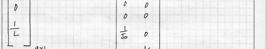
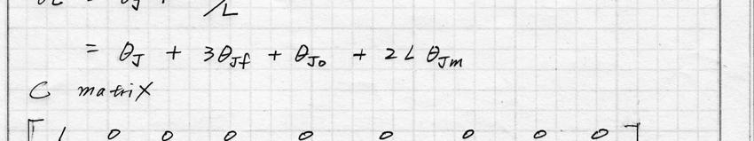
38 Equation 14: State (A) matrix for azimuth model ( KO + Km) KO Km ( B+ BO + Bm) B BO B 1 m 0 J J J J J J J KaJ K f B ( B+ Bf ) J f J f J f KaJ f KO KO BO BO JO JO JO J O Km Km Bm Bm Jm Jm Jm J m 1 1 R KL a KL a L 9x9 B matrix shown in Equation 15 is the input matrix of the azimuth system. Equation 15: Input (B) matrix for azimuth model L 9X 1 C matrix shown in Equation 16 is the output matrix of the azimuth system. 29

39 Output variables θ J and calculated using Equation 12. ΩJ is a direction output from state variables. X t is Equation 16: Output (C) matrix for azimuth model X 3 9 D matrix shown in Equation 17 is the direct transmittance matrix for the azimuth model. In the azimuth system, input of the system doesn t affect outputs; therefore transmittance matrix is a zero matrix. Equation 17: Direct transmittance (D) matrix for azimuth model X 1 system. E matrix shown in Equation 18is the disturbance matrix for the azimuth 30

40 Equation 18: Disturbance (E) matrix for azimuth system JO 1 0 Jm 0 0 9X 2 2.4: Altitude System Altitude model describes the telescope motion around the X axis : Model of Altitude System The structure of the altitude model is similar to the azimuth model. Components include altitude motor, OTA, mirror mount, and Fork. In the altitude model, the azimuth model is considered part of the ground. The relationship between each structure component is shown in Figure 11. The springs and dampers shown in the figure are torsional springs and torsional dampers. In the altitude model, the fork is connected to the ground which provides absolute zero reference for the angular velocity of mechanical system. The altitude motor sits on the top of the fork and provide torque source to all 3 other components. The altitude system has one control input. When input voltage is sent to the altitude 31

41 motor, both rotor A, which is connected to mirror mount and OTA, and rotor B, which is connected to the fork will gain velocity. The angle between rotor A and rotor B of altitude motor isθ Ja. Rotor B is connected to the fork and has the same angular displacement as fork ϴ f.. Since the fork is connected to the ground, the angular displacement of rotor B is limited by the spring element of fork. The altitude motor is connected to the mirror mount and OTA with two separated rotational spring and damper sets. When altitude motor displaces, torque will be sent to mirror mount and OTA through the spring and damper set; therefore, moving mirror mount and OTA. The OTA and mirror mount move with rotor A of the altitude motor. The angular position of fork oscillates and goes to zero. The angular position of OTA is θ O_ aand angular position of mirror mount is θ m_ detail parameters for azimuth model are shown in Table 5 and table 6. a. The 32

42 Table 5: Modeling parameters for Altitude Model (Part1) Altitude Model Parameters Description Unit J Inertia of altitude control motor kg m _ a J Inertia of OTA O_ a J Inertia of mirror mount m_ a J Inertia of fork f _ a O_ a 2 2 kg m 2 kg m 2 kg m K Spring of OTA around z axis in vertical direction N m / radius K Spring of mirror mount around z axis in vertical direction N m / radius m_ a K Spring of fork around z axis in vertical direction N m / radius f _ a B Damping coefficient of altitude control motor N m s / radius _ a B Damping coefficient of OTA in vertical direction N m s / radius O_ a B Damping coefficient of mirror mount in vertical direction N m s / radius m_ a B Damping coefficient of fork around y axis N m s / radius f _ a R _ a Internal resistance of altitude motor system Ω L _ a Internal inductance of altitude motor system H K Motor constant of altitude motor system N m/ Amps a_ a States Description Unit θ J _ a Angular position of altitude point Radius θ J O_ a Altitude angular position of OTA Radius θ J m_ a Altitude angular position of mirror mount Radius θ J f _ a Altitude angular position of fork around z axis Radius Ω J _ a Altitude angular velocity of altitude point Radius / s Ω J O_ a Altitude angular velocity of OTA Radius / s Ω J m_ a Altitude angular velocity of mirror mount Radius / s Ω Altitude angular velocity of fork Radius / s J f _ a i Current through altitude control motor Amps L_ a Source Description Unit V s _ a Input voltage for altitude control motor V Disturbance Description Unit T s1_ a Wind disturbance act on OTA for altitude model N m T s2_ a Wind disturbance act on mirror mount for altitude model N m T s3_ a Wind disturbance act on fork N m T s4_ a Torque from gravitational force on OTA N m T Torque from gravitational force on mirror mount N m s5_ a 33

43 Table 6: Modeling parameters for Altitude Model (Part2) Altitude Model Output Description Unit θ J _ a Angular position of altitude as output Radius Ω J _ a Altitude angular velocity Radius Y Guide star feedback sensor for altitude Radius t_ a 2.4.2: Altitude Model State Equations Figure 11: Altitude Telescope Model Graphical technique is used to represent dynamics system model [5]. Linear graph represent the topological relationships of lumped-element interconnections within system [5]. Linear graph of altitude model is shown 34

44 in Figure 12. This graph is used represents both the electrical and mechanical system. The loop on the left is the model of the DC motor. This part is identical to the azimuth system. The bigger loop on the right is the model of the telescope mechanical system. It is different with azimuth due to its different structure. The component connecting the two systems is electric mechanical component motor. The motor serve as a transformer in between two loops transfer current (shown as 1 on Figure 12) to torque (shown as 2 on Figure 12). From the linear graph, the system has 8 states (Shown in Equation 3). These 8 states are used to generate 8 state equations to represent dynamic motion in the azimuth system Equation 19: States of altitude system X = Ω, Ω, Ω, Ω, T, T, T, i J _ a Jf _ a Jo_ a Jm_ a Kf _ a Ko_ a Km_ a L_ a Eight state variables are used to generate 8 state equations to represent dynamic motion in the altitude system (Shown in Equation 20). The detail derivation is shown in Appendix B. 35

45 V = 0 Ω=0 Figure 12: Altitude Telescope Model Tree Diagram 36

46 Equation 20: State equation of altitude system dωj _ a 1 1 = [ i B ( Ω Ω ) T B ( Ω Ω ) T dt J K _ a a_ a B ( Ω Ω )] m_ a J _ a Jm_ a L_ a _ a J _ a Jf _ a Ko_ a o_ a J _ a Jo_ a Km_ a dωjf _ a 1 1 = [ il_ a+ B_ a( ΩJ _ a ΩJf _ a) TKf _ a Bf _ aω Jf+ Ts3] dt J K dω Jo _ a dt dω Jm _ a dt Kf _ a Ko _ a Km _ a f _ a a_ a 1 = [ TKo _ a + Bo _ a ( ΩJ _ a Ω Jo _ a ) + Ts 1_ a + Ts 4_ a ] J _ a O_ a 1 = [ TKm + Bm _ a ( ΩJ _ a Ω Jm _ a ) + Ts 2_ a + Ts 5_ a ] J m_ a dil_ a 1 1 = ( Vs RiL ( ΩJ _ a ΩJf _ a)) dt L Ka dt dt dt dt dt dt 1 = Ω J f _ a O_ a m_ a Jf _ a 1 = ( ΩJ _ a ΩJo_ a ) J 1 = ( ΩJ _ a ΩJm_ a ) J T, T, T Four states _ Kf a Ko a Km a shown in Equation 19 are hard to be measured in the altitude system with accessible sensors. However, it is easier to transform them into a different format. Torque between two components can be rewritten as angular displacement multiplied by the rotational spring constant θ (Shown in Equation 21). f defines angular displacement of fork; therefore, torque in fork is only a function of θ f K and f. 37

47 Equation 21: Torque transformation of altitude model T T T = K θ Kf _ a f _ a f _ a ( θ θ ) ( θ θ ) = K Ko_ a O_ a J _ a O_ a = K Km_ a m_ a J _ a m_ a Altitude model states have now became angular positions and angular velocities of system components and current in the electric system. Altitude models states is shown in Equation 22. With the new state variables, state equation is transformed also. New state equation is shown in Equation 23. Equation 22: Altitude Model State θ θ θ θ Ω J _ a Jf _ a JO _ a Jm _ a Χ= J _ a Ω Ω Ω i Jf _ a JO _ a Jm _ a L_ a 9X 1 38

48 Equation 23: Transform state equations for altitude model dθj _ a =ΩJ _ a dt dθjf _ a =ΩJf _ a dt dθjo _ a =ΩJo _ a dt dθjm _ a =ΩJm _ a dt dωj _ a 1 1 = [ il_ a B_ a( ΩJ _ a ΩJf _ a) Ko_ a( θj _ a θjo_ a) Bo_ a( ΩJ _ a ΩJo_ a) dt J K _ a a_ a K ( θ θ ) B ( Ω Ω )] m_ a J _ a Jm_ a m_ a J _ a Jm_ a dωjf _ a 1 1 = [ il_ a+ B_ a( ΩJ _ a Ω Jf _ a) K f _ aθ Jf _ a Bf _ aω Jf + Ts3] dt J K dω Jo _ a dt dω Jm _ a dt _ a f _ a a_ a 1 = [ Ko_ a ( θj _ a θjo_ a ) + Bo_ a ( ΩJ _ a Ω Jo_ a ) + Ts 1_ a+ Ts4_ a ] J O_ a 1 = [ Km_ a ( θj _ a θjm_ a ) + Bm_ a ( ΩJ _ a Ω Jm_ a ) + Ts2_ a+ Ts5_ a ] J m_ a dil_ a 1 1 = ( Vs RiL ( ΩJ _ a ΩJf _ a)) dt L Ka 2.4.3: State-space Model of Altitude System 8 states variables are the minimum set of variables which can be used to describe the altitude system. System outputs are system variables that are accessible and can be measured by the sensors (shown in Equation 26: Altitude Model Output). There are 3 system outputs we can obtain from sensors. They can generate 3 output equations. 8 state variables are substituted with 9 state variables. These 9 state equations and output equations are rewritten in statespace format (shown in Equation 24). 39

49 Equation 24: State Space Model for Altitude Χ = A Χ + B U + E d _ a _ a9x9 _ a9x1 _ a9x1 _ a1x1 _ a9x5 _ a5x1 Y = C Χ + D U _ a _ a3x9 _ a9x1 _ a3x1 _ a1x1 The system input of altitude model is voltage sent to the electric system (Shown in Equation 24). Equation 25: Altitude Model Input U = Vs_ a 1X 1 There are 3 system outputs. Angular position and angular velocity of motor could be obtained from altitude encoder. Y t_ a is the output from star image sensor. It is the displacement of reference star. Equation 26: Altitude Model Output Y θ = Ω Y J _ a J _ a t_ a 3X 1 Y is a function of mirror mount angular position and OTA angular t_ a position of the azimuth system (shown in Figure 10). Its relation is listed in Equation 27. Using small angle approximation, Equation 27 can be linearized into a simpler format (shown in Equation 29). The equation is different with the azimuth model. Fork vibration affects altitude pointing.\ 40

50 Equation 27: Star Image Displacement Calculation for altitude model Y = L sin{2[( θ θ ) + θ ] L sin[( θ θ ) + θ ] t_ a OTA Jm_ a J _ a Jf _ a OTA Jo_ a J _ a Jf _ a Equation 28: Reduced Star Image Displacement Equation of altitude model Y = L θ + L θ L θ + 2L θ t _ a OTA J _ a OTA Jf _ a OTA Jo _ a OTA Jm _ a There are five disturbance sources in the altitude model (Shown in Equation 29). The wind torque applied on OTA, the wind torque applied on mirror mount and the wind torque applied on the fork. Another two disturbances are gravitational disturbance on OTA and mirror mount. Equation 29: Altitude Model Disturbance Source d T T T s1_ a s2_ a = s3_ a T T s4_ a s5_ a 5X 1 All system matrices can be determined by transformer 9 state equations and 3 output equations. System matrices are shown below. A_a matrix shown in Equation 14 is the state matrix of the altitude system. 41

51 Equation 30: System (A_a) matrix for altitude model ( KO_ a+ Km_ a) KO_ a Km_ a ( B_ a+ BO_ a+ Bm_ a) B_ a BO_ a Bm_ a 1 0 J J J J J J J K J K f _ a B_ a ( B_ a + Bf _ a) J J J K J KO_ a KO_ a BO_ a BO_ a JO_ a JO_ a JO_ a JO_ a Km _ a Km_ a Bm_ a Bm_ a Jm_ a Jm_ a Jm_ a Jm_ a 1 1 R_ a Ka_ al_ a Ka_ al_ a L_ a _ a _ a _ a _ a _ a _ a _ a a_ a _ a f _ a f _ a f _ a a_ a f _ a 9x9 B_a matrix shown in Equation 31 is the input matrix of the altitude system. Equation 31: Input (B_a) matrix for altitude model L _ a 9X 1 C_a matrix shown in Equation 32 is the output matrix of the altitude system. Output variables θ J _ a and ΩJ _ a is a direction output from state variables. Y is calculated using Equation 28. t_ a 42

52 Equation 32: Output (C_a) matrix for altitude model X 3 9 D_a matrix shown in Equation 33 is the direct transmittance matrix for the altitude model. In the altitude system, input of the system doesn t affect outputs; therefore the transmittance matrix is a zero matrix. Equation 33: Direct transmittance (D_a) matrix for altitude model X 1 system. E_a matrix shown in Equation 18is the disturbance matrix for the altitude 43

53 Equation 34: Disturbance (E_a) matrix for altitude model J f JO J O Jm J m X 5 2.5: Matlab Simulation 2.5.1: Simulink Model In order to simulate the telescope motion, the state-space formulas are imported into Simulink. A state space subsystem is built for handling the state space formula. The state-space subsystem is shown in Figure 13. This subsystem integrates the change rate of last step and adds the saved current state position. This forms the current state position. The current position and input are used to calculate the change rate of the current step and then import into the next step. 44

54 Figure 13: State-space subsystem Gravity disturbances and wind disturbance is calculated with environmental wind speed and states of telescope. Because of the models are nonlinear, they are calculated externally in a different subsystem and imported into the state-space loop as disturbance inputs. Gravity model is shown in Figure 14. Wind model for altitude is shown in Figure

55 Figure 14: Wind model for altitude system Figure 15: Gravity model The full flexible telescope simulator is shown in Figure 16. It consists of a two state-space handler for the azimuth system and the altitude system and a disturbance model. Disturbance model includes gravity model and two wind models for the azimuth model and the altitude model. A complete set of 46

56 telescope Simulink model can be found in Appendix C. Disturbance model takes wind direction, wind speed and telescope pose from state variables as input. It generates seven disturbance outputs and sent to the azimuth and the altitude model. Figure 16: Full telescope in Simulink Two PID controllers are added into the system to perform position feedback control using angular position outputs from the azimuth model and the altitude model. PID control is shown in Figure

57 Figure 17: PID controller 2.5.2: Simulation Output The result from the simulation is saved in Matlab. There are three Matlab plotting functions for handling a saved result. Plot_Function_Azimuth.m is used to plot azimuth motion. The result is shown in Figure 18. The top plot on the left shows the telescope point at the rotational axis. The mid plot on the left shows feedback from star sensor, which represents the combination telescope pointing. The bottom plot on the left shows the control input sent to telescope. Three plots on the right shows vibration of fork, OTA and mirror mount of azimuth system. The vibration is defined as difference between component angular position and main telescope pointing direction. 48

58 Figure 18: Result of azimuth simulation Plot_Function_Altitude.m is used to plot altitude motion. The result is shown in Figure 19. It plots same information as azimuth motion. 49

59 Figure 19: Result of altitude Simulation Plot_Function_2Axis shows displace on two main axes and feedback on star image sensor. This information is actually observable to the control system. It also plots the change path of combined telescope pointing direction and star image feedback on XY coordination during telescope motion. The result is shown in Figure 20. The detail plotting function can be found in Appendix E. 50

60 Figure 20: pointing path and star image feedback The telescope pointing direction from the image feedback sensor shows a higher frequency motion than the pointing direction obtained from encoder. This is because the image feedback sensor also reflects the vibration in the OTA and the mirror mount. 51

61 Chapter 3: Azimuth Experimental Telescope In order to verify the simulation, a one degree of freedom experimental telescope is built to generate a set of experimental data. The simulation parameters are adjusted so that the simulation result can reassemble this experimental data. 3.1: Experiment Set Up 3.1.1: Telescope Structure The experimental test stand reproduces the azimuth model. The telescope experimental test stand is shown in Figure 21. The frame of experimental test stand is considered as part of the ground and not considered in the model. A Pittman motor with an E60 encoder is mounted at the bottom plate between two beams of the frame. The telescope body, composited of long steel plates, is mounted between the top and bottom plates. In order to reduce fiction, two shaft adapters are manufactured using the CNC machine to mount the telescope body. The main reflector is taken down from an ORION telescope StarBlast 4.5. Its diameter is 113 mm and has a focal length of 450 mm. 52

62 Figure 21: Experimental Setup of experimental telescope Analog output from the controller is amplified using the MOTOMATIC Station used for Cal Poly, San Luis Obispo mechanical engineering ME 422 control class (Shown in Figure 22). The power amplifier saturated at 3 amps output. The green LED on the MOTOMATIC station turns red when power the amplifier is saturated. The power amplified has a gain of 5.25 V/V. Derivative control is not used because the resolution of the E60 encoder attached to the Pittman motor is low. E60 encoder has 1024 pulses per revolution. Its accuracy is only 0.35 degree. Derivation of feedback error becomes infinite when encoder increment. This produces a high frequency noise in output signal when the telescope runs at high speed and produces a nonlinear system behavior during low speed. This behavior cause instability of telescope test stand; therefore, derivative gain is set to 0 for position controller of 53

63 experimental test stand. Figure 22: Motomatic Station 3.1.2: Software and Data Acquisition Interface The experimental is controlled using a position control with PI feedback controller. The controller is constructed using Simulink. Control signals are generated by SC-2075 DAQ Interface (Data Acquisition Interface). SC-2075 DAQ interface is shown in Figure 23). This DAQ interface connects to an internal National Instrument E-Series DAQ card. The controller uses a bidirectional counter embedded in the E-Series DAQ card to determine the angular displacement of motor. Current position controller used for the system is a single input single output controller. It takes either motor encoder reading or the star image sensors reading as input, and sends an analog signal as output. The output is connects to 54

64 power amplifier input on the MOTOMATIC station. Figure 23: SC-2075 DAQ Interface 3.1.3: Guide Star Feedback Simulation The star source is simulated with a 100W light bulb. The feedback sensor is most sensitive to infrared and red light; therefore an incandescent lamp is used for this experiment. The simulated source is shown in Figure

65 Figure 24: Simulated Star Source Figure 25: Star Image senor used on Test Stand Light from the simulated source shines on the mirror and is reflected to the sensor placed close to focal point of the mirror. The star image sensor is simulated with two LED set next to each other. The distance between the two LED is adjusted so it is the same as the diameter of source light. An instrument amplifier is used to take the differential between voltage outputs of LED sensors. When the light shines on LED, the LED generates an electric current according to the intensity of the light shines on it. A light sensor used on the test stand is shown in Figure 25. The star feedback is shining on the right LED on this figure. 56

66 Figure 26: Star image feedback simulation sensor situation Figure 26 shows the layout of the LED sensor. At part (A), the light source shines at the center of two sensors. Two LED send the same signal; therefore, the differential reading of two LEDs is 0. At part (B), the light source shines at the right LED. The right LED has a high reading and the left LED has low reading; therefore, the differential signal is positive. At part (C), the signal is negative. The output from the star image sensor is shown in Figure 27. The feedback contains many high frequency noises in it. A low pass filter is applied in order to make the signal stable. In order to use this feedback in a leaner system, the center part (from 6.62 to 6.97s) of the signal is linearized. The response of the star image sensor is treated as a linear response with the relationship of the sensor output and the telescope angular position between 6.62 and 6.97 seconds. This time region is the stable region of the feedback system. If 57

67 telescope intended to use the simulated star image, the system goes unstable. For the real telescope control system, a more complex feedback system is required to judge the position of the reference star. Figure 27: Light response from Simulation 3.2: Experiments Result In order to obtain the system behavior of the experimental test stand, four tests are conducted. The testing setup is shown in Figure

68 Figure 28: Telescope test 3.2.1: Light Feedback Light feedback test is performed to find the relationship between the star image feedback and the angular position of the telescope. The experimental procedure is shown below. 1. Connect the experimental test stand to the computer and run the program Input. The instruction about running real time window target is shown in program interface. 2. Move telescope to find the lowest signal output. 3. Move telescope to increase signal reading and record angular displacement. 4. Repeat procedure (3) until reach highest output signal reading. 59

69 The result of the light feedback test is shown in Figure 29. This result is used to calibrate the controller gain. Figure 29: Star Image feedback reading The result shows that the relation between signal output and the angular position of the telescope is close to linear; however, there is a small voltage set. When the sensor points away from the simulated source, which the differential reading should be 0, the reading is about 20 mv. 60

70 3.2.2: PI Control The PI control test is performed to understand telescope response using the encoder as position feedback. The experimental procedure is shown below. 1. Connect the experimental test stand to the computer and run the program Telescope_Control. The instruction about running the real time window target is shown in program interface. 2. Adjust telescope body to center. 3. Run the program Telescope_Control 4. Adjust PI gain and run program again. The PI gains that yield the best result: Kp is 7 and Ki is 0.6. The proportional gain is picked so the system has a settling time shorter than 10 sec. the integral is picked to minimize static state error. The result is shown in Figure 30. The control signal in the figure is signal sent to the power amplifier. It is required to multiply the power amplifier gain to obtain actual signal sent to motor. The response didn t actually go to the desired position. The small error toward the end is due to high static friction in the system. It is shown that the integral gain is increasing trying to compensate for that error. 61

71 Figure 30: Telescope control response (PID control) 3.2.3: Tap Test The tap test is performed to find the frequency of the experimental test stand. The experimental procedure is shown below. 1. Connect the experimental test stand to the computer and run the program Input. The instruction about running real time window target is shown in the program interface. 2. Adjust the telescope body to center. 3. Clamp the center shaft of the telescope to limit its motion. 62

72 4. Gently tap the end of the OTA 3 times. 5. Record the response of the telescope sensor. Due to the low resolution of the motor encoder, this response isn t showing in the encoder feedback. The feedback is obtained from the star image sensor. The result is shown in Figure 31. A low pass filter is applied to the signal. The result is shown in the lower part of same figure. The three peaks represent the three tap input to the system during the test. The response shows that the vibration is slowly damped out 63

73 Figure 31: OTA response to tap test In order to understand the frequency response of telescope, A FFT (fast Fourier transform) is used to analyze signal feedback. FFT function from Matlab is used for this analysis. The result is shown in Figure 32. The result shows a much higher response density on the lower frequency region. Three major response frequencies occur at 5Hz, 15Hz and 25 Hz. Two other responses show 64

74 at 60Hz and 175Hz. Further experiment is required to identify the source of each frequency. Figure 32: Frequency response of telescope to tap test 3.2.4: Feedback Control Using Light Feedback Feedback control using light feedback is performed to understand telescope behavior when the star image sensor is used as feedback 65

75 signal. PI control is used in this test.. The experimental procedure is shown below. 1. Connect the experimental test stand to the computer and run the program Telescope_Control_Light. The instruction about running the real time window target is shown in the program interface. 2. Adjust the telescope body to center. Make sure source light shines at the center of two sensors. 3. Create an set by moving telescope pointing slightly. Pointing direction shouldn t exceed linear region of feedback signals 4. Run the program Telescope_Control_light 5. Adjust PI gain and run program again. The result of light feedback control is shown in Figure 33. The output signal from star image sensor is calibrated to show angular displacement in degree. Three different vibration frequencies are visible from the signal feedback. A FFT (fast Fourier transform) is used to analyze signal feedback. The result is shown in the third plot of Figure

76 Figure 33: PI control using star image feedback The result shows highest density toward the low frequency region. This peak comes from the oscillation of telescope motion with used control gains. The next peak shows up at 9Hz. This vibration frequency also shows up in the tap test. The source of this vibration is OTA. During the test, it is visible that OTA has a vibration motion with frequency higher that main telescope motion. Another peak shows up at 120Hz. It is not clear if it is the response from the mirror mount or the noise from AC power of the system. It is possible that the source is the 67

77 mirror mount vibration. This peak does not show in the tap test because a tap on OTA does not excite the mirror mount much. The input from control motor excites both OTA and mirror mount equally. Other frequencies where peaks occur in tap are not shown in this test because the vibration from OTA and the mirror mount is dominating. The calculation result of the natural frequency of the OTA is 7.00 Hz. The calculation result of the natural frequency of the mirror mount is Hz. The calculation is shown in Appendix F. This result shows that the frequency is really close. Even though the mirror mount is a lot stiffer than OTA. The vibration frequency is close because the main reflector mounted on the mirror mount is a lot heavier than the instrument mounted on the OTA. The second plot shows telescope pointing direction in degree. It shows that star image sensor works. The displacement of telescope is about 1 degree. The E60 encoder only has 3 step reading in this amount of displacement. It is hard to control small displacement using encoder as feedback source. Star image is useful for fine adjustment of telescope pointing. 68

78 Chapter 4: Simulation Result Analysis In order to test the telescope model s ability to reassemble a real system, a similar test performed on the experimental test stand is simulated with the state space model of telescope. Full telescope model is reduced to the azimuth model, and disturbances are set to : Turned Simulation model 4.1.1: PI Control Tuning The telescope azimuth model is used to simulate PI control response of the experimental telescope. A set of general parameters is used to run the simulation first. The model is turned based on response shown in Figure 30. The PI control simulation result of turned model is shown in Figure 34. The system parameter is shown in Appendix G. 69

79 Figure 34: Turned Simulation Result 4.1.2: Frequency Response of Simulation Model A pulse input is given to the model in order to simulate tap test. The result is shown in Figure 35. The first plot on the left is the output on the star image sensor. It shows similar patent as Figure 33. A FFT (fast Fourier transform) is used to analyze simulated signal feedback. Time domain responses of telescope components are shown on the left. 4 plots on the right show the result of FFT analysis of each component.. The result shows highest density toward the low frequency region. This peak comes from the oscillation of telescope motion with used control gains. The simulated response oscillates less; therefore, the density is smaller comparing with test result. Next peak shows up at 30Hz. The source of this is OTA vibration. This peak is also shown at OTA frequency 70

80 response plot. Next peak shows at 68Hz. The source is a mirror mount vibration. This peak is also shown at mirror mount frequency response plot. Vibrations from OTA and mirror mount project its own vibration to each other. There is a peak with small density shown on the mirror mount frequency response plot at the location where OTA vibration occurs. Figure 35: Frequency response of simulation model The vibration frequency of OTA and mirror mount and OTA is show in Table 7. The natural frequencies of components match frequencies show on the frequency response plot. Natural frequency of component is adjustable by changing component mass and spring constant. The performance of simulation can be turned to fit the real system. 71

81 Table 7: Natural frequency of components Spring Constant Inertia Frequency [radius/nm] [Kgm^2] Mirror Mount OTA : Controllability and Observability Analysis With system parameters that generates a simulated result that similar to real system, controllability and observability of system is analyzed. A linear system is controllable if it is possible to find a control input which can transfer a state to the origin at some finite time. A linear system is observable if its states can be determined from the output function. Controllability and observability is analyzed using criterion 2[7]. The result is shown in Table 8. Table 8: Controllability and Observability Analysis Controllability Observability Azimuth System 3 2 Altitude System 2 2 It shows that the system is not fully controllable not fully observable. The states that are controllable and observable in the altitude system are the angular position and the angular velocity of motor: θ J _ a, θ J f _ a. The states that are controllable in the azimuth system are the angular position and the angular velocity of the azimuth motor and the angular position of fork: J θ, θ J am, J Ω. The states that are observable in the azimuth system are the angular position and the θ, angular velocity of the azimuth motor: J Ω. The angular position of the fork is J 72

82 not observable. The star image feedback gives a combination of all vibration, but it does not show the actual position and velocity of each components. 73

83 Chapter 5: Conclusion 5.1: Light Weight Flexible Telescope Model This project considers a light weight flexible structure telescope. By using a directive drive, it is possible to use active feedback control to reduce vibration of the telescope. This thesis fits into a larger project with a goal of controlling a flexible telescope in order to help a cheaper telescope achieve higher accuracy. In order understand the internal motion of the telescope, the goal of this thesis is to build a state space dynamic model of a two degree of freedom telescope using a known star location as feedback. The model consists of structure model with two inputs and two major environments. Two inputs are control inputs for the azimuth motor and the altitude motor. Source of disturbances are gravity and wind. The result of model is shown in Figure : Experimental Test Stand A one degree freedom experimental test stand is built to generate a series of telescope motion data in order to exam that if the telescope simulation model can represent a real telescope system. For recording the telescope motion, a wheel encoder mounted on the azimuth motor and a LED light density sensor mounted on the end of telescope body are used as feedbacks. A light feedback test is performed to find the relationship between the image sensor output and the angular position of the telescope. A tap test is performed to find the response 74

84 frequency of the experimental test stand. Two feedback position controls using the wheel encoder and the light feedback sensor are performed to observe the telescope behavior with different feedback system. The result shows that the simulation model can reproduce many system patterns shown in the experimental data; however, it is not feasible to obtain all of telescope s physical parameters from the system feedbacks. 5.3: Control Analysis With system parameters that generates a simulated result that similar to real system, controllability and observability of system is analyzed. It shows that the system is not fully controllable or fully observable. The controllability and observability is shown in Table 8. The states that are controllable and observable in the altitude system are the angular position and the angular velocity of motor: θ J _ a, θ J f _ a. The states that are controllable in the azimuth system are the angular position and the angular velocity of the azimuth motor and the angular position of fork: J θ, θ J am, J Ω. The states that are observable in the azimuth system are the angular position and the angular velocity of the azimuth motor: J The angular position of the fork is not observable. The star image feedback gives a combination of all vibration, but it does not show the actual position and velocity of each components. θ, Ω. J However, it does not mean it isn t possible to actively reduce vibration in the telescope. The current dynamic model contains three vibration 75

85 elements. In between them, the OTA causes the greatest vibration; therefore, the controller should be designed to compensate the OTA vibration. The observability is a bigger issue for controlling the system. The controller can assume the feedback from the star image sensor is caused by the OTA vibration and use it to compensate the OTA vibration. However, the experiment shows that the mirror mount could have a natural frequency close to the OTA natural frequency. It is possible that the input for reducing the OTA vibration will amplify the mirror mount vibration. To avoid this situation, more sensors are required in order to observe the system. 5.4: Current Project State and Future Work In this project, a state space model of a light weight flexible telescope is built. The model will be used for the telescope simulation and the control design in the future. The state space formula also enables it to perform multiple inputs and multiple outputs control. However, due to the limitation of experimental test stand, more work should be done to understand the behavior of a light weight flexible telescope. The azimuth motor needs a wheel encoder with better resolution. The encoder should at least have 0.1 degree resolution for a better test result. A light sensor array should be built to give a bigger range of star image displacement feedback. These improvements will help understand the telescope response and build a better controller. 76

86 Reference [1] Karcher, H.J.; "Telescopes as mechatronic systems," American Control Conference, Proceedings of the 2005, vol., no., pp vol. 6, 8-10 June 2005 [2] Greve, A.; Karcher, H.J.;, "Performance Improvement of a Flexible Telescope Through Metrology and Active Control," Proceedings of the IEEE, vol.97, no.8, pp , Aug [3] Gawronski, W.;, "Modeling wind-gust disturbances for the analysis of antenna pointing accuracy," Antennas and Propagation Magazine, IEEE, vol.46, no.1, pp , Feb 2004 [4] Molfese, C.; Schipani, P.; Capaccioli, M.; Sedmak, G.; D'Orsi, S.;, "Survey Telescope control electronics," Power Electronics, Electrical Drives, Automation and Motion, SPEEDAM International Symposium on, vol., no., pp , June 2008 [5] Derek Rowell, David N. Wormley; System Dynamics An Introduction Prentice Hall, Upper Saddle River, New Jersey,1997 [6] KNMI HYDRA PROJECT < [7] Willaim L. Brogan; Modern Control Theory Prentice Hall, Upper Saddle River, New Jersey,

87 Appendix A: Derivation of Azimuth Model 78

88 79

89 80

90 81

91 82

92 83

93 84

94 85

95 Appendix B: Disturbance Model 1 Disturbance Model 3 86

96 2 Disturbance Model 3 87

97 3 Disturbance Model 3 88

98 Appendix C: Derivation of Altitude Model Telescope Structure Altitude Model 89

99 Telescope Structure Altitude Model 90

100 Telescope Structure Altitude Model 91

101 Telescope Structure Altitude Model 92

102 Telescope Structure Altitude Model 93

103 Telescope Structure Altitude Model 94

104 Telescope Structure Altitude Model 95

105 Telescope Structure Altitude Model 96

106 Telescope Structure Altitude Model 97

107 Telescope Structure Altitude Model 98