User s Documentation 2.3. BrainWave v User s Documentation -- Toronto, Canada

Transcription

1 User s Documentation 2.3 BrainWave v User s Documentation -- Toronto, Canada

2 Table of Contents Getting Started... 5 Introduction... 5 System Requirements... 6 Disclaimer & License... 6 Acknowledgements... 7 Helpful Tips to Keep in Mind Tutorial: The Basics... 9 Program Set-up... 9 Import Raw Datasets Importing Magnetic Resonance Images (MRI) & Creating Head Models Using a Template MRI as a Surrogate MRI Using Custom MRI Templates for Spatial Normalization Generating Single Subject Beamformer Images Generating Group Beamformer Images Creating Virtual Sensors: Single Subject VS Analysis Creating Virtual Sensors: Group VS Analysis Creating Virtual Sensors: Time Frequency Representations (TFRs) Group Analysis: Contrasts and Permutations Program Navigation (with screenshots) Main Menu Graphical User Interface (GUI) User s Documentation 2

3 Import MEG Data MRI Viewer / Head Models Single Subject Analysis Group Image Analysis Virtual Sensor Analysis (Group) Average/Permutate Images Appendix 1: Minimum-Variance Beamforming and SAM Calculations Appendix 2: File Formats.. 93 Appendix 3: Calculation of MEG Forward Solution References User s Documentation 3

4 User s Documentation 4

5 Getting Started Introduction BrainWave - Beamformer Reconstruction And INteractive WAveform Visualization Environment, is a user-friendly, special purpose, Matlab-based graphical user interface (GUI) for the computation of beamformer source images and waveforms from magnetoencephalography (MEG) data. It utilizes an integrated viewer for visualizing 4- dimensional image sequences, with simple point-and-click waveform and timefrequency plotting. BrainWave can also be used to perform MRI based spatial normalization and group analysis of source images using the SPM Matlab toolbox (installed separately). The documentation provided here will guide you through the basic features of this software package via program navigation screenshots as well as a brief tutorial on the basic set-up of your MEG data for analyses. BrainWave is not intended to be an extensive data editing or sensor-level analysis toolbox for MEG data, or to replace editing and data processing features that are already available in various MEG software packages. However, basic data preprocessing (editing, filtering and epoching raw data) and MRI importing and coregistration tools are provided, such that BrainWave can be used as a stand-alone data analysis toolbox for generating and viewing beamformer based source images at both the single subject and group level. BrainWave uses the CTF MEG4 dataset (.ds) file format as its native format. Conversion utilities are provided to import MEG data from other MEG vendor formats by first converting them to the CTF.ds format. User s Documentation 5

6 System Requirements BrainWave uses compiled C-mex functions for optimization and efficient handling of MEG data. C-mex functions are currently provided for Linux (64 bit versions), Mac OS X (version 10.6 or later recommended) and Windows operating systems (Windows XP 32 bit and Windows 7 64 bit). 32-bit versions of the mex functions will not be supported in the future, but can be made available if requested. Since BrainWave uses multithreaded libraries for fast computation of beamformer images, workstations with multiple core processors are recommended, with at least 2 GB of RAM. MATLAB Version 7.5 ( or higher is required. No custom toolboxes are required to run BrainWave. For spatial normalization and group analysis, it is necessary to install the most recent version of the Statistical Parametric Mapping (SPM) Matlab toolbox (SPM8) available from the Welcome Trust Centre for Neuroimaging, UCL, London ( (Note that for Macintosh platforms, 64- bit Matlab (e.g., Version 7.11 R2010b or later) is required to run SPM8). For the extraction of surfaces from MRI images we recommend also installing the University of Oxford s FMRIB Software Library (FSL) Toolbox, which is available for various OS platforms at BrainWave works natively with the CTF Systems MEG data format (.ds files), however, the CTF MEG4 software suite does not need to be installed to run BrainWave. The MRI_Viewer module in BrainWave can be used to import and co-register MEG to MRI in DICOM format, however, if you have already co-registered MRI data using the CTF tools, the.mri file and fiducials can be imported directly into BrainWave. Disclaimer & License This software package was developed by Dr. Douglas Cheyne at the Toronto Hospital for Sick Children Research Institute, supported by research grants from the Canadian Institutes of Health Research (MOP62479) and the Natural Sciences and Engineering Research Council of Canada (CPG104310). This program is provided free of charge without guarantees or warranty. It is intended for RESEARCH PURPOSES ONLY, and has NOT BEEN APPROVED FOR CLINICAL USE. This software is copyright of the developer and Hospital for Sick Children and is not to be distributed without authorization. Errors encountered using the program may be reported using our on-line mailing list or directly contacting us at brainwave.megsoftware@gmail.com. To obtain a copy of the software, please visit for download instructions. User s Documentation 6

7 Acknowledgements The BrainWave interface and overall design was carried out by Natascha van Lieshout and Douglas Cheyne. Documentation prepared by Cecilia Jobst and Douglas Cheyne. Many other individuals have contributed to the BrainWave toolbox including (in alphabetical order), Sonya Bells, Andreea Bostan, Wilken Chau, Zhengkai Chen, Teresa Cheung, Paul Ferrari, Tony Herdman, Cecilia Jobst, Marc Lalancette, Brad Moores and Maher Quraan. Wavelet transformations algorithms are modified from Ole Jensen s 4D toolbox. The NIfTI file conversion routines were written by Jimmy Shen, ( Talairach conversion based on Talairach database available at The topoplot Matlab routines are from the EEGLab package by Colin Humphries & Scott Makeig, CNL / Salk Institute. The SPM toolbox is available from the Welcome Trust Centre for NeuroImaging, Institute of Neurology, University College of London. User s Documentation 7

8 Helpful Tips to Keep In Mind... ** Always monitor the output of the MATLAB command window when processing data. It is here where you will find details of what parameters are used, and the results of various processes, including important warnings or where any errors were encountered. ** BrainWave has been designed to minimize the amount of searching for data and associated files and to work seamlessly as possible with CTF MEG data formats. To ensure this, organize your datasets as described in the documentation. We ve included below, a tutorial on the suggested dataset organization for optimal BrainWave performance. User s Documentation 8

9 Tutorial: The Basics Program Set-up Once you have downloaded the software ( the following steps must be taken to ensure proper performance of the BrainWave toolbox. Step 1: Download and unzip BrainWave Unzip the downloaded file, unzip and save the folder to your computer. A folder named bw_toolbox will automatically be created. Save the folder to a desirable location on your computer. Step 2: Add necessary programs to MATLAB path and Launch BrainWave Save the bw_toolbox folder location (as well as SPM8 and FSL program locations, if applicable) to your MATLAB path. Within the MATLAB command window, start BrainWave using the command: >> brainwave Step 3: Prepare your datasets Use BrainWave s Import MEG Data to epoch and apply preliminary preprocessing parameters to your raw CTF (or Yokogawa or Neuromag) datasets (see Import MEG Data section for more details). Step 4: Format your dataset (*.ds) names. It is not mandatory, but extremely useful to name your datasets in the following manner, as BrainWave uses the filename structure to identify the subject associated with a given dataset name in the following format: User s Documentation 9

10 SubjectID_StudyOrConditionName.ds where, SubjectID is the code or identifier for each of your subjects (these can be characters or numbers or a combination of both). The underscore delimits the end of the subjectid and is used by BrainWave to match this data automatically to a MRI (.mri or.nii) files (see below). Anything that follows the underscore is up to you. Typically you would include the study and/or condition name here. Step 5: Prepare MRI and Head Model files (optional) For spatial (template) normalization and group analysis, BrainWave utilizes SPM8 to import DICOM (*.dcm and *.ima) MRI images. BrainWave can also import CTF MRI (*.mri) and NIfTi (*.nii) MRI data. A new MRIViewer module allows for the co-registration of MEG data to individual MRI scans, as well as the ability to create anatomically based single-sphere and multi-sphere head models (*.hdm) for beamformer analysis (see Import MRI / Head Models section for more details on how to prepare these files). Step 5: Organize your data files To help streamline group processing, the following data file organization is recommended. This will allow BrainWave to automatically find subject s MRI files during spatial normalization. The first step is to save all dataset (.ds) files to a common folder. For example, let s call this folder Data. Your datasets file path should now looks something like this: Data / SubjectID_StudyOrConditionName.ds Within this same directory level, you will also need to create a folder containing your subject s MRI file (.mri or.nii). NOTE: If you opt to use our Import MRI/Head Models program, the following folder will be created automatically. Otherwise, it is again important to include the Subject ID before an underscore when naming this file, and include the name MRI in capitol letters. The file path for your MRI files should now look something like this: Data / SubjectID_MRI / SubjectID.mri OR.nii User s Documentation 10

11 If you use a different file organization and BrainWave has trouble finding your.mri file, it will prompt you to locate the file. However, this becomes tedious if you have many subjects and will interrupt automated processing of group data. IMPORTANT NOTE ON CTF DATASETS: BrainWave assumes the use of multiple epoch (i.e., unaveraged) MEG data to provide stable estimates of data covariance, but cannot distinguish between unaveraged and averaged CTF data as both have a.ds file extension and contain multiple trials. This is because averaged datasets created within the CTF software (e.g., using Averager or averageds) will contain additional trials (the plus-minus average and std. dev.) that will be interpreted as raw MEG data and must be removed if you want to apply the analysis to CTF averaged datasets. Note that for beamformer analysis, the use of averaged data is not generally recommended. User s Documentation 11

12 Importing Raw Datasets The following tutorial will demonstrate how to epoch raw, continuous datasets by first applying general preprocessing parameters, including the ability to pre-filter the raw data prior to epoching, and trial rejection for based on peak-to-peak amplitude. This tool may also be used to import raw continuous Yokogawa-KIT (*.con) datasets, which are converted into native CTF (*.ds) coordinate datasets. Elekta Neuromag (.fif) file data can also be analyzed after conversion to CTF format using the Neuromag fiff2ctf conversion program. *NOTE: BrainWave will allow you to select Elekta-Neuromag (.fif) files directly in the GUI and will attempt to convert them to CTF (.ds) format if the, FIFF2CTF, program is installed on the same computer as you are running BrainWave (and is in your executable PATH). This conversion program was developed by Elekta Neuromag and is available for download on the Welcome Centre for MEG Studies at Aston University: and requires installed libraries from the Neuromag MEG software. Alternatively, if files are converted separately using fiff2ctf, they can still be epoched using the import data module by reading them as CTF format. If converting Elekta data directly in BrainWave, trigger events detected in the Neuromag STIM input channels will be converted to a CTF style Marker events and saved as a MarkerFile.mrk file in the.ds dataset directory with labels corresponding to each stimulus channel. IMPORTANT NOTE FOR ANALYZING NEUROMAG DATA: Note that BrainWave will allow the analysis of Neuromag data that has been de-noised or otherwise processed using Signal Space Separation (SSS) methods without any modification to the converted datasets. However, the application of beamformer analysis to this and other sensor space transformed data (e.g., ICA based artifact removal) may be unpredictable, and in most instances will require applying regularization of the covariance matrix as specified by the regularization parameter in the Data Parameters menu. User s Documentation 12

13 Step 1: Open raw datasets (CTF, *.meg, Yokogawa, *.con OR Neuromag, *.fif) In the Main Menu GUI, open Import MEG Data. Go to File -> Open File, and select your raw dataset. Once selected, your Import Data GUI will fill in information from the dataset (i.e., Channels, Sample number, etc.) within the Input Parameters panel. The option to remove specific channels from analysis by selecting the Channel Selector button will also become available to you (see Import MEG Data section for more information, including instruction on how to use the Channel Selector). Step 2: Epoch selection The selected dataset may now be epoched into CTF coordinates in one of two ways: The single epoch radio button may be selected to examine a single stretch of data at a specific time and/or duration. The second method is to utilize a Latency File (*.mrk [CTF] OR.evt [Yokogawa]), which will mark the times at which an epoch marker will be placed. The latter method may be utilized by first selecting the Use Latency File radio button, and then the Load File button. A file window will appear, prompting you to select a latency file (*.mrk or *.evt). Once selected, a list of all latencies (or epoch markers ) in this file will be displayed along with the total number of epoch times, which will be listed directly below the scrolling list. Select your epoch window times (start and end times), and, if you choose to, use a minimum separation window to control the amount of separation or overlap between successive epochs.. NOTE: The minimum separation window time specifies the minimum amount of time (in seconds) allowed between the end of one epoch and the beginning of the next epoch. E.g., A separation of zero seconds (or greater) would mean that epoch windows that overlap with previous trial s epoch window will be excluded. Conversely, specifying a negative separation window determines the amount of overlap allowed. E.g., -0.2 s will allow up to, but not greater than 200 ms of overlap between successive epochs. User s Documentation 13

14 NOTE: Any trials that are rejected (due to the separation window selected, for example) will be marked with a double asterisk (**) in the Selected Latencies list. These trials will also be plotted in red in the Preview panel. Step 3: Preview your dataset You may preview your newly created trials in the Preview panel of the GUI. Use the trial arrows to scan through each trial (or alternatively use the Selected Latencies list in the Epoch Selection panel) to get an idea of the quality of the dataset before you analyze it. If a trial needs to be removed, simply select the trial latency in the Selected Latencies list, and press Delete. Notice that the rejected trial will be drawn in red. You may also scan through the MEG channels themselves to determine which (if any) should be removed from the dataset. If you find too many trials have been eliminated, or if the filter seems too high/low, etc., simply make the change and live updates will be made to the preview window. Step 4: Pre-Filter Data (Optional) The Pre-Filter Data option located in the epoch selection panel, and allows for the option to adjust bandpass filters (High Pass and Low Pass) prior to creating the dataset. This is useful for avoiding filter transient artifacts at the beginning and end of epochs, particularly when using very short epochs, or if your data contains extremely large amounts of line frequency noise. NOTE: The Pre-Filter option will apply all filtering to segments of data that include samples that precede and follow the requested epoch length (by 50% of the total epoch length) to minimize filter transients. E.g., if you specify an epoch time from -1 to 2 seconds, a data segment expanded by 1.5 seconds on either end (i.e., from -2.5 to 3.5 seconds around the event) will be extracted from the raw data, filtered, and then truncated back to the requested -1 to 2 seconds epoch window. Step 5: Channel Selector (Optional) This optional channel selector GUI has been added should you decide to examine only specific sensor information (e.g., left hemisphere only) or if a channel looks unacceptably noisy (e.g., unlocking, etc.) and you choose to User s Documentation 14

15 remove it. To do this, click the Channel Selector button. A GUI will display two columns of sensor names to include and exclude from the analysis. Default displays all sensors in the Include column. To exclude sensors (for example, sensor on the right hemisphere), simply select each sensor marked MRGXXX and click the forward arrow which will place the selected channels into the Exclude column. Notice that the selected sensors will turn red, and then grey when they are excluded. To reverse this process, simply re-select the channels would like to return to the Include column and press the back arrow. Click Apply to keep your settings. Any changes made will be seen in the MEG Channel list within the Preview panel. Eliminated channels will be marked with a double asterisk (**) and the trial will be plotted in red. Step 6: Artifact Rejection (Optional) Although beamformer images are relatively robust in the presence of low frequency noise in the raw data, automated artifact removal may be achieved by excluding trials exceeding a peak-to-peak amplitude of a certain specified value (the default is currently set to 2.5 picotesla). Pressing Scan Trials will by default apply these criteria to all dataset channels. Should you choose to remove artifacts from only certain channels, simply select the channels from the MEG channel list (located in the Preview panel), and select Use selected channels only. Click Scan Trials. Once complete, the rejected trials will appear red within the preview panel. If you wish to adjust your rejection criteria, change the rejection filter or change your channel selection and the Scan Trials button again. Alternatively, if you deselect the option entirely, a window prompt will ask if you would like to Undo exclude bad channels? in which case, you may response yes to undo this process and include all valid trials. Step 7: Save Average Dataset (Optional) This final option may be utilized to create an averaged dataset in addition to the newly converted CTF dataset. Unlike the CTF software s Averager or averageds programs, which create up to three trials (average; plus-minus; standard deviation), BrainWave will create the average dataset containing only the averaged data. User s Documentation 15

16 Step 8: Create Dataset Press the Create Dataset button to initiate the conversion of your raw dataset into CTF coordinates based on the your customized selections. This may take a few minutes depending on the number of trials, duration and data sample rate. User s Documentation 16

17 Importing Magnetic Resonance Images (MRI) and Creating Head Models The following tutorial will demonstrate how to convert MRI files into NIfTI images for use by BrainWave for spatial normalization, or to create single- and multi-sphere head models: Step 1: Run Import MRI / Head Models In the Main Menu GUI, open the MRI Viewer/Head Models GUI. Step 2: Import Raw MRI Files Go to File -> Import MRI Files and navigate to the directory containing the original DICOM image files (e.g.,.dcm or.ima) and select any file in the directory. MRI data in NIfTI [.nii] or CTF MRI [.mri] formats can also be imported. In the case of CTF MRI (.mri) files the original fiducial settings will also be automatically imported. NOTE: Similar to the CTF software, BrainWave is designed to work with isotropic MRI image data (i.e., images with equal voxel size in all dimensions) and will interpolate non-isotropic MRI data to an isotropic image when importing MRI data in other formats, prior to saving it in a NIfTI format data file (SUBJECT_ID.nii). Interpolation will be done only if voxel sizes differ by more than mm. After file conversion, you will be prompted to provide the Subject ID at this time. This will create a <SubjectID_MRI> folder for this subject, and save the converted image in NIfTI format for further use by BrainWave. An MR image file will be created (SubjectID.nii) and will be automatically loaded after the conversion step for further processing and the name displayed at the top of the window. However, after importing the raw data the saved NIfTI file can be reloaded at any time by using the File -> Open MRI Files option, navigating to the subject s MRI folder and and selecting the NIfTI formatted MR image. Step 3: Set Fiducials User s Documentation 17

18 Unless fiducials had been saved previously (e.g., within the.mri file, or if prompted to use the default fiducial locations), you must now set your fiducial location by using the interactive cross-hairs and/or scroll bars. First select the Edit checkbox to enable changes to the Fiducials, then click Set Nasion (or LE left ear or RE right ear), and click Save Changes (located beneath the fiducials list) to write these new default locations to the file header. To re-load your previously saved fiducial locations, select Undo Changes. Once you are happy with the fiducial locations, be sure to uncheck the Edit box to ensure that no accidental changes are made from here onwards. For added convenience, double clicking on a slice view will open an enlarged image where you can scan through slices and set a more accurate fiducial location. To enable this option, be sure to use the Edit checkbox in the main MRI Viewer GUI. Step 4: Create Surface Meshes and Shape Files First, ensure that FSL has been added to the MATLAB path then go to Segmentation -> Extract Surfaces Using FSL to produce FSL s (.vtk or.off) surface files. This process will take a few minutes to run. Once completed, the following files will be created: FSL Mesh File Extraction Output: SubjectID.shape Default shape file referenced to inner skull surface mesh file. SubjectID.shape_info SubjectID_bet.nii SubjectID_bet_outskin_mask.nii SubjectID_bet_outskin_mesh.nii SubjectID_bet_outskin_mesh.off SubjectID_bet_outskull_mask.nii SubjectID_bet_outskull_mesh.nii SubjectID_bet_outskull_mesh.off SubjectID_bet_inskull_mask.nii SubjectID_bet_inskull_mesh.nii SubjectID_bet_inskull_mesh.off SubjectID_bet_skull_mask.nii SubjectID_bet_mesh.vtk User s Documentation 18

19 Immediately following extraction, you will be prompted whether you would like to save a surface mesh as the default shape file. By selecting Yes, you will be asked to choose one of the three surfaces created: The Outer Skin Surface (or scalp surface), the Inner Skull Surface, or the Outer Skull Surface. Since the skull itself is poorly visible in T1 weighted MR images, the definition of these surfaces may be somewhat imprecise, and may often generate slightly inaccurate surfaces. However, it is possible to load in the different surface meshes that have been generated separately and view their shape on the MRI prior to selecting a surface to use for head model creation. NOTE ON SURFACE AND SHAPE FILES: The MRIViewer module distinguishes between Surfaces and Shapes in that the surface data are triangulated meshes, relative to the MRI volume coordinate system, and are independent of the fiducial placements. The shape data is assumed to consist of a list of surface points defined in the MEG coordinate system, and therefore dependent on the placement of the fiducials (i.e., shape points will shift location in the Viewer if you change the fiducials). Surface mesh data must be first saved as a Shape File in order to use it for computing a head model as the spherical model needs to be defined in MEG coordinates. If you change your fiducials after generating a shape file or head model file, it is necessary to reload the surface mesh and resave the shape file and recompute the head models. For MEG source analysis, the inner skull surface is generally recommended for fitting spherical models. If you saved a default shape file (SubjectID.shape) it will be automatically loaded and superimposed on the MRI. If you wish to use another surface other than the default, simply load your desired mesh file via Segmentation -> Load MRI Surface, then save the chosen surface mesh file as a shape file by selecting Segmentation -> Save Surface to Shape. (Note: It is a good idea to add the name of the surface used if creating multiple shape files such as SubjectID_outSkull.shape). Then go to File -> Open Shape File to load the shape file. NOTE: Due to differences in Matlab interfaces for different operating systems, you may find the shape points to be too large or small to see on your monitor. In this case go to Options -> Display Options to adjust the marker size to User s Documentation 19

20 your liking. Similarly, the normal length and width feature is used to adjust the length and thickness of the tail that indicates the orientation of the surface normal at each vertex for surfaces, or dipole orientation when viewing dipoles.. Step 6: Create Single- and Multi-Sphere Head Models Once you have loaded a shape file (*.shape), go to Head Models -> Create [Single-Sphere OR Multi-Sphere] HeadModel. For multiple sphere models you will be asked to select a patch size. When prompted to select a dataset, you may select multiple datasets to save the head model files to (hold shift or command key down while clicking). This is useful when you have multiple datasets for each subject. NOTE: The Multi-Sphere patch size default is 9cm. Once head models are generated, you can select Show All Spheres checkbox to view the Multi- Spheres superimposed on the MRI. IMPORTANT NOTE: The datasets you select to save the head models to MUST have the SAME SubjectID (all characters preceding the first underscore character) as the current MRI file. This is to ensure your are saving the correct head models with each dataset. **NEW OPTION**, If MRI images are not available, but other head shape information is available (such as head shapes created using a Polhemus device) this can be used for both creating best-fit spherical models and providing substitute MRI data for spatial normalization. The following section describes how to use surrogate MRI files for BrainWave analysis. User s Documentation 20

21 Using a Template MRI as a Surrogate MRI In cases where you do not have MRI data, but head shape information is available, such as the digitized scalp surface (e.g., using a Polhemus digitizer), or digitized electrode positions that sufficiently cover the entire scalp surface, a template MRI may be warped to the shape data in order to provide a surrogate MRI image for that individual for the purpose of estimating approximate anatomical labeling of source activations and group averaging. To do this BrainWave first extracts the head (scalp) surface from the template MRI using a thresholding and erosion step, then performs shape-to-shape matching of this surface to the head shape data using the ICP (iterative closest point) algorithm implemented in the SPM8 software. The resulting warping parameters are then used to warp the entire template image to the subject s head shape. The resulting image can then be saved as the subject s MRI image by providing the appropriate subject ID, which will save the warped MRI in the <SubjectID_MRI> folder. Note: The Warp Template to Shape menu becomes active only after a template MRI image has been loaded using the option Load Template MRI located in the File Menu. To use a surrogate MRI file for group averaging use the following steps: Step 1: (Optional) Select a custom template MRI A default adult template (the Colin-27 or CH2.nii template has been provided for surrogate MRI warping. Details regarding this template image can be found at However BrainWave also offers you the ability to utilize other custom template MRIs for this purpose. For example, age-specific template MRI images in NIfTI format can be downloaded from online databases such as the NIH Pediatric Template database If you have custom templates available, you can warp this template to a head shape as a surrogate MRI image. To use it, simply place your custom MRI (.nii) into the BrainWave folder bw_toolbox/template. User s Documentation 21

22 Step 2: Load a template MRI file In the MRI Viewer GUI, go to File -> Open template MRI. You will be provided with the option to choose either the default adult template (CH2.nii) or select a custom template file. For the CH2 template default fiducials have been placed, but can be edited if necessary. NOTE: If you select the standard adult template for warping, the fiducial locations (stored in the corresponding <SUBJECT_ID>.mat file) have been preset in standard anatomical locations (i.e., nasion and pre-auricular points). This is necessary so that the warping algorithm can align the MRI surface to the shape data appropriately, prior to determining the optimal fit of the two shapes. If you use a custom template, you will have to manually set the Fiducials first. This can be done in the same manner as setting the Fiducials for the subject s own MRI image after you have loaded the template MRI. This process only needs to be done once for each subject. Step 3: Load a shape file Go to File -> Open Shape File. and select a head shape file, BrainWave currently supports the following shape file types: CTF Shape File [.shape], Surface Point File [.sfp], GIfTI [.gii] or Polhemus [.pos]. WARNING: BrainWave assumes that the digitized scalp surface is relative to the same fiducial locations that define the MEG sensor locations. I.e., that the head shape data has been transformed to the standard CTF coordinate system and is in units of cm. This will be the case if using the CTF Digitizer software and selecting the same fiducial locations during the calibration step of the digitization procedure (e.g., while the head position coils are still in place or their location has been marked). If using shape data from other sources, you must first ensure that the shape data corresponds to standard CTF Head Coordinates and is in units of cm. User s Documentation 22

23 Step 4: Warp the template MRI to the shape file Go to Head Models -> Warp template to head shape. This process may take a few minutes to run. Once completed, you will be prompted to save the new warped template with the subject s ID. Save this file within the folder that contains your subject datasets (see Program Setup section for more details). Step 5: Run Beamformer Analysis You are now able to continue the analysis process as if the MRI was the subject s own anatomical image. IMPORTANT NOTE ON SURROGATE MRIs: The new warped MRI can only be as good as the shape file it is warped to. Large spaces between shape points can create distortions in the final warped brain image, which may ultimately reduce the accuracy of the source localization you will perform later on. Furthermore, even when good shape fitting can be obtained, warping is based only on the scalp surface, and the alignment of the subject s brain structures to the template image will depend on many factors, including variations in skull thickness and brain morphology across individuals, and should be considered only as an approximation for the purpose of anatomically labeling and group analyses. User s Documentation 23

24 Using Custom MRI Templates for Spatial Normalization An option is now available to select which template MRI to use for spatial normalization to a standard coordinate space for group averaging of images. Under Image Options you will be able to select either the default SPM template or a custom template. The default option will use the standard SPM T1 template (ICBM152). This option is recommended for correct correspondence between peak coordinates identified in the Image Viewer and the MNI template brain and thus to standard MNI coordinates as well as scaling to the Talairach atlas. Alternatively, you may use a custom template for spatial normalization and group averaging. Although custom templates may provide a better match between subjects (e.g., when using a template derived from the sample population or a pediatric template when analyzing data from young children) they may also no longer correspond to standardized template space and associated anatomical atlases and should thus be used cautiously when interpreting anatomical labeling of source activations in the beamformer images. To select a custom template use the following steps. Step 1: Import your custom template MRI. In order to use a custom template MRI for spatial normalization you must place the custom template image and any associated tissue classification images (e.g., brain mask) in the same folder. We recommend placing these in the bw_toolbox / template_mri directory as this is the default search path when selecting templates. Step 2: Select a template In Image Options select Custom template and click on the Select button to choose the template MRI image. WARNING 1. We have tested this option with the NIHPD pediatric templates available at which provides both T1 weighted templates and corresponding brain mask images in NIfTI User s Documentation 24

25 format. Although SPM8 should also be able to use custom templates in Analyze format, this has not yet been extensively tested to date. 2. As mentioned above, when using custom templates, please note that unless the template has been spatially normalized to the standard MNI template brain (ICBM152) the warped images will not necessarily correspond to standard coordinates in either MNI or Talairach space, unless appropriate corrections have been made. You will receive a warning to this effect every time you select a custom template for group analysis. Step 3: Select a brain mask (optional) During the calculation of linear and nonlinear warping parameters in SPM8, a brain mask can be used to aid in the co-registration and normalization process. If the custom template includes a brain mask (and you have placed a copy of that mask in the template_mri directory) you may select this mask by clicking on the Select button and selecting the file. If this field is left blank SPM8 spatial normalization will still proceed but will be done using default parameters without a brain mask (please consult the SPM8 documentation for further details). Step 4: Run Beamformer Analysis You are now able to continue the analysis process as in the case of the default normalization. The custom template will be used to calculate the spatial normalization parameters which will be saved in a <template_name>_sn3d.mat file. These will be computed the first time normalization is performed and used for all subsequent warping to template space. Since a unique normalization file is created for each template, you may switch between different templates without having to delete any files or recomputed the spatial normalization. WARNING: If you create a template without a brain mask and later want to add a brain mask, or if you want to use a different template file, but with the same name, you must delete any custom sn3d.mat files that already exist in the subject MRI directory first. User s Documentation 25

26 Generating Single Subject Beamformer Images The following tutorial will demonstrate how to create a basic volumetric source images using BrainWave's minimum variance beamformer algorithm: Step 1: Single Subject Analysis In the Main Menu GUI, select whether you would like to perform a single subject beamformer (by selecting Single Subject Analysis). Step 2: Selecting a dataset Select Set Dataset Directory in the Dataset section of the GUI. Select the directory that CONTAINS your list of datasets (ie. do not select the datasets). You should now see the list of your datasets appear in the Data Directory list box. Select the dataset that you wish to use in this tutorial by clicking on it. To the right of Set Dataset Directory button in the Dataset portion you should now see the name of the dataset as well as details about the dataset such as the number of trials, sample rate, and trial duration. All operations will be performed on this dataset until you select a different one by clicking on another dataset name. Step 3: Setting Data Parameters Select the Data Parameters button located in the Dataset section of the Main Menu GUI (becomes available only after a dataset has been selected) and select the data parameters you would like to use and hit the Save button. The parameters that you see when you first open the window are the default parameters, which they will be set back to if you hit the Set to Default button. Hitting the Cancel button will close the GUI and set the parameters back to whatever they were before you last opened the GUI. Once you save the parameters and close the dialog, the current parameters will be displayed in blue font in the Dataset section of the main GUI. The choice of data parameters is described in more detail the following sections. In most cases you will want to select a data bandpass, baseline setting, and head model before proceeding with source analysis. Step 4: Checking the datasets User s Documentation 26

27 Unless otherwise corrected and/or preprocessed in Import MEG Data, it is useful to view the averaged waveform data to confirm the presence of evoked responses, or detect the presence of any large artifacts. Select the View Data to see the average of the data. *NOTE: the average is computed on the fly each time this window is opened using the current data parameters settings. However, bandpass filtering and baseline selection options have been added to provide additional previewing capabilities. Note however, that changing these parameters only apply to the data plot window. You will need to change these parameters within the Dataset Parameters window should you wish apply the changes to the computed images. Note that there is a special BrainWave drop down menu in the plot window menu bar. This will allow you to choose to see individual channels, the global field power of the data, or all the channels over-plotted together (butterfly plot). The map shows the topography at the cursor position, which can be manipulated with the mouse or arrow keys. As will be described below, the cursor position can also be used to conveniently specify the latency for generating a single subject beamformer image. Step 5: (Optional) Setting Image Options Click on the Image Options button in the Beamformer section of the Main Menu GUI. Select the parameters (Image Options ) you would like to use in the generation of your beamformer images, noting that different options are unavailable depending on whether you have selected ERB or SAM type of beamformer to generate your images. Select Save to apply your changes. Note that the parameters selected in Image Options only apply to the volumetric images and not virtual sensor calculations. If the default Image Options are used, an optimized-orientation scalar beamformer image using the default bounding box and 4 mm grid resolution is generated. The mathematical details for beamformer computation are described in Appendix 1. User s Documentation 27

28 Step 6: Choosing your Beamformer Select the kind of beamformer you would like to use by choosing between an Event-Related Beamformer (ERB) or the Synthetic Aperture Magnetometry or SAM beamformer (with pseudo-z, pseudo-t or pseudo-f options) using the radio buttons in the Beamformer section of the Main Menu GUI. Notice that depending on which method you select, different latency ranges and/or time window selections will become available. Note: All values of time are in seconds (s). Once you have selected your beamformer, you must fill in the appropriate latency information. If you have selected the ERB Range option, you must specify a start and end time range and step size. The step size is ignored if the start and end times are the same in which case only one image will be generated. By selecting the ERB List option, you are free to utilize a list of one or more arbitrary latencies of interest, in one of three ways. The first is the Cursor Time button, which can be used to automatically set the ERB latency to the current time cursor position in the data plot window (see Step 5 View Data). You may also choose to utilize a file containing a pre-determined list of latencies by selecting the File button. This file may be in either text file (*.txt) or CTF marker file (*.mrk) formats. Alternatively, you can also simply type or delete latency values directly into the scroll window. If you select a SAM type differential beamformer (pseudo-t and pseudo-f differential images), you will need to specify the active time window in addition to the baseline time window. You can optionally select an active window step size and non-zero value for the number of steps. The latter will allow you to generate a sliding window sequence of SAM images, where the active window is shifted by the specified increment for each of N steps. If you do not wish to have BrainWave display the images and only create the files, uncheck the Display Images checkbox. If you have SPM2 or SPM8 installed a checkbox named Generate SPM images will become available to you should you wish to normalize the images and see them displayed in Talairach coordinates by the 4D Image Viewer. User s Documentation 28

29 *NOTE: By default normalized images have the prefix w and the selection dialog filter selects only these files. If not, you may need to select All Files from the Files of Type options menu. Step 7: Generate images Click on Generate Images in the Beamformer portion of the Main Menu GUI to start generating images. Again, detailed information regarding the progress of the calculations will be displayed in the MATLAB command window. Step 8: Viewing analyzed data Once the beamformer image generation is complete, and provided you have the Display Images checkbox checked, the BrainWave 4D Image Viewer will appear displaying the images (in CTF coordinates for standard images, and Talairach coordinates for normalized SPM images). You can now use the bottom slider to move from one latency (or active window ) to the next. A threshold scale has also been provided to allow for manual image thresholding. To save an animation of all latencies Save as movie (.*avi or *.gif) options have been included in the File drop-down menu. Peak coordinates may be seen for each active window image by checking the Show peaks checkbox. In order to select custom coordinate locations (only available when viewing non-normalized images), double-click the desired image location. Your custom coordinates will appear under the coronal (top right) image. For added customization, you can also auto-scale the magnitude bar of each active window image by selecting the Autoscale checkbox option or show the negative values in each image, if available, by checking the *Plot negative checkbox. *NOTE: The Plot negative checkbox will only appear if there are negative valued voxels in the images to display. Only the use of Pseudo-T or Pseudo-Z Beamformer options will produce such images. User s Documentation 29

30 Generating Group Beamformer Image The following tutorial will demonstrate how to perform a simple group analysis. Step 1: Group Image Analysis Open Group Image Analysis program from the Main Menu GUI. Step 2: Add Datasets to Group Datasets may be added to the group list in one of two ways: 1) Manually When starting a new analysis, this method is typically performed first. Simply click Add Dataset and select datasets when prompted. Delete Dataset and Clear List options have been added to allow you to respectively delete select datasets or entirely clear the entire group list. Once your group list is complete, save this group list (called a.list file) for later use. This is an especially important step should you wish to perform a permutation test (see Group Analysis: Average/Permutations section). 2) Load List (*.list) File The last method of adding datasets to the group list for analysis, is to load a pre-made.list file which lists a group of datasets. Should you need to delete any dataset from the group list, simply select the dataset (or group of multiple datasets) and click the Delete Dataset button. Additional datasets may be appended to this list once loaded; a handy feature, but be sure to select Clear List if you do not wish to use the subjects listed. Step 3: Prepare and Generate Beamformer Images. Repeat steps 4-7 as discussed in section: Generating Single Subject Beamformer Images. Step 4: Prepare a Batch Queue (Optional) Running a series of group images one after the other is possible by creating a batch queue. Go to Batch -> Open new Batch Note that nothing will happen overtly (no window will pop-up). Set up your group image as usual (see Step 3) for that group of subjects. Click Genereate Group Images and a prompt will ask whether you would like to add the image to a Batch. Clicking User s Documentation 30

31 yes will store all current information and settings (with your chosen group image name) until your batch is ready to be run. You may now set-up a completely new group (with different parameters; add/remove datasets; etc.) and again click Generate Group Images to add this new image to the queue as well. The number of images in queue will be stored within the Batch dropdown menu. When you are ready, go to Batch -> Close Batch, then Batch -> Run Batch. WARNING: Once you close the batch, you can continue to use BrainWave in normal mode until you are ready to run the batch jobs. However, if the group analysis window is closed, all data associated with that batch job will be lost. Also, once images are submitted to a batch, there is currently no way of viewing what images/parameters/etc. were chosen (or removing them). Step 5: Generate a Group Image The Generate Group Images button may now be selected once the image parameters have been set via the Data Parameters button. By pressing the Generate Group Images button, a save window will appear where you must set the name for the group analysis images to be generated (your_group_name). Once complete, an averaged Talairach (.nii) image will be displayed. Within the dataset s ANALYSIS directory, you will find three created files: (your_group_name).list, (your_group_name)_wimage.list and (your_group name)_wimage.nii. *NOTE: By default normalized images have the prefix w and the selection dialog filter selects only these files. If not, you may need to select All Files from the Files of Type options menu. Another way of finding ROI coordinate information can be done by selecting the Show Peaks in Talairach Coords (mm) checkbox in your spatially normalized (SPM) group (.nii) image (refer to the previous step on how to create this image). User s Documentation 31

32 You may save your image within Matlab as a.mat file (File -> Save Figure), as an image at the currently selected threshold (File -> Save Thresholded Image), or as a movie (File -> Save as Movie). WARNING: Please be aware that by selecting the checkbox labeled Plot individual images / waveforms, BrainWave will open the averaged CTF (.svl) image or the normalized (.nii) image for each subject, in addition to the group average image. For example, if you are analyzing 12 subjects, 13 figures windows will open. User s Documentation 32

33 Creating Virtual Sensors: Single Subject Virtual Sensor Analysis The following tutorial will demonstrate how to create a virtual sensor plot using the minimum variance beamformer algorithm. Step 1: Generate Beamformer image Open the single subject analysis, and the repeat same steps as described in the Generating Single Subject Beamformer Images section to set your beamformer parameters, and to generate a 4D Image Viewer window, or open a previously created image in the Image Viewer and ensure the same dataset is currently selected. This will allow you to interactively select voxels of interest to generate a virtual sensor. In both cases, you need to ensure you have set the appropriate Data Parameters (filters settings, baseline, covariance window, etc.), as these will be used to generate the virtual sensor data each time. Step 2: Selecting the coordinates There are two ways of selecting the voxel coordinates you would like to create a virtual sensor plot with. You can enter them manually into the Voxel edit boxes (see the Virtual Sensor panel) or click on the Set to Peak Coords button next to the edit boxes if you have previously opened the 4D Data Viewer and selected list peaks and clicked on one of the peaks in the list. Then select one of the Orientation radio buttons to indicate whether you would like the orientation used to be the optimized single direction (Scalar), the root-mean-square (RMS) of both orthogonal directions (Vector), or Fixed which, if selected, allows you to enter a unit vector specifying a fixed orientation. The flip button will multiply the orientation vector by -1 to flip the orientation of the current direction by 180 degrees. There is also an option to specify the location of the virtual sensor using Talairach coordinates. For more instruction on how to use this option see note labeled VS Plots (Talairach) in the Program Navigation chapter. Step 3: Set VS options (optional) Virtual sensors can be displayed in units of moment (nanoampere-meters) or pseudo-z. The latter is corrected for spatial distortions in the beamformer image using the pseudo-z scaling (i.e., are the same units as the volumetric images), User s Documentation 33

34 whereas the former are in absolute units of source strength (dipole moment). The VS Options dialog allows you to select the units of the virtual sensor data and plots by selecting the Moment or Pseudo-Z radio buttons. If you are using a scalar beamformer, a check box labeled Make amplitude positive at: and latency edit box will be enabled. Similar to the Flip button, this option allows you to force the polarity (if necessary flip the dipole orientation vector by 180 degrees) to have positive amplitude at a specified latency value. This is often necessary when comparing virtual sensors in different brain locations or across subjects, as the scalar beamformer arbitrarily chooses the direction for the dipole source in the beamformer forward solution (e.g., the source for the 100 ms component of an sensory evoked response may be arbitrarily set to be positive going in one hemisphere and negative going in the other hemisphere). Step 4: Generate the VS To create the virtual sensor, click on the Plot VS button. Details about the progress of the calculations will be displayed in the MATLAB command window and the virtual sensor will be displayed in a separate plot window. Step 5: Viewing Data You will now see a plot of the virtual sensor data displayed in a standard Matlab plot window, with all the standard Matlab plotting features available to manipulate or save the plot. There is also a custom BrainWave dropdown menu that can be used to save the virtual sensor data in ASCII text files using Save VS average... Similarly, the Save VS single trial data... option can be used to save the raw (unaveraged) virtual sensor data. The format of these files is described in Appendix 2. User s Documentation 34

35 Creating Virtual Sensors: Group Virtual Sensor Analysis The following tutorial will demonstrate how to create a group virtual sensor plot using the minimum variance beamformer algorithm from a group of subjects. Step 1: Identify virtual sensor locations (creating a.vlist) After creating beamformer source images, you may identify peaks of interest that you would like to use to generate a group averaged virtual sensor (e.g., to evaluate group effects in the virtual sensor data). In this case, you will need a list of the virtual sensor locations for each subject. Alternatively, you may generate virtual sensors from a peak location in standardized space (e.g., for a anatomical location of interest for which you know the Talairach or MNI coordinates, or that you have identified in a group image) using the warping/unwarping feature in BrainWave. See the note on VS plots using Talairach coordinates in the Program Navigation chapter for details. When creating a vlist in MEG coordinates, you can specify both position and orientation of the dipole source, whereas, for MNI and Talairach coordinates you only need to specify a point in space. In both cases orientations are recomputed when unwarping or computing virtual sensors, unless the Use Orientations check box is selected. If this option is selected then source orientation will be fixed to the orientations specified in the list for each virtual sensor. This can also be used to apply a Fixed Source approach to comparing virtual sensors across subject or conditions. NOTE on using FIXED SOURCE analysis for virtual sensors Once a.vlist file is created, it can be applied to other datasets using the Switch datasets option without changing the specified location or source orientations of the virtual sensor. This is useful if one wants to compare, for example, two experimental conditions, but not have the beamformer choose different optimal orientations for each condition independently, since source orientation can have a large effect on the estimated source amplitude. In other words, this approach can be used to fix the source location and/or the source orientation across conditions to eliminate amplitude differences that are due to orientation or voxel User s Documentation 35

36 location changes, rather than true changes in amplitude for the same brain source, while still allowing the beamformer to compute optimal coefficients for noise suppression for each dataset independently. This may be particularly important in the case where one condition may not contain sufficient signal power to accurately estimate the optimal source orientation resulting in large (and arbitrary) changes in source orientation due to cross-talk from other nearby or stronger sources. This option can also be used to both normalize polarity of any given source within and across subjects (e.g., have all auditory responses have positive source polarity at 100 ms), and thereby avoid random flipping of sources, which will not be evident in the resulting averaged waveform. This approach assumes that the source location does not change across conditions, and therefore its orientation should not change either. One recommended procedure is to use the combination of all trials collapsed across conditions to be compared to each other (i.e., creating a dataset from all trials combined) to estimate the source orientation, and then apply these fixed sources to each condition independently. Step 2: Open VS GUI In the Main Menu, select Virtual Sensor Analysis. Step 3: Choose your coordinate space There are three coordinate systems that may be used to identify peaks for virtual sensor analysis: MEG (which is in the native CTF coordinate space), or coordinates in standardized space, either in MNI or Talairach coordinates. *NOTE: For convenience you can enter VS locations in Talairach coordinates, however, since SPM spatial normalization is based on MNI coordinate space, not Talaiarch space, these are first converted to MNI coordinates using the same scaling algorithm as in the Image Viewer. Thus, peak locations in MNI or Talairach coordinates, if taken from the Image Viewer are essential equivalent however, make sure you are select the correct coordinate system for the coordinates you using! User s Documentation 36

37 Step 3: Select your datasets / virtual sensor locations There are a few ways in which virtual sensor list can be created: 1) Upload previously saved voxel lists (.vlist) or optionally an MNI list (.mlist) or Talairach list file (.tlist). See notes above. You may wish to write your own script to generate a virtual sensor list in various coordinate systems (see Appendices for file formats). 2) Add individual virtual sensors manually Using the Add VS button, you may enter in the name of the dataset you wish to append to the list box, and include the coordinate and/or orientation information (in MEG/CTF coordinates) as you go. 3) Read a dataset list, then edit the coordinates You may enter a dataset list, which will apply default coordinates for each dataset entered, and then edit these coordinates using the Edit button. While editing you also apply the same coordinate (e.g., Talaiarch) to the entire list of subjects. Conversely, Switch datasets allows you to swap the current list of datasets in order to apply the same coordinates (and orientations) to another group of datasets, such as a different experimental condition (**warning make sure the subject order is the same using this option!). Finally, Delete allows you to subtract specific subjects from the list, while Clear List removes all subjects. Step 4: (optional) Save your list If you have manually entered VS locations be sure to save your list (File -> Save List ). A voxel list (.vlist) will be created if you had selected MEG Coordinate values (both the coordinate and orientation information will be saved). You may also save a Talairach list (.tlist) or MNI list (.mlist) to reload your Talairach or MNI coordinates. Step 5: Setting Parameters and Options Data Parameters, VS Options and TFR Options all include the same features as with the single subject analysis (refer to Single Subject Analysis section of the Program Navigation chapter for details). Use User s Documentation 37

38 Orientations allows you to specify whether or not the MEG orientation values should be used during the calculation of the virtual sensors. Compute RMS calculates the rectified root-mean-squared values of the VS data for each plot, in which case source orientations are ignored. NOTE: Using Search Radius for unwarping: In VS Options you may select Use Exact Coordinates i.e., the location of a specified MNI or Talairach coordinate, transformed to each subject s MEG coordinates, by applying the inverse warping transformation used to warp that individual s image to the template space during group analysis. In the case of using a group peak location in MNI or Talairach coordinates, we recommend using the Find largest Peaks search option - see section on VS plots using Talairach coordinates in the Program Navigation chapter for more details. Step 6: (Optional) Convert to MEG coordinates If you have entered Talairach or MNI coordinates, the Convert to MEG Coords button will be enabled. Clicking on this will cause the entered coordinates to be converted to MEG coordinates (i.e., unwarped) using the warping parameters for each subject and saved in a vlist file. (If you skip this step the conversion will be done automatically when you plot the data.) The virtual sensor coordinates will be automatically saved in a vlist file according to the mlist or tlist entered, otherwise, you will be prompted to choose the name for the vlist file. NOTE: It is important to note that when using MNI or Talairach coordinates, optimized source orientations for each virtual sensor location will be automatically computed using the currently selected beamformer options, so you should set these parameters accordingly prior to proceeding with this step. Step 7: Plot Average VS To generate and plot a group averaged virtual sensor, simply click Plot Average VS. A BrainWave drop-down menu has been added to allow for the averaged VS to be saved as a.mat file (BrainWave -> Save VS average ). User s Documentation 38

39 Creating Virtual Sensors: Time Frequency Representations (TFRs) The following tutorial will demonstrate how to create a time frequency representation plot of a virtual sensor, using the minimum variance beamformer algorithm. Step 1: Set up virtual sensor *Repeat Steps 1 6 described in Group Virtual Sensor Analyses. Note however, that VS polarity options will be ignored as the TFR is computed by integrating power over the individual trial VS data. Similarly, make sure you have not selected the Vector (RMS) option; otherwise, the time-frequency transformation will be applied to the rectified virtual sensor data with undesirable results, such as frequency doubling. Step 2: Setting TFR Options There are a number of options for the time-frequency plots that can be set using TFR Options... button at the bottom of the Virtual Sensor section of the Single Subject Analysis GUI, and the bottom of the Virtual Sensor Analysis GUI. The default is a plot of virtual sensor total power, in units of Percent Change (%). Other options are described in more detail in the next section and can be changed later via the BrainWave drop down menu (see Single Subject Analysis section of the Program Navigation chapter more details). NOTE: The baseline specified in the TFR Options GUI will specify the baseline to be subtracted from the TFR amplitudes for each frequency bin. If no baseline is selected, the mean power across the entire epoch will be used instead. It is important to note that the baselines selected in this GUI are for the TFR image only, and that changing the baseline in the Data Parameters GUI will only influence the calculations applied to the beamformer and virtual sensor figures, not the time-frequency plots. NOTE: For time-frequency plots, you must select a filter bandpass in the Data Parameters option dialog, as this will determine the frequency range of the TFR. User s Documentation 39

40 Step 3: Plot the TFR To create the TFR, click the Plot TFR (Single Subject Analysis GUI) or Plot Average TFR (group Virtual Sensor Analysis GUI) button. Save TFR data... in the BrainWave drop down menu in the figure window can be used to save a computed TFR plot, while previously saved TFRs may also be reloaded in the Main Menu GUI dropdown menu. Other options can also be found in the BrainWave dropdown menu, including changing the TFR parameters (baseline, error bar size and bandpass), creating time course plots (with error bars, in the case of group TFRs), changing unit/plot types, displaying individual subject group TFRs (instead of running each subject separately), and showing all subject peak values at a particular latency which can be exported for additional post-hoc analysis. These options will be described in detail in the next section (see Single Subject Analysis section of the Program Navigation). (Tip: You may adjust the intensity of the colormap magnitudes by selecting Edit -> Colormap and adjusting the color data maximum and minimum values). User s Documentation 40

41 Group Analysis: Contrasts and Permutations The following tutorial will demonstrate how averages and permutations can be applied to groups. This provides a method to determine a statistical threshold for the volumetric images based on a non-parametric permutation test. Loading the pre-computed beamformer image for each subject from a specified list does this. Each step of the permutation involves randomly flipping the polarity of all voxels in the image and computing a mean image, then placing the maximum value in the image into a permutation distribution. The value corresponding to the area under the permutation distribution for the chosen Type I error level (alpha) can be used as an omnibus threshold for the entire image that thereby avoids correction for multiple comparisons. This has the disadvantage of being biased by the largest activation in the image when multiple peaks are present. This can be a common problem due to the non-uniformity of SNR within the beamformer images. A ROI analysis bounding box can be used to optionally exclude very large activations (e.g., eye-blink artifacts or large sensory responses) that may obscure otherwise significant activity in other brain regions, however this should be used somewhat judiciously to avoid false positives. For details of this approach see Chau et al., NOTE: The files analyzed here must be normalized NIfTI (.nii) image files (i.e., image files with prepended with a w. Step 1: Open the Averaging/Permutations GUI In the Main Menu GUI, click Average/Permute Images to open the GUI. Step 2: Add Normalized (.nii) Images for Group Analysis There are two ways to add images for a group analysis. The first is to select your individual.nii (warped) files by selecting the Add File button and navigating to your selected datasets. The second method requires that a group *_wimage.list file has been created (see Generating Group Image Beamformer tutorial section), and can therefore be selected from a directory by using the Read List button. Step 3: Set Options User s Documentation 41

42 In the lower right hand panel (labeled Options), you may select the number of permutations 1 to be performed, and to what statistical significance (ie. alpha 2 ) you would like the data to be displayed in. To examine only certain parts of the brain during the permutation and averaging processes (for example, to eliminate large artifacts in some images that might bias the permutation distributions), you can select the Use ROI (MNI cords in mm) checkbox and set your coordinates to look in a particular region. For example, to only look at the results from the left hemisphere, simply change the values of X from (-75 to 70) to (-75 to 0), thus eliminating the right hemisphere data from the permutation test. your analyses. REMEMBER: Deselect the ROI option if you do not require it in all of Step 4: Prepare a Batch Queue (Optional) Running a series of group images one after the other is possible by creating a batch queue. Go to Batch -> Open new Batch Note that nothing will happen overtly (no window will pop-up). Set up your group image as usual (see Step 3) for that group of subjects. Click Permute and Average (or Average) and a prompt will ask whether you would like to add the image to a Batch. Clicking yes will store all current information and settings (with your chosen group image name) until your batch is ready to be run. You may now setup a completely new group (with different parameters; add/remove datasets; etc.) and again click Generate Group Images to add this new image to the queue as well. The number of images in queue will be stored within the Batch dropdown menu. When you are ready, go to Batch -> Close Batch, then Batch -> Run Batch. A minimum of two permutations tests are needed to run a batch. 1 NOTE: The number of permutations cannot exceed the value of 2 N, where N = the number of subjects. The default is 2048 permutations, or less if the group contains fewer than 11 subjects. If desired a greater number of permutations can be selected up to the maximum, with a corresponding increase in computation time. 2 NOTE: The default alpha level is set to P < The smallest alpha level that can be selected is one bin size which = 1.0 / number of permutations. User s Documentation 42

43 Step 5: Group Average (Optional) By pressing the Average button now, a normalized image file for the selected group will appear and will be identical to the Talairach d group image generated from the Generating Group Image Beamformer output. Step 6: Run Permutation and Average Analysis Pressing the Permute and Average button will prompt a save window which will again, require you to input a group name for this analysis. Two figures will display showing the permutation distribution plot and an averaged normalized image at a significance value of 0.05 (default alpha value may be decreased to a value of 0.01). Notice that this value matches the vertical red line that appears in the title of the Permutations Distribution plot. If the permutations distribution graph does not appear, or does not have a red vertical line in it, the peak(s) found in the averaged image are not significant. Step 7: Create Contrast Image (Optional) Selecting the Create Contrast checkbox will open the Condition B section of the GUI window and allow you to add another group of images to be compared to Condition A. For example, Condition A may consist of a group of normalized images from one experimental condition, and Condition B may consist of the images from another condition. Note images will be contrasted depending on their order in the list i.e., each subject s image must be in the SAME ORDER in each list for proper comparisons to be made. The resulting images created will be the average and/or permutations distributions figures depending on whether you selected the Average button or the Permute and Average button. In addition, you will notice that each subject compared to one another will have their own averaged.nii image labeled by subject order (e.g., subj_1_wimage,cw_-4_1.8,1-30hz_time=0.050-wimage,cw_-4_1.9984,1-30hz_time= nii). NOTE: Since this program is used to examine the peaks of activity within the brain, the images displayed would have shown peaks regardless of sign. To make it easier to decipher this difference, we've separated the comparisons into Condition A>Condition B and Condition B>Condition A. User s Documentation 43

44 Program Navigation (With Screenshots) Main Menu Graphical User Interface (GUI) The Main Menu features a user-friendly and more streamlined method of preparing and analyzing MEG datasets. User s Documentation 44

45 1) Import MEG Data / Path / To / SubjectID_Condition1.ds / Path / To / SubjectID_Condition1.ds / MarkerFile.mrk Description of each panel: A) Input Parameters: Specifies the information of the selected raw, continuous dataset, including: dataset type, number of channels used, applied bandpass, [x,y,z] location of left/right ear and nasion fiducial locations (these values cannot be changed), etc.. Currently, datasets must be of either Yokogawa (*.con), or CTF dataset (*.meg4) formats to be read by BrainWave. The Channel Selector button opens a GUI that allows for the selection and/or removal of specific MEG channels from analyses. NOTE: BrainWave will check for channels that have already been set to bad during preprocessing of the datasets with the CTF MEG4 software, and you will have the option to automatically exclude these channels. User s Documentation 45

46 NOTE: Depending on the MEG system used the Channel Selector may provide the option to display either gradiometer and/or magnetometer sensor locations. In the case of Elekta Neuromag converted (into CTF coordinate) datasets, the option to save only magnetometer data or gradiometer data is provided, but not necessary for data analysis. All views require the same steps for the selection and/or exclusion of certain sensor channels and will be described in detail below. By default, all channels are located in the Include column. CTF datasets (original CTF and Yokogawa converted): Elekta Neuromag converted datasets (into CTF coordinates): User s Documentation 46

47 To select a channel (or multiple channels), simply click on the desired channel(s) name(s). The selected sensor(s) will turn red on the MEG helmet graphic. Rotate 3 the image to view your selection. 3 Some operating systems will require you to manually select Rotate On from the Tools drop-down menu in order to utilize this option. User s Documentation 47

48 CTF datasets (original CTF and Yokogawa converted): Elekta Neuromag converted datasets (Gradiometers Selected): User s Documentation 48

49 Elekta Neuromag converted datasets (Magnetometers Selected): Pressing the Forward arrow button removes the selected channels from the Include column and places them in the Exclude column, however selecting to view either magnetometers or gradiometer channels only will automatically exclude the opposite sensor type. Notice that these sensors turn grey when excluded. User s Documentation 49

50 Elekta Neuromag converted datasets (excluding multiple sensors): Elekta Neuromag converted datasets (Viewing Magnetometers Only): User s Documentation 50

51 Elekta Neuromag converted datasets (Viewing Gradiometers Only): Similarly, by selecting the channels you want to include in your analyses, simply select the channels from the Exclude column and press the Back arrow button. Click Apply to save your changes. Note that any removal of channels here will be noted with a double asterisk (**) in the MEG channel list, and will preview in red, within the Preview panel of the Import MEG Data GUI. B) Epoch Selection: The Single Epoch radio button allows for you to produce a dataset that only looks at a specific time window (in seconds), while the Use Latency file radio button provides BrainWave with a text file of latency values (an.evt [Yokogawa] or.mrk [CTF] file that is to be navigated to after pressing the Load File button) that is used to epoch the continuous raw dataset. The latency values are then automatically listed within the Selected Latencies: scroll box, and can then be epoched based on customized parameters using the Epoch Window: options. User s Documentation 51

52 By providing Start, End and Minimum Separation 4 values (each are in seconds, s), you will notice that the total number of epochs (displayed under the Selected Latencies: scroll box) will change as you make adjustments; excluding those trials that do not fit the desired epoch specifications 5. For added convenience, the number of epochs, the current latency file used and the currently selected trigger event name are shown under the list box. The option to pre-filter the dataset with High Pass and Low Pass bandpass values, as well as saving an averaged dataset is available here. NOTE: The averaged dataset generated is not the same as that produced by CTF s Averager or averageds programs. The latter produce datasets with three trials comprising the average, plus-minus and standard deviation. This option only saves the average (the first trial in the CTF average). C) Preview: This panel allows you to view all parameters set to the dataset prior to creating it. Any excluded trials and/or channels will appear in red, and any changes made to the filter or epoch size can be previewed live as they are made. D) Artifact Rejection: This panel had been added to allow for basic artifact rejection, such as the occassional large peak-to-peak amplitudes sometimes produced from eye blinks and other movements. This is done by selecting a value that represents a threshold peak-to-peak amplitude (default is 2.5 picoteslas). Any trial whose peak exceeds this value will be marked as a bad trial and removed from the dataset. The Create Dataset button will run and apply all of the selected epoch and filtering parameters to the new dataset (*.ds) set in CTF coordinates. 4 The Minimum Separation value must to be inputted as a negative number (e.g., -0.3 seconds). 5 Excluded trials will be marked with a double astericks (**) and preview red within the Preview window. User s Documentation 52

53 2) MRI Viewer / Head Models This feature allows users to open, convert, edit and perform basic head modeling analyses to a subject s MRI image, without the need for multiple software programs. / PATH / TO / SubjectID_MRimage_spm.nii / PATH / TO / SubjectID_ShapeFile_inskull_spm.shape Description of Window Features: User s Documentation 53

54 Current Working Files: The top of the GUI displays the location of the current MRI (.nii) and shape (.shape) files being used. It is important to refer to these when generating mesh, shape and/or head models as the coordinate spaces may differ depending on which file you choose. Views: Three standard views of the MRI image will be displayed (sagittal, coronal and axial) with interactive cross-hairs and scroll bars enable you to slide through the different slices when choosing fiducial locations. The Edit checkbox enables fiducial settings. Set Na (nasion), Set LE (left ear) and Set RE (right ear) grab each location and store the coordinates in their respective box. You may view each location by also clicking the View Na, View LE and/or View RE buttons. Double clicking on each view will display an enlarged (see image below), interactive image of the selected view, to enable a more accurate fiducial placement. To save these fiducial locations, the Edit button must be enabled. Simply set a fiducial, then click the View button in the main viewer to update the fiducial position. User s Documentation 54

55 Save and Undo Changes buttons respectively apply and revert any changes to fiducial values made here. NOTE: Saving Changes will permanently change the header information of the MRI file. Undo Changes will apply the previously saved header fiducial information, but only if the GUI has not been closed since changes had been saved. Multiple-Sphere head models will not display all spheres as a default. To show all spheres, simply select Show All Spheres located at the bottom of the GUI. / PATH / TO / SubjectID_MRimage_spm.nii / PATH / TO / SubjectID_ShapeFile_inskull_spm.shape Brightness Bar: A brightness bar has been added to improve structure visibility. User s Documentation 55

56 Options Menu: Extracted surface points using SPM or FSL, will appear as red dots along the selected surface. If points appear too small or large on your monitor, Marker Size may be adjusted within the Options -> Display Options dropdown. Additionally, dipole (.dip) files may be imported and custom adjustments may be applied within the Options -> Display Options as well (adjustments to Normal Length and Normal Width, alter to the dipole tail size). User s Documentation 56

57 3) Single Subject Analysis Description of each panel: A) Dataset: Allows for the selection and preparation of dataset parameters for beamformer and virtual sensor analyses. Set Dataset Directory is used to select the directory that CONTAINS the dataset(s) that you would like to analyze (*see Program Set-Up section on details on how to set up your data for analysis). Do not select on a dataset (.ds) file within this directory, as this is itself a directory. The Data Parameters... button opens a GUI window (see figure User s Documentation 57

58 below) that enables the setting of data parameters used for display and analysis. Note that any parameters changed here, must be saved in order for them to be utilized for analysis. A more detailed description of the Data Parameters window will be described later on. The View Data button opens a figure displaying the averaged MEG sensor data (see top plot of figure below) and averaged field topography (lower right plot of figure below). Selecting the Show Sensors option will enable the sensor locations to be projected on the topographic virtual sensor. The arrow keys will move the time cursor (red vertical line) in the plot left and right one sample at a time, or the cursor can be moved by positioning the mouse cursor over the latency cursor and clicking and dragging. Bandpass and Baseline options have been added for additional previewing capabilities WARNING changing the Bandpass or Baseline in the data viewing window affects ONLY the data being displayed and will have no effect on the Data Parameters values used for image calculation. User s Documentation 58

59 The drop down menu labeled BrainWave allows you to change the plot mode to one of either Plot all Channels, Plot global field power OR Plot a single channel: / Path / To / SubjectID_ConditionName. ds Plot Global Field Power plots the RMS amplitude over all sensors as a single rectified waveform. User s Documentation 59

60 / Path / To / SubjectID_ConditionName. ds The Plot Single Channel mode allows you to scroll through all channels one at a time. Furthermore, individual sensor channel activations can be seen in the Plot Single Channel view by simply clicking on the desired channel(s). User s Documentation 60

61 / Path / To / SubjectID_ConditionName. ds Data Directory window displays the currently selected dataset directory path. Click on a dataset in the file directory list below to select it for further analysis. Any information about the selected dataset will be displayed in the right-most portion of this panel, including the number of sensors, number of trials, sampling rate and trial duration. Current Parameters (in blue font) will appear here once Data Parameters have been altered. Refresh button updates the file directory list in case datasets within the directory location were added, moved or removed; and the Create List allows you to save the current list of subjects to a.list file for later group analyses. Detailed description of Dataset Parameters are listed here: Bandpass: Sets the filter bandpass to be applied to data prior to display and computation of beamformers. This filter is applied prior to covariance calculation and generation of the beamformer images and virtual sensor data, using a non-phase shifting (bi-directional), 4 th order Butterworth filter. If enable User s Documentation 61

62 is de-selected the bandpass of the saved dataset is used without any additional filtering. Covariance window: Sets the time range of data to be used when calculating the data covariance for the beamformer weights. By default the entire epoch is selected. A smaller window can be used to bias the beamformer weights to be sensitive to particular period within the data epoch. The Regularization factor is a constant noise power estimate (in femtotesla squared) that is applied to the diagonal of the covariance matrix prior to computing its inverse. This can be used in cases where the stability of the covariance inverse may be compromised (e.g., in cases of very few sample points or using averaged data, or if data has been preprocessed using techniques that may have reduced the rank of the covariance matrix (e.g., denoising using independent component analysis [ICA] or Signal Space Separation [SSS]). The appropriate amount of regularization may require trial-and-error. Generally greater than 20 femtotesla squared will be sufficient to deal with rank-deficient data, however, larger amounts may result in highly smoothed images due to loss of spatial resolution of the beamformer. Baseline Correction: Sets the filter time range to use for baseline (offset) correction to be applied to data prior to calculating images or virtual sensors, including baseline correction of time-frequency plots. Head Model: Set the head model to be used for the magnetic field forward calculations. Use Sphere Origin allows you to specify the x, y and z coordinates of the origin of a single conducting sphere model. All coordinates in MEG head coordinates i.e., same coordinates as the sensor coils are defined in the dataset. Use Head Model allows you to specify a multiple overlapping sphere model saved in a CTF Head Model (.hdm) compatible format. (Format specified in Appendix 2). (Note: the Create.hdm file button is provided to allow you to create an.hdm file from a selected ASCII file containing digitized shape data. This will create a single and multisphere (.hdm) files in the same coordinates as in the file. (Format specified in Appendix 2) User s Documentation 62

63 Beamformer Normalization: Sets the noise power estimate (in femtotesla per square root Hz) that is used to scale the noise normalized beamformer images and waveforms into units of pseudo-z. Only pseudo-z normalization is available at present. This value should be set to an estimate of MEG system noise. See Appendix 1 for details. NOTE: if epoch times differ between datasets, the program will automatically adjust these values when necessary to avoid out of range errors. You may need to check and occasionally change this by clicking the Set to Default button that will reset the range back to the entire epoch time of the current dataset. However, it is important to note that using the Set to Default button will also set everything else back to default (ex: head models set back to single sphere, etc.). NOTE: Baseline corrections will apply to both time plots and time frequency (TFR) plots. b) Beamformer: The Event Related radio button enables event-related beamformer analysis to produce a sequence of source images at instantaneous latencies, via selection of latency values and step-size. By selecting a different start time and end time, a sequence of event-related images can be produced every step seconds. Set end time equal to the start time to generate a single latency image. All times are in units of seconds (s). If a data viewer window has been opened, the Cursor Time button can be used to automatically set the start and end time to the time of the latency cursor and map. To view this beamformer, the Latencies radio button must be selected. The Latencies option also allows you to add latency values manually (can add/delete times directly to scroll window), and allow you to import your own predetermined list of latency values from a basic text file (*.txt) or from a CTF marker file (*.mrk). The SAM radio button allows for Synthetic Aperture Magnetometry differential beamformer analysis using the Pseudo-T or Pseudo-F metrics (the single state Pseudo-Z metric has been removed from this module, although is still User s Documentation 63

64 available in the Group Image module). Selecting this option enables the time window selection options appropriate for the type of SAM image selected. Pseudo-T images involve subtracting the power in the baseline window from power in the active window, whereas Pseudo-F images involve taking the ratio of the power in the active and control windows. Computational formulae are given in Appendix 1. If a non-zero N number of steps is specified, the program will generate a sequence of N images by shifting the active window forward by Step Size seconds for each image (aka, sliding window SAM ). Image Options... button opens a GUI (shown below), which allows you to select bounding box parameters, voxel step size and various beamformer options. A more detailed description of the Image Options window will be described at the end of this subsection. Coordinate Space: MEG This radio button runs the beamformer in MEG (Standard CTF) coordinates. This option does not require an MRI. User s Documentation 64

65 Coordinate Space: MNI This radio button option tells BrainWave to generate a spatially normalized (SPM template space) source image when Generate Images is selected. This will require a co-registered MRI file for each subject. NOTE on SPM Normalization: The first time this option is used for any subject, BrainWave will be required to carry out a number of steps prior to generating the normalized source images. First, it will locate the subject s NIfTI format MRI image and corresponding co-registration (.mat) file, previously generated in the MRIViewer module. (If these files do not exist, will search for a.mri file and convert it to NIfTI format using the fiducials stored in the header). It will then re-sample (using trilinear interpolation) the MRI volume to extract the 3-dimensional volume corresponding to the source reconstruction volume (Bounding Box) and save this image in the <SubjectID_MRI> directory in NIfTI format with an identifiable name (e.g., SubjectID_resl_-10_10_-8_8_0_14.nii). SPM will then be invoked to compute linear and non-linear warping parameters that will warp functional volumes corresponding to this bounding box to standardized (MNI) space using the SPM T1 template. This process may take a few minutes and will open additional SPM output windows to monitor progress that will also display the match between the subjects and template MRI, which provides a good visual check that the process ran correctly. This process generates the file <SubjectID_resl_-10_10_-8_8_0_14_sn3d.mat> that is subsequently used to spatially normalize the beamformer source images corresponding to this bounding box. This file only have to be generated once per subject so that SPM routines will not be called again, unless these files are deleted, or the beamformer bounding box is changed. NOTE: Generating images in MNI space requires installing the SPM software toolbox and adding it to your Matlab path. Please see System Requirements section for download options. Generate Images button generates the requested images and displays them in an Image Viewer window. The Image Viewer displays a single image, or sequence of images as a Maximum Intensity Projection (MIP) plot in all cardinal directions which shows the location and intensity distribution of source power throughout the brain in one glance (sometimes referred to as a glass-brain plot). User s Documentation 65

66 Note on image disk files: All beamformer source images are first computed in MEG coordinate space and written to disk files in the CTF SAM volume (.svl) file format, rather than being held in memory to avoid memory limitations. These files can be found in the ANALYSIS directory located within each dataset (.ds) directory and can be viewed by opening a new viewer window (this can be done by either selecting Image Viewer the Main Menu File Menu or New Viewer in an open viewer window) and selecting an.svl file. These files are labeled with identifiable names containing the filter settings and image latency. If sequences of images are created, an ASCII list file (.list) containing the files names of all images files is also created and this can be used to read back in the entire sequence of images into an Image Viewer. When normalized SPM8 images or image sequences are created, they are saved in NIfTI format with the same file names as the.svl image files prepended with the w (for warped ) at the beginning of the filename, with corresponding list files. Further details of file formats used by BrainWave are given in Appendix 2. The Image Viewer interface will appear slightly different depending on whether you are displaying images in native (CTF) coordinates (*.svl file) or in normalized (SPM) coordinates (w*.nii file) (see an example of both CTF and SPM images following this section). Common viewing features including: A slider tool has been made available to allow you to manually adjust the image Threshold. This is set at an arbitrary value of 40% of the overall maximum when first opening an image sequence. The Overall Maximum value can also be changed to adjust the scale this is useful to see weaker peaks in the presence of a larger peak at a different latency. An Autoscale option that scales each image in a sequence to its own maximum value, otherwise, images will be scaled to the maximum value in the entire sequence. A Plot negative option that if selected will display any negative values in the image file. This will be disabled if the image has all positive values as in the case of ERB images and only applies to differential images or contrasts. The main difference between displaying CTF and SPM source images is in the behaviour of the Show Peaks feature of Image Viewer. Selecting the Show Peaks option displays a list of CTF coordinates for peaks identified in the image. Peaks are defined by using a peak finding algorithm, similar to that in the CTF User s Documentation 66

67 MRIViewer application. Note that the number of peaks found depends on the current threshold. Caution should be used when changing the threshold value when Show Peaks is selected, as setting it too low will result in the peak finding algorithm finding many spurious peaks which can even cause MATLAB to temporarily hang. Doubleclicking a peak of interest in the list box moves the blue cross-hair cursor to move to that location and makes this the current selected peak for virtual sensor plotting (described below). The coordinates of this new location are listed underneath the coronal view (top right) image. Double-clicking on the MIP views will also move the cross-hair cursor to that location and display the coordinates below the coronal view (top right). If the Coordinate Space: MNI radio button option was selected the Image Viewer window will display the source images in MNI space (overlaid on the default SPM glass brain grid) in addition to the CTF image (.svl). In this case, the Show Peaks option displays a detailed list of peak activity as before, but with the option of viewing them in native MNI coordinates (these are the actual image coordinates, as Talairach 3 coordinates (default option), or even as CTF coordinates). In the latter case, the CTF coordinates are determined by unwarping the MNI to CTF space as described earlier. When viewing in Talairach coordinates, the anatomical brain region or gyrus and Broadmann Area (BA) labels corresponding to the peak are listed next to the coordinates, using the Talairach atlas database ( BA labels are only listed if a voxel containing gray matter in the database is located within a 5mm distance from the peak. 3 Conversion from MNI to Talairach coordinates is done using the mni2tal and tal2mni scripts available at: User s Documentation 67

68 Example: 4D Image Viewer in CTF coordinates (.svl) Example: 4D Image Viewer in Talairach (normalized) coordinates (.nii) User s Documentation 68

69 Detailed description of Image Option parameters are listed here: Bounding Box: This specifies the source reconstruction volume in the MEG head coordinate system (in cm). By convention the CTF coordinate system is assumed to have an origin mid-point between the ears, positive x-axis in direction of the nasion, and positive y-axis in direction of the left ear, and positive z-axis towards the top of the head. The default values should not need to be changed for head coordinates defined using these standard fiducial (head coil) placements (i.e., nasion and pre-auricular points). Voxel Step Size: This specifies the resolution of the reconstruction volume, or step size between nodes of the lattice 6. The default value of 4 mm should provide reasonable resolution with fast computation times, noting that computation time will increase by a factor of eight each time the resolution is doubled (E.g., a 2 mm resolution image will take 8 times longer to compute than a 4 mm image). A step size of less than 2 mm is not allowed for full brain volumes as out-of-memory errors will likely result. The voxel step size options are as follows: 2, 2.5, 3, 4, 5, 8 and 10 millimeters (mm). Beamformer options: By default the output metric of the beamformer is the amplitude (rectified to compensate for arbitrary polarity at any given voxel) at one time instant in the averaged data for event-related images, or the power integrated over time windows and trials for SAM at each voxel in the reconstruction volume, using the optimized current orientation determined at each grid point. In BrainWave this is termed a scalar beamformer. If the compute vector (RMS) beamformer option is selected, then two orthogonal current directions at each grid point are used to compute the spatial filter output, and the root-mean-square magnitude from both directions is used instead. For event-related images, three additional options can be chosen: The option compute mean image for all latencies computes images at all latencies in a chosen range as it would normally do, but generates a single image that is the mean value averaged across all latencies at each voxel. 6 Athough the term voxel or voxel location is often used for convenience it is a bit of a misnomer, as source amplitude or power is computed at discrete points in space over a regular 3-dimensional reconstruction lattice or grid. User s Documentation 69

70 Further details of the meaning of various parameters in the calculation of the beamformer images can be found in Appendix 1. SPM Options: This allows for the selection of a custom template MRI for spatial normalization or the default T1 template used by SPM8. See section on Using custom template for spatial normalization for details. c) Virtual Sensor: Voxel (MEG): The coordinates for generating a virtual sensor average or timefrequency plot may be entered here manually, or can be set to a peak location automatically by first selecting a peak in the Show Peaks list in any currently open Image Viewer and then clicking on the Set to Peak Coords button. Voxel (Talairach): This option allows one to specify Talairach coordinates instead of MEG coordinates for the virtual sensor. This calculation will take longer due to the need to determine the unwarping parameters and optionally the search radius for finding the true peak (see VS Options). NOTE: VS plots using Talairach coordinates: In order to generate and plot virtual sensor waveforms from Talairach coordinates, BrainWave must determine the unwarping parameters from SPM space to MEG (CTF) coordinate space. This will include the need to compute the warping parameters using SPM and this subject s.mri file, if this has not already been done. This will allow the program to determine the location of any Talairach coordinate in MEG coordinates for that subject, for example, a peak location from a group average. However, due spatial averaging in the group image, the unwarped peak coordinates may close to, but not exactly in the same location as the true peak in each subject s image, and this can result in significant attenuation of the virtual sensor amplitude. In order to compensate for this, an option is provided to have BrainWave find the true peak within some distance of the unwarped coordinates, using a search radius specified in VS Options. In this case, it is extremely important to ensure that the appropriate latency (for ERB images) or time windows (for SAM images) are selected since these will be used to search for the true source activation peak. If no peak is found within the search radius for in these images, the algorithm will return the exact unwarped coordinate. User s Documentation 70

71 Note: Details of the search algorithm results will be printed to the Matlab command window and should be monitored closely to ensure that the reasonable peak locations are being selected! Orientation: As in the case of the beamformer Image Options, different methods can be used to determine how the current orientation for the forward solution at each voxel is defined. These can be set to Scalar or Vector (RMS), and in the case of virtual sensors a third option of Fixed orientation, which allows the current direction to be independently fixed to a given direction vector which can be entered into the text edit boxes (this is assumed to be a unit length vector but will be adjusted automatically). When Scalar option is chose, the computed orientation will be displayed next to the radio button afterwards, and for convenience, the coordinates displayed in the Fixed text edit boxes. The Flip button allows the flipping of the orientation vector polarity by 180 degrees (i.e., to flip the polarity of the virtual sensor). Note that if the Vector option is chosen the plots will show the rectified waveforms computed as the root-mean-squared amplitude in multiple current directions. Refer to Appendix 1 for calculation details. Virtual sensor (VS) options may be set using the Set VS Options button (see image below), where your choice of y-axis units (Moment or Pseudo-Z) may be selected, as well as an option to set the polarity of the virtual sensor to be positive at a desired latency. A Search Radius has also been implemented for the finding peak source activity from unwarped locations. A search radius of 10 to 15 mm is recommended. Larger values may select the incorrect peak in another brain region, and too small of a search radius will fail to find the true peak and the search algorithm will default to the original start location. The text box below allows a latency to be defined to generate the source image to be searched. Note that the search radius may be applied to either ERB or Pseudo-T and Pseudo-F differential images. In general you should select the same parameters that were used to localize the peak activations in the group images. User s Documentation 71

72 Plot VS button then plots the averaged virtual sensor amplitude over time (see figure below). The BrainWave drop-down menu allows for the option to save the VS data values (averaged or raw data) in an ASCII file using the Save VS Average and/or Save VS single trial data. The formats for these files are described in Appendix 2. User s Documentation 72

73 In addition to plotting the averaged virtual sensor, the Plot TFR button can be used to plot a time frequency representation (TFR) of the virtual sensor data using a Morlet wavelet transformation of the power in the raw (single trial) virtual sensor data. Several options for the TFR plots may be set using the Set TFR Options...(see figure below): Detailed description of TFR Option parameters are listed here: User s Documentation 73

74 Freq. Bin Size: Specifies the frequency bin size for the wavelet transformation in Hz. Default is 1 Hz bins. Morlet Width: Specifies the number of cycles used to generate the Morlet wavelets. Lower numbers will provide better temporal resolution with a trade-off in poorer frequency resolution. Default is 5 cycles. TFR Baseline Window (s): This specifies the baseline time window used for the calculation of the time-frequency plots (previously this was always the same as the baseline specified in the Data Parameters. The mean power is calculated over this time period (for each frequency bin separately) and subtracted from the computed power at all time points. By default the entire epoch is used to produce a zero-mean trace for each frequency. This also defines the baseline period used to convert power to units of decibels and percent change as described below. Plot Type: Generates and displays a plot of a time-frequency representation (TFR) of the signal power at the currently selected virtual sensor voxel location, by first computing the single trial virtual sensor data for that location and performing a Morlet wavelet based calculation of instantaneous amplitude and phase for all frequency bins over the data epoch (Tallon-Baudry et al., 1997). Notes that the virtual sensor data is first bandpass filtered to the chosen frequency range prior to the TF transformation, which then consists of convolving a complex morlet wavelet with the single trial virtual sensor data for each frequency bin. The example shown below is a group averaged TFR displaying Power minus the Average and is in units of Percent change for activity in the motor cortex during movement, showing the typical suppression and rebound in the beta frequency band. The TFR is computed with the current options, however in the latest version of BrainWave the power, average power and phase are kept in memory such that many of the parameters can be changed afterwards using the Brainwave dropdown menu: User s Documentation 74

75 Detailed description of TFR figure BrainWave dropdown options: Save TFR data : The TFR figure can be saved and later be reopened in the Main Menu GUI. It is saved as a *.mat file. Change Parameters : The TFR baseline time window can be changed at any time, along with bandpass and the number of error bars shown (Note: the latter feature can be seen in group TFR time course plots). The TFR plot is automatically updated. User s Documentation 75

76 Show Time Course: Displays the time-course of power collapsed over all frequency bins in the plot. This is mainly useful when computing TFRs over narrow frequency bands (e.g., to look at the time course of beta or theta band activity at a given voxel). Show Error Bars (*Group TFR ONLY): Displays the time-course plot as described above, together with standard error bars shown at intervals of 100 ms (this interval value can be changed as described above). Error bars are only shown when viewing group averaged TFR plots. Below is an example group TFR time course plot with error bars placed every 100ms. User s Documentation 76

77 Show Values: This option displays the peak value at a specified latency time point. This feature is synonymous with the data-tip feature in Matlab, but values are now easily extracted (simply copy/cut and paste) from this list to be used in other post-hoc analyses. Below shows the peak values at latency 36ms, for each subject in the group TFR plot. User s Documentation 77

78 Plot: There are 4 different types of time-frequency plots that can be displayed. Total Power: displays the baseline adjusted total power of the single trial VS data. Power minus Average: Plots the total power after subtracting the power of the average of all single trials. This can be used to view the power that is non-phased locked to the epoch trigger time (sometimes referred to as induced power ). Average: Plots the evoked power i.e., the power of the average only. Phase-Locking factor (PLF): Plots the correlation of phase to the trial onset. This is always plotted in units of 0 to 1 where 1 represents complete phase synchrony (i.e., the phase angle is identical across all trials) and zero represents completely random phase across trials (Lachaux et al., 1999). Note that neither units nor baseline definition apply when plotting PLF. Units: Power (nam 2 ) or Power (pseudo-z 2 ): Plots the TFR in units of power based on the units currently selected in Virtual Sensors Options (Moment or Pseudo-Z, respectively). Power (db) Plots power relative to the baseline value computed in units of decibels, where the value at each time point is calculated according to the formula: Power (db) = 10 x log 10 (Power / Baseline Power). Percent Change plots TFR power as a percent change from the baseline value where the value at each time point is calculated according to the formula: Percent Change = (Power - Baseline Power) / Baseline Power * 100. Both Percent Change and Power (db) provide better normalization of intensity changes across the range of frequencies. The default is Percent Change. Data Source (*Group TFR ONLY): This new feature eliminates the need to plot individual subjects TFRs in separate plot windows in addition to the group TFR plot. A simple point and click set-up allows for easy toggling between individual and group average TFRs. User s Documentation 78

79 4) Group Image Analysis 1stSubjectID_Condition1.ds 2ndSubjectID_Condition1.ds 3rdSubjectID_Condition1.ds (List file: Condition1_GroupName.list) The Main Menu: Group Analysis Section ultimately creates an average Normalized image among the selected group of datasets. There are a couple of ways to select datasets for group analysis: The first method is to press the Add Dataset button and manually navigate to each dataset. This method will display the entire path of the selected dataset. To delete any datasets, select the dataset and press the Delete button. To remove all from the list, select Clear List. Once you are happy with your selection, go to File -> Save List File The second method is go to File -> Load List File and select a previously created group list. A View Data button has been added here to allow you to preview subject s individual dataset prior to using them in the group analysis. Please refer to the Single Subject Analysis section for more details on this feature. User s Documentation 79

80 Data Parameters and Image Options buttons open GUIs that are identical to their respective buttons used in the Single Subject Analysis section. The beamformer selections are also identical to the Single Subject Analysis section. Please refer to this section for more information on what each option offers. The Generate Group Images button will then generate an averaged Talairach image of the selected datasets (see figure 4D Image Viewer in Talairach (normalized) coordinates (.nii) in the Single Subject Analysis section for an example image). The Plot Group VS and Plot Group TFR plot both averaged group virtual sensor and time-frequency representation figures, respectively. Details on how to use either option have been added to the Group Analysis Tutorial section. NOTE: The BrainWave drop-down menu feature for TFR images called Show Error Bars is now accessible for these group plots. When the Plot Individual images / waveforms checkbox has been selected, all the averaged images (CTF (.svl) and Talairach'd (.nii) images if Generate Group Images was selected for example) for each subject will open, in addition to the group averaged Talairach'd image. For example, if you are analyzing 12 subjects, 25 figures windows will open. User s Documentation 80

81 5) Virtual Sensors Analysis SubjectID1_Cond1.ds SubjectID2_Cond1.ds SubjectID3_Cond1.ds SubjectID4_Cond1.ds Detailed description of Group Virtual Sensor GUI: Coordinate Type Drop-down Selection: Three coordinate types are currently available: Talairach, MEG (CTF) and MNI coordinate systems. Notice that MEG coordinates display both a location and orientations column, while both MNI and Talairach only require location information. Add VS button: Select your coordinate space (top right corner of the GUI) and click Add VS to add a subject dataset (you may need to include the entire path if it is not within the current folder) with a desired virtual sensor location. Click OK to append your dataset to the list. Adding an MEG coordinate will display the following: User s Documentation 81

82 Adding a Talairach coordinate will display the following. Note that orientation values will be shaded out for both Talairach and MNI coordinates as it is assumed that these values are not available when selecting coordinates from normalized image space: Switch Datasets button: Keep the same VS locations/orientations for the same subjects with a different condition type. Datasets only will be swapped. Selecting Switch Datasets will prompt you for a group list file (.list) of the same size and order. Delete / Clear List: Remove single datasets by using the Delete button, or remove the entire list by selecting Clear List. Edit: If you wish to edit an individual dataset VS value, or wish to apply a VS value to all subjects, select Edit. A GUI identical to Add VS will be displayed. User s Documentation 82

83 Make your change(s) and/or select Apply to all Datasets check-box to apply change(s) to all subject datasets. Click OK to apply. Data Parameters / VS Options / TFR Options / Plot VS / Plot TFR: Please refer to Program Navigation: Single Subject Analysis section for a full description of these options. NOTE: Plot TFR s BrainWave drop-down menu options include changing parameters (such as baseline, bandpass and number of error bar placements), peak values for specified latencies, unit changes, and much more. Convert to MEG Coords: This feature becomes enabled when Talairach coordinates are currently in use. BrainWave will prompt you to name your new.vlist file, then unwarps each dataset s peak values to MEG coordinates based on their MRI data. Note that BrainWave will also compute optimized orientations for the resulting MEG coordinates based on the current data settings, although these orientations are recomputed each time virtual sensors are plotted, UNLESS the Use Orientations check box is selected. Use Orientations: Becomes enabled when MEG coordinates are in use. Compute RMS: Root Mean Squared (RMS) may be calculated for the group VS. Selecting it will not influence the averaged TFR plot, but it will create all positive values in the group virtual sensor plot. User s Documentation 83

84 6) Average / Permute Images Detailed description of Average/Permutations GUI are listed here: Read List: Opens a previously created list (*.list file) of a group of images to be analyzed. Please see the Main Menu: Group Analysis Section tutorial for details on how to generated this list. Add File: This button allows you to select and add other.nii subject files to the list for averaging and/or permutation analyses. Delete File: This button allows you to delete select.nii files from the list. Clear List: Simply clears the selected list of subjects from being analyzed. NOTE: this option clears the ENTIRE list when selected. Create Contrast Image: By selecting this checkbox, positive (Condition A > Condition B) and negative (Condition B > Condition A) comparisons may be made. Plot Individual Images: This checkbox option will display all individual averaged Talairach (.nii) images for each subject in addition to the group averaged Talairach image and/or permutation distribution figure. Alpha: The statistical significance threshold (alpha) may be adjusted. The default is currently set to a P-value of User s Documentation 84

85 No. of Permutations: The number shown in this box is the highest possible combination of permutations that can be performed on the selected group of datasets. Use ROI (MNI coords in mm): The default region of interest (ROI) values (currently in MNI coordinates) have been set to include the entire brain, but can easily be adjusted to restrict the analysis region to a specific region of interest. For example, to analyze the left hemisphere only for all subjects, simply change the X-values from the default (-75 to +75) to (-75 to 0). Average: This button generates an averaged Talairach image of the selected group list images. NOTE: This generated image is virtually the same as the group averaged Talairach image created in the Main Menu: Group Average Section tutorial. Permute and Average: This button generates an averaged Talairach group image with only regions of within the significance level displayed, as well as a permutation distribution figure (see example average and permutation distribution images below). NOTE: The significance threshold value automatically set on the averaged.nii image will match the value shown in the permutation distribution figure title. User s Documentation 85

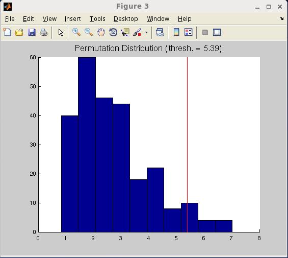
86 User s Documentation 86