User Documentation. BrainWave v User s Documentation -- Toronto, Canada

Transcription

1 User Documentation BrainWave v User s Documentation -- Toronto, Canada

2 Table of Contents Getting Started... 5 Introduction... 5 System Requirements... 5 Disclaimer & License... 6 Acknowledgements... 6 Helpful Tips to Keep in Mind Tutorial: The Basics... 8 Program Set-up... 8 Generating Beamformer Images Creating and Plotting Virtual Sensors Plotting Virtual Sensor Time Frequency Representations (TFRs) Importing Raw Datasets Group Analysis: General Group Analysis: Averages and Permutations Program Navigation (with screenshots) Main Menu Graphical User Interface (GUI) Main Menu: Single Dataset Section Main Menu: Beamformer Section Main Menu: Virtual Sensor Section Main Menu: Group Analysis Section User Documentation 2

3 Main Menu Drop-Down Options: Import Raw Data Main Menu Drop-Down Options: Average/Permutation GUI References.. 48 Appendix 1: Minimum-Variance Beamforming and SAM Calculations.. 49 Appendix 2: File Formats.. 55 Appendix 3: Calculation of MEG Forward Solution. 62 User Documentation 3

4 User Documentation 4

5 Getting Started Introduction BrainWave - Beamformer Reconstruction And INteractive WAveform Visualization Environment, is a user-friendly, special purpose, Matlab-based graphical user interface (GUI) for the computation of beamformer source images and waveforms from magnetoencephalography (MEG) data. It utilizes an integrated viewer for visualizing 4- dimensional image sequences, with simple point-and-click waveform and timefrequency plotting. BrainWave can also be used to perform MRI based spatial normalization and group analysis of source images using the SPM Matlab toolbox (installed separately). The documentation provided here will guide you through the basic features of this software package via program navigation screenshots as well as a brief tutorial on the basic set-up of your MEG data for analyses. BrainWave is not intended to be an extensive data editing or visualization toolbox for MEG data, nor does it attempt to replicate editing and data processing features that are already available in various MEG vendorʼs software, and assumes that users will use other processing tools to carry out artifact or bad channel removal or other pre-processing steps of their data. Rather than inventing yet another file format for MEG data, BrainWave uses the CTF MEG4 dataset (.ds) as its native format, and conversion utilities are provided to import MEG data from other MEG vendor formats by converting them to the.ds format. System Requirements The BrainWave toolbox currently runs on Linux (32 or 64 bit versions) and Mac OS X (version 10.6 or later recommended). A Windows version is not currently available but is planned for future release. Since BrainWave uses multi-threaded compiled C-mex User Documentation 5

6 functions and libraries for optimization, it is strongly recommended to run the toolbox on multiple core processors, with at least 2 GB of RAM. MATLAB Version 7.5 ( or higher is required. In order to utilize the spatial normalization and group analysis features, it is necessary to install the SPM Matlab toolbox. Although SPM2 and SPM5 should work, we highly recommend using the latest version of SPM8 ( For Macintosh platforms, 64-bit Matlab (e.g., Version 7.11 (R2010b)) or later is required for running SPM8. Although BrainWave works natively with the CTF-Omega system MEG data formats (e.g.,.ds and.mri), the CTF MEG4 software suite does not need to be installed to run BrainWave. Disclaimer & License This software package was developed by Dr. Douglas Cheyne and colleagues at the Toronto Hospital for Sick Children. This work is supported by operating grants from the Canadian Institutes of Health Research (MOP62479) and the Natural Sciences and Engineering Research Council of Canada (CPG104310). This program is provided free of charge without guarantees. It is to be used for RESEARCH PURPOSES ONLY, and has not been approved for clinical use. The distribution of this product is not permitted without permission by the developer and does not hold any warranty. Errors encountered using the program may be reported using our on-line mailing list or directly contacting at douglas.cheyne@utoronto.ca. To obtain a copy of the software, please visit for program download instructions. Acknowledgements The BrainWave interface and overall design was carried out by Natascha van Lieshout and Douglas Cheyne. Many other individuals have contributed to the BrainWave tooloox including, Sonya Bells, Andreea Bostan, Wilken Chau, Zhengkai Chen, Teresa Cheung, Paul Ferrari, Tony Herdman, Cecilia Jobst, Marc Lalancette, Brad Moores and Maher Quraan. Wavelet transformations algorithms are modified from Ole Jensenʼs 4D toolbox. The NIfTI file conversion routines were written by Jimmy Shen, ( Talairach conversion based on Talairach database available at Topoplot routines from the EEGLab package by Colin Humphries & Scott Makeig, CNL / Salk Institute, SPM - Welcome Trust Centre for NeuroImaging, Institute of Neurology, University College of London. User Documentation 6

7 Helpful Tips to Keep In Mind... **Always monitor the output of the MATLAB command window when processing data. It is here where you will find the details in what was done, and where any errors were encountered. **Keep your datasets organized. Weʼve included below, a tutorial on the suggested dataset organization for optimal BrainWave performance. User Documentation 7

8 Tutorial: The Basics Program Set-up Once you have downloaded the software ( the following steps must be taken to ensure proper performance of the BrainWave toolbox. Step 1: Unzip the downloaded file and save the folder to your computer. Step 2: Save the folder named bw_tools (and SPM8, if applicable) to your MATLAB path. Step 3: Format your dataset (*.ds) names. It is not mandatory, but extremely useful to name your datasets in the following manner, as BrainWave uses the filename structure to identify the subject associated with a given dataset in the following format: SubjectID_Condition_Name.ds where, SubjectID is the code or identifier for each of your subjects (these can be characters or numbers or a combination of both). The underscore delimits the end of the subjectid and is used by BrainWave to match this data automatically to a CTF MRI (.mri) file (see below). Anything that follows the underscore is up to you. Typically you would include the study and/or condition name here. Step 4: Prepare MRI and Head Model files (optional) For spatial (template) normalization and group analysis, currently a CTF formatted (.mri) MRI file is required (this will eventually be replaced with built-in User Documentation 8

9 routines to read native MRI data and perform co-registration independently of the CTF Software Suite). It is assumed that the head coil (fiducial) locations (coregistration) has been performed and saved in the.mri file. In addition, BrainWave has the capability to both manually specify a single-sphere head model (x, y and z origin), as well as multiple-sphere head models specified using the CTF headmodel (.hdm) file format, if available. Such files must be precomputed (e.g., using the CTF MRIViewer program) and saved in the dataset folder to be used. Step 5: Organize your data files. To help streamline group processing, the following data file organization is recommended. This will allow BrainWave to automatically find subjectʼs MRI files during spatial normalization. The first step is to save all dataset (.ds) files to a common folder. For example, letʼs call this folder Data. Your datasets file path should now looks something like this: Data / SubjectID_ConditionName.ds Within this same directory level, you will also need to create a folder containing your subjectʼs.mri file. It is again important to include the Subject ID before an underscore when naming this file, and include the name MRI in capitol letters. The file path for your.mri files should now look something like this: Data / SubjectID_MRI / SubjectID.mri If you use a different file organization and BrainWave has trouble finding your.mri file, it will prompt you to locate the file. However, this becomes tedious if you have many subjects and will interrupt automated processing of group data. NOTE: IMPORTANT NOTE ON CTF DATASETS: BrainWave assumes the use of multiple epoch (i.e., unaveraged) data to provide stable estimates of data covariance, but cannot distinguish between unaveraged and averaged CTF datasets as both have a.ds file extension. Averaged datasets created within the CTF software will contain up to two additional trials (the plus-minus and std. dev.) that must be removed if you want to apply the analysis to averaged data (although this approach is not generally recommended). User Documentation 9

10 Generating Beamformer Images The following tutorial will demonstrate how to create volumetric source images using BrainWave's minimum variance beamformer algorithm. Step 1: Launch Brainwave In the MATLAB command window, start BrainWave using the command: >> bw_start Step 2: Selecting a Dataset When the BrainWave Main Menu GUI pops up, the Matlab current working directory will already be selected as the Dataset Directory by default. To change this, select Set Dataset Directory in the Dataset section of the GUI. Select the directory that CONTAINS your datasets. Under the Data Directory list box select the dataset that you wish to use in this tutorial by clicking it. To the right of Set Dataset Directory button in the Dataset portion you should now see the name of the dataset as well as details about the dataset such as the number of trials, sample rate, and trial duration. All operations will be performed on this dataset until you select a different one by clicking on another dataset name. Step 3: Setting Data Parameters Hit the Data Parameters button in the Dataset section of the Main Menu GUI and select the data parameters you would like to use and hit the Save button. The parameters that you see when you first open the window are the default parameters, which they will be set back to if you hit the Set to Default button. Hitting the Cancel button will close the GUI and set the parameters back to whatever they were before you last opened the GUI. Once you save the parameters and close the dialog, the current parameters will be displayed in blue font in the Dataset section of the main GUI. The choice of data parameters is described in more detail the following sections. In most cases you will want to select a data bandpass, baseline setting, and head model before proceeding with source analysis. User Documentation 10

11 Step 4: Checking the Data Although BrainWave does may be used to detect activity that is not visible in the averaged sensor data, it is sometimes useful to view the averaged waveform data to confirm the presence of evoked responses, or detect the presence of any large artifacts. Select the View Data button in the bottom right corner of the Dataset section of the Main Menu GUI, to see the average of the data, for each channel (NOTE: the average is computed on the fly each time this window is opened using the current parameters settings.). Note that there is a special BrainWave drop down menu in the plot window. This will allow you to choose to see individual channels plotted, the global field power of the data or all the channels overplotted together. The map shows the topography at the cursor position, which can be manipulated with the mouse or arrow keys. As will be described below, the cursor position can also be used to conveniently specify the latency for generating a beamformer image. Step 5: Setting Image Options Click on the Image Options button in the Beamformer section of the Main Menu GUI. Select the parameters you would like to use in the generation of your beamformer images, noting that different options are unavailable depending on whether you have selected ERB or SAM type of beamformer to generate your images. Select Save to apply your changes. In most cases, the default options are a good starting point. Note that the parameters selected in Image Options only apply to the volumetric images and not virtual sensor calculations. If no Beamformer Options are selected, by default an optimized-orientation scalar beamformer is generated with rectified amplitudes at each voxel location. The mathematical details for beamformer computation are described in Appendix 1. Step 6: Choosing your Beamformer Select the kind of beamformer you would like to use by choosing between an Event-Related Beamformer (ERB) or the Synthetic Aperture Magnetometry or SAM beamformer (with pseudo-z, pseudo-t or pseudo-f options) using the radio buttons in the Beamformer section of the Main Menu GUI. Notice that depending on which method you select, different latency ranges and/or time window selections will become available. Note: All values of time User Documentation 11

12 are in seconds (s). Once you have selected your beamformer, you must fill in the appropriate latency information. If you have selected the ERB option, you must specify a start and end time range and step size. The step size is ignored if the start and end times are the same in which case only one image will be generated. As an optional shortcut, the Cursor Time button can be used to automatically set the ERB latency to the cursor latency in the most recently opened data plot window. If you select a SAM type beamformer you will need to specify the active time window (for pseudo-z images) in addition to the baseline time window (for pseudo-t and pseudo-f differential images). You can optionally select an active window step size and non-zero value for the number of steps. The latter will allow you to generate a sliding window sequence of SAM images, where the active window is shifted by the specified increment for each of N steps. If you do not wish to have BrainWave display the images and only create the files, uncheck the Display Images checkbox. If you have SPM2 or SPM8 installed a checkbox named Generate SPM images will become available to you should you wish to normalize the images and see them displayed in Talairach coordinates by the 4D Image Viewer. Step 7: Generate images Click on Generate Images in the Beamformer portion of the Main Menu GUI to start generating images. Again, detailed information regarding the progress of the calculations will be displayed in the MATLAB command window. Step 8: Viewing Data Once the beamformer image generation is complete, and provided you have the Display Images checkbox checked, the BrainWave 4D Image Viewer will appear displaying the images (in CTF coordinates for standard images, and Talairach coordinates for normalized SPM images). You can now use the bottom slider to move from one latency (or active window ) to the next. A threshold scale has also been provided to allow for manual image thresholding. To save an animation of all latencies Save as movie (.*avi or *.gif) options have been included in the File drop-down menu. Peak coordinates may be seen for each active window image by checking the Show peaks checkbox. In order to select User Documentation 12

13 custom coordinate locations (only available when viewing non-normalized images), double-click the desired image location. Your custom coordinates will appear under the coronal (top right) image. For added customization, you can also auto-scale the magnitude bar of each active window image by selecting the Autoscale checkbox option or show the negative values in each image, if available, by checking the *Plot negative checkbox. *NOTE: The Plot negative checkbox will only appear if there are negative valued voxels in the images to display. Only the use of Pseudo-T or Pseudo-Z beamformer options will produce such images. User Documentation 13

14 Creating and Plotting Virtual Sensors The following tutorial will demonstrate how to create a virtual sensor plot using the minimum variance beamformer algorithm. Step 1 - Step 4: Repeat same steps as described in the Generate Beamformer Images section to set your beamformer parameters, and to open a 4D Image Viewer window. This will allow you to interactively select voxels of interest to generate a virtual sensor. If you already know the coordinates of the voxel you wish to use, you still need to set the appropriate Data Parameters (filters settings, baseline, covariance window, etc.) as these will be used to generate the virtual sensor data each time. Step 5: Selecting the coordinates There are two ways of selecting the voxel coordinates you would like to create a virtual sensor plot with. You can enter them manually into the edit boxes under the Virtual Sensor section of the Main Menu or click on the Set to Peak Coords button next to the edit boxes if you have have previously opened the 4D Data Viewer and selected list peaks and clicked on one of the peaks in the list. Then select one of the Orientation radio buttons to indicate whether you would like the orientation used to be the optimized single direction (Scalar), the root-mean-square of both orthogonal directions (Vector), or Fixed (which if selected allows you to enter a unit vector specifying a fixed orientation. The flip button will multiply the orientation vector by -1 to flip the orientation of the current direction by 180 degrees). There is also an option to specify the location of the virtual sensor using Talairach coordinates. For instructions on how to use this option see note labeled VS Plots using Talairach Coordinates on page 35 in the Program Navigation chapter. Step 6: Set VS options (optional) Virtual sensors can be displayed in units of moment (nanoampere-meters) or pseudo-z. The latter is corrected for spatial distortions in the beamformer image using the pseudo-z scaling (i.e., are the same units as the volumetric images), whereas the former are in absolute units of source strength (dipole moment). User Documentation 14

15 The Set VS options dialog allows you to select the units of the virtual sensor data and plots by selecting the Moment or Pseudo-Z radio buttons. If you are using a scalar beamformer, a check box labeled Set polarity positive at latency and latency edit box will be enabled. Similar to the Flip button, this option allows you to force the polarity (flip the dipole orientation vector by 180 degrees) to have positive amplitude at a specified latency. This is often necessary when comparing virtual sensors in different brain locations or across subjects, as the scalar beamformer arbitrarily chooses the direction for the dipole source in the beamformer forward solution (e.g., the 100 ms component of an sensory evoked response may be arbitrarily set to be positive going in one hemisphere and negative going in the other hemisphere). Step 7: Generate the VS To create the virtual sensor, click on the Plot VS button in the left bottom corner of the Virtual Sensor section of the Main Menu GUI. Details about the progress of the calculations will be displayed in the MATLAB command window and the virtual sensor will be displayed in a separate plot window. Step 8: Viewing Data You will now see a plot of the virtual sensor data displayed in a standard Matlab plot window, with all the standard Matlab plotting features available to manipulate or save the plot. There is also a custom Brainwave pulldown menu that can be used to save the virtual sensor data in ASCII text files using Save VS average... Similarly, the Save VS single trial data... option can be used to save the raw (unaveraged virtual sensor data). The format of these files is described in Appendix 2. User Documentation 15

16 Plotting Virtual Sensor Time Frequency Representations (TFRs) The following tutorial will demonstrate how to create a time frequency representation plot of a virtual sensor, using the minimum variance beamformer algorithm. Step 1 - Step 6: *Repeat steps 1 through 6 as described in Creating and Plotting Virtual Sensors. Note that any VS polarity options will be ignored as the TFR is computed by integrating power over the individual trial VS data. Similarly, make sure you have not selected the Vector (RMS) option; otherwise, the time-frequency transformation will be applied to the rectified virtual sensor data with undesirable results such as frequency doubling. NOTE: The baseline specified in the Data Options will specify the baseline to be subtracted from the TFR amplitudes for each frequency bin. If no baseline is selected, the mean power across the entire epoch will be used instead. NOTE: Be sure to set a filter bandpass in the Data Parameters option dialog, as this will determine the frequency range of the TFR. Step 7: Setting TFR Options There are a number of options for the time-frequency plots that can be set using Set TFR Options... button at the bottom of the Virtual Sensor section of the Main Menu GUI. The default is a plot of virtual sensor power as a percent change from baseline. Other options are described in more detail in the next section. Step 8: Plot the TFR To create the TFR, click the Plot TFR button in the left bottom corner of the Virtual Sensor section of the Main Menu GUI. You will now see a plot of the data. Save TFR... and Load TFR... menu options in the BrainWave drop down menu in the figure window can be used to save or reload a previously computed TFR plot. User Documentation 16

17 Importing Raw Datasets The following tutorial will demonstrate how to create a CTF coordinate datasets from raw Yokogawa-KIT (*.con) or non-epoched (continuous) CTF datasets, into BrainWave friendly CTF coordinate datasets. Step 1: Select RAW datasets (Yokogawa, *.con files) In the Main Menu GUI, go to File -> Import Raw Data. The Import Data GUI will open. Go to File -> Open File, and select your raw dataset. Once selected, your Import Data GUI will fill in information from the dataset (i.e., Channels, Sample number, etc.) into the Input Parameters panel. The Sensor Layout panel includes the fiducial sensor coordinates (in centimeters), as well as the option to remove sensors from analysis by selecting the Channel Selector button (see next section). NOTE: Currently, BrainWave is only able to convert raw Yokogawa (*.con) files and continuous (ie. non-epoched) raw CTF datasets. Import modules for Elekta Neuromag datasets using the FIF interface are planned for future releases Step 2: Channel Selector (Optional) This optional channel selector GUI has been added should you decide to examine only specific sensor information (e.g., left hemisphere only). To do this, click the Channel Selector button. A GUI will display two columns of sensor names to include and exclude from the analysis. Default displays all sensors in the Include column. To exclude sensors (for example, sensor on the right hemisphere), simply select each sensor marked MRG*** and pressed the forward arrow which will place the selected channels into the Exclude column. Notice that the sensors selected will turn red and then grey when they are excluded. To reverse this process, simply re-select the channels would like to return to the Include column and press the back arrow. Click Apply to keep your settings. Step 3: Epoch Selection The selected dataset may now be epoched into CTF coordinates in one of two ways: The single epoch radio button may be selected to examine data at a User Documentation 17

18 specific time and/or duration. The second method is to utilize a Latency File (*.evt) which will mark the times at which an epoch marker will be placed. The latter method may be utilized by first selecting the Use Latency File radio button, and then the Load File button. A file window will appear, prompting you to select a latency file with the extension *.evt. Once selected, a list of all latencies (or epoch markers ) in this file will be displayed along with the total number of epoch times, which will be listed directly below the scrolling list. Select your epoch window times, and give a minimum separation value (NOTE: the minimum separation number must be a negative value). Step 4: Pre-Filter Data (Optional) The Pre-Filter Data option located in the bottom right panel, allows for the option to adjust bandpass filters (High Pass and Low Pass) prior to creating the dataset. NOTE: The Pre-Filter option will apply all filtering to segments of data that include samples that precede and follow the requested epoch length (by 50% of the total epoch length) to minimize filter transients. E.g., if you specify an epoch time from -1 to 2 seconds, a data segment from -1.5 to 2.5 second duration will be extracted from the raw data, filtered, then truncated to -1 to 2 seconds. Step 5: Save Average Dataset (Optional) This final option may be utilized to create an averaged dataset in addition to the newly converted CTF dataset. Unlike the standard CTF softwareʼs use of its averageds script, which displays three trials (average; plus-minus; standard deviation), BrainWave will create the average dataset only with the selection of the Save Average checkbox. Step 6: Create Dataset Press the Create Dataset button to initiate the conversion of your raw dataset into CTF coordinates based on the your customized selections. User Documentation 18

19 Group Analysis: General The following tutorial will demonstrate how to perform a simple group analysis. Step 1: Add Datasets to Group In the Main Menu GUI, simply select the desired datasets for group analyses from the dataset list in the Main Menu: Single Dataset Section, and click the Add to Group button located under this list. Notice that your selections will now appear within the Main Menu: Group Analysis section in the lower right hand region of the Main Menu GUI. Datasets may also be added to the group list by clicking the Add button in the Main Menu: Group Analysis Section. Notice that the datasets added in this manner will appear with a full path name to the desired dataset. Once your group list is complete, you may choose to save this group list (.list file) for later use. This is an especially important step should you wish to perform a permutation test (see Group Analysis: Average/Permutations section). The last method of adding datasets to the group list for analysis, is to load a pre-made.list file which lists a group of datasets. Should you need to delete any dataset from the group list, simply click the Delete button located beneath the group list. Step 2: Generate a Group Image The Generate Group Images button may now be selected once the image parameters have been set via the 1 Data Params button. By pressing the Generate Group Images button, a save window will appear where you must set the name for the group analysis images to be generated. Once complete, an averaged Talairach (.nii) image will be displayed. Within the directory, you will find three created files: (your_group_name).list, (your_group_name)wimage.list and (your_group name) wimage.nii. 1 Data Params settings are the same controls found in the Data Parameters window located in the Main Menu: Single Dataset Section. Therefore, if parameters have been set in the single dataset frame, those settings will remain when the group analysis Data Params GUI opens, and vise versa. User Documentation 19

20 IMPORTANT NOTE: Make sure that your listed datasets are in the Matlab path. Not doing this will result in the following Matlab error: Failed to find the dataset directory SubID_Condition.ds. See the Program Set-up tutorial for more information on how to avoid this error. WARNING: Please be aware that by selecting the checkbox labeled Plot individual images / waveforms, BrainWave will open the averaged CTF (.svl) image or the normalized (.nii) image for each subject, in addition to the group average image. For example, if you are analyzing 12 subjects, 13 figures windows will open. This warning also applies to the Plot Group VS and Plot Group TFR images to be described below. Step 3: Set-Up for Plot Group VS and Plot Group TFR In order to utilize the Plot Group VS and Plot Group TFR buttons in this frame, a Talairach position MUST first be selected. This is done by manually inputting Talairach coordinates in the Talairach radio button line within the Main Menu: Virtual Sensor Section. For example, you may choose to examine the peaks within the left premotor cortex by inputting the Talairach coordinates: X= -33; Y= -22; Z= 52. A way of finding this coordinate information can be done by selecting the Show Peaks in Talairach Coords (mm) checkbox in your spatially normalized (SPM) group (.nii) image (refer to the previous step on how to create this image). If your group image window was closed accidentally, or you wish to view the VS or TFR figures of previously created normalized images, simply go to File -> Image Viewer in you Main Menu GUI, and select your desired normalized NIfTI (.nii) image. NOTE: By default normalized images have the prefix w and the selection dialog filter selects only these files. If not, you may need to select All Files from the Files of Type drop down menu. Step 4: Plot Group VS Once the desired Talairach coordinate positions have been inputted, set your VS parameters by selecting the Set VS Options... button (see Virtual Sensor section for details on this optionʼs utilization) also located in the Virtual Sensor User Documentation 20

21 frame. A window will appear that allows you to set Talairach Options to find the highest peaks located around your set coordinate position, and within a specified duration window. We recommend that you set the Find closest peak within: option to start around 10mm and At a latency of: to around 50ms. If you find most subjects do not have peaks within this range (you will find this information in the Matlab command window), increase the peak search to 15mm, etc. Click OK. Now click Plot Group VS and name your VS image. Step 5: Plot Group TFR The first step here is to, again, check that you have inputted your desired Talairach coordinate, and select your Set TFR Options... parameters (see Time-Frequency section for a full description on what each option can be utilized). Click the Plot Group TFR button, and type in a name for your group TFR figure(s). (HINT: You may adjust the intensity of the colormap magnitudes by selecting Edit -> Colormap and adjusting the color data maximum and minimum values. NOTE: When plotting group virtual sensors or group TFRs, the individual image data is not automatically saved. However, a.vlist file is created that retains the CTF dataset name and corresponding CTF voxel coordinate used under the name you entered for the plot (e.g., cond1_ave.vlist). This information can be useful to recreate the virtual sensor plots without having to repeat the unwarping procedure or in custom applications, and will be incorporated in future analysis features for voxel-wise analyses. User Documentation 21

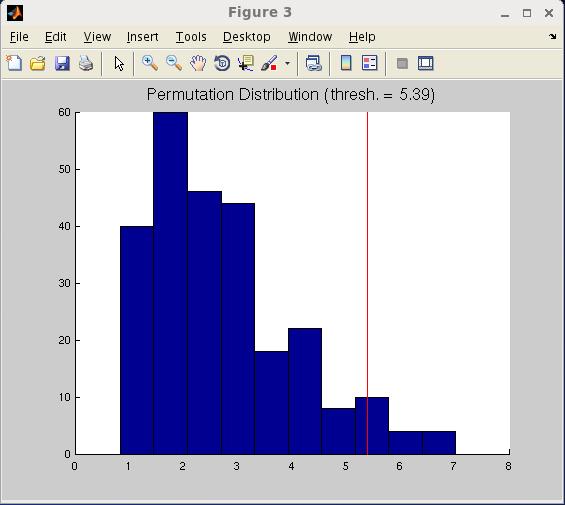
22 Group Analysis: Averages and Permutations The following tutorial will demonstrate how averages and permutations can be applied to groups. NOTE: The files analyzed here must be in.nii (Talairach or normalized) image files. Step 1: Open the Averaging/Permutations GUI In the Main Menu GUI, go to Tools -> Average/Permute Images to open the GUI. Step 2: Add Normalized (.nii) Images for Group Analysis There are two ways to add images for a group analysis. The first is to select your individual.nii (warped) files by selecting the Add File button and navigating to your selected datasets. The second method requires that a group.list file has been created (see Group Analysis tutorial section), and can therefore be selected from a directory by pressing the Read List button. Step 3: Set Options In the lower right hand frame (labeled Options), you may select the number of permutations 2 to be performed, and to what statistical significance (ie. alpha 3 ) you would like the data to be displayed in. To examine only certain parts of the brain during the permutation and averaging processes (for example, to eliminate large artifacts in some images that might bias the permutation distributions), you can select the Use ROI (MNI cords in mm) checkbox and set your coordinates to look in a particular region. For example, to only look at the results from the left hemisphere, simply change the values of X from (-75 to 70) to (-75 to 0), thus eliminating the right hemisphere data from the permutation test. 2 NOTE: The number of permutations cannot exceed the value of 2 N, where N = the number of subjects. The default is 2048 permutations, or less if the group contains fewer than 11 subjects. If desired a greater number of permutations can be selected up to the maximum, with a corresponding increase in computation time. 3 NOTE: The default alpha level is set to P < The smallest alpha level that can be selected is one bin size which = 1.0 / number of permutations. User Documentation 22

23 REMEMBER: Deselect the ROI option if you do not require it in all of your analyses. Step 4: Group Average (Optional) By pressing the Group Average button now, a normalized image file for the selected group will appear and will be identical to the group image generated from the Group Analysis frame in the Main Menu GUI. Step 5: Run Permutation and Average Analysis Pressing the Permute and Average button will prompt a save window which will again, require you to input a group name for this analysis. Two figures will display showing the permutation distribution plot and an averaged normalized image at a significance value of 0.05 (default alpha value). Notice that this value matches the vertical red line that appears in the title of the Permutations Distribution plot. Step 6: Create Contrast Image (Optional) Selecting the Create Contrast checkbox will open the Condition B section of the GUI window and allow you to add another group of images to be compared to Condition A. For example, Condition A may consist of a group of normalized images from one experimental condition, and Condition B may consist of the images from another condition. Note images will be contrasted depending on their order in the list i.e., each subjectʼs image must be in the SAME ORDER in each list for proper comparisons to be made. The resulting images created will be the average and/or permutations distributions figures depending on whether you selected the Average button or the Permute and Average button. In addition, you will notice that each subject compared to one another will have their own averaged.nii image labeled by subject order (e.g., subj_1_wimage,cw_-4_1.8,1-30hz_time=0.050-wimage,cw_-4_1.9984,1-30hz_time= nii). NOTE: Since this program is used to examine the peaks of activity within the brain, the images displayed would have shown peaks regardless of sign. To make it easier to decipher this difference, we've separated the comparisons into Condition A>Condition B and Condition B>Condition A. User Documentation 23

24 Program Navigation (with Screenshots) Main Menu Graphical User Interface (GUI) User Documentation 24

25 Main Menu: Single Dataset Section 1. Set Dataset Directory button: This button is used to select the directory that CONTAINS the dataset(s) that you would like to analyze (*see Program Set-Up section for details on how to set up your data for analysis using BrainWave). Do not click on a dataset (.ds) file within this directory, as this is itself a directory. 2. Add to Group button allows you to include a selected dataset into the group analysis list (see Group Analysis section). 3. Data Directory displays the currently selected dataset directory path. Click on a dataset in the file directory list below to select it for further analysis. 4. This area displays specific information about the currently selected dataset, including the number of sensors, number of trials, sampling rate and trial duration. 5. Refresh button updates the file directory list in case datasets within the directory location were added, moved or removed. 6. Data Parameters... button: Opens a GUI window (see figure below) that enables the setting of data parameters used for displaying and analysis. Note that any parameters changed here, must be saved in order for them to be utilized for analysis. User Documentation 25

26 Detailed description of dataset parameters are listed here: Bandpass: Sets the filter bandpass to be applied to data prior to display and computation of beamformers. This filter is applied prior to covariance calculation and generation of the beamformer images and virtual sensor data, using a non-phase shifting (bi-directional), 4 th order Butterworth filter. If enable is de-selected the bandpass of the saved dataset is used without any additional filtering. Covariance window: Sets the time range of data to be used when calculating the data covariance for the beamformer weights. By default the entire epoch is selected. A smaller window can be used to bias the beamformer weights to be sensitive to particular period within the data epoch. The Regularization factor is a constant noise power estimate (in femtotesla squared) that is applied to the diagonal of the covariance matrix prior to computing its inverse. This can be used in cases where the stability of the covariance inverse may be compromised (e.g., in cases of very few sample points or using averaged data). Baseline Correction: Sets the filter time range to use for baseline (offset) correction to be applied to data prior to calculating images or virtual sensors, including baseline correction of time-frequency plots. Head Model: Set the head model to be used for the magnetic field forward calculations. Use Sphere Origin allows you to specify the x, y and z coordinates of the origin of a single conducting sphere model. All coordinates in MEG head coordinates i.e., same coordinates as the sensor coils are defined in the dataset. Use Head Model allows you to specify a multiple overlapping sphere model saved in a CTF Head Model (.hdm) compatible format. (Format specified in Appendix 2). (Note: the Create.hdm file button is provided to allow you to create an.hdm file from a selected ASCII file containing digitized shape data. This will create a single and multisphere (.hdm) files in the same coordinates as in the file. (Format specified in Appendix 2) Beamformer Normalization: Sets the noise power estimate (in femtotesla per square root Hz) that is used to scale the noise normalized beamformer images and waveforms into units of pseudo-z. Only pseudo-z normalization is available at present. This value should be set to an estimate of MEG system noise. See Appendix 1 for details. User Documentation 26

27 NOTE: if epoch times differ between datasets, the program will automatically adjust these values when necessary to avoid out of range errors. You may need to check and occasionally change this by clicking the Set to Default button that will reset the range back to the entire epoch time of the current dataset. However, it is important to note that using the Set to Default button will also set everything else back to default (ex: head models set back to single sphere, etc.). NOTE: Baseline corrections will apply to both time plots and time frequency (TFR) plots. 7. Current Parameters (in blue font) will appear here once Data Parameters have been altered. 8. View Data button: Opens a figure displaying the averaged MEG sensor data (see top plot of figure below) and averaged field topography (lower right plot of figure below). Selecting the Show Sensors option will enable the sensor locations to be projected on the topographic virtual sensor. The arrow keys will move the time cursor (red vertical line) in the plot left and right one sample at a time, or the cursor can be moved by positioning the mouse cursor over the latency cursor and clicking and dragging. The drop down menu labeled BrainWave allows you to change the plot mode. User Documentation 27

28 Plot Global Field Power plots the RMS amplitude over all sensors as a single rectified waveform. The Plot Single Channel mode allows you to scroll through all channels one at a time. Furthermore, individual sensor channel activations can be seen in the Plot Single Channel view by simply clicking on the desired channel. User Documentation 28

29 Main Menu: Beamformer Section 9. The Event Related radio button enables event-related beamformer analysis to produce a sequence of source images at instantaneous latencies, via selection of latency values and step-size. By selecting a different start time and end time, a sequence of event-related images can be produced every step seconds. Set end time equal to the start time to generate a single latency image. All times are in units of seconds (s). If a data viewer window has been opened, the Cursor Time button can be used to automatically set the start and end time to the time of the latency cursor and map. 10. The SAM radio button allows for Synthetic Aperture Magnetometry differential beamformer analysis using the Pseudo-T or Pseudo-F metrics, as well as single state Pseudo-Z images of source power, although the latter is less frequency used. Selecting this option enables the time window selection options appropriate for the type of SAM image selected. Pseudo-T images involve subtracting the power in the baseline window from power in the active window, whereas Pseudo-F images involve taking the ratio of the power in the active and control windows. Computational formulae are given in Appendix 1. If a non-zero N number of steps is specified, the program will generate a sequence of N images by shifting the active window forward by Step Size seconds for each image (aka, sliding window SAM ). 11. Image Options... button opens a GUI (shown below), which allows you to select bounding box parameters, step size and various beamformer options. User Documentation 29

30 Detailed description of Image Option parameters are listed here: Bounding Box: This specifies the source reconstruction volume in the MEG head coordinate system (in cm). By convention the CTF coordinate system is assumed to have an origin mid-point between the ears, positive x-axis in direction of the nasion, and positive y-axis in direction of the left ear, and positive z-axis towards the top of the head. The default values should not need to be changed for head coordinates defined using these standard fiducial (head coil) placements (i.e., nasion and preauricular points). Voxel Step Size: This specifies the resolution of the reconstruction volume, or step size between nodes of the lattice 4. The default value of 5 mm should provide reasonable resolution with fast computation times, noting that computation time will increase by a factor of eight each time the resolution is doubled (E.g., a 2.5 mm resolution image will take 8 times longer to compute than a 5 mm image). A step size of less than 2 mm is not recommended for full brain volumes as out-of-memory errors will likely result. Beamformer options: By default the output metric of the beamformer is the amplitude (rectified to compensate for arbitrary polarity at any given voxel) at one time instant in the averaged data for event-related images, or the power integrated over time windows and trials for SAM at each voxel in the reconstruction volume, using the optimized current orientation determined at each grid point. In BrainWave this is termed a scalar beamformer. If the vector beamformer option is selected, then two orthogonal current directions at each grid point are used to compute the spatial filter output, and the root-mean-square magnitude from both directions is used instead. For event-related images, three additional options can be chosen: The option compute mean ERB over range computes images at all latencies in a chosen range as it would normally do, but generates a single image that is the mean value averaged across all latencies at each voxel. An additional two options are for specialized use, for example, where the user may want to generate noise images for statistical testing. The option Compute Plus/Minus ERB creates an image by 4 Note that for beamformer images the source activity is computed independently at discrete points on a 3 dimensional reconstruction lattice or grid, although the term voxel or voxel location is often used for convenience. However, the voxels in beamformer images have no real dimensions as for example, in the case of MRI volumes. User Documentation 30

31 applying the beamformer weights to the plus-minus (or anti-average ) to remove the power of any time-locked evoked response from the image. The option compute non-rectified ERB turns off the rectification of amplitude at each voxel to produce an image with positive and negative values where noise should be distributed about zero. Further details of the meaning of various parameters in the calculation of the beamformer images can be found in Appendix Display Images check box can be unselected should you wish to generate the output files only without displaying plotted figures. 13. Generate SPM Images check box option tells BrainWave to also generate a spatially normalized (SPM template space) source image when Generate Images is selected. This will require a co-registered.mri file for each subject. NOTE on SPM Normalization: The first time this option is used for any subject, BrainWave will be required to carry out a number of steps prior to generating the normalized source images. First, it will search for the subjectʼs.mri file and extract the anatomical 3-dimensional volume from the MRI corresponding to the source reconstruction volume (Bounding Box) and save this image in the <SubjectID_MRI> directory in NIfTI format (or Analyze format if SPM2 is used) with an identifiable name (e.g., SubjectID_resl_-10_10_-8_8_0_14.nii). SPM will then be invoked to compute linear and non-linear warping parameters that will warp functional volumes corresponding to this bounding box to standardized (MNI) space using the SPM T1 template. This process may take a few minutes and will open additional SPM output windows to monitor progress that will also display the match between the subjects and template MRI, which provides a good visual check that the process ran correctly. This process generates the file <SubjectID_resl_-10_10_-8_8_0_14_sn3d.mat> that is subsequently used to spatially normalize the beamformer source images computed in this volume. Note: the SubjectID_resl_-10_10_-8_8_0_14_sn3d.mat file is slightly modified by BrainWave to save the MEG bounding box values to be able to unwarp from normalized space back to MEG coordinates.) This is necessary to be able to generate virtual sensors using Talairach coordinates, described below. These SPM files only have to be generated once per subject so that SPM routines will not be called again, unless these files are deleted, or the beamformer bounding box is changed. User Documentation 31

32 NOTE: Generate SPM Images option will work only if you have installed the SPM software toolbox and added it to your Matlab path. Please see System Requirements section for download options. 14. Generate Images button (without Generate SPM Images option) generates the requested images (which are saved as.svl files) and displays the source image in an Image Viewer window. The Image Viewer displays a single image, or sequence of images as a Maximum Intensity Projection (MIP) plot in all cardinal directions which shows the location and intensity distribution of source power throughout the brain in one glance (sometimes referred to as a glass-brain plot). Note on image files: All beamformer source images are first computed in MEG coordinate space and written to disk files in the CTF SAM volume (.svl) file format, rather than being held in memory to avoid memory limitations. These files can be found in the ANALYSIS directory located within each dataset (.ds) directory and can be viewed by opening a new viewer window (this can be done by either selecting Image Viewer the Main Menu File Menu or New Viewer in an open viewer window) and selecting an.svl file. These files are labeled with identifiable names containing the filter settings and image latency. If sequences of images are created, an ASCII list file (.list) containing the files names of all images files is also created and this can be used to read back in the entire sequence of images into an Image Viewer. When normalized SPM8 images or image sequences are created, they are saved in NIfTI format with the same file names as the.svl image files prepended with the w (for warped ) at the beginning of the filename, with corresponding list files. Further details of file formats used by BrainWave are given in Appendix 2. The Image Viewer interface will appear slightly different depending on whether you are displaying images in native (CTF) coordinates (*.svl file) or in normalized (SPM) coordinates (w*.nii file) (see an example of both CTF and SPM images following this section). Common viewing features including: A slider tool has been made available to allow you to manually adjust the image Threshold. This is set at an arbitrary value of 40% of the maximum when first opening an image. The Overall Maximum value can also be changed to adjust the overall scale this is useful to see weaker peaks in the presence of a larger peak at a different latency. User Documentation 32

33 An Autoscale option that scales each image in a sequence to its own maximum value, otherwise, images will be scaled to the global maximum value in the entire sequence. A Plot negative option that if selected will display any negative values in the image file. This will be disabled if the image has all positive values as in the case of ERB images and only applies to differential images or contrasts. The main difference between displaying CTF and SPM source images is in the behaviour of the Show Peaks feature of Image Viewer. Selecting the Show Peaks option displays a list of CTF coordinates for peaks identified in the image. Peaks are defined by using a peak finding algorithm, similar to that in the CTF MRIViewer application. Note that the number of peaks found depends on the current threshold. Caution should be used when changing the threshold value when Show Peaks is selected, as setting it too low will result in the peak finding algorithm finding many spurious peaks and can even cause MATLAB to temporarily hang. Doubleclicking a peak of interest in the list box moves the blue cross-hair cursor to move to that location and makes this the current selected peak for virtual sensor plotting (described below). The coordinates of this new location are listed underneath the coronal view (top right) image. Double-clicking on the MIP views will also move the cross-hair cursor to that location and display the coordinates below the coronal view (top right). If the Generate SPM Images checkbox option is selected, a second Image Viewer window will appear displaying the SPM images in addition to the CTF image (.svl). In this case, the Show Peaks option displays a detailed list of peak activity as before, but with the option of viewing them in native MNI coordinates (these are the actual image coordinates, as Talairach 3 coordinates (default option), or even as CTF coordinates). In the latter case, the CTF coordinates are determined by unwarpin the MNI to CTF space as described earlier. When viewing in Talairach coordinates, the anatomical brain region or gyrus and Broadmann Area (BA) labels corresponding to the peak are listed next to the coordinates, using the Talairach atlas database ( BA labels are only listed if a voxel containing gray matter is located within 5mm of the peak in the database. Notice that the custom coordinates option (blue cross-hair selection) is not available in this view. 3 Conversion from MNI to Talairach coordinates is done using the mni2tal and tal2mni scripts available at: User Documentation 33

34 Example: 4D Image Viewer in CTF coordinates (.svl) Example: 4D Image Viewer in Talairach (normalized) coordinates (.nii) User Documentation 34

35 Main Menu: Virtual Sensor Section 15. Voxel (MEG) The coordinates for generating a virtual sensor average or timefrequency plot may be entered here manually, or can be set to a peak location automatically by first selecting a peak in the Show Peaks list in any currently open Image Viewer and then clicking on the Set to Peak Coords button. Voxel (Talairach) option allows one to specify Talairach coordinates instead of MEG coordinates for the virtual sensor. This calculation will take longer due to the need to determine the unwarping parameters and optionally the search radius for finding the true peak (see VS Options). NOTE: VS plots using Talairach coordinates: In order to generate and plot virtual sensor waveforms from Talairach coordinates, BrainWave must determine the unwarping parameters from SPM space to MEG (CTF) coordinate space. When selecting this option, the program will first compute the normalized image using the current data and image parameters to obtain these parameters. This will include the need to compute the warping parameters using SPM and this subjectʼs.mri file, if this has not already been done. This will allow the program to determine the location of that Talairach coordinate in MEG coordinates for that subject. In certain cases, the unwarping procedure may be used to find the location of a corresponding peak in an individualʼs source image, for example, if using the group averaged Talairach location. However, due to spatial distortions due to the warping procedure, the unwarped peak coordinates may close to, but not exactly in the same location as the true peak location in the image, and this can result in significant attenuation of the virtual sensor amplitude. In order to compensate for this, an option is provided to have BrainWave find the true peak within some distance of the unwarped coordinates, using a search radius specified in VS Options. In this case, it is extremely important to ensure that the appropriate latency (for ERB images) or time windows (for SAM images) are selected. Note, that details of this process and search algorithm results will be printed to the Matlab command window and should be monitored closely to ensure that the correct peaks are being selected! 16. Orientation: As in the case of the beamformer Image Options, different methods can be used to determine how the current orientation for the forward solution at each voxel is defined. These can be set to Scalar or Vector (RMS), User Documentation 35

36 and in the case of virtual sensors a third option of Fixed orientation, which allows the current direction to be independently fixed to a given direction vector which can be entered into the text edit boxes (this is assumed to be a unit length vector but will be adjusted automatically). When Scalar option is chose, the computed orientation will be displayed next to the radio button afterwards, and for convenience, the coordinates displayed in the Fixed text edit boxes. The Flip button allows the flipping of the orientation vector polarity by 180 degrees (i.e., to flip the polarity of the virtual sensor). Note that if the Vector option is chosen the plots will show the rectified waveforms computed as the root-mean-squared amplitude in multiple current directions. Refer to Appendix 1 for calculation details. 17. Virtual Sensor (VS) options may be set using the Set VS Options button (see image below), where your choice of y-axis units (Moment or Pseudo-Z) may be selected, as well as an option to set the polarity of the virtual sensor to be positive at a desired latency. If Talairach coordinates have been selected, the option will be enabled to set the Search Radius for finding peak source activity from unwarped locations (see notes above). A search radius of 10 to 15 mm is recommended. Larger values may select the incorrect peak in another brain region, and too small of a search radius will fail to find the true peak and the search algorithm will default to the original start location. The text box below allows a latency to be defined to generate the source image to be searched. Note that the search radius only applies to ERB images and for differential images the currently defined time windows will be used instead. User Documentation 36

37 Plot VS button then plots the averaged virtual sensor amplitude over time (see figure below). A custom BrainWave drop-down menu allows for the option to save the VS data values (averaged or raw data) in an ASCII file using the Save VS Average and/or Save VS single trial data. The formats for these files are described in Appendix In addition to plotting the averaged virtual sensor the Plot TFR button can be used to plot a time frequency representation (TFR) of the virtual sensor data using a Morlet wavelet transformation of the power in the raw (single trial) virtual sensor data. Several options for the TFR plots may be set using the Set TFR Options...(see figure below): User Documentation 37

38 Detailed description of TFR Option parameters are listed here: Freq. Bin Size: Specifies the frequency bin size for the wavelet transformation in Hz. Default is 1 Hz bins. Morlet Width: Specifies the number of cycles used to generate the Morlet wavelets. Lower numbers will provide more temporal resolution with a trade-off in frequency resolution. Default is 7 cycles. Zero endpoints: Can be used to zero values at the beginning and end of the TFR plots to minimize the appearance of end effects. Default is 3% of the trial duration. Subtract mean: This options removes the mean VS from the single trial data prior to computing the frequency transformation. This can be used to remove energy of phase-locked (i.e., evoked response) components in the data to plot only the induced power. Plot Mode: Scaling options for the TFR plots include Plot power: plot the raw TFR power as function of baseline. Plot Percent Change plots TFR power as a percent change from the baseline*. This provides better normalization of intensity changes across frequencies. Plot Z scores. Plots TFR as deviations in units of standard deviation (z-scores) from the baseline. Phase-locking Factor: Plots the phase-locking factor (also known as inter-trial coherence) which is a metric from 0 to 1, where 1 = complete phase-locking across trials within a given frequency bin. User Documentation 38

39 *NOTE: For all TFR plots, the values are adjusted by subtracting the mean power within each frequency bin. If no baseline window is defined in the Data Parameters GUI, then the mean of the entire trial is subtracted. Plot TFR button then plots a time-frequency figure (see example figure below) which can be saved as a.mat file under the BrainWave drop-down menu called Save TFR data. User Documentation 39

40 Main Menu: Group Analysis Section 19. The Main Menu: Group Analysis Section ultimately creates an average Normalized image among the selected group of datasets. As mentioned in the Group Analysis tutorial, there are a couple of ways to select datasets for group analysis. The first is to select the datasets individually from the Main Menu: Single Dataset Section and click the Add to Group button. The second method is to press the Add button and manually navigate to each dataset. This method will display the entire path of the selected dataset. To delete and datasets, select the dataset and press the Delete button. The Save List button simply saves the selected group of datasets to a file that can be loaded at a later time by pressing the Load List button. 20. Data Params button opens a GUI that is identical to the Data Parameters button in the Main Menu: Single Dataset Section. Settings saved in either GUI will be carried over to the other, so be sure to make the necessary changes if applicable. The Generate Group Images button will then generate an averaged Talairach image of the selected datasets (see figure 4D Image Viewer in Talairach (normalized) coordinates (.nii) under number 14 in the Main Menu: Single Dataset Section above for an example image). 21. The Plot Group VS and Plot Group TFR plot both averaged group virtual sensor and time-frequency representation figures, respectively. Details on how to use either option have been added to the Group Analysis Tutorial section. 22. When the Plot Individual images / waveforms checkbox has been selected, all the averaged images (CTF (.svl) and Talairach'd (.nii) images if Generate Group Images was selected for example) for each subject will open, in addition to the group averaged Talairach'd image. For example, if you are analyzing 12 subjects, 25 figures windows will open. This warning also applies to the Plot Group VS and Plot Group TFR images buttons. User Documentation 40

41 Main Menu Drop-Down Option: Import Raw Data GUI Detailed description of Import Raw Data GUI parameters are listed here: Input Parameters: Specifies the information of the selected raw dataset. Currently, the datasets must be in Yokogawa (*.con) or continuous CTF dataset format. Sensor Layout: Specifies the x, y and z location of right ear, left ear and nasion fiducials. These values cannot be changed. The Channel Selector button opens a GUI that allows for the selection and/or removal of specific MEG channels from analyses. Currently, the Channel Selector button works only for Yokogawa datasets. The following images show an example of the Channel Selector GUI and how it works. User Documentation 41

42 By default, all channels are located in the Include column. To select a channel, simply click on the desired channel name and notice the sensor light up in red on the MEG helmet graphic. You may also select multiple channels, as seen in the figure below: Pressing the Forward arrow button removes the selected channels from the Include column and places them in the Exclude column, as seen in the figure below. Notice that these sensors turn grey when excluded: User Documentation 42

43 Similarly, by selecting the channels you want to include in your analyses, simply select the channels from the Exclude column and press the Back arrow button. Click Apply to save your changes. Epoch Selection: The Single Epoch radio button allows for you to produce a dataset that only looks at a specific time window (in seconds), while the Use Latency file radio button provides BrainWave with a text file of latency values (an.evt file that is to be navigated to after pressing the Load File button) that is used to epoch the continuous raw dataset. The latency values are then automatically listed within the Selected Latencies: scroll box, and can then be epoched based on customized parameters using the Epoch Window: options. By providing Start, End and Minimum Separation 5 values (each are in seconds, s), you will notice that the total number of epochs (displayed under the Selected Latencies: scroll box) will change as you make adjustments; excluding those trials that do not fit the desired epoch specifications. Options: In this frame, the option to pre-filter the dataset with High Pass and Low Pass bandpass values, as well as saving an averaged dataset is available here. NOTE: Errors may occur with High Passvalues around 0.1. The High Pass value set to 0.3 as the lowest value seems to work well. NOTE: The averaged 5 The Minimum Separation value must to be inputted as a negative number (e.g., -0.3 seconds). User Documentation 43

44 dataset generated is not the same as that produced by CTFʼs averageds script which produces three trials containing the average, plus-minus and standard deviation. BrainWave instead only produces an average dataset (or, the first trial to the CTF script). User Documentation 44

45 Main Menu Drop-Down Option: Average/Permutation GUI Detailed description of Average/Permutations GUI are listed here: Read List: Opens a previously created list (*.list file) of a group of images to be analyzed. Please see the Main Menu: Group Analysis Section tutorial for details on how to generated this list. Add File: This button allows you to select and add other.nii subject files to the list for averaging and/or permutation analyses. Clear List: Simply clears the selected list of subjects from being analyzed. NOTE: this option clears the ENTIRE list when selected. Create Contrast Image: By selecting this checkbox, positive (Condition A > Condition B) and negative (Condition B > Condition A) comparisons may be made. Plot Individual Images: This checkbox option will display all individual averaged Talairach (.nii) images for each subject in addition to the group averaged Talairach image and/or permutation distribution figure. Alpha: The statistical significance threshold (alpha) may be adjusted. The default is currently set to a P-value of User Documentation 45

46 No. of Permutations: The number shown in this box is the highest possible combination of permutations that can be performed on the selected group of datasets. Use ROI (MNI coords in mm): The default region of interest (ROI) values (currently in MNI coordinates) have been set to include the entire brain, but can easily be adjusted to restrict the analysis region to a specific region of interest. For example, to analyze the left hemisphere only for all subjects, simply change the X- values from the default (-75 to +75) to (-75 to 0). Average: This button generates an averaged Talairach image of the selected group list images. NOTE: This generated image is virtually the same as the group averaged Talairach image created in the Main Menu: Group Average Section tutorial. Permute and Average: This button generates an averaged Talairach group image with only regions of within the significance level displayed, as well as a permutation distribution figure (see example average and permutation distribution images below). NOTE: The significance threshold value automatically set on the averaged.nii image will match the value shown in the permutation distribution figure title. User Documentation 46

47 User Documentation 47

48 References Event-related beamformer images and virtual sensor calculations are based on algorithms described in: Cheyne D., Bakhtazad L. and Gaetz W. (2006) Human Brain Mapping 27: Cheyne D., Bostan AC., Gaetz W, Pang EW. (2007) Clinical Neurophysiology, Vol 118 pp Differential images and pseudo-z normalization based on the SAM algorithm described in: Robinson, S. and Vrba J. (1999). Functional neuroimaging by synthetic aperture magnetometry. Nenonen J, Ilmoniemi RJ, Katila T, editors. Biomag p Forward solutions are based on spherical conductor dipole model: Sarvas, J., Basic mathematical and electromagnetic concepts of the biomagnetic inverse problem. Phys Med Biol, 32; 11-22, User Documentation 48