Lecture 1 Introduction & Fundamentals

Transcription

1 Digital Image Processing Lecture 1 Introduction & Fundamentals Presented By: Diwakar Yagyasen Sr. Lecturer CS&E, BBDNITM, Lucknow

2 What is an image? a representation, likeness, or imitation of an object or thing a vivid or graphic description something introduced to represent something else 2

3 DIGITAL IMAGE 3

4 DIGITAL IMAGE 4

5 FROM ANALOG TO DIGITAL Imaging systems Sample and quantize Digital storage (disk) Digital computer On-line buffer Display output object observe digitize store process Refresh /store Record 5

6 Sampling 256x256 64x64 6

7 Quantisation 8 bits

8 Quantisation cont. 256x levels 256x levels 8

9 Quantisation cont. 256x levels 256x256 2 levels 9

10 Coloured Image 10

11 Intensity (Gray-Level) Image 11

12 Binary Image 12

13 Image Processing manipulation of multidimensional signals image (photo) video CT, MRI f ( x, y) f ( x, y, t) f ( x, y, z, t) 13

14 What is Digital Image Processing? Digital Image a two-dimensional function x and y are spatial coordinates The amplitude of f is called intensity or gray level at the f ( x, y) point (x, y) Digital Image Processing process digital images by means of computer, it covers low-, mid-, and high-level processes low-level: inputs and outputs are images mid-level: outputs are attributes extracted from input images high-level: an ensemble of recognition of individual objects Pixel the elements of a digital image 14

15 Origins of Digital Image Processing Sent by submarine cable between London and New York, the transportation time was reduced to less than three hours from more than a week 15

16 Origins of Digital Image Processing 16

17 Sources for Images Electromagnetic (EM) energy spectrum Acoustic Ultrasonic Electronic Synthetic images produced by computer 17

18 Electromagnetic (EM) energy spectrum Major uses Gamma-ray imaging: nuclear medicine and astronomical observations X-rays: medical diagnostics, industry, and astronomy, etc. Ultraviolet: lithography, industrial inspection, microscopy, lasers, biological imaging, and astronomical observations Visible and infrared bands: light microscopy, astronomy, remote sensing, industry, and law enforcement Microwave band: radar Radio band: medicine (such as MRI) and astronomy 18

19 Examples: Gama-Ray Imaging 19

20 Examples: X-Ray Imaging 20

21 Examples: Ultraviolet Imaging 21

22 Examples: Light Microscopy Imaging 22

23 Examples: Visual and Infrared Imaging 23

24 Examples: Visual and Infrared Imaging 24

25 Examples: Infrared Satellite Imaging USA

26 Examples: Infrared Satellite Imaging 26

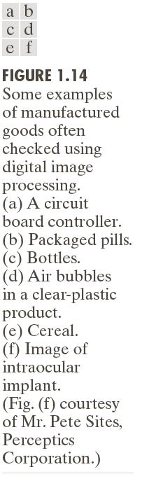
27 Examples: Automated Visual Inspection 27

28 Examples: Automated Visual Inspection Results of automated reading of the plate content by the system The area in which the imaging system detected the plate 28

29 Example of Radar Image 29

30 Satellite image Volcano Kamchatka Peninsula, Russia 30

31 Satellite image Volcano in Alaska 31

32 Medical Images: MRI of normal brain 32

33 Medical Images: X-ray knee 33

34 Medical Images: Ultrasound Five-month Foetus (lungs, liver and bowel) 34

35 Astronomical images 35

36 Examples: MRI (Radio Band) 36

37 Examples: Ultrasound Imaging 37

38 Fundamental Steps in DIP Extracting image components Improving the appearance Result is more suitable than the original Partition an image into its constituent parts or objects Represent image for computer processing 38

39 Light and EM Spectrum c E h, h: Planck's constant. 39

40 Light and EM Spectrum The colors that humans perceive in an object are determined by the nature of the light reflected from the object. e.g. green objects reflect light with wavelengths primarily in the 500 to 570 nm range while absorbing most of the energy at other wavelength 40

41 Light and EM Spectrum Monochromatic light: void of color Intensity is the only attribute, from black to white Monochromatic images are referred to as gray-scale images Chromatic light bands: 0.43 to 0.79 um The quality of a chromatic light source: Radiance: total amount of energy Luminance (lm): the amount of energy an observer perceives from a light source Brightness: a subjective descriptor of light perception that is impossible to measure. It embodies the achromatic notion of intensity and one of the key factors in describing color sensation. 41

42 Digital Image Fundamentals HUMAN Vision 42

43 Image Acquisition Transform illumination energy into digital images 43

44 Image Acquisition Using a Single Sensor 44

45 Image Acquisition Using Sensor Strips 45

46 Image Acquisition Process 46

47 A Simple Image Formation Model f ( x, y) i( x, y) r( x, y) f ( x, y) : intensity at the point ( x, y) i( x, y) : illumination at the point ( x, y) (the amount of source illumination incident on the scene) r( x, y) : reflectance/transmissivity at the point ( xy, ) (the amount of illumination reflected/transmitted by the object) where 0 < i( x, y) < and 0 < r( x, y) < 1 47

48 Some Typical Ranges of illumination Illumination Lumen A unit of light flow or luminous flux Lumen per square meter (lm/m 2 ) The metric unit of measure for illuminance of a surface On a clear day, the sun may produce in excess of 90,000 lm/m 2 of illumination on the surface of the Earth On a cloudy day, the sun may produce less than 10,000 lm/m 2 of illumination on the surface of the Earth On a clear evening, the moon yields about 0.1 lm/m 2 of illumination The typical illumination level in a commercial office is about 1000 lm/m 2 48

49 Some Typical Ranges of Reflectance Reflectance 0.01 for black velvet 0.65 for stainless steel 0.80 for flat-white wall paint 0.90 for silver-plated metal 0.93 for snow 49

50 Image Sampling and Quantization Digitizing the coordinate values Digitizing the amplitude values 50

51 Image Sampling and Quantization 51

52 Representing Digital Images 52

53 Representing Digital Images The representation of an M N numerical array as f ( x, y) f (0,0) f (0,1)... f (0, N 1) f (1,0) f (1,1)... f (1, N 1) f ( M 1,0) f ( M 1,1)... f ( M 1, N 1) 53

54 Representing Digital Images The representation of an M N numerical array in MATLAB f ( x, y) f (1,1) f (1,2)... f (1, N) f (2,1) f (2,2)... f (2, N) f ( M,1) f ( M,2)... f ( M, N) 54

55 Representing Digital Images Discrete intensity interval [0, L-1], L=2 k The number b of bits required to store a M N digitized image b = M N k 55

56 Representing Digital Images 56

57 Spatial and Intensity Resolution Spatial resolution A measure of the smallest discernible detail in an image stated with line pairs per unit distance, dots (pixels) per unit distance, dots per inch (dpi) Intensity resolution The smallest discernible change in intensity level stated with 8 bits, 12 bits, 16 bits, etc. 57

58 Spatial and Intensity Resolution 58

59 Spatial and Intensity Resolution 59

60 Spatial and Intensity Resolution 60

61 Image Interpolation Interpolation Process of using known data to estimate unknown values e.g., zooming, shrinking, rotating, and geometric correction Interpolation (sometimes called resampling) an imaging method to increase (or decrease) the number of pixels in a digital image. Some digital cameras use interpolation to produce a larger image than the sensor captured or to create digital zoom 61

62 Image Interpolation: Nearest Neighbor Interpolation f 1 (x 2,y 2 ) = f(round(x 2 ), round(y 2 )) =f(x 1,y 1 ) f(x 1,y 1 ) f 1 (x 3,y 3 ) = f(round(x 3 ), round(y 3 )) =f(x 1,y 1 ) 62

63 Image Interpolation: Bilinear Interpolation (x,y) f (, ) 2 x y (1 a) (1 b) f ( l, k) a (1 b) f ( l 1, k) (1 a) b f ( l, k 1) a b f ( l 1, k 1) l floor( x), k floor( y), a x l, b y k. 63

64 3 Image Interpolation: Bicubic Interpolation The intensity value assigned to point (x,y) is obtained by the following equation 3 3 f ( x, y) a x y i0 j0 The sixteen coefficients are determined by using the sixteen nearest neighbors. ij i j 64

65 Examples: Interpolation 65

66 Examples: Interpolation 66

67 Examples: Interpolation 67

68 Examples: Interpolation 68

69 Examples: Interpolation 69

70 Examples: Interpolation 70

71 Examples: Interpolation 71

72 Examples: Interpolation 72

73 Basic Relationships Between Pixels Neighborhood Adjacency Connectivity Paths Regions and boundaries 73

74 Basic Relationships Between Pixels Neighbors of a pixel p at coordinates (x,y) 4-neighbors of p, denoted by N 4 (p): (x-1, y), (x+1, y), (x,y-1), and (x, y+1). 4 diagonal neighbors of p, denoted by N D (p): (x-1, y-1), (x+1, y+1), (x+1,y-1), and (x-1, y+1). 8 neighbors of p, denoted N 8 (p) N 8 (p) = N 4 (p) U N D (p) 74

75 Basic Relationships Between Pixels Adjacency Let V be the set of intensity values 4-adjacency: Two pixels p and q with values from V are 4-adjacent if q is in the set N 4 (p). 8-adjacency: Two pixels p and q with values from V are 8-adjacent if q is in the set N 8 (p). 75

76 Basic Relationships Between Pixels Adjacency Let V be the set of intensity values m-adjacency: Two pixels p and q with values from V are m-adjacent if (i) q is in the set N 4 (p), or (ii) q is in the set N D (p) and the set N 4 (p) N 4 (p) has no pixels whose values are from V. 76

77 Basic Relationships Between Pixels Path A (digital) path (or curve) from pixel p with coordinates (x 0, y 0 ) to pixel q with coordinates (x n, y n ) is a sequence of distinct pixels with coordinates (x 0, y 0 ), (x 1, y 1 ),, (x n, y n ) Where (x i, y i ) and (x i-1, y i-1 ) are adjacent for 1 i n. Here n is the length of the path. If (x 0, y 0 ) = (x n, y n ), the path is closed path. We can define 4-, 8-, and m-paths based on the type of adjacency used. 77

78 Examples: Adjacency and Path V = {1, 2}

79 Examples: Adjacency and Path V = {1, 2} adjacent 79

80 Examples: Adjacency and Path V = {1, 2} adjacent m-adjacent 80

81 Examples: Adjacency and Path V = {1, 2} 01,1 11,2 11, ,1 22,2 02, ,1 03,2 13, adjacent m-adjacent The 8-path from (1,3) to (3,3): (i) (1,3), (1,2), (2,2), (3,3) (ii) (1,3), (2,2), (3,3) The m-path from (1,3) to (3,3): (1,3), (1,2), (2,2), (3,3) 81

82 Basic Relationships Between Pixels Connected in S Let S represent a subset of pixels in an image. Two pixels p with coordinates (x 0, y 0 ) and q with coordinates (x n, y n ) are said to be connected in S if there exists a path (x 0, y 0 ), (x 1, y 1 ),, (x n, y n ) Where i,0 i n,( x, y ) S i i 82

83 Basic Relationships Between Pixels Let S represent a subset of pixels in an image For every pixel p in S, the set of pixels in S that are connected to p is called a connected component of S. If S has only one connected component, then S is called Connected Set. We call R a region of the image if R is a connected set Two regions, R i and R j are said to be adjacent if their union forms a connected set. Regions that are not to be adjacent are said to be disjoint. 83

84 Basic Relationships Between Pixels Boundary (or border) The boundary of the region R is the set of pixels in the region that have one or more neighbors that are not in R. If R happens to be an entire image, then its boundary is defined as the set of pixels in the first and last rows and columns of the image. Foreground and background An image contains K disjoint regions, R k, k = 1, 2,, K. Let R u denote the union of all the K regions, and let (R u ) c denote its complement. All the points in R u is called foreground; All the points in (R u ) c is called background. 84

85 Question 1 In the following arrangement of pixels, are the two regions (of 1s) adjacent? (if 8-adjacency is used) Region 1 Region 2 85

86 Question 2 In the following arrangement of pixels, are the two parts (of 1s) adjacent? (if 4-adjacency is used) Part 1 Part 2 86

87 In the following arrangement of pixels, the two regions (of 1s) are disjoint (if 4-adjacency is used) Region 1 Region 2 87

88 In the following arrangement of pixels, the two regions (of 1s) are disjoint (if 4-adjacency is used) foreground background 88

89 Question 3 In the following arrangement of pixels, the circled point is part of the boundary of the 1-valued pixels if 8-adjacency is used, true or false?

90 Question 4 In the following arrangement of pixels, the circled point is part of the boundary of the 1-valued pixels if 4-adjacency is used, true or false?

91 Distance Measures Given pixels p, q and z with coordinates (x, y), (s, t), (u, v) respectively, the distance function D has following properties: a. D(p, q) 0 [D(p, q) = 0, iff p = q] b. D(p, q) = D(q, p) c. D(p, z) D(p, q) + D(q, z) 91

92 Distance Measures The following are the different Distance measures: a. Euclidean Distance : D e (p, q) = [(x-s) 2 + (y-t) 2 ] 1/2 b. City Block Distance: D 4 (p, q) = x-s + y-t c. Chess Board Distance: D 8 (p, q) = max( x-s, y-t ) 92

93 Question 5 In the following arrangement of pixels, what s the value of the chessboard distance between the circled two points?

94 Question 6 In the following arrangement of pixels, what s the value of the city-block distance between the circled two points?

95 Question 7 In the following arrangement of pixels, what s the value of the length of the m-path between the circled two points?

96 Question 8 In the following arrangement of pixels, what s the value of the length of the m-path between the circled two points?

97 Introduction to Mathematical Operations in DIP Array vs. Matrix Operation Array product operator Matrix product operator A A.* * a A a a b B a b a a a b a b B a b a b a b a b B a b a b a b a b b b b b Array product Matrix product 97

98 Introduction to Mathematical Operations in DIP Linear vs. Nonlinear Operation H f ( x, y) g( x, y) H ai fi ( x, y) a j f j ( x, y) H a (, ) i fi x y H a j f j ( x, y) a (, ) ih fi x y a jh f j ( x, y) a g ( x, y) a g ( x, y) i i j j H is said to be a linear operator; Additivity Homogeneity H is said to be a nonlinear operator if it does not meet the above qualification. 98

99 Arithmetic Operations Arithmetic operations between images are array operations. The four arithmetic operations are denoted as s(x,y) = f(x,y) + g(x,y) d(x,y) = f(x,y) g(x,y) p(x,y) = f(x,y) g(x,y) v(x,y) = f(x,y) g(x,y) 99

100 Example: Addition of Noisy Images for Noise Reduction Noiseless image: f(x,y) Noise: n(x,y) (at every pair of coordinates (x,y), the noise is uncorrelated and has zero average value) Corrupted image: g(x,y) g(x,y) = f(x,y) + n(x,y) Reducing the noise by adding a set of noisy images, {g i (x,y)} K 1 g( x, y) g ( x, y) K i 1 i 100

101 Example: Addition of Noisy Images for Noise Reduction K 1 g( x, y) g ( x, y) K i 1 i K 1 Eg( x, y) E gi ( x, y) K i1 K 1 E f ( x, y) ni ( x, y) K i1 K 1 f ( x, y) E ni ( x, y) K i1 f ( x, y) 2 g ( x, y ) 1 K g i ( x, y ) K i 1 1 K n i ( x, y ) K i K 2 2 n( x, y) 101

102 Example: Addition of Noisy Images for Noise Reduction In astronomy, imaging under very low light levels frequently causes sensor noise to render single images virtually useless for analysis. In astronomical observations, similar sensors for noise reduction by observing the same scene over long periods of time. Image averaging is then used to reduce the noise. 102

103 103

104 An Example of Image Subtraction: Mask Mode Radiography Mask h(x,y): an X-ray image of a region of a patient s body Live images f(x,y): X-ray images captured at TV rates after injection of the contrast medium Enhanced detail g(x,y) g(x,y) = f(x,y) - h(x,y) The procedure gives a movie showing how the contrast medium propagates through the various arteries in the area being observed. 104

105 105

106 An Example of Image Multiplication 106

107 Set and Logical Operations 107

108 Set and Logical Operations Let A be the elements of a gray-scale image The elements of A are triplets of the form (x, y, z), where x and y are spatial coordinates and z denotes the intensity at the point (x, y). A {( x, y, z) z f ( x, y)} The complement of A is denoted A c c A {( x, y, K z) ( x, y, z) A} k K 2 1; k is the number of intensity bits used to represent z 108

109 Set and Logical Operations The union of two gray-scale images (sets) A and B is defined as the set A B {max( a, b) a A, b B} z 109

110 Set and Logical Operations 110

111 Set and Logical Operations 111

112 Spatial Operations Single-pixel operations Alter the values of an image s pixels based on the intensity. s T() z e.g., 112

113 Neighborhood operations Spatial Operations The value of this pixel is determined by a specified operation involving the pixels in the input image with coordinates in S xy 113

114 Neighborhood operations Spatial Operations 114

115 Geometric Spatial Transformations Geometric transformation (rubber-sheet transformation) A spatial transformation of coordinates ( x, y) T{( v, w)} intensity interpolation that assigns intensity values to the spatially transformed pixels. Affine transform t11 t12 0 x y 1 v w 1 t21 t22 0 t31 t

116 116

117 Intensity Assignment Forward Mapping ( x, y) T{( v, w)} It s possible that two or more pixels can be transformed to the same location in the output image. Inverse Mapping 1 ( v, w) T {( x, y)} The nearest input pixels to determine the intensity of the output pixel value. Inverse mappings are more efficient to implement than forward mappings. 117

118 Example: Image Rotation and Intensity Interpolation 118

119 Image Registration Input and output images are available but the transformation function is unknown. Goal: estimate the transformation function and use it to register the two images. One of the principal approaches for image registration is to use tie points (also called control points) The corresponding points are known precisely in the input and output (reference) images. 119

120 Image Registration A simple model based on bilinear approximation: x c v c w c vw c y c v c w c vw c Where ( v, w) and ( x, y) are the coordinates of tie points in the input and reference images. 120

121 Image Registration 121

122 Image Transform A particularly important class of 2-D linear transforms, denoted T(u, v) M1N1 T ( u, v) f ( x, y) r( x, y, u, v) x0 y0 where f ( x, y) is the input image, r( x, y, u, v) is the forward transformation ker nel, variables u u and v are the transform variables, = 0, 1, 2,..., M-1 and v = 0, 1,..., N

123 Image Transform Given T(u, v), the original image f(x, y) can be recoverd using the inverse tranformation of T(u, v). M1N1 f ( x, y) T( u, v) s( x, y, u, v) u0 v0 where s( x, y, u, v) is the inverse transformation ker nel, x = 0, 1, 2,..., M-1 and y = 0, 1,..., N

124 Image Transform 124

125 Example: Image Denoising by Using DCT Transform 125

126 Forward Transform Kernel M1N1 T ( u, v) f ( x, y) r( x, y, u, v) x0 y0 The kernel r( x, y, u, v) is said to be SEPERABLE if r( x, y, u, v) r ( x, u) r ( y, v) 1 2 In addition, the kernel is said to be SYMMETRIC if r ( x, u) is functionally equal to r ( y, v), so that 1 2 r( x, y, u, v) r ( x, u) r ( y, u)

127 The Kernels for 2-D Fourier Transform The forward kernel r( x, y, u, v) e j2 ( ux/ M vy/ N ) Where j= 1 The inverse kernel s( x, y, u, v) 1 MN e j2 ( ux/ M vy/ N ) 127

128 2-D Fourier Transform M1N1 T ( u, v) f ( x, y) e x0 y0 j2 ( ux/ M vy/ N ) M1N1 1 f ( x, y) T( u, v) e MN u0 v0 j2 ( ux/ M vy/ N ) 128

129 Probabilistic Methods Let z, i 0, 1, 2,..., L -1, denote the values of all possible intensities i in an M N digital image. The probability, p( z ), of intensity level z k occurring in a given image is estimated as nk pz ( k ), MN where n is the number of times that intensity z occurs in the image. k k k L1 k 0 pz ( ) 1 L1 k0 k The mean (average) intensity is given by m = z p( z ) k k 129

130 Probabilistic Methods The variance of the intensities is given by 2 L1 k 2 k0 = ( z m) p( z ) k The n th moment of the intensity variable z is L1 n n k k k0 u ( z) = ( z m) p( z ) 130

131 Example: Comparison of Standard Deviation Values

132 Homework 132