Shape Modeling. Vladimir Savchenko and Alexander Pasko

Transcription

1 Shape Modeling Vladimir Savchenko and Alexander Pasko Department of Digital Media Science Faculty of Computer and Information Sciences Hosei University Kajino-cho, Koganei-shi Tokyo Japan Contents 1. Introduction 2. Shape dimension and definition 3. Modeling schemes 3.1 Parametric modeling 3.2 Implicit modeling 3.3 Discrete modeling 3.4 Physics based and procedural modeling 3.5 Topological modeling 4. Modeling curves and surfaces 4.1 Parametric models 4.2 Implicit models 5. Shape transformation 5.1 Linear transformations 5.2 Global and local transformations 5.3 Free-form transformations 5.4 Extended space mappings 6. Solid modeling 6.1 Constructive solid geometry 1

2 6.2 Boundary representation 6.3 Sweeping 6.4 Spatial partitioning 6.5 Medial axis 6.6 Parametric function representation 6.7 Real function representation 7. Volume modeling 8. Physics based modeling 8.1 Spring networks and finite-element methods 8.2 Level set methodology 9. Procedural modeling 9.1 Fractals 9.2 L-systems and shape grammars 9.3 Particles 10. Feature-based and constructions-based modeling References 2

3 1. Introduction According to Longman Dictionary of Contemporary English [1] the word shape means the outer form of something, that you see or feel. Reasoning about the shape is a common way of describing, representing and visualization of real and abstract objects in computer science, engineering, mathematics, biology, physics, chemistry, medicine, entertainment applications and even daily life. Shape modeling includes methods and tools of creation, storage and manipulation of digital representations of shapes by means of computer. Shape modeling is an interdisciplinary area composing theoretical and experimental results from mathematics, physics, computer graphics, computer-aided design, computer animation, and others fields. Examples of shape modeling applications are visualization, rapid prototyping, virtual reality, gaming and entertainment, and computer art. Recently, interactive shape modeling applications were extended via force-feedback or haptic technology that lets users feel and control such factors as hardness and friction of designed shapes. Unfortunately, there is no method or system that is ideally suited to all tasks and researchers are still focusing on the development of sophisticated algorithms to discover the essential rules of generating and representing shapes. The scope of shape modeling is so wide that it is impossible even to mention all available bibliography. In this article we try to present ways, main ideas, examples and problems of describing and representing real and abstract objects from the computer graphics (CG) and geometric point of view. Methods of modeling curves, surfaces, solids, and volumetric objects will be discussed. Computer-aided geometric design (CAGD) based on parametric shape models now pervades many areas. Using CAGD tools, designers can create and refine their ideas to produce complex shapes by combining large numbers of curve and surface segments into boundary shells of three-dimensional solids. However, in spite of elaborate user interfaces this is very routine work that leads to long training. 3

4 Free-form deformations are controlled by user-defined point lattices and sometimes are too global and depend on user intuition. Large amount of effort has been put into solving blending and offsetting problems. But now we can ascertain that this problem is far from the solution, especially for set theoretic operations. Constructive solid geometry (CSG) deals with a collection of simple primitives and now is looking the most promising direction in the geometric modeling. However, it suffers from the difficulties connected with free form modeling. It is quite difficult to solve such important problems as collision detection and rendering for CSG trees including free form shapes. Polygonal representation is rather popular in the animation field. However, we have to notice that polygonal patches, in fact in many cases, are the result of another representations or processing data. Also there are tremendous problems with transformations or metamorphosis of shapes, free form deformations, set theoretic and any operations under objects, level of details question. Geometric objects defined by real functions of several variables (so-called implicit models), with the help of procedural techniques (physically based modeling, L-systems, particle systems) have proven to be useful in CG, geometric modeling and animation. Objects of this kind can be created with skeleton-based surfaces, so-called R-functions for set-theoretic operations, and by processing range or volume data. Blended implicit surfaces use an unstructured collection of key points and provide excellent local control, but practical modeling with implicit surfaces is an arcane art with no discernible system. The main problems of this technique are the performance, interface and interactivity. Physics based modeling essentially is an approach based on the Finite Element Method, which has a history in the application of structural analysis of materials. This method is used in CAD applications and different tissue simulations were performed for computer animation goals and surgery planning. 4

5 In the following sections, we discuss different types of shapes and methods of modeling them, provide mathematical details and illustrations where it is necessary, and provide extensive list of references for further reading. 2. Shape dimension and definition We consider a shape to be a point set in n-dimensional geometric space, for example, in Euclidean space. A shape is k-dimensional if there is a continuous one-to-one mapping of the k-dimensional cube (ball) on this shape. The table below shows dimensions of the shapes in geometric spaces with n = 1 to 4. A shape can exist in the space if k n: k n, n = 1-4 Shape 0 Point 1 Curve 2 Surface 3 Solid k = 3, n = 4 Volume How can one define such shapes? There are several basic ways to do this: 1) Make a list of all elements (points) of the point set. It is obvious that only finite point sets can be defined in this way and no continuous shape (such as curve or surface) can be defined. 2) Mapping from a known set M: A B 5

6 If the set A is defined, mapping M establishes one-to-one correspondence between the set A and the new set B (Fig. 2.1). Parametric curves, surfaces and volumes presented in the next section are defined in this way. 3) Point membership rule A rule may be established, which allows for any given point to judge if it belongs to the newly defined set or not (Fig. 2.2). Implicit curves and surfaces, and functionally defined solids and volumes are introduced in this way. 4) Generation rule A rule can be specified to generate a shape in a recursive manner, starting with some initial shape and use the current shape as input at the following generation step (Fig. 2.3). Fractals, L-systems, and other procedural models can be defined in this way. 3. Modeling schemes Basic modeling schemes for shapes of different dimensions are characterized in this section. More details can be found in [2-6]. 3.1 Parametric modeling Parametric curves, surfaces and solids are defined by equations of x, y, and z in terms of auxiliary parameters t, u, and v depending on the shape dimension. These parametric equations can be thought as mappings of one-, two-, and three-dimensional space of parameters onto a geometric space as illustrated by Fig See specific models in

7 3.2 Implicit modeling Implicit curves and surfaces are defined using continuous function of two or three point coordinates respectively. For example, a set of points with f(x,y) = 0 defines an implicit curve, which is a boundary between two other sets of points on a plane: inside points with positive function values and outside points with negative function values (circle in Fig. 3.2). See specific models of implicit surfaces in 4.2. Functionally defined solids are defined with the inequality f(x 1, x 2,, x n ) 0 and are n-dimensional objects in n- dimensional space as a two-dimensional disk in the two-dimensional space in Fig.3.2 (see Section 6). Volumes should be distinguished from solids. A volume can be defined by an explicit function x 4 = f(x 1, x 2, x 3 ) and is a 3-dimensional object in 4-dimensional space (see Section 7). 3.3 Discrete modeling A discrete model can be thought as the approximation of a continuous shape by a collection of adjoining shapes that are more primitive than the original shape. For example: In spatial enumeration a shape is approximated by a union of rectangular shapes of uniform size (voxels) or varying sizes (space partitioning with quadtrees and octrees); In cell decomposition primitives are disjoint cells with distinct shapes (block, pyramid, prism, etc.); In ray representation the original shape is represented by a set of spatial samples (e.g., line segments) augmented with some symbolic data (e.g., halfspace equations at endpoints) [7]. See Sections 6.4 and 7 for more details. 7

8 3.4 Physics based and procedural modeling Deformable models based on concepts from physics in accordance with Newtonian mechanics are widely used for computer animation, for instance in facial and cloth modeling. Physics based modeling mainly uses the finite-element method (FEM) which is a technique to approximate the solution of a continuous function with a series of shape functions. The advantage of the FEM is that the discrete equations can be derived for almost any arbitrary geometry. A continuous physical problem is transformed into a discrete finite element problem with unknown nodal values. For a linear problem, a system of linear algebraic equations should be solved. Values inside finite elements can be recovered using nodal values. Two features of the FEM are worth to be mentioned: Piece-wise approximation of physical field on finite elements provides good precision even with simple approximating functions (increasing the number of elements we can achieve any precision). Locality of approximation leads to sparse equation systems for a discrete problem. This helps to solve problems with very large number of nodal unknowns. A continuum meshing, necessary for FEM computation, is created and elastic properties are passed to elements. 8

9 Great number of shapes, especially in the simulation of natural phenomena can be designed with the help of procedural modeling. Procedural modeling includes different techniques such as fractal modeling, L-systems and particle-based models. Complexity of the natural shapes requires an approximation of the processes seen in nature. Such surfaces depend on many factors that leads to use a combination of many calculating methods and procedural approximations to attain good visual appearance of designed objects. Such objects as water waves or flows can be modeled by solving the Navier- Stokes equations, clouds may be approximated by a fractal function or particle systems. See Sections 8 and 9 for more details. 3.5 Topological modeling In topological modeling, shapes are considered on a higher abstraction level. It aims to providing most fundamental shape characteristics (genus, connectedness, critical points, etc.) that are invariant from specific geometric instancing and do not change under deformation [3, 8]. In topology, surfaces can be classified in terms of the numbers of handles on them. The number of handles in the object is defined by its genus, for example a sphere is classified as genus 0, since there is no handle. The surface is called orientable if clockwise rotation stays clockwise on any closed loop on a surface. If the surface is bounded and complete, it is called compact one. An infinite cylinder is an example of the noncompact surface, see [9]. A generalized model, called the homotopy model, was proposed and developed by Shinagawa and Kunii in [10] and can be referred to the topological modeling. The toroidal graph representation is used to reconstruct surfaces from cross-sectional data. See more information on topological modeling in the book by Fomenko and Kunii [3]. 9

10 4. Modeling curves and surfaces 4.1 Parametric models The theory of parametric models splits naturally into consideration of parametric curves and parametric surfaces. Curves are easier to consider and their relevant properties extend without difficulty to parametric surfaces. A parametrically defined curve in three dimensions is given by three univariate functions: Q(u) = (X(u), Y(u), Z(u)), where 0 u 1. Similarly a parametric surface is defined by three bivarate functions: Q(u) = (X(u,v), Y(u,v), Z(u,v)), where 0 u 1, 0 v 1. The main idea situated in the base of the parametrical approximation is the following. A polynomial of degree n - 1 can be made to pass through n given data points. The resulting curve is generally not a smooth curve through the points, because such a function would not only include the noise in the data, but would also very likely fluctuate considerably between the data points. In many instances a smooth curve can be obtained by passing a drafter s spline through all of the given data points. In a cubic spline fit it is assumed that the approximating function between any two adjacent data points is a third degree polynomial. A general problem statement of spline approximation [11-15] should be considered. Let us note that cubic-splines conforms to the following minimum condition: b [u (x)] 2 dx a which is equal to the minimization of a bending energy. 10

11 The development of the theory was to construct the interpolation spline function U(P i ) W m 2 ( ), where W m 2 is the set of all functions whose squares of all derivatives of order m are integrable over R n, so that U(P i ) = r i, i = 1,2,...,N, and spline has minimum energy of all functions that interpolate the values r i. It leads to the utilization of differential operator L and using more general minimum condition b [Lu(x)] 2 dx a instead of double differentiation. Such approximation was accompanied developments in smoothing technique. General theorems of the existence and uniqueness of splinefunctions were proved and it was shown that minimization of the functionals results in system of linear algebraic equations. B-spline We assume (see [16]) that a point in 4-space (E 4 ) is given by its coordinates [x, y, z, w]. It can be shown that an n th -degree rational Bezier curve is given by x(u) = [w 0 b 0 B n 0(u) w n b n B n n(u)]/[ w 0 B n 0(u) w n B n n(u)], x(u), b i E 3 The w i are called weights, the b i form the control polygon, and B n i(t) are B-spline basis functions (Bershtein polynomials). The weights w i are typically used as shape parameters. If we increase one w i, the curve is pulled towards the corresponding b i. The effect of changing a weight is different from that of moving a control vertex. If all weights equal one, we obtain the standard nonrational Bezier curve. The rational B-spline curve is defined in direct way analogy to the rational Bezier. A 3D rational cubic B-spline curve is the projection through the origin of 4D non-rational cubic B-spline curve to a space of lower dimension. The form of a rational B-spline curve is 11

12 x(u) = L n 1 i 0 wid i N i (u)/ L n 1 i 0 din i (u). Here, the d i are the de Boor points, L is the number of polynomial segments of the B- spline curve, and N(t), the B-spline basis functions. The w values represent the weight associated with de Boor points. The rational form of the non-uniform B-spline is called NURBS, see [17]. The NURBS model provides an exact representation of conic sections. 4.2 Implicit models A wide variety of curves and surfaces exist apart from parametrically defined types. There is a large body of surfaces that are defined implicitly, that is geometric objects are considered as closed subsets of n-dimensional Euclidean space E n with the definition f(x 1, x 2,..., x n ) = 0, where f is a real continuous function defined on E n. Recent work has shown the usefulness and advantages related to implicit form of definition, see [18]. Three major lines in of work in implicit models are: Algebraic surfaces Algebraic methods define surfaces with polynomial functions of three variables. Typically, these are low degree polynomials (2 to 4). The most popular algebraic surfaces are surfaces with polynomials of degree 2 or so-called quadrics (sphere, cylinder, cone, ellipsoid, etc.). They can be used as separate shapes or as initial primitives in Constructive Solid Geometry (see 6.1). Simplicity of these surfaces made it possible to architect and implement special purpose hardware [7] for processing complex shapes composed of quadratic surfaces. Algebraic patch based methods provide meshing tiny subsets of quadratic surfaces with smooth continuity to model complex free-form shapes [19, 20]. Skeleton-based implicit surfaces 12

13 A surface is considered as a zero set of the scalar field generated by some skeleton field source (discrete set of points, lines, triangles, etc.). Combining individual field functions of skeletal elements can be implemented with algebraic sum or integration technique (convolution surfaces). Function representation The function representation defines an entire shape by a single continuous real-valued function f(x 1, x 2,, x n ), where (x 1, x 2,, x n ) is a vector of point coordinates. Functions are not restricted they have to be at least C 0 continuous. The function is defined by an evaluation procedure, which evaluates functions of basic shapes and applies different functional operations to them. The inequality f 0 defines an F-rep solid and the equation f = 0 defines its surface (or so-called isosurface of the function f). See 6.7 for details. Skeleton-based implicit surfaces A skeleton-based implicit surface is defined as follows: F ( X ) 0 with F( X ) f ( rk ) T, k where f ( r k ) is a field function of an individual skeletal element, r is distance between a k given point X and the k-th skeletal element, and the simplest case of the point skeleton. T is a threshold value. Fig. 4.1 illustrates A skeleton-based blobby model was introduced in [21] with the following field function: f 2 a k ( ) k r r b e k, k 13

14 which is a Gaussian bell-shaped function centered in the skeletal point, with height standard deviation a. Exponential field function decay does not provide opportunity to k localize influence of each skeletal point. Metaballs [22] and soft objects [23] employ polynomial field functions, which decay completely in a given finite distance. b k and A skeleton can include other elements (lines, curves, triangles, etc.) with individual distance function r applied to each type of elements. Algebraic sums between individual k field functions provide natural shape blending. Skeleton-based surfaces support intuitive modeling of natural shapes such as molecules, liquid and melting objects, animal and human body. Convolution surfaces Convolution surfaces were introduced in [24] as a generalization of skeleton-based implicit surfaces. A field function for a convolution surface is obtained by spatial convolution between a skeletal element and a Gaussian-type kernel: f ( X ) 3 s( P) h( X P) dp, R where X is a vector of point coordinates, s(x ) is a predicate function defining geometry of the skeletal element ( s( X ) 1 for points of the element and s ( X ) 0 for other points in space), h(x ) is a convolution kernel. Properties of convolution, such as superposition, make modeling with convolution surfaces quite intuitive. Analytical solutions for the above mentioned integral can be found only for simple skeletal elements and kernels. In [25], such solutions were found for the kernel h ( X ) 1 (1 a X ) and for several skeletal elements such as line segment, circular arc, triangle, and plane (see example in Fig. 4.2). 14

15 5. Shape transformations Shape transformation is one of basic operations in computer graphics. In CAD, shape transformation methods become also important because allow to generate custom objects according to some measurement data, see [26]. The problem concerns transformation of a given geometric shape into another in a continuous manner. We consider shape transformation as a general operation type including space mappings, metamorphoses and others. Examples of applications can be found in such fields as animation and computeraided design. Most existing shape transformation techniques fall into one of the following three categories: 1) Mapping the space onto itself 2) Metamorphosis 3) Modification of defining functions 5.1 Linear transformations The basic 2D and 3D geometrical transformations: translation, scaling, and rotation are used quiet widely in different geometry packages. 2D and 3D linear transformations can be represented by 3x3 and 4x4 matrices correspondingly using homogeneous coordinates, see for instance [27]. Thus, instead of representing a point as (x,y,z), we represent it as (x,y,z,w). Transforming the point to this form is called homogenizing. A point with zero W coordinate is called a point at infinity. Each point in 3-space is being represented by a line through the origin in 4-space, and the homogenized representations of these points form a 3D subspace of 4-space that is defined by the single equation W = 1. Composition 15

16 of transformations or a combination of the fundamental translation, scaling, and rotation matrices produces desired general result. The basic purpose of composing transformations is to gain efficiency by applying a single composed transformation to a point, rather than applying a series of transformations, one after the other. 5.2 Global and local transformations Global and local deformations of solid primitives Global and local deformations of solid primitives were introduced by Barr [28]. The chief result is that the normal vector of an arbitrarily deformed smooth surface can be calculated directly from the surface normal vector of the undeformed surface and a transformation matrix. A globally specified deformation of a 3D solid is a mathematical function F that explicitly modifies the global coordinates of points in space. A locally specified deformation modifies the tangent space of the solid. Tangent vectors and normal vectors are the two most important vectors used in modeling. The former is for constructing the local geometry, and the latter for obtaining surface orientation. The algebraic manipulations for the transformation rules involve a single multiplication by the Jacobian matrix J of the transformation function F and is calculated by taking partial derivatives of F with respect to the coordinate vector x: J i (x) = F(x)/ x i Examples of deformations are scaling, tapering, axial twists (see an example in Fig. 5.1). Tapering. One of the simplest deformations is a change in the length of the three global components parallel to the coordinate axes. 16

17 Global Tapering along the Z Axis is similar to scaling, by differentially changing the length of two global components without changing the length of the third. Global Axial Twists can be approximated as differential rotation, just as tapering is a differential scaling of the global basis vectors. Transformations of objects represented by generalized implicit functions were proposed by Sclaroff and Pentland [29]. They use natural vibration modes to express a wide range of deformations. If the transformation is not degenerate, an inverse matrix can be calculated and used for the inverse mapping, which is necessary to transform implicit surfaces. An implicit function representation defines a surface as a level set of points for which f(x) = 0. For instance, the superquadric ellipsoid, before rotation, translation or deformation, is: f(x) = [(x 2/e2 + y 2/e2 ) e2/e1 + z 2/e1 ] e1/2-1 A solid defined in this way can be easily positioned and oriented, by transforming the implicit function: x^ = Mx + b, where M is a rotation matrix, and b is a translation vector. Similarly, the implicit function s positioned and oriented inside-outside function becomes: f(x) = f(m -1 (x^ - b)). The basic set of functions can be generalized further by defining an appropriate set of global deformations D with parameters u. For particular values of u the new deformed surface is defined using a deformation matrix D u : x^ = M D u x + b, 17

18 where x^ is the position vector after rotation, deformation, and translation. Similarly, the inside-outside function becomes: f(x) = f(d u -1 M -1 (x^ - b)). This function is valid as long as the inverse deformation D -1 u exists. So the main idea is to select a set of deformations that can be easily inverted and to expend the class of shapes that can be described using an implicit function representation. Deformation matrix D u, referred to as the modal deformation matrix, whose entries are polynomials which mimic the free vibration modes found in real objects. The linear superposition of these deformation polynomials allows accurate description of the dynamic, non-rigid behavior of real objects. Metamorphosis Metamorphosis (or shape averaging, shape blending, inbetweening, morphing) is an operation on two geometric objects resulting in a new object with intermediate shape. It can be thought also as a transformation of the initial object controlled by another one. Morphing was first introduced in image processing and animation to generate intermediate images by transformation of one image into another, see for more references [30]. Shape metamorphosis for 3D polyhedral objects is quite well elaborated. An interesting combination of representations has been shown by Payne and Toga [31]. Initial polyhedra are converted into distance field volumetric data, then these data are interpolated and the resulting isosurface is polygonized. More sophisticated metamorphosis of volumetric objects has been proposed by Hughes [32], who uses the Fourier transforms of two volumetric objects to interpolate between low frequencies with the high frequencies of the first object gradually removed. 18

19 Lerios et al. [33] generalize image metamorphosis to the case of 3D volume data and combine warping and cross-dissolving. Shape inbetweening for soft objects [34] applies gradually changing weighting of the force property of each source key. The skeleton of the intermediate shape can be constructed by applying the Minkowski sum to initial skeletons [35]. Metamorphosis for implicit objects can be defined as a transformation between two functions: f 3 (x) = f 1 (x)(1-t) + f 2 (x)t, where 0 t 1. Fig. 5.2 presents a femur reconstructed from 2D cross-sections using metamorphosis between neighboring cross-sections with z-coordinate (vertical axis) serving as a parameter t of the metamorphosis. While metamorphosis for implicit objects is simple and useful for many applications, the fact that the intermediate stages of the transformation do not provide a homeomorphism limits its use. Two objects are said to be homeomorphic, or topologically equivalent, if a continuous, invertible, one-to-one mapping between points on the surface of two objects exists. Great attention is paid to development of efficient algorithms for solving metamorphosis or shape transformation problem for polyhedral objects in computer graphics. For recent references see, for instance, [37] and [38]. A common approach to transforming one shape into another is to divide the problem into two steps: 19

20 - The first step is referred to as the correspondence problem, more specifically, the problem is to establish a homeomorphism between two shapes. - The second step is referred to as interpolation problem. As an example illustrating the problem consider discreet-event approach of homotopic shape deformation for polygons proposed by Fujimura and Makarov [39]. Fig. 5.3 illustrates this deformation as a dynamic triangulation over a given set of feature points. As feature point move, the triangulation changes its shape. An event is said to occur when a triangle in the triangulation satisfies a certain condition (e.g., becomes flat, ceases to be optimal, etc.). For a mapping between (a) and (b), the triangulation can be used, since quadrilaterals (a) and (b) have the same (i.e. isomorphic) structure. However, between (a) and (d), the flipping of a diagonal occurs. To maintain one-to-one correspondence, another triangulation ( ABC and ADC) will have to take place at some point. To switch between the two triangulations smoothly, a dual representation of barycentric coordinates is used. 5.3 Space Mappings and Free-form Transformations A space mapping establishes one-to-one correspondence between points of the space. If applied to some point set in the space, it changes this set to a different one. A mapping can be defined by functional dependence between new and old coordinates of a point. Mappings can be controlled by numerical parameters of functions, by control points and by differential equations. Fournier and Wesley [40] and Barr [28] have proposed specific functions for bending, tapering and twisting operations. Interactive control of these deformations by a single curve in 3D space has been implemented by Lazarus et al. [41]. General deformation techniques [42, 43], providing forward and inverse mapping, are better suited to implicit surfaces. Most of the above-mentioned deformation methods are too global to provide a series of small bumps defined by arbitrary points. Although the method of Borrel and Rappoport [43] has been designed for localized space mappings, it can lead to non-intuitive results when bounding spheres of several control points intersect. 20

21 The survey [44] discusses common mathematical foundations of the mentioned space deformation techniques. In a different approach, scattered data interpolation techniques such as thin-plate spline [45], distance-weighted interpolants [46], volume spline based on Green's function [47], or multiquadrics [48] are applied. The authors of the last paper attempt to combine space mappings with metamorphosis. Their method does not provide a solution in 3D space but relies on 2D image morphing. Free-form deformations (FFD) proposed by Sederberg and Perry [49] and extended in [50-52] are controlled by user-defined point lattices. Forward space mapping is described by trivariate Bezier volumes and can be effectively applied to polygonal and parametric surfaces. Alternatively, inverse mapping for implicit surfaces requires time-consuming iterative search or subdivisions [53]. Chang and Rockwood [54] present an intuitive approach to control free-form deformations by a single Bezier curve. Their algorithm works faster than standard FFD, because the problem dimension has been reduced from three to one. FFD can be thought of as a method for sculpturing solid models. A good physical analogy for FFD is to consider a brick of clear, flexible plastic in which is embedded an object, or several objects, which we wish to deform. The object is imagined to also be flexible, so that it deforms along with the plastic that surrounds it. FFD involves a mapping from R 3 to R 3 through a trivariate tensor product Bernstein polynomial. A space mapping can be defined using displacements of arbitrarily selected feature points. Volume spline functions derived for multidimensional scattered data on the base of the Green s function can be applied to interpolate the displacements [55, 56]. The main advantage of this spline is the minimum bending energy of all functions that interpolate given scattered data. In the 2D case it is a so-called thin plate spline [57-59]. The example of three-dimensional coordinate space mapping (with volume splines interpolating x, y and z displacements) applied to a block is shown in Fig

22 5.4 Extended space mappings Modification of defining functions Descriptions of skeleton based implicit surfaces (see 4.2) are essentially based on algebraic sums of defining functions, which allow deformation of an object by adding new primitives to its skeleton. Deformations of distance surfaces in collisions by algebraic difference of defining field functions have been proposed by Gascuel [60]. A blend surface can be described in terms of algebraic operations on defining functions [61]. These operations are applied in practice to solid primitives but not to constructive solids (see, for example, [62]). The theory of R-functions [63, 64] provides a means of function representation of solids constructed by the standard (non-regularized) set operations (see [65] for a survey). Shapiro [65] applies algebraic difference to construct a real function defining a regular solid required in constructive solid geometry (see 6). Blending, offsetting and other operations have been defined in [66] by algebraic sums applied to R- function based exact descriptions of constructive solids. Shape reconstruction from given points can be thought as a special case of transformation. Muraki [67] proposes to apply the blobby model to fit scattered points. To fit an algebraic surface to given points, Bajaj et al. [68] solve a constrained minimization problem for distance criteria. Savchenko et al. [55] use algebraic sums of an initial defining function and a volume spline to reconstruct a solid from scattered surface points. Fig. 5.5 illustrates modeling the pricking effect with control points placed inside a 3D solid defined by the set-theoretic and blending operations. One can notice the local nature of deformations that is practically impossible to achieve by other existing deformation methods. 22

23 If the displacement function d(x) interpolates defining function values in control points more smoothly (without local extreme points), more global deformation can be obtained. This can be achieved with the volume spline based on the Green's function. An algebraic sum of a sphere and a volume spline can be used to reconstruct 3D solids from given scattered surface points [55]. A general mathematical framework called extended space mapping was proposed in [69] for transforming functionally defined shapes. This framework generalizes the discussed above transformations: space mappings and modification of defining functions. This model also introduces several new transformations such as function-dependent space mapping and combined mappings. Function-dependent space mappings In this case, coordinate space mapping depends on the defining function and therefore on the shape of the initial object. Consider, for example, the following formulation of the offsetting "along the normal" operation: ' = f( x' + d N), where d is a given offset distance and N is a gradient vector of the function f in a given point x'. The vector N is a normal vector for a point on the surface. This operation is illustrated by Fig Note that for application of the offsetting for object with an arbitrary geometry the notion of the offsetting "along the normal" should be reformulated by substituting the function gradient instead of the surface normal. Combined mappings 23

24 A combined mapping is a mixture of function mappings and space mappings. Fig. 5.7 illustrates the 3D application of combined mappings to the well-known problem: to obtain the visually smooth transformation between the initial (ellipsoidal in this example) shape and the final shape during motion in presence of obstacles. Here, the space mapping provides constraints for collision avoidance and the function mapping defines metamorphosis between two implicitly defined shapes. 6. Solid modeling The main characteristic of a solid is homogenious three dimensionality. It means that a solid must have an interior, and a solid s boundary cannot have isolated or dangling portions. There are several different ways to digitally represent solids. Each representation has to provide determination of point membership: given any point it must be possible to determine whether it is inside, outside, or on the surface of a solid. In this section, we describe the following representational schemes: constructive solid geometry, boundary representation, sweeping, spatial partitioning, medial axis, parametric and real function representations. Formal definitions and more details on solids and solid representations can be found in [70, 4-6]. 6.1 Constructive solid geometry To design a shape one can select simple shapes (primitives), specify their parameters and position in space, and construct a more complex shape of them by applying union, intersection, or subtraction set operations (see Fig. 6.1). This modeling paradigm and the corresponding representation is called constructive solid geometry or CSG. Traditional CSG primitives are block, cylinder, cone, sphere, and torus. Linear transformations (translation and rotation) can be used together with regularized set operations. A 24

25 regularized set operation includes removing lower dimensional parts of the standard set operation result such as dangling surfaces, curves or points. A CSG object is represented as a binary tree (or CSG tree) with operations at the internal nodes and primitives at the leaves (see Fig.6.2). The point membership classification algorithm defines whether a given point is inside, outside, or on the boundary of the solid. This algorithm recursively traverses the CSG tree starting from the root. In the nodes with linear transformations, the inverse of the transformation is applied to the current point coordinates. When the recursion reaches the leaves, the point is tested against the corresponding primitives. Then, the classification results are combined in the internal nodes with set-theoretic operations. 6.2 Boundary representation A solid can be represented by its boundary. To define a boundary surface one can introduce points (vertices), curves (edges), and surface patches (faces), and stitch them together (Fig. 6.3 left). This boundary representation (or B-rep) has two parts (Fig. 6.3 right): topological information of the connectivity of vertices, edges, and faces, and geometric information embedding these boundary elements in three-dimensional space. Topological information specifies incidences and adjacencies of boundary elements. Geometric information specifies coordinates of vertices or the equations of the surfaces containing the faces. The boundary of the solid is a two-dimensional manifold. Each point of the boundary has a neighborhood with one-to-one correspondence to a disk in the plane. A polyhedral solid is bounded by a set of planar polygons such that each edge connects two vertices and is shred by exactly two faces, at least three edges meet at each vertex, and faces do not interpenetrate. A simple polygon can be deformed into a sphere. The B- rep of a simple polyhedron satisfies Euler's formula: V E F 2, 25

26 where V is a number of vertices, E is a number of edges, and F is a number of faces. The B-rep including faces with holes satisfies the generalized Euler's formula: V E F H 2( C G), where H is a number of holes in the faces, C is a number of solid disjoint components, and G is a surface genus (for sphere G 0, for torus G 1). Local modifications of the boundary are performed using tweaking operations such as moving vertex, edge, or face. Topological modifications are performed using Euler operators, which include adding and removing vertices, edges, and faces. These operators satisfy Euler's formula and thus ensure topological validity of the resulting solids. 6.3 Sweeping A sweeping operation defines a set of points visited by a generator (curve, surface, or solid) moving along a trajectory (see Fig. 6.4). In the translational sweep, the trajectory is a line segment orthogonal to the plane containing the generator planar patch as it is shown in Fig In the rotational sweep, a circular arc serves as the trajectory and directs the rotation of each point of the generator around the rotation axis by the given angle. A parametrized planar cross-section with variable shape swept along an arbitrary curve defines a generalized cylinder. General sweeping allows for the arbitrary generator including curvilinear surfaces and set-theoretic solids. Shape variations of the generator during the motion may include deformations, topology changes, and appearance of disconnected components. 6.4 Spatial partitioning In spatial-partitioning (spatial decomposition) representations, a solid is decomposed in a finite set of more primitive non-intersecting solids. The primitives can be different in type, 26

27 size, position, or parametrization. The table shows different types of primitives and corresponding representational schemes. Primitive Cells (cube, prism, hyperpatch) Cube (fixed size) Cube (variable size) Planar halfspaces Line segments Representational scheme Cell decomposition Spatial occupancy enumeration or voxel representation Quadtrees (2D), octrees (3D) Binary space partitioning (BSP) tree Ray representation Spatial occupancy enumeration decomposes a bounding box of a solid into a set of identical cells arranged in a fixed, regular grid. For each cell only its presence or absence in the grid is defined. A cell is presented in the grid, if it is occupied by the solid. No concept of partial occupancy is employed. An octree divides a cube in eight subcubes recursively. A subcube can be completely inside the solid, outside the solid, or can be subdivided again, if it is partially occupied by the solid. Boundary space partition (BSP) trees are also based on the recursive subdivision of space. Each node of the tree represents a plane that separates space into two disjoint point sets. The leaves of the BSP tree represent cells that are inside or outside the solid. A ray representation [7] of a solid is a set of segments resulting from the intersection of the solid with a ray grid (a finite set of regularly spaced parallel lines). In general, spatial partitioning schemes provide approximation of solids. The ray representation can include special tags with descriptive symbolic information on the primitives in solid's CSG or the boundary surfaces. 27

28 6.5 Medial axis The definition of medial axis transform (MAT) comes from Blum [71]. Medial axis (or medial surface in 3D) is a locus of centers of maximal disks (spheres in 3D) inscribed within the solid. An inscribed disk (sphere) is maximal, if no other inscribed disk (sphere) contains it. With the radius of a sphere given in any point of the medial surface, an unambiguous solid is represented. An example of a 2D shape and its medial axis is shown in Fig MAT is powerful in that [72] Morphological analysis might be simpler It captures the overall shape characteristics of an object in a simple form. Objects can be recovered efficiently from their skeleton representation. However, reconstruction of the solid's B-rep from the medial surface in 3D is a difficult problem. Some meshing algorithms use the medial axis and the medial surface to construct cell decomposition (finite element mesh) of the solid. 6.6 Parametric function representation The parametric function representation is an extension and generalization of sweeping (6.3). It was introduced in the most general form in the generative modeling approach [73]. Shapes are represented by multidimensional, continuous, piecewise-differentiable parametric functions F n m : R R, where n R is parameter space and m R is object space. For n=3, m=3 [ x ( u, v, w), y( u, v, w), z( u, v, w)] 28

29 defines a solid in 3D space. Generative modeling provides a closed set of operators including the standard geometric transformations (rotate, translate, etc.), set-theoretic operations (intersection, union, subtraction), and operators for creating time-dependent shapes (sweep operators, differentiation, integration, inverse functions, constraint solution, constrained minimization). These operators are based on the mathematical technique of interval analysis. 6.7 Real function representation The function representation (or F-rep) defines a whole geometric object by a single realvalued continuous function of several variables as F(X) 0 [66]. F-rep combines together many different models like algebraic and skeleton based implicits (4.2), set-theoretic solids (6.1), sweeps (6.3), voxel objects (6.4), and procedural models (9). Modeling concepts include sets of objects, operations and relations. Any operation has to be closed on the representation, i.e., generate a continuous real function as a result. Settheoretic operations are closed on F-rep with the use of - C k continuous R-functions introduced by Rvachev [64] (see also survey [65]). The main restriction of well-known min/max operations is that they are C 1 discontinuous. This can yield unexpected results in further operations on the object. The simplest R-functions are 2 f & f f f f f for the intersection of two objects described by f 1 and f 2, and 2 f & f f f f f for the union. These functions have C 1 discontinuity only in the points where f 1 = f 2 = 0. C k continuous R-functions are also available. Other basic analytically defined operations are blending (Fig. 6.6a), offsetting, and Cartesian product. Advanced procedurally defined operations are sweeping by a moving solid (Fig. 6.6b) [74], different types of

30 deformations defined by extended space mappings (5.4), reconstruction from surface points and contours [55], and metamorphosis which produces an intermediate shape between two given objects (Fig. 6.7). 7. Volume modeling The research in volume modeling with voxel data includes Boolean operations and linear transformations [75, 76], scattered data interpolation [77], transformation from one voxel data structure to another by manual 3D painting and carving [78-80], volume sculpting [81-83], metamorphosis [84, 85], and morphological operations [86]. For example, paper [76] presenting a voxel-based approach to volume modeling offers a powerful methodology for layered manufacturing. It has several advantages over conventional modeling methods, stemming chiefly from the close resemblance between a voxel model of an object and the object fabricated using layered manufacturing technology. The modeling system is based on the compressed form of voxel data, voxelization algorithms are used when necessary and a voxel-based approach to CSG is implemented. Traditionally, voxel data collected from the real world are represented by scalar values in the nodes of a regular 3D grid and can be displayed by rendering hardware based on a volume buffer. However, "very little has yet been done on the topic of volume modeling" [87]. There are such problems here as pointed by Kaufman et al. [88]: Sculpturing in discrete space Feature mapping and warping Morphing and changing of the model Intermixing volumetric and analytically defined geometric objects In fact, these topics were intensively investigated in geometric modeling. Nowadays CAGD tools and software are restricted in mentioned above capabilities, ideally volume modeling software will be able to deal with data from different sources, for example analytically defined objects and natural objects, and produce models according to the user specifications or ideas. The traditional areas such as solid modeling and volume graphics 30

31 also can benefit from this approach: for solid modeling a new source of shapes appears. Instead of voxelization of exactly represented objects such as spheres, tori and others (as discussed in [89], a solid modeler keeps as high accuracy as possible while dealing with volumetric objects. Research results can be examined in new application fields such a surgery planning, prosthesis design and even virtual hairdressing. The rich set of operations can be used for modeling volumes. Temporal transformation or metamorphosis can be useful in different applications, for instance, artistic animation or recognition tasks. Shapes can be constructed by the linear interpolation of two shapes with using a linear blending function which specify the relative contribution of each shape on the resulting blended shape (examples of using nonlinear blending function are given, for example, in [90]. In [74], sweeping defined with real functions was studded to solve several problems that could not find general solution in other models before. The authors were able to define a complex swept solid with any arbitrary CSG object moving by any complex trajectory with self-intersections. This approach can be expanded to sweeping by a volumetric object. There is a problem that lies in the nature of volumetric data used. These data, normally, do not have a distance property that is very important for the implementation of the method of sweeping. We illustrate here the following operations on volumetric objects: set-theoretic operations and hypertexturing. All operations result in a new procedurally defined real function of three variables. Set-theoretic operations In Fig. 7.1, a complex object made of a volumetric head and simple CSG primitives was created. The head is applied set-theoretic operations and affine transformations to make a drawer that is filled with CSG primitives. 31

32 Hypertexturing A general approach to hypertexturing was presented by Perlin and Hoffert in [91]. The 3D hypertexture can be defined by a real function f ( x, y, z) 0. With this method, one could define moss, corrosion, snow, fur, and hair. This approach was extended to voxel objects. The improved hair modeling technique that allows the user to grow and style solid hair on a volumetric head was presented in [36]. Fig. 7.2 presents an example of intermixing volumetric and analytically defined geometric objects to form a solid object with complex surfaces. In this example volume data of a voxel head is used with simulated hair in synthetic carving on a solid ball. 8. Physics based modeling 8.1 Spring networks and finite-element methods The finite element method (FEM) is a numerical technique for solving problems, which are described by partial differential equations or can be formulated as functional minimization. A domain of interest is represented as an assembly of finite elements. Approximating functions in finite elements are determined in terms of nodal values of a physical field, which is sought. A continuous physical problem is transformed into a discrete finite element problem with unknown nodal values. For a linear problem a system of linear algebraic equations should be solved. Values inside finite elements can be recovered using nodal values. Two features of the finite element method are worth to be mentioned: 32

33 - Piece-wise approximation of physical filed on finite elements provides good precision even with simple approximating functions (increasing the number of elements we can achieve any precision) - Locality of approximation leads to sparse equation systems for a discrete problem. This helps to solve problems with very large number of nodal unknowns. The FEM is the standard technique for simulating the dynamic behavior of an object. In the FEM the continuos variation of displacements throughout an object is replaced by displacements at a finite number of so-called nodal points. Energy equation are then derived in terms of the nodal unknowns, and the resulting set of simultaneous differential equations are then iterated to solve for displacements as a function of impinging forces. Modeling an elastic boundary can be achieved by a mesh of N virtual masses on the grid or on the contour. Each mass is attached to its neighbors by perfect identical springs of stiffness K and natural length l. Generalizing the model to 3D surfaces is straightforward. The system under study is made of the N virtual masses located at time t at points M 1 (t), M 2 (t),..., M N (t). The fundamental equation of dynamics states that the vector addition of all applied forces on M i is equal to its mass m i multiplied by its acceleration. Finally, in 3D, the deformation of the system is governed by the 3N-dimensional differential matrix equation: Mu + C u +Ku = F(t), where u is a 3N vector of the (x,y,z) displacements of the N nodal points, M, C, and K are 3N by 3N matrices describing the mass, damping, and material stiffness between each point within the body, and F is 3N vector describing the (x,y,z) components of the forces acting on the nodes. The major drawback of the FEM is its large computational expense. In 3D, the 3N-order matrix equations decouple into three directional matrix equations of order N. Modal analysis is a standard engineering technique allowing effective computations. This technique based on transformation of the equilibrium equations by a change of basis. FEMs are computationally expensive and it is worthwhile to notice a 33

34 physically based algorithm for deformable object simulation suitable for real time applications developed by James and Pai [92]. Their approach is based on a Boundary Element Method. Elastically deformable models can be applied for modeling different structures, in particular, for computer simulating legless figures such as snakes and worms [93] which have complex internal structures. Naturally, greatly simplified models can be used. Each segment of the creature was modeled as a cube of masses with springs along each edge and across the diagonal of each face. For each time interval, the spring lengths and spring length velocities were used to compute the forces exerted on the masses at the end of each spring. The use of a physically based technique to calculate the draping of textiles are described in [94, 95], for more references see special issue on Computer Graphics in Textiles and Apparel [96]. Eberhardt [97] presents the use of a particle system to compute minimal surfaces and their dynamical behavior. The main idea of the approach is to represent a particle by taking a subdivision of some initially given surface and apply spring-forces from each particle to its neighbors for modeling almost all rubber-like materials. This approach is useful to blend objects with rubber-like materials. Human facial modeling has been the subject of much investigation and interested reader can find a lot of material in the book of Parke and Waters [98]. 8.2 Level set methodology Surface deformation as we mentioned above actually can be considered as a main instrument for the shape design. There have been a number of attempts to simulate a variety of shapes based on an idea of an evolution of boundaries. The book [99] provides detailed descriptions and overview of the algorithms, numerical/theoretical analysis, and implementation details of level set or partial differential methods, which view surface generation as a boundary-value problem. Applications of the level set methods are 3D 34

35 surface morphing, filleting and blending, 3D reconstruction from range data, computer vision [100, 101]. A list of references and examples of the application of level-sets methods can be found in [102]. Essential feature of level set methods according to Sethian [99] that deformable models are parametrized. A geometry model is often referred to as being parametric if is controlled by the values of a certain number of parameters, which can be chosen so as to determine the shape. An alternative to a parametric model is an implicit model, i.e., specifying a model as a level set of a scalar function F. Such a strategy rises the question of how to represent F which may depend on many factors for producing an adequate model. Actually this offers a variety of new modeling tools. Sethian [99] has defined that function F depends on three major factors: - Local properties are those determined by local geometric information, such as curvature and normal direction; - Global properties of the front are those that depend on the shape and position of the front. For example, the speed might depend on integrals along the front and/or associated differential equations; - Independent properties are those that are independent of the shape of the front. A well-founded mathematical model leads to a set of rules that describe how a model can be manipulated to create deformation in the level sets. But level-set models have some drawbacks. In particular, they are computationally burdensome. The development of setlevel methods is extended mainly in two directions. First is overcoming shortcomings in level-set modeling through improved numerical algorithms. Second is the development of local deformation processes to solve problems in computer graphics and geometric modeling. 35

36 9. Procedural modeling 9.1 Fractals Fractals, introduced by Mandelbrott have become significant tools in natural sciences and they are of great interest to graphics designers for their ability to simulate most of the natural phenomenon. The word fractal is derived from the Latin adjective fractus which means broken or fragmented, see [103]. Fractal objects are entities that can not be represented with Euclidean methods They have fractional dimension, a number that agrees with our intuitive notion of dimension Fractals have the property of self-similarity, they are invariant under change of scale The basic principle of generating fractals involves repetitive application of a specified transformation function to points within a region of space. For more references see [27, ]. Deterministic fractals Sometimes in applications point sets are studied that consist of extremely many, very small subsets, e.g. systems of very small pores. Such sets are called dusts. Examples of deterministic fractals are well known Cantor Dusts C, where the set C is a subset of the real axis obtained by deleting step by step open sub-intervals of [0,1], and Square Dust Q, the set Q is a planar set obtained by taking from the unit square step by step cross-shaped subsets. This set contains unaccountably many disconnected points; von Koch Snow Flakes. What we mean by self-similarity is best illustrated by an example, the von Koch snowflake. In every step suitably diminished generators replace all line segments of the figure, where the vertices always point outwards. 36

37 The notion of fractal dimension is associated with the notion of self-similarity. Hausdorf in 1919 proposed non-integer dimensions (see [9]). Though a line has a dimension of 1 and a square a dimension of 2, many sets have an in-between dimension related to the varying amounts of material they contain. To define fractal dimension, the formula for calculating traditional dimensions simply extended. For instance, when the von Koch snowflake is divided into four pieces (the pieces associated with original scaled four segments), each resulting piece looks like the original scaled down by a factor of 3. It has a dimension D and the value of D must be log(4)/log(3) =1.26. Algebraic fractals are obtained from iterations of some algebraic transformation functions. Algebraic fractals are used to display the dynamical systems. Mandelbrot considered a self-squared function f(z) = z 2 + c, where z and c are complex numbers. The basic principle of generating algebraic fractals is as follows. An initial value of z and of c are chosen. For this value of c, the function is iterated ( z n z 2 n-1 +c) until the value of z n reaches a preselected limiting value or the number of iterations reaches a maximum allowable value. The number of iterations carried out for this value of c is used to assign a color to the corresponding point in the region. Random fractals exhibit statistical self-similarity. The statistical self-similarity refers to the property in which the magnification of a smaller portion of a fractal results into a fractal, which is seemingly but not exactly similar to the original fractal itself. Fractal geometry methods produce the most realistic rocky terrain displays. Mainly, developed algorithms are based on recursive subdivision, see, for instance [108]. For terrain generation, subdividing the ground plane is applying. Many examples of modeling biological objects can be found in [109]. 9.2 L-systems and shape grammars Grammar-based models, L-systems, first developed by Aristid Lindenmayer to describe biological processes, are well documented [110, 111]. 37

38 An L-system is based on an alphabet, an axiom and a set of rewriting rules or productions. Each production gives a rule for changing a character belonging to the alphabet into another character or word (consisting of a sequence of characters). Characters in the alphabet of an L-system can be related to elements in the biological structure of a growing form. For computer graphics use, each character can also be used to drive a drawing device. A simple method for doing this is to use turtle graphics commands, see [112], which typically use alphabet characters such as F to indicate drawing a forward step of a given length, + to turn left by a given angle, [ to initiate a branch and ] to end a branch process. The use of computer graphics for the generation of realistic images of biological growth is a mature research area, several examples of plant models and more references can be found in [113]. Parametric L-systems are developed to model the growth and structure of a plant. The models use biological understanding of the flow many additional parameters to control the simulation of growth. The use of parametric L-system could be extended to similarly constructed models in other disciplines, for example, the modeling of traffic flow and city growth. Smith [114] introduced a method called graftals for fractal object modeling in computer graphics. An approach to adapt Constructive Solid Geometry operations over iterated function systems is presented in [115]. 9.3 Particles Traditionally, a method for modeling natural objects such as clouds, smoke, fire, clumps of grass is called a particle system, see [116]. Particle systems were designed by Reeves [117]. Particle shapes can be small spheres, ellipsoids, boxes or other irregular shapes. The size and shape of particles may vary randomly over time. In some applications, particle motion may be controlled by specified forces such as gravity field or solar radiation. Oriented particles [118] defined by a normal vector can be considered as a surface element. They prove to be useful to model complex 3D objects. 38

39 10. Feature-based and constructions-based modeling Feature concepts were developed for integration geometric modeling and knowledge representation, in which the geometry of an object is interpreted in terms of geometric elements of engineering significance. The word feature conjures up different entities presented to engineers from different background. A number of definitions exist to clarify matters. For examples, A feature is a region of interest on the surface of a part. A feature can be defined as a geometric entity that defines the attributes of a part s nominal size and shape. It is apparent that although there is lot of interest in developing feature-based modeling techniques, the problem of integration or how to establish an analogy between geometric modeling and knowledge representation is an open issue [ , 4]. One of the ways to attack the problem proposed in [123] is the following: to create an exhaustive library of design features based on technical and nontechnical terms for shape and form together with the vocabulary for their modification and use to classify the features by topology and form to define them parametrically to produce suitable feature surface models based on incomplete specification of parameters Geometric constraints for CAD According to Hoffmann and Peters [124] constraint-based sketching has become a major design paradigm in mechanical computer-aided design (MCAD). Conceptually, a rough sketch is prepared by the user and annotated with geometric constraints such as distance, angle, parallelism, tangency, concentricity, etc. The sketch is then instituted to the precise 39

40 specifications implied by the constraints, and interpreted as a profile. This profile, in turn, defines a solid or solid operation through lofting or sweeping such as a linear extrusion or a general sweep along a space curve. Solving a system of geometric constraints is a problem that has been considered by several communities, and using differently approaches. For example, the constraints can include the physical constraints imposed by the machine tool and the cutting process. Physical constraints are maximal and minimal feed rate, depth of cut, cutting power, force. For more references see also [125]. CAD of different objects subjected composite constrains, for example optical devices, is nowadays an attractive research area with some encouraging examples of applications. Recently, a number of papers were published where authors consider a long-standing problem of CAD of geometric shapes with constrains: to find optimal designs for optical systems [ ]. Genetic algorithms (GA) introduced by Holland et al. [129] are programs used to deal with optimization problems. Their goal is to find optimum of a given function F on a given search space S. It seems to us that an attractive and a possible way to solve many shape modeling problem is to use optimization techniques based on GAs as it was shown in the book [130]. Goel and Thompson [130] present an elegant example of using evolutionary optimization technique to create the curved refractive interface in the eye of a certain type of trilobite, the phacopid. More references about applications of GAs can be found in the book [131]. Acknowledgements Our sincere thanks to our colleagues Valery Adzhiev, Eric Fausett, and Alexei Sourin for their help with preparing illustrations. 40

41 References 1. Longman Dictionary of Contemporary English, Longman Dictionaries, England, A. Bowyer and J. Woodwark, Introduction to Computing with Geometry, Information Geometers, Winchester, UK, A. Fomenko and T. Kunii, Topological Modeling for Visualization, Springer-Verlag, Tokyo, Japan, C. Hoffmann, Geometric and Solid Modeling. An Introduction, Morgan Kaufmann Publishers, San Mateo, USA, M. Mortenson, Geometric Modeling, 2nd ed. Wiley, New York, USA, J. Shah and M. Mäntylä, Parametric and Feature-based CAD/CAM. Concepts, Techniques, and Applications, Wiley, New York, USA, J. Menon, R. Marisa, J. Zagajac, More powerful solid modeling through ray representations, IEEE Computer Graphics and Applications, Vol. 14, No. 3, 1994, pp J. Hart, Computational topology for shape modeling, Shape Modeling and Applications, Proceedings of Shape Modeling International '99 Conference, IEEE Computer Society, Los Alamos, 1999, pp S.G. Hoggar, Mathematics for Computer Graphics, Cambridge Univ Press, 1922, Y. Shinagawa and T.L. Kunii, The Homotopy Model: a generalized Model for Smooth Surface Generation from Cross Sectional Data, The Visual Computer, 7(2-3), 1991,

42 11. J.H. Ahlberg, E.N. Nilson, J. L. Walh, Extremal ortogonality and convergence of multidimensional splines, J. Math. Apll., 1965, v. 11, P.M. Anselone, P.J. Laurent, A general method for construction of interpolating or smoothing spline functions, Numer. Math, 1968, v.12, N 1, J.C. Holladay, Smoothest curve approximation, Math. Tables Aids Comput., 1957, v. 11, I.J. Schonberg, On Polya frequency functions and their Laplace transforms, J. Anal. Math., v. 1, 1951, I.J. Schonberg, Contributions to problem of approximation of equidistant data by analytic functions, Quart., Apll. Math., v. 4, 1946, 45-99, G. Farin, Curves and surfaces for computer-aided geometric design, Academic Press, 1997, L. Piegle and W.Tiller, The book of NURBS, Springer-Verlag, Introduction to implicit surfaces, Edited by Jules Bloomenthal, Morgan Kaufman Publisher, Inc, 1997, Bajaj, Implicit surface patches, Introduction to Implicit Surfaces, J. Bloomenthal (Ed.), Morgan Kaufmann, 1997, pp J. Menon, Constructive shell representations for free-form surfaces and solids, IEEE Computer Graphics and Applications, Vol. 14, No. 2, 1994, pp

43 21. J. Blinn, A generalization of algebraic surface drawing, ACM Transactions on Graphics, Vol. 1, No. 3, 1982, pp H. Nishimura, M. Hirai, T. Kawai, T. Kawata, I. Shirakawa, K. Omura, Object modeling by distributed function and a method of image generation, Transactions of IECE of Japan, vol. J68-D, No. 4, 1985, pp (in Japanese). 23. G. Wyvill, C. McPheeters, B. Wyvill, Data structure for soft objects, The Visual Computer, Vol. 2, No. 4, 1986, pp J. Bloomenthal, K. Shoemake, Convolution surfaces, SIGGRAPH 91 Proceedings, Computer Graphics, Vol. 25, No. 4, 1991, pp J. McCormack, A. Sherstyuk, Creating and rendering convolution surfaces, Computer Graphics Forum, Vol. 17, No. 2, 1998, pp T. Varady, R. R Martin and J. Coxt, Reverse engineering of geometric models - an introduction, CAD, 29(4), April 1997, J.D. Foley, A. van Dam, S.K. Feiner, J. F. Hughes, R.L. Phillips, Introduction to Computer Graphics, 1994, Barr A.H., Global and local deformations of solid primitives, Computer Graphics, 18, 3, 1984, Sclaroff, S. and Pentland, A., Generalized implicit functions for computer graphics, Computer Graphics, 25, 4, 1991, G. Wolberg, Digital image warping, IEEE Computer Society Press, Los Alamos, California, 1990,

44 31. Payne, B. and Toga, A., Distance field manipulation of surface models, IEEE Computer Graphics and Applications, 12, 1, 1992, Hughes J.F., Scheduled Fourier volume morphing, Computer Graphics, 26, 2, 1992, Lerios A., Garfinkle C.D. and Levoy M., Feature-based volume metamorphosis, SIGGRAPH'95, Computer Graphics Proceedings, 1995, Wyvill, B. A computer animation tutorial, Computer Graphics Techniques. Theory and Practice, Rogers D.F. and Earnshaw R.A. (Eds.), Springer-Verlag, 1990, Galin E., Akkouche S., Blob metamorphosis based on Minkowski sums, EUROGRAPHICS'96, Computer Graphics Forum, 15, 3, 1996, V.V. Savchenko, A.A. Pasko, A.I. Sourin, T.L. Kunii, Volume Modeling: Representations and Advanced Operations, Proceedings Computer Graphics International 98, Hannover, Germany, June 22-26, 1998, F. E. Wolter and N.M. Patrikalakis Eds, 1998, M. Alexa, Merging polyhedral shapes with scattered features, Proceedings Shape Modeling International 99 Conference, March 1-4, 1999, K. Singh, R. Parent, Implicit function based deformations of polyhedral objects, Implicit Surfaces 95, Grenoble, France, April 18-19, 1995, K. Fujimura and M. Makarov, Homotopic shape deformation, Proceeding ISM 97 conference, Aizu-Wakamatsu, Japan, March 3-6, 1997,

45 40. Fournier, A. and Wesley, M.A., Bending polyhedral objects, Computer-Aided Design, 15, 2, Lazarus, F., Coquillart, S. and Jancene, P., Interactive axial deformations, Modeling in Computer Graphics, B. Falcidieno and T.L. Kunii (Eds.), Springer-Verlag, 1993, Borrel, P. and Bechmann, D., Deformation of N-dimensional objects, International Journal of Computational Geometry and Applications, 1, 4, 1991, Borrel, P. and Rappoport, A., Simple constrained deformations for geometric modeling and interactive design, ACM Transactions on Graphics, 13, 2, 1994, Bechmann, D., Space deformation models survey, Computers & Graphics, 18, 4, 1994, Bookstein, F.L., Morphometric Tools for Landmark Data, Cambridge University Press, van Overveld, C.W.A.M., Beyond bump maps: nonlinear mappings for the modeling of geometric details in computer graphics, Computer-Aided Design, 24, 4, 1992, Savchenko, V.V. and Pasko, A.A., Shape transformations of 3D geometric solids, Proceedings of the International Workshop "Shape Modeling: Parallelism, Interactivity and Applications", University of Aizu, Japan, 1994, Ruprecht, D., Nagel, R. and Muller, H., Spatial free-form deformation with scattered data interpolation methods, Computers & Graphics, 19, 1, 1995,

46 49. Sederberg, T.W. and Parry, S.R., Free-form deformation of solid geometric models, Computer Graphics, 20, 4, 1986, Coquillart, S., Extended free-form deformation: a sculpting tool for 3D geometric modeling, Computer Graphics, 24, 4, 1990, Coquillart, S. and Jancene, P., Animated free-form deformation: an interactive animation technique, Computer Graphics, 25, 4, 1991, Hsu, W.M., Hughes, G.F. and Kaufman, H., Direct manipulation of free-form deformations, Computer Graphics, 26, 2, 1992, Nishita, T., Fujii, T. and Nakamae, E., Metamorphosis using Bezier clipping, Computer Graphics and Applications, Proceedings of Pacific Graphics 93, World Scientific, 1993, Chang, Y.-K. and Rockwood, A.P., A generalized de Casteljau approach to 3D freeform deformation, Computer Graphics Proceedings, Annual Conference Series, 1994, V. Savchenko, A. Pasko, O. Okunev, T. Kunii, Function representation of solids reconstructed from scattered surface points and contours, Computer Graphics Forum, Vol. 14, No. 4, 1995, pp Vasilenko, V.A., Spline-functions: Theory, Algorithms and Programs, Nauka Publishers, Novosibirsk, 1983, (in Russian) 46

47 57. Duchon, J., Splines minimizing rotation-invariant semi-norms in Sobolev spaces, Constructive Theory of Functions of Several Variables, A. Dodd and B. Eckmann (Eds.), Springer-Verlag, 1977, Alfeld P., Scattered data interpolation in three or more variables, Mathematical Methods in Computer Aided Geometric Design, T. Lyche and L. Schumaker (Eds.), Academic Press, 1989, G.M. Nielson, T.A. Foley, B. Hamann, D. Lane, Visualizing and modeling scattered multivariate data, IEEE Computer Graphics and Applications, 11(3), 1991, Gascuel, M.P., An implicit formulation for precise contact modeling between flexible solids, Computer Graphics Proceedings, Annual Conference Series, 1993, Woodwark, J.R., Blends in geometric modeling, The Mathematics of Surfaces II, Ed. R.R.Martin, Oxford University Press, 1987, Bowyer, A., SVLIS Set-Theoretic Kernel Modeller. Introduction and User Manual, Information Geometers, UK, Rvachev, V.L. On the analytical description of some geometric objects, Reports of Ukrainian Academy of Sciences, 153, 4, 1963, (in Russian) 64. Rvachev, V.L., Theory of R-functions and Some Applications, Naukova Dumka, Kiev, Ukraine,1987 (in Russian) 65. Shapiro, V., Real functions for representation of rigid solids, Computer Aided Geometric Design, 11, 2, 1994,

48 66. Pasko, V. Adzhiev, A. Sourin, V. Savchenko, Function representation in geometric modeling: concepts, implementation and applications, The Visual Computer, Vol. 11, No. 8, 1995, Muraki, S., Volumetric shape description of range data using 'blobby model', Computer Graphics, 25, 4, 1991, Bajaj, C., Ihm, I. and Warren, J., High order interpolation and least-squares approximation using implicit algebraic surfaces, ACM Transactions on Graphics, 11, 4, 1992, V. Savchenko and A. Pasko, Transformation of functionally defined shapes by extended space mappings, The Visual Computer, 14, 1998, Requicha, Representations of rigid solids: theory, methods, and systems, Computing Surveys, Vol. 12, No. 4, 1980, pp H. Blum, A transformation for extracting new descriptors of shape, Models for the Perception of Speech and Visual Form, W. Whaten-Dunn (Ed.), MIT Press, 1967, pp Hoffmann, Computer vision, descriptive geometry, and classical mechanics, computer Graphics and Mathematics, B. Falcidieno et al. (Eds.), Springer-Verlag, Berlin, 1992, pp J. Snyder, Generative Modeling for Computer Graphics and CAD, Academic Press,

49 74. Sourin, A. Pasko, Function representation for sweeping by a moving solid, IEEE Transactions on Visualization and Computer Graphics, Vol. 2, No. 1, 1996, pp K.J. Udupa, D. Odhner, Fast visualization, manipulation, and analysis of binary volumetric objects, IEEE Computer Graphics and Applications, 11 (6), (1991). 76. V. Chandru, S. Manohar, C.E. Prakash, Voxel-based modeling for layered manufacturing, IEEE Computer Graphics and Applications, 15 (6), (1995). 77. G.M. Nielson, T.A. Foley, B. Hamann, D. Lane, Visualizing and modeling scattered multivariate data, IEEE Computer Graphics and Applications, 11 (3), T.A. Galyean, J.F. Hughes, Sculpting: an interactive volumetric modeling technique, SIGGRAPH'91, Computer Graphics Proceedings, 25(4), (1991). 79. D.R. Ney, E.K. Fishman, Editing tools for 3D medical imaging, IEEE Computer Graphics and Applications, 11 (6), (1991). 80. R. Avila, L. Sobierajski, A haptic interaction method for volume visualization, IEEE Visualization '96, Yagel R. and Nielson G. (Eds.), IEEE Computer Society Press, , (1996). 81. S. Wang and A. Kaufman, Volume sculpting, Symposium on Interactive 3D Graphics, ACM Press, (1995). 82. J. Bærentzen, Octree-based volume sculpting, IEEE Visualization 98, Late Breaking Hot Topics Proceedings, IEEE Computer Society, 9-12 (1998). 49

50 83. H. Arata, Y. Takai, N. Takai, T. Yamamoto, Free-form shape modeling by 3D cellular automata, Shape Modeling International '99, IEEE Computer Society Press, (1999). 84. J. Hughes, Scheduled Fourier volume morphing, SIGGRAPH '92, Computer Graphics, (1992). 85. Lerios, C.D. Garfinkle, M. Levoy, Feature-based volume metamorphosis, SIGGRAPH'95, Computer Graphics Proceedings, (1995). 86. N. Ozawa, I. Fujishiro, A morphological approach to volume synthesis of weathered stones, Volume Graphics workshop '99, Swansea, UK, vol. II, (1999). 87. G.M. Nielson, Visualization takes its place in the scientific community, IEEE Transactions on Visualization and Computer Graphics, 1(2), 1995, Kaufman, K.H. Hohne, W. Kruger, L. Rosenblum and P. Shroder, Research issues in volume visualization, IEEE Computer Graphics and Applications, 14(2), 1993, N. Shareef and R. Yagel, Rapid previewing via volume-based solid modeling, Third Symposium on Solid Modeling and Applications, C.Hoffmann and J.Rossignac (Eds.), Salt Lake City, Utah, USA,May 17-19, 1995, ACM Press, 1995, DeCarlo and D. Metaxas, Blended deformable models, IEEE Transaction on Pattern Analysis and Machine Intelligence,18(4), 1996, K. Perlin, E.M. Hoffert, Hypertexture, Computer Graphics, 23, 2, 1989, D.R. James and D.K. Pai, Accurate real time deformable objects, SIGGRAPH 99, 1999,

51 93. G.S.P. Miller, The motion dynamics of snakes and worms, Computer Graphics, 22,4, August 1988, Terzopoulos, J.C. Platt, A.H. Barr and K. Fleisher, Elastically deformable models, Computer Graphics, 21(4), Eberhard, A. Weber, W. Strasser, A fast, flexible, particle-system model for cloth dropping. IEEE Computer Graphics & Appl., 16(5), September 1996, Computer Graphics in Textiles and Apparel, IEEE Computer Graphics and Applications, Vol 16(5), B. Eberhardt, Computing minimal surfaces with particle systems, Geometric Modeling: Theory and Practice, W.Strasser, R.Klein, R. Rau (Eds), Springer, 1997, F.I. Parke and K. Waters, Computer Facial Animation, A k Peters Wellesley, Massachusetts, 1996, J.A. Sethian, Level set methods, Cambridge, 1996, M.I.G. Bloor, M.J. Wilson, Z Knudsen, C. Knudsen, A. Holden, Time-dependent parametric surface models of the human heart, Proceedings Computer Graphics International 99, Canmore, Alberta, Canada, June 7-11, 1999, R.T. Whitaker, D. E. Breen, Level-set models for the deformation of solid objects, Proceedings Implicit Surface 98, J.Bloomental and D. Saupe (Eds), Seattle, USA, June 15-16, 1998,

52 102. M. Bertalmio, G. Sapiro,, and G. Randall, Region tracking on level-sets methods, IEEE Transactions on medical Imaging, 18(5),1999, S.G. Hoggar, Mathematics for Computer Graphics, Cambridge Univ Press, 1992, D. Stoyan, H. Stoyan, Fractals, Random Shapes and Point Fields, John Willey & Sons, 1994, J. C. Russ, Fractal surfaces, Plenum Press, 1994, Fractal Geometry and Computer Graphics, J.L. Encarnacao et al (Eds), Springer- Verlag, T. Vicsek, Fractal Growth Phenomena, World Scientific Publishing Co. Pte. Ltd, K. Koh, D.D. Hearn, Fast generation and surface structuring methods for terrain and other natural phenomena, EUROGRAPHICS 92, 11/3, 1992, J.A. Kaandorp, Fractal Modelling: Growth and Form in Biology, Springer-Verlag, 1994, P. Prusinkiewicz and A. Lindenmayer, The Algorithmic Beauty of Plants, Springer-Verlag, New York, de Reffye, P.C. Edelin, J. Francon, M. Jaeger, C. Puech, Plant models faithful to botanical Structure and development, SIGGRAPH 88, H. Adelson and A.A. disessa, Turtle geometry, M.I.T. Press, Cambridge,

53 113. J.L. Power, A.J. Bernheim Brush, P. Prusinkiewich, D.H. Salesin, Interactive arrangement of botanical L-system models, in Proceedings 1999 Symposium on Interactive 3D Graphics, Atlanta, Georgia, April 26-28, A Publication of ACM SIGGRAPH, 1999, A.R. Smith, Plants, Fractals and Formal Languages, SIGGRAPH 84, J. Thollot and E. Tosan, Constructive fractal geometry: Constructive approach to fractal modeling using language operations, In Proceedings Graphics 95 Interface, Quebec, May, Published by Canadian Human-Computer Communication Society, 1995, Hearn and M. P. Baker, Computer Graphics, Prentice Hall, 1994, William T. Reeves, Particle system - a technique for modeling a class of fuzzy objects, Computer Graphics, 17(3), July 1983, 118. R. Szelisky and D. Tonnesen, Surface modeling with oriented particle systems, Computer Graphics, 26(2), July 1992, R. Klein, A knowledge representation perspective on geometric modeling, Geometric Modeling: Theory and Practice, W.Strasser, R.Klein, R. Rau (Eds), Springer, 1997, J.R. Woodwark, Some speculations on feature recognition, Computer-aided design, Vol. 20/4, May, 1988, J. Han, A.A.G. Requicha, Feature recognition from CAD models, IEEE Computer Graphics and Applications, 18(2), 1998,

54 122. Artificial Intelligence in Optimal Design and Manufacturing, Z. Dong editor, PTR Prentice Hall, 1994, Gandhi, A. Myklebust, A natural language approach to feature based modeling, Proc. Conf. on CAD and Computer Graphics, International Academic Publisher, Beijing, 1989, M. Hoffmann and J Peters, Geometric Constraints for CAGD, Mathematical Methods in CAGD III, M. Daehlen at. al. (Eds), 1995, W. Bouma, I. Fudos, C. Hoffman, J. Cai, R. Paige, A Geometric Constraint Solver, Report CSD-TR , August J. Loos, Ph. Slusallek, H.-P. Seidel, Using wavefront tracing for the visualization and optimization of progressive lenses, EUROGRAPHICS 98, Computer Graphics Forum, vol.17, No. 3, 1998, J. Loos, G. Greiner, H.-P. Seidel, A variational approach to progressive lens design, Computer-Aided Design, vol. 30, No. 8, 1998, M. Halstead, B. Barsky, S. Klein, R. Mandell, Reconstructing curved surfaces from specular reflection patterns using spline surface fitting of normals. SIGGRAPH 96 Conference Proceedings, H. Rushmeier ed., Addison Wesley, August 1996, J.H. Holland, K.J. Holyoak, R.E. Nisbett, P.R. Thagard, Induction: Processes of Inference Learning and Discovery, MIT Press, Cambridge, MA,

55 130. M. Goel, R.L. Thompson, The evolution of the trilobite eye, Computer Simulations of Self-Organization in Biological Systems, Part 11, Croom Helm, London & Sydney, 1988, P. Bentely, Evolutionary Design by Computers, Morgan Kaufman Publisher, Inc., 1999,

56 Captions Figure 2.1 Mapping from a known set to a new set. Figure 2.2 Point membership rule. Figure 3.1 Parametric modeling in three-dimensional space. Figure 3.2 Implicit modeling on the plane: circle and disk. Figure 4.1 Skeleton points placement inside the surface (left) and a typical point skeleton-based surface (right). Fig 4.2 A hand modeled using convolution surfaces. Figure 5.1 Twisting a solid about a vertical axis. Figure 5.2 Reconstruction of a femure from cross-sections using metamorphosis between neighbouring cross-sections with z-coordinate (vertical axis) serving as a parameter of the metamorphosis. Figure 5.3 Homotopic transformation from the shape (a) to the shape (e). Steps: (a) (b) vertex A moving down; (c) event and creation of a new edge AC; (d) (e) vertex A moving up. Figure 5.4 Shape transformation of a block using coordinate space mapping defined by one displaced control point and eight fixed boundary points. Figure 5.5 Local deformations with function mappings: pricking effect with arbitrarily placed control points. Figure 5.6 Offsetting "along the normal": offset of a 3D solid with the distance modulated by the depth data. Figure 5.7 Combined mapping in 3D space: metamorphosis and collision-free motion. Figure 6.1 Set operations between two 2D disks: union ( ), intersection ( ), and subtraction (\). The result of each operation is shown as a hatched area. Figure 6.3 Boundary representation of a cube is based on surface faces (triangles and/or quadrangles), edges, and vertices. Figure 6.4 Elements of sweeping: generator surface, trajectory, and swept solid. Figure 6.5 The medial axis of a planar L shape 56

57 Figure 6.6 F-rep operations: (a) set-theoretic and blending; (b) sweeping by a moving solid. Figure 6.7 Metamorphosis between two constructive solids of differing topology. In F-rep, metamorphosis can be expressed as the weighted interpolation between two defining functions. Figure 7.1. Volumetric head is applied set-theoretic operations and unified with CSG primitives. Figure 7.2 Volumetric head and hair unified with a sphere. 57

58 A M B Fig. 2.1 Point Membership Rule Yes No Fig. 2.2 Initial shape Generation Rule Current shape Fig

59 Fig

60 Fig. 3.2 Fig. 4.1 Fig

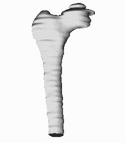
61 Fig. 5.1 Fig

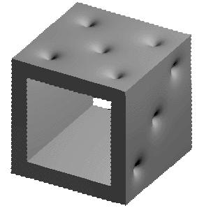
62 Fig. 5.3 Fig. 5.4 Fig

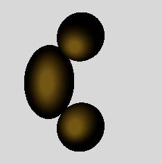
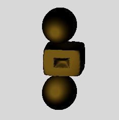
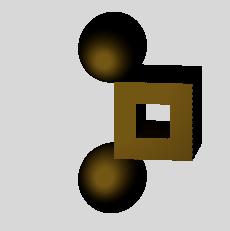
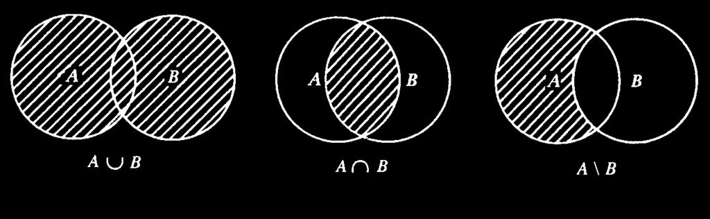
63 Fig. 5.6 Fig. 5.7 Fig

64 Fig. 6.2 Example of a CSG tree. Operations: R (rotation), \ (subtraction), (union). B-rep Face F k Vertex V i F 1 F 2 F 3... Face list Edge E j F 2 E 3 V 3 E 1 E 2 E 3 E 4... Edge list V 4 F 1 E 4 E 2 V 1 V 2 V 3 V 4... Vertex list V 2 V 1 E 1 (x 1,y 1,z 1) (x 2,y 2,z 2)... Vertex coordinates Fig

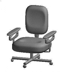
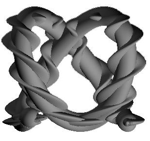
65 Fig. 6.4 Fig. 6.5 a b Fig

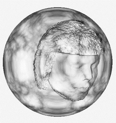
66 Fig. 6.7 Fig. 7.1 Fig