Modelling species distributions for the Great Smoky Mountains National Park using Maxent

Transcription

1 Modelling species distributions for the Great Smoky Mountains National Park using Maxent R. Todd Jobe and Benjamin Zank Draft: August 27, Introduction The goal of this document is to provide help for managers and researchers at Great Smoky Mountains National Park (GRSM) in modelling species distributions using maximum entropy (maxent) methods. It provides a reference for the maxent software (Phillips and Dudik 2008): the standard for modelling species distributions. Below is a brief background on maxent and the motivation for its use in GRSM. In the sections following we provide help for: getting the software, preparing data for use in the model, running the model, and creating a binary range map from the model. This document is designed to supplement, not replace the help files contained in the maxent software. It is strongly recommended that users also read (Phillips et al. 2006), (Phillips and Dudik 2008), and the tutorial.doc, which is packaged with the maxent software. Also, this document is structured for users working on a Windows system that has an installation of ArcGIS (ESRI 2006), though maxent can be run equally well on other operating systems (2) and with other GIS software. 1.1 Motivation and Background Modeling of species distributions in parks holds many values for the scientific community, but for stewardship of park resources by the NPS, it is critical. Only having species occurrences as points is of limited usefulness to park managers, since they cannot infer what is between the points. Knowing with some probability where species are in large natural areas is essential to taking actions to protect them, including monitoring, stewardship of rare species, reacting to a species that is suddenly found to be at-risk, and modeling future scenarios that place species in jeopardy. Currently there are many threats to natural systems and native species at Great Smoky Mountains National Park. The biological complexity, interactive stressors and limited agency resources at the Smokies, make knowing where to take the most e ective actions imperative. Maxent is a method for generating predictive distributions given a set of occurrence data and known environmental variables at those locations. This predicted distribution is constrained such that it is close to the empirical average of environmental variables at the occurrence locations. Among all possible models that fulfill these constraints the model of maximum entropy is the model which fits only the minimum constraints (i.e. it avoids over-fitting by choosing the most unconstrained model possible given the constraints set by the environmental variables at presence locations). Maxent has been used extensively is physics and economics applications. It is just one among many di erent options for generating species prediction distributions using environmental variables at species presence site (GARP, GLM, GAM), but has several advantages. Taken from 1

2 Phillips et al. (2006), maxent 1) requires only presence data, not presence/absence data, 2) can use both continuous and categorical variables, 3) the optimization is e cient, 4) has a concise probabilistic definition, 5) it avoids over-fitting through l1-regularization, 6) can address sampling bias formally, 7) output is continuous (not just yes/no), and 8) is generative rather than discriminative which makes it better for small sample sizes. There is some criticism against using Maxent for species distribution modelling. Specifically, Maxent considers only presence data instead of both presence and absence data. As a result, capture probabilities are not explicitly included in the model. This is nearly anathema in the field of Wildlife Biology where predictions based on mark-recapture studies have been the norm for years. There are at least 3 practical answers to this criticism. The first is to be explicit about the prediction probabilities that maxent produces. Rather than modelling the probability of an occurrence, maxent models the probability that an occurrence at a given location is di erent from a randomly selected location. The di erence from true occurrence prediction is subtle, and in many cases probably does not matter. Second, outside of animal studies, presence data, not presence/absence data or multiple observer data, is the norm. We know of no published data on plants where multiple observers were used to assess the observation probability of a species. Longitudinal studies are common, but they are not used in the same way that mark-recapture studies are used with animals. Finally, because of the advantages outline above, maxent is the easiest model to implement for the large amount of species that must modeled in the GRSM. Developing an inhouse model with all the advantages of maxent that includes both presence/absence data would be extremely costly. It is likely that support for presence/absence data will be included in future version of maxent, at which point the predictions surfaces can easily be recalculated without the cost of developing an in-house solution. 1.2 Document Conventions This document contains source code, windows-specific mouse-click sequences and other special formats. The table below summarize these typesetting conventions: Font Click Command File Variable Behavior Windows buttons or fields Command Line or field input File or directory name Replace with user-defined name When multiple clicking tasks are performed in a sequence, they are connected with a!. 2 Getting the Software There are many di erent software packages that can optimize data using maximum entropy methods. In this document, however, we focus on the most common software package for biologists (Maxent). The software is available for download at schapire/ maxent/. The program is written in Java. This makes it cross-platform, which means that the code runs equally well on Unix, Macintosh and Windows operating systems. Most computer systems come with the Java run-time environment pre-installed or it is download Java during the course of Internet use. To see if Java is installed: 2

3 Open a terminal Start! Run! cmd type: java -version. If the above command returns an error, then Java is not properly installed. It can be downloaded from The main file to consider once the maxent files are downloaded from the website are: maxent.jar and maxent.bat. maxent.jar is the Java executable. It can be called from the command line using the java command: java -jar maxent.jar (4 ). The maxent.bat file is a windows batch file which can be double-clicked from the windows interface and starts the maxent.jar executable. Both of these files are small. When performing an analysis, it makes sense to just copy these two files into the workspace that is created to hold the data and outputs (3.2). The maxent software contains a considerable amount of help documentation available from the user interface. There is also an excellent tutorial provided at the website where maxent is downloaded. It is strongly recommended that users go through the tutorial prior to using maxent on real data. 3 Preparing the data Maxent requires precise formatting of the species occurrence data and the environmental data. Further, the spatial attributes of all data must be identical. This section is meant to guide users through the preliminary decision about species and environments that must be made, and then help users convert their data into formats appropriate for analysis in maxent. 3.1 Preliminary decisions There are some decision made up front which will alter how every other part of the analysis proceeds. Species and environmental layers must be selected which conform to certain geographic requirements, and the spatial attributes of all these layers must be defined Choose species Maxent can build models for multiple species at one time. The species to be modelled must have geolocated occurrences. It is advantageous if the precision of these geolocations are also known. Environmental maps can be adjusted to match the precision of the geolocations. If any temporally sensitive environmental data are included (e.g. temperature for a particular year, or fire history), then the species observation dates must coincide with dates for which the environmental data are valid Choose environmental variables The predictions of any model will be improved if the selected environmental layers reflect the ecology of the organism. These associations may not be known for many species beforehand, however. Including every remotely sensed variable available is another option, and maxent provides estimates of the importance for each environmental variable included in the model (5.2). Maxent also provides a tuning parameter that adjusts the degree over-fitting (4). So, the kitchen-sink approach to 3

4 variable inclusion works better in maxent than other approaches. At a bare minimum, species respond broadly to gradients of temperature and moisture. Three variables that approximate these gradients in GRSM are elevation, topographic convergence index, and hillshade (Jobe 2006) Choose a projection You must choose a projection that matches precisely among all data types. This includes having the same datum among all data types. Data layers for GRSM are typically projected as Universal Transverse Mercator (UTM) zone 17, and either have the NAD27 or WGS84 datum. WGS84 is preferred, but the choice of datum and projection does not matter as long as both the occurrence data and all the environmental are exactly the same. Projecting digital elevation models (DEMs) is not recommended if any other environmental layer is derived from them (e.g. slope, hillshade, hydrological models). The resampling required for projection introduces striations in the derived layers. It is best practice to project all other layers to match the projection of the DEM. Alternatively, derive layers from the DEM in the original projection, reproject all the grids. In ArcGIS you can use ArcToolbox to project both rasters and features. To project all layers to a common projection use the batch project option: Start ArcGIS Load all unprojected grids into the document. ArcToolbox! Data Management Tools! Projections and Transformations! (Right-click) Project Raster! Batch... Highlight each raster in the workspace and drag them to the field Input Raster. For the first raster (double-click) Output coordinate system Select a coordinate system from the box using an imported grid or browsing for a projection. Copy and paste the resulting value into each row of Output coordinate system. Repeat for Geographic Transformation if necessary. At the end you should have new set of environmental layers, all sharing the same projection. 3.2 Prepare a workspace It is simpler to create one folder for a given analysis. Here, we term this the workspace. The files maxent.bat and maxent.jar should be copied into this workspace. Also, two sub-folders should be created in the workspace: grid, which will hold the prepared ArcGrid binary environmental layers, and ascii, which will hold the prepared ESRI ASCII environmental layers. 4

5 3.3 Prepare the environmental layers The environmental layers set the geographic extent of the analysis window in the maxent software. So, it is best to prepare these layers before the species occurrence data, because some of the occurrences may lie outside this window and will have to be pared accordingly (3.4) Maxent expects environmental data to be in ESRI ASCII grid format (AAIGrid). These grids can contain either continuous, or categorical data. If the grid is categorical, each category must be coded as an integer value. Environmental layers must share the same extent, the same grain, and the same mask (i.e. NODATA cells). In short, each layer must be identical except for the values contained in the data cells. The names of each environmental layer should be less than 13 characters. Optionally, categorical layers should begin with prefix (e.g. c_). If maxent is ever run from the command line, these layers can be switched from continuous (the default) to categorical based on their prefix using the command option togglelayertype. There are many ways to ensure that the environmental layers have matching spatial attributes, but here I present a method that uses the Spatial Analyst toolbar in ArcMap. I assume that the environmental layers are already in the standard ArcInfo binary grid format and that they have the same projection (3.1.3). If some environmental layers are stored as polygon shapefiles, then they must be converted to ArcInfo binary grids from: Spatial Analyst! Convert! Features to Raster... (details for starting Spatial Analyst are given below). The cell size for the output grid may be determined beforehand, or should be taken to be the largest cell size of the environmental layers already stored as grids. 1. Begin by loading all the environmental grids as layers in ArcMap. 2. Make sure the Spatial Analyst tool bar is available. If not: Tools! Extensions! Spatial Analyst (check to activate) View! Toolbars! Spatial Analyst 3. Set the analysis environment of Spatial Analyst Spatial Analyst! Options... General Working Directory:Path to Analysis Workspace\grid Mask: <None> Extent Analysis Extent: Intersection of Inputs Cell Size Analysis Cell Size: Maximum of Inputs, or a predefined cell size that is greater than or equal to the largest cell size in your grid. 4. Create an analysis mask using the current environment in Spatial Analyst. This mask will align the NODATA cells for each of the output environmental layers. Open up Raster Calculator: Spatial Analyst! Raster Calculator... 5

6 Create a mask that is the intersection of the defined cells in each grid using the following statement: mask = [grid1 ] [grid2 ] [grid3 ]... where grid1, grid2,... are the layer names of the environmental grids (Note: The square brackets should be typed). This statement takes advantage of the fact that, when performing operations on a series of grids, even a single NODATA value in a layer will cause the output of that cell to be NODATA. This statement assumes that for a defined cell, at least one grid has a non-zero value. The resulting grid mask is stored in the grid directory of the analysis workspace and has a value of 1 where the mask is defined and NODATA elsewhere. Set the newly created mask grid to be the mask for the Spatial Analyst environment at: Spatial Analyst! Options...! General! Analysis Mask: mask 5. Duplicate your environmental layers into grids that have the correct spatial attributes. Spatial Analyst! Raster Calculator... Create new grids with the same name as the original grids in the working directory: grid1 = [grid1 ] grid2 = [grid2 ]... Raster Calculator does not actually replace the original grids. Instead, grids of the same name are created in the working directory, that have the appropriate spatial attributes. Remove the old grids from the ArcMap data frame. 6. Convert the newly created grids into ASCII grids Activate the ArcToolbox Raster to ASCII tool in Batch mode: ArcToolbox! Conversion Tools! From Raster! (Right Click) Raster to ASCII! Batch The Raster to ASCII batch window has two fields Input raster and Output ASCII raster file. Drag the grid layers from ArcMap to Input raster. Rename the default values of Output ASCII raster file to grids of the same name, but in the ascii folder: Input raster Output ASCII raster file 1 grid1 Path to workspace\ascii\grid1 2 grid2 Path to workspace\ascii\grid2... After following these steps, the ascii folder in the analysis workspace will have all of the grids necessary for analysis in maxent. ArcMap should not be closed at this point, however, because the binary grids will still need to be used. 6

7 3.4 Prepare the species occurrence data Here, I assume that all species occurrence data have been projected to match the environmental layers (3.1.3), that the data exist as a point shapefile, and that one field of the shapefile contains the species name. 1. Clip occurrences to the maximum extent. Occurrences cannot have geolocations outside of the environmental layers. To guarantee this, the occurrence data must be clipped to the environmental layer. Convert the mask grid to a polygon: Spatial Analyst! Convert! Raster to Features Input raster: Path to Workspace\grid\mask Field: VALUE Output geometry type: Polygon Generalize lines: unchecked Output features: Path to Workspace\plyMask Clip the occurrence data using the new mask ArcToolbox! Analysis Tools! Extract! Clip Input Features: Path to Occurrence Shapefile Clip Features: Path to Workspace\plyMask.shp Output Feature Class: Path to Workspace\pntOccurrences.shp 2. Add XY coordinate fields to the attribute table of the occurrence data, if they do not already exist. ArcToolbox! Data Management Tools! Add XY Input Features: Path to Workspace\pntOccurrences.shp 3. Export the species occurrences attributes table as a.dbf file. Add pntoccurrences.shp to ArcMap as a layer. Right-click pntoccurrences! Open Attribute Table Options! Export Export: All Records Output table: Path to Workspace\tblOccurrences.dbf 4. Convert the.dbf file to a.csv. Open tbloccurrences.dbf in Microsoft Excel. Delete all fields except for the Species Name, X, and Y. Ensure the fields are ordered: Species Name,X,Y. Delete the header row. Save the file as a.csv: pntoccurrences.csv The end result of creating the species occurrence data should be a comma-separated values (csv) file, pntoccurrences.csv, with three fields (no header row): species, x, & y. This is the file that will be input to maxent. 7

8 3.5 Last Steps An output folder must be created in the workspace to hold the results from the Maxent model (an easy folder name is output. Optionally, you may also generate an samples with data (SWD) file for the species and the environment. Details of this format are given in the maxent tutorial, but basically it saves model run time if the environmental data at the sample points is added to the species occurrence file. Maxent optimizes the relationship between occurrences and environment using a random sample of 10,000 random points. You can skip this step in the Maxent model run by doing it yourself in ArcGIS. The procedure for generating SWD files for the observations and the environmental data is this: 1. Download and install Hawth s tools ( php). 2. Run the tool Intersect Point Data Point file to intersect:your species vector layer Raster: Select all environmental layers 3. Export the species vector layer as a *.dbf and then as a *.csv file as described in Generate a point shapefile containing 10,000 random points within the mask layer from Arc- Toolbox. Data Management Tools! Feature Class! Create Random Points Output Location : path to workspace Output Point Feature Class : environ Constraining Feature Class : mask Number of Points : Long, Add XY coordinates as in Extract the environmental data to the environ layer using the Intersect Point Data tool as above. 7. Export the environ shapefile as a *.dbf and then as a *.csv file as described in 3.4 The end result of these steps will be two files, species.csv and environ.csv. These can be loaded as the species and environmental files, respectively, in the Maxent GUI or specified at the command line (4). Maxent will still need to use the contents of the ASCII folder for generating prediction layers if that option is selected. 4 Running the Model Maxent may be run both from a graphical user interface (GUI) and called from the command line. It is suggested that preliminary analyses be done on the GUI, while larger analyses be done on the command line. Given that the species and environmental data have been generated following the instruction in 3, setting a model run on the GUI is relatively straightforward. 8

9 Figure 1: maxent GUI with settings for Hooded Warbler (Wilsonia citrina). All possible outputs are selected 4.1 Model Parameters The simplest configuration of Maxent requires only setting the path to the species *.csv file, the environmental layers folder (ASCII), and an output folder (which must already exist). All configurations of maxent are discussed below. Sample This field should contain the path to the species occurrence csv file prepared according to 3.4 (Fig. 1). This file can contain multiple species in a single file and have the environmental data included in SWD format (3.5). When a file is selected, the contents are read and the species appear in the box. A subset of species can be selected using the checkboxes. It should be noted that when multiple species are included in one sample file, the output is split by species. The outputs are not combined into a single file save for maxentresults.csv (5) Environmental Layers This field contains the path to the folder containing the environmental layers prepared in 3.3. Alternatively it may contain the path to an environmental SWD file (3.5). As with the samples file, the environmental layer names are read into the window below the directory field. You should change the continuous parameter to categorical for any environmental variables 9

10 that fit this description. Maxent fits categorical variables using a di erent function than continuous variables. Features On the left of the window are checkboxes for the types of functions that may be fit to each environmental variables. By default, auto is select. This option should be left as is, unless there is a specific reason to change it. See the tutorial or help files for a more detailed explanation of the possible fitted curves. Output Parameters The other settings available from the main screen of maxent control the type of output that is generated by the model. They are located on the lower right-hand side of the main window (Fig. 1). Their e ects are summarized below. Create response curves If checked, then response curve of the species for each environmental variable in the model are added. Make pictures of predictions If checked, then the output html file will contain an image of the prediction surface Do jackknife to measure variable importance Tests for the relative importance of each variable in the model and outputs the results to the html file. Output format The type of prediction output by the model. One of Logistic (where values are the probability of observing a species given the suitability of that environment), Cumulative (% of the maxent distribution at or below the current prediction) or Raw (the probability of observing a species in that particular pixel). Logistic output is the default and is the easiest to interpret as a measure of habitat suitability. Output file type The type of prediction grid to be created. You may choose from ESRI ASCII Grid (.asc), a slightly smaller maxent format (.mxe), a grid file for use by image processing software (.grd), or a band interleaved by line file (.bil)..asc is the default format, and it is best to leave it as such unless there is a specific reason for using the other formats. Output directory The folder to which output will be directed. This folder must be created ahead of time (3.5). Once the model is run, the most important files in this folder will be the ones with an html extension. Projection layers directory/file If you specify environmental data as sample points in swd format (3.5) you can have the output model projected onto larger grids located in the directory specified in this field. This allows model optimization to proceed rapidly, yet still provide predictions for a large extent. If environmental data are not in swd format, leave this field blank. 4.2 Advanced Settings The Settings button at the bottom of the maxent window provides access to some more customizable features of maxent (Fig. 2). A brief summary of these setting follows, though most users should leave the default settings. The exception is Random Test Percentage which should be set for most modeling scenarios. More detailed explanations can be found in the maxent tutorial and in (Phillips and Dudik 2008). 10

11 Random seed When checked, maxent will choose a di erent set of environmental samples to optimize the model in each run. When unchecked, the same sample will be used for each model. Logscale raw/cumulative pictures When checked, output is displayed on a log scale. This is often better for modelling rare species where much of the habitat is unsuitable. Give visual warnings When checked, maxent reports any problems encountered during the model run. Ask before overwriting When checked, maxent will ask before overwriting output from previous model runs. Show tooltips When checked, help is shown when the pointer is placed over a field or button. Remove duplicate presence records If you wish to reduce sampling bias and have duplicate presences at a given location, maxent can remove them automatically. Random test percentage A certain number of the samples can be set aside for testing the output model rather than building the model. These tests results are included in the html file and show how many of the test samples were omitted for a given cumulative prediction threshold. Regularization multiplier This parameter controls over-fitting of the model. Lower values produce more localized results and over-fitted results. Higher values produce more di use prediction layers. Maximum iterations The maximum number of hill-climbing steps to take in order to reach convergence. Maximum entropy has a finite probability of convergence, and rarely does it take more than the default 500 steps to converge. Convergence threshold This is the predicted omission rate (i.e. the probability of the model predicting no occurrence where there actually is one). It is set by default to 0.001%. Again, lower convergence thresholds can result in over-fitting, while high ones produce more di use output. Max number of background points The number of random environmental points to train the model on. The larger the number, the longer optimization will take. Bias file If observation points are not collected randomly, then a bias file can be added. This is simple a set of points to use for the background point, that have the same sampling bias inherent in the data. Maxent has been shown to be relatively robust to small deviances from random sampling, however (Phillips and Dudik 2008) addresses this issue in greater detail. Test sample file A set of test observations can be used instead of randomly drawing a percentage from the original dataset. These test samples should be in the same format as the samples dataset (3.4) All of the parameters discussed above may be set from the command line. So, a very customized instance of maxent can be run from a batch file. See the maxent help file for details on the command line flags. 11

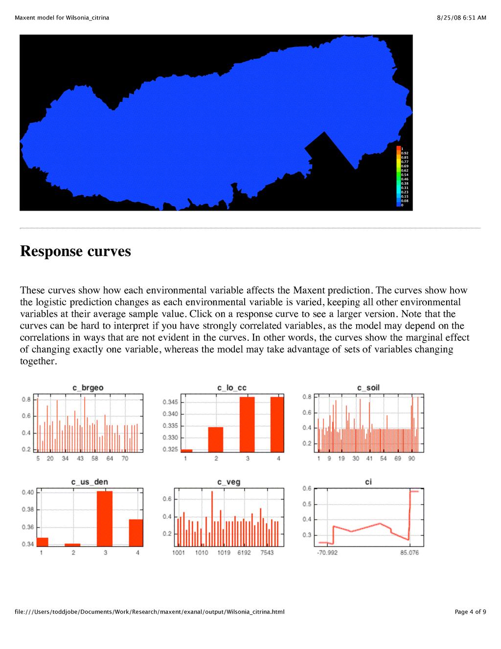
12 Figure 2: Advanced settings for maxent, set to the default Even though maxent provides many tweaking parameters, most users will benefit from leaving the default settings. The one advanced setting that can be very useful is to select a random test percentage of the data for evaluating the model. 5 Interpreting the Results Output from a maxent model run is stored in the output folder (4.1). If all output parameters are selected, then 7 files will be produced, each file name beginning with the species name. If more than one species is given in the samples file, then 7 files will be produced for each species. There is also a plot folder, which contains the raw data, and a web graphic (png) for each plot in the output. Finally, a log file (maxent.log) and a results file (maxentresults.csv) are produced. The log file contains technical output from the program which may be useful for debugging model runs that return an error, but are of little use for ecological analysis. The results file contains the raw data used to generate the html but all species are included. The most important output from maxent is contained in the html file for each species. For all discussion to follow, I have used Hooded Warbler (Wilsonia citrina) occurrences in the Park as an example dataset. The model results are generated by selecting all possible output from the model, a 10% test sample, and all other parameters set to the default. Each of these outputs is described in greater depth by the tutorial downloaded with maxent. Here, we focus on the practical interpretation of the results. We have also provided a once sentence interpretation of each graphical output from maxent (Table 1) 12

13 Output Pre- Omission vs. dicted Area vs. Pre- Sensitivity Fractional dicted Area Binary Test Table Maxent Model Projection Map Clamping Map Marginal Response Curves Individual Response Curves Variable Contributions Jackknife of Gain Interpretation Omissions Deviations from the predicted omission suggest sample bias. Background pred. Steeper curve = widespread species. Shallow = narrow. X-axis Cuto of the maxent results: varies from conservative to optimistic. Y-axis Prop. of either omissions (black, green, blue) or non-habitat (red). Model prediction good if AUC higher than random. Match between test and training curves suggests that model is equally predictive of test samples. X-axis Proportion of habitat. Y-axis Proportion of captured occurrences. Minimum training Presence Best environmental tolerance cuto. Balance... Best occurrence prediction cuto. Field. Cumulative threshold Maxent distribution cuto Logistic threshold Probability of occurrence cuto Description Cuto Scenario Fractional Predicted Area Proportion of Habitat Training Omission Rate Omitted Occurrences Test Omission rate Omitted Test Occurrences P-value Cuto model predicts better than random? Main map results of model showing areas where species is likely, and unlikely to occur. Pixel Values. Blue Low probability of occurrence Red High probability of occurrence White Training data Purple Test data Colors to the red end suggest environmental range of occurrences is small compared to the region. Limit using dontextrapolate. Pixel Values. Blue Environmental variables within model extremities Red Environmental variables outside model extremities The e ect of each variable in the mode with correlations between variable embedded. Value Correlation between occurrence and full-model environmental variables The e ect of each variable independent of the others. Value Correlation between occurrence and the single-variable environmental model. High values=important,low values=extraneous Variables which do little to decrease gain when absent (green), and have low individual gain (blue) are less important. Gain is a measure of nearness to the full model. Table 1: Summary of maxent output interpretations 13

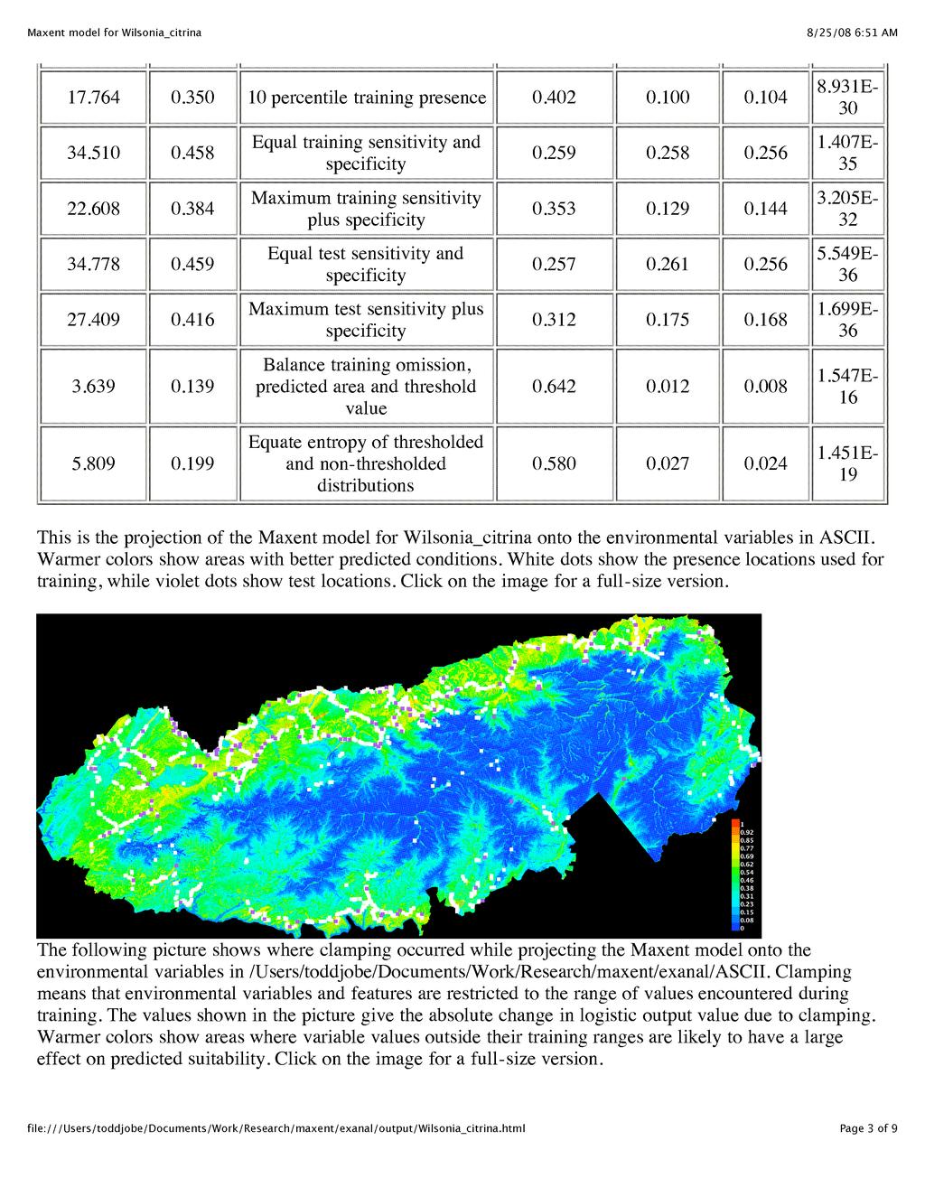
14 Some key points to remember are that the default output is on a logistic scale which means that the values reported by the model represent the probability of observing a species in a particular location. A threshold is simple the cuto value (either logistic or cumulative) that distinguished habitat and non-habitat. So, for instance a logistic threshold of 0.4 would mean that any location whose probability of occurrence is greater than 0.4 would be considered habitat, while locations with a probability less than 0.4 would be considered non-habitat. 5.1 Analysis of omission/commission This section is made of two graphs and table and two maps. Together, this output shows how well the model fits the data, and suggests thresholds for defining habitat and non-habitat Graphs The omission rate vs. predicted area graph shows omission of training and test samples as a function of the logistic threshold. Ideally, setting a cuto of 5% should eliminate 5% of the occurrences from both the test and training samples. Deviations from this suggest sampling bias in the training and/or test datasets. The ROC graph has as its x-axis the fractional predicted area (the total habitat area) and as its y-axis the sensitivity or the proportion of occurrences the habitat captures. A random habitat selection should capture species occurrence at a rate equal to the proportional area of the habitat. A model that predicts better than random will have training and test curves that lie above the random curve. Stated another way, a good mode will have a large area under the curve (AUC) for the training and test data. These curves are sensitive to species abundance, so they should not be compared among species Table While the two graphs provide qualitative analysis for the model, the table in this section provides the most useful information. It lists the results from a binomial test for a suite of di erent cuto s. The test hypothesis is that the model with a specific cuto captures the test points no better than a random model or similar area. For the Hooded Warbler example, every cuto is significant (P-Value 0.05). So, in this case every cuto scenario provides a better than random prediction of species occurrences. The choice of cuto really depends upon the purpose of modelling exercise. The threshold defined in minimum training presence statistics ensures that the model captures all training data. This is e ectively a species potential distribution; everywhere the species could survive in the environment based on the samples. The Equal training/test sensitivity and specificity balances correctly predicted occurrence with the total area of occurrence. This cuto for the Hooded Warbler was approximately 26%, which mean 26% of the Park is predicted habitat and 26% of the species occurrences are captured by the model. The best models to use for developing range maps are the last two in the table. Balance training omission, predicted area and threshold value uses empirically derived constants to weight each of these model characteristics to find the best cuto. Finally, Equate entropy of thresholded and non-thresholded distributions find the cuto results in a model most similar to the unconstrained one. After selecting a cuto from the table, a new binary map of the species predicted area can be produced (6). 14

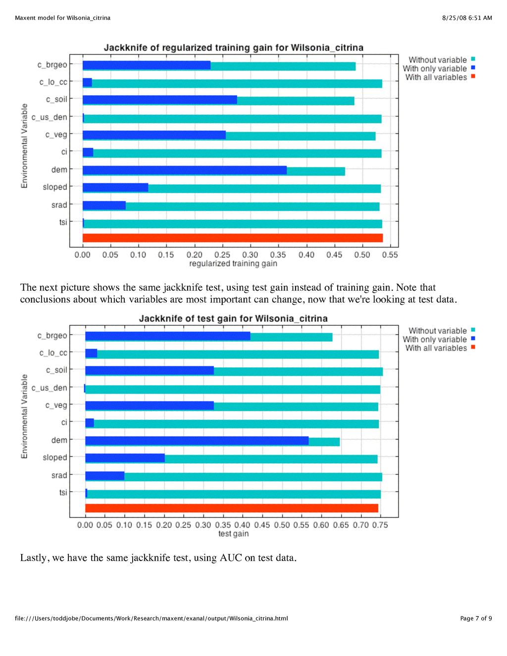
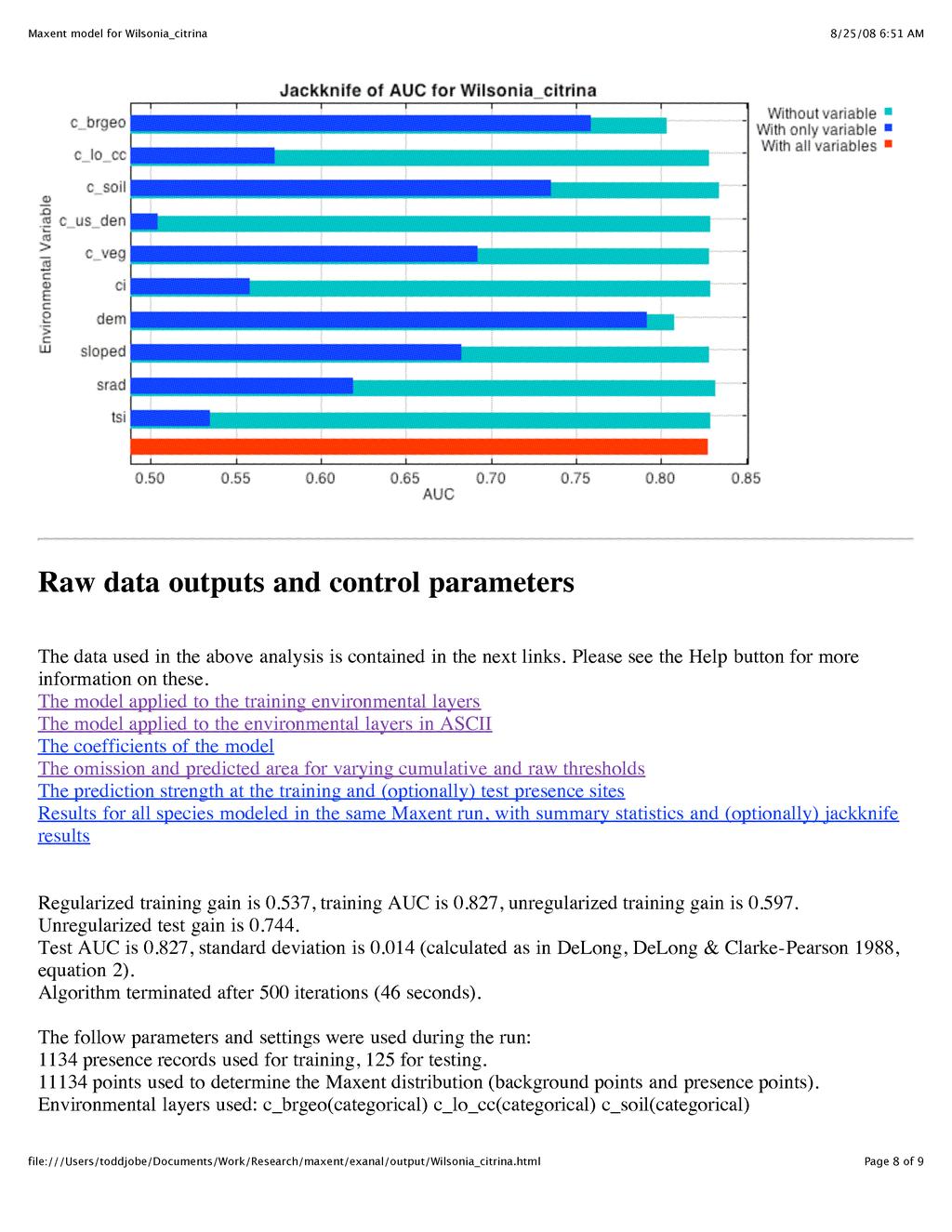
15 5.1.3 Maps Following the table of thresholds is an image output of the model projected onto the spatial analysis window. The colors represent the logistic value of the model for the environment at any location. Remember that this value represents the probability of observing a species in a given location. For rare species, much of the window may have low probability, and choosing logarithmic output from the model settings may provide a better image (4.2). The second image shows which areas of the analysis windows lie outside the range of environmental variables encountered in the training data. The image for the Hooded Warbler model is virtually all blue, suggesting that the training occurrences cover a wide range of environments in the Park. If there is a lot of red in the image, then it is unlikely the model is performing well for the entire analysis window. The model should be restricted to only the range of environments actually observed in the training data using the command line switch dontextrapolate. 5.2 Response Curves The response curves section provides information on each environmental variable and the training occurrences. The first set of graphs shows the relationship between occurrence and the environmental variable for the full model. Categorical variables are represented as bar graphs, while continuous variables are line graphs. This information can be di cult to interpret because correlations likely exist between some of the environmental variables. The second set of graphs is more useful, and show the independent relationship between occurrence and the environmental variable. If the curve for a given environmental variable does not change between the two sets of graphs, then it likely has little correlation with other variables. If however, the two graphs for a particular environmental are di erent, then correlations with other environmental variables likely exist. 5.3 Analysis of variable contributions This section begins with a table ranking environmental variables by importance in the model. For the Hooded Warbler model, elevation seems to be the most important variable. Again, however, this could be confounded by correlation among variables. The fact that the dem lines do not change between the upper and lower sets of of graphs in the response curves suggests that correlation is likely small. The graphs following the table show the changes in model performance when each variable is left out of the full model and when the variable is used by itself. Put simply, important variables will reduce the green bar, and have a large blue bar. If this trend is repeated for the graph using the test instead of the training data (i.e. the second graph in the series), we have greater confidence in the jackknife results. Finally, the e ect of selective removal and additional on the AUC is shown. It should have similar results to the graphs preceding it. Initial model runs may include many variables, and one task may be to simplify the suite of variables used in the final model. Variables that are good candidates for exclusion have the following characteristics: 1. Percent contribution based on the table is low 2. The jackknife gain for the model with only that variable (blue bar) is small 3. The jackknife gain for the full model with only that variable removed (green bar) is large 15

16 In the Hooded Warbler example tsi, c lo cc, c us den, and ci, could all be removed without much change in the final model. If the gain for the full model without the focal variable is large and the gain for the model with only that variable is also large, this suggests that the variable is strongly correlated with some other variable in the model. 5.4 Raw data outputs and control parameters This section contains links to the statistical data used to generate each figure in the html file. These data can be used in further statistical analyses on the model output. At the end of the html file the model settings used in that run are shown. 6 Creating a Range Map A desirable model output not included in the standard html output is a binary range map for the species. This map has only 2 categories, habitat and non-habitat. The delineation of habitat must be chosen by the user based on the binomial test results in the Analysis of omission and commission section (5.1). As an example, we chose a Balanced training omission, predicted area and threshold value threshold for the Hooded Warbler model. The logistic threshold was Our task is to create a binary map from the original logistic projection map where values greater than are true (1) and values less than are false (0). The procedure follows: Import the output logistic ASCII grid into ArcMap. ArcToolbox! Conversion Tools! To Raster! ASCII to Raster Input ASCII raster file: path to output folder/species name_ascii.asc Output raster: path to output folder/pred_species abbrev Output data type (optional): FLOAT Set Spatial Analyst Workspace to output folder Spatial Analyst! Options...! General Working Directory: path to output folder Compute the logical comparisons Spatial Analyst! Raster Calculator hab_species abbrev = pred_species abbrev > threshold OK After following the above recipe, the resulting grid will be in Arc binary grid format and have a value of 1 for habitat pixels, 0 for non-habitat pixels, and NODATA for pixels not inside the analysis mask (Fig. 3) 16

17 Figure 3: Range map of the hooded warbler in GRSM. Red is habitat, yellow is non-habitat. References ESRI, Arcgis 9.2. Jobe, R. T., Biodiversity and scale: Determinants of species richness in Great Smoky Mountains National Park. Ph.d., The University of North Carolina at Chapel Hill. Phillips, S., R. Anderson, and R. Schapire, Maximum entropy modeling of species geographic distributions. Ecological Modelling 190: Phillips, S. J. and M. Dudik, Modeling of species distributions with maxent: new extensions and a comprehensive evaluation. Ecography 31:

18 Appendix: Wilsonia citrina.html 18

19 19

20 20

21 21

22 22

23 23

24 24

25 25

26 26

27 27