Expander 7.2 Online Documentation

Transcription

1 Expander 7.2 Online Documentation Introduction... 2 Starting EXPANDER... 2 Input Data... 3 Tabular Data File... 4 CEL Files... 6 Working on similarity data no associated expression data... 9 Working on Gene Groups with no associated expression data ChIP-Seq Data Preprocessing GE Data Gene Expression Data Plots Differential Expression Analysis Defining a group according to a rule Defining a group according to similarity to a selected probe Clustering GE Data Hierarchical Clustering and Visualization Clustering solution cleaning Biclustering GE Data Network Based Grouping of GE Data Integrative analysis of ChIP-Seq and Gene Expression Data Group Enrichments Analysis Tools Functional Analysis Promoter Analysis Location Enrichment Analysis mirna Targets Enrichment Analysis ChIP-Seq Enrichment Analysis Pathway Enrichment Analysis General Enrichment Analysis Network Based Enrichment Analysis Gene Set Enrichment Analysis (GSEA) Matrix Visualizations PCA Transformation Analysis Wizard Additional Options File Formats Sample Input Files Supplied Files Settings R External Application Manually installation of R packages FAQ Copyrights Information References

2 Introduction EXPANDER (EXpression Analyzer and DisplayER) is a java-based tool for analysis of gene expression data. It is capable of (1) preprocessing (2) visualizing (3) clustering (4) biclustering and (5) performing downstream analysis of clusters and biclusters such as functional enrichment and promoter analysis (i.e. analysis of gene groups for enrichment of transcription factor binding sites in their promoters). EXPANDER incorporates several conventional gene expression analysis algorithms and custom ones that have been developed in the computational genomics group in Tel-Aviv University, and provides them with an easy-to-operate user interface. EXPANDER versions are available for Windows OS and for Linux/Unix OS and require the pre-installation of the Java Runtime Environment (JRE) 5.0 or later (Expander 6.05 is the first version that fully supports java 1.7). The Java Runtime Environment can be installed via: The CEL file preprocessing and the newly added SAM filter utilities require the pre-installation of one of the recent versions of R, a free software environment for statistical computing and graphics. For installation instructions, please refer to R External Application section. For improved network visualization please install Cytoscape or higher. Cytoscape can be installed via Starting EXPANDER Double click on the Expander.bat file, which is located under the Expander directory (alternatively, in Linux, open a Terminal window, cd into the Expander directory, and run the command:./expander.bat ). When running on Linux/Unix OS, make sure that you have rwx permissions for the Expander directory and for the directory in which your data is located. Also make sure that you have rx permissions for all *.exe files that are under your Expander directory. Upon running the program, the main menu bar appears:

3 Input Data Expander operates on the following types of data: a) Gene expression data For most of EXPANDER's steps for analysis of gene expression data, the technique used for obtaining the expression estimates doesn't make a difference. Whatever technique (e.g., expression arrays, RNA-Seq) was used, the input expression data should be summarized in a matrix (tab-delimited txt file; see File Formats section) in which rows correspond to probes/genes and columns to samples. Values can be either relative intensities data, expected as log 2 (R/G) values data (e.g. cdna microarrays), RNA-Seq counts OR absolute intensities data, expected as positive expression levels (E.g. High-density oligonucleotide data). Oligonucleotide data can be loaded with/without detection calls. Affymetrix data can also be loaded from CEL files (If R is installed).

4 When analyzing RNA-Seq data, one way to obtain gene expression matrix is to use TopHat ( ) to align the sequenced reads to the relevant genome, and then use Cufflinks ( ) or HTSeq ( ) to obtain gene (or transcript) expression estimates from TopHat output. If one wishes to perform functional analysis or promoter analysis, an ID conversion file should be loaded along with the data file. The conversion file maps each probe ID (first column) in the data file into a corresponding conventional gene ID that is used in the GO annotation and TF fingerprint files that are supplied with EXPANDER. The conversion file can be loaded in the middle of the session too, by Data >> Load Conversion File. b) Similarity data a pre-calculated similarity matrix c) Gene group data contains predefined groups of genes. In this data type, the conventional gene IDs that are used by EXPANDER in the GO annotation and TF fingerprint files are expected. For details regarding the Gene ID convention that is used for each organism, refer to the Supplied Files section. For details regarding the data files formats see the File Formats section. d) Gene Ranking Analysis (GSEA) contains predefined ranked genes. In this data type, the conventional gene Ids that are used by EXPANDER in the Gene Set Enrichment Analysis are expected. For details regarding the data files formats see the File Formats section. e) ChIP-Seq data contains discovered peaks of Transcription Factor(TF) ChIP-Seq experiment in BED or GFF3 formats (see File Formats section). Loading gene expression data: Tabular Data File To load tabular expression data, select: File >> New Session. From the submenu select Expression Data >> Tabular Data File. When selecting Tabular Data File, the following dialog box will appear:

5 Data type and scale are to be determined according to the input file. If the file contains missing values, these values will be estimated upon loading the data either by setting them to and arbitrary value (if the Set missing value to option is selected) or by utilizing the KNN (K- Nearest Neighbors) method (if the Estimate missing values with KNN option is selected). If the file contains Affymetrix detection calls data, the relevant check box must be checked. You may change / erase the default floor value, to which all entries that are below that value will be set (this option is available only for absolute intensities data). Advanced Input Dialog: Upon pressing the Advanced button after filling the Raw Data File field, an Advanced Input Dialog appears. This dialog box can be used in order to facilitate the data load of files that are not in the required format. The first few rows and columns of the data are displayed in a table, demonstrating the way the data is read by the program according to the current input values.

6 CEL Files To load expression data from CEL files, select: File >> New Session. From the submenu select Expression Data >> CEL Files. The load of CEL requires installation of R software (see R External Application section) along with specific packages, as detailed below. An open internet connection is also required for this operation. Expander supports CEL files of three chip types: 1. 3' Gene Expression - requires Bioconductor affy package

7 2. Whole-Transcript Gene Expression (Gene 1.0 chips) requires the prior installation of a cdf package for the used chip (see links below). 3. Alternative Splicing (Exon 1.0 chips) requires the prior installation of a cdf package for the used chip (see links below). * Please note that we estimate the overall expression for the transcript, not exon-by-exon. Therefore, this becomes 'gene data' rather than 'alternative splicing data'. When selecting CEL Files, the following dialog box will appear: Please choose the relevant organism and chip type. Then browse to the folder where the CEL files are located (Files location), and choose where to save the expression file resulting from the CEL files preprocessing. Preprocessing and normalization method: The default method in Expander is RMA. However, for 3' gene expression arrays, you may select GC-RMA instead (taking into account GCcontent bias). Before using GC-RMA, please make sure you have the gcrma R package installed (see R External Application section). CDF environment choice: You may use the default Bioconductor CDF environment for the chips or browse to an alternative CDF package which you have already installed in R. For

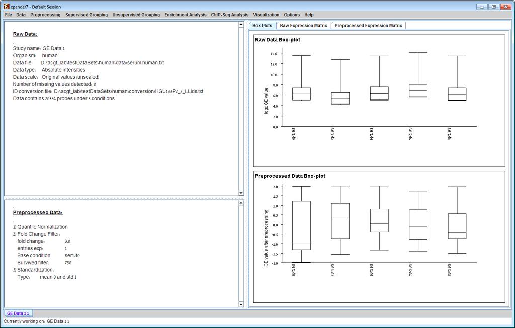
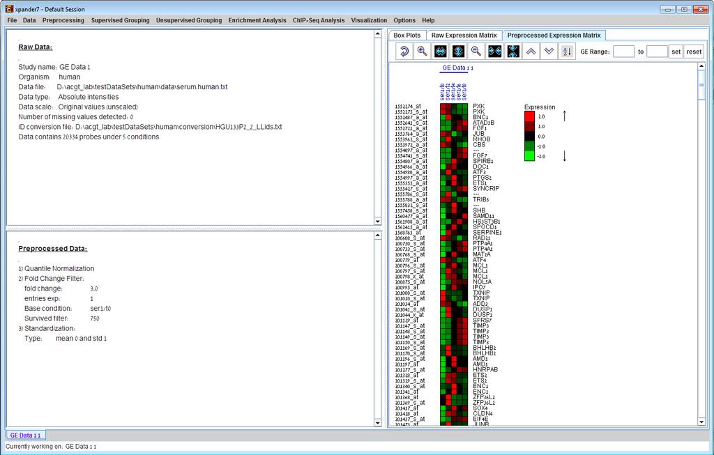
8 whole transcript and alternative splicing chips (for which there is no default Bioconductor CDF environment), you will need to supply an alternative CDF package (see links below). Note: GC-RMA requires the probe sequence information of the chip. If you decide not to use the default Bioconductor CDF environment, and have GC-RMA as the preprocessing method, you must have the suitable probe package installed in addition to the CDF alternative package. Link for downloading CDF environment packages (for 2 nd option): If Expander cannot find your R software, a window will appear, asking you to specify its location. Please browse to the location of your R software. In Windows, R.exe file is likely to be located in the 'bin' folder of R software. In Linux, you may type 'which R' in the command line to find R path. If you have a few versions of R installed, please make sure to point Expander to a version in which the Bioconductor affy package has been installed. Once the CEL files preprocessing is done, a corresponding tabular data file is generated and a 'Load Study' dialog will appear, as in loading Tabular Data. After loading a gene expression data set, a Session Data display tab is added to the main window (see example below). It contains information regarding the raw data file, a box plot chart, and an expression matrix visualization of the raw data. If detection calls exist in the data file, their statistics for each probe appear in 3 columns in the heat maps (expression matrices), in a scale between 0 and 1, corresponding to the relative part of each of the detection calls (P, M and A). The detection calls statistics for each condition are displayed in a separate tab in two tables (one for the raw data and another for the preprocessed data) and are presented in percent.

9 Working on similarity data no associated expression data To start working on similarity data (no expression data associated) select File>>New Session>> Similarity Data... The following dialog box will appear: For details regarding the data files formats see the File Formats section. After loading gene groups, a Similarity Data display tab is added to the main window

10 Currently similarity data can only be clustered using the Hierarchical clustering procedure by selecting Unsupervised Grouping>>Hierarchical Clustering>>Cluster... The resulting tree can be used to generate groups (for further details see Hierarchical Clustering). Working on Gene Groups with no associated expression data To start working on gene groups (no expression data associated) select File>>New Session. From the submenu select Gene Groups. The following dialog box will appear:

11 For details regarding the data files formats see the File Formats section. After loading gene groups, a Session Data display tab is added to the main window (see example below). It contains information regarding the data file, and a table describing the different groups (serial number, name and size). Group names can be modified, by editing the corresponding cell in the table. Upon clicking on a row in the table, the corresponding group pane appears on the right. It contains a list of the genes in the group and a view of their chromosomal positions. If a network file has been loaded (via Data>>Load Network), the subgraph, induced by the group is displayed as well.

12 ChIP-Seq Data To load ChIP-Seq data, select: File >> New Session. From the submenu select "ChIP-Seq Data". The following dialog box will appear:

13 Select the organism and its reference genome that correspond to the ChIP-Seq experiment. For details regarding the data BED/GFF3 files formats see the File Formats section. Gene hit range: This option allows choosing the gene range to be searched for peak hit. The range is selected in the following way: Start position upstream to the Transcript Start Site (TSS) and end position downstream to the TSS or to the Transcript Termination Site (TTS). Note that the start position is a non-positive value. There is an option to select more than 1 closest gene to peak by changing "Selecting top k closest genes" field and to set a distance bound for k>1 closest gene to peak. After loading a ChIP-Seq data, a ChIP-Seq Study Data display tab is added to the main window (see example below). It contains information regarding the raw data file, a pie chart, a chromosome visualization of the mapped genes positions, a region hits enrichment bar chart, and a peaks annotations table. The pie chart contains the peaks distribution of the first closest gene hits. Each peak was mapped to the closest gene with regard to the TSS and mapped to one of the following regions: Upstream of the TSS, 5UTR, Exon, Intron, 3UTR, Downstream of the TTS or Intergenic (i.e., regions between genes). Chromosome visualization displays mapped genes to peaks with option to show or not to show the gene's strands. Region hits enrichments displays the enrichment test using binomial p-value was performed in order to evaluate the randomness of peaks falling in a specific region (excluding "Intergenic" region), for example, it can be seen that under 5UTR bar, peaks fall by random in this region with p-value 3.87E-133. This option is currently available only for human and mouse datasets.

14 The peaks annotation table (see below) displays details for each peak Peak ID (row number in ChIP-Seq file), Chromosome Position of the peak with a link to UCSC genome browser, Gene ID of the mapped gene to peak (blank if the peak was not mapped to a gene), Gene

15 symbol, UCSC Transcript ID, Strand, Distance from TSS (negative/positive for upstream/downstream), Sequence type for the peak's mapped region and Intensity" or "Qvalue" depending on the uploaded file format (BED or GFF3). Pie chart, chromosome visualization and Region hits enrichment bar chart can be increased or decreased using the mouse scroll wheel. Fetch ChIP-Seq peaks sequences To fetch FASTA sequences for the peaks select ChIP-Seq Analysis >> Motif analysis >> Fetch ChIP-Seq Sequences. The following dialog box will appear: Select the directory path where the created files will be inserted (Default folder is

16 <path to>/expander/organisms/<selected organism>/chipseqsequences/). Sequence parameters: Please see image demonstration below. Sequence Width - by selected width (Default is 300 bps) or by peak width. Upstream/Downstream base pairs jump (Default is 500 bps) For each peak, two background sequences of length 300 bps are created 500 bps upstream and downstream from the middle position of the peak. Use masked sequences Fetch sequences from repetitive masked FASTA genome. Select number of peaks: Top number of peaks top peaks are selected by their score (Intensity or q- value). If the no score was added then the peaks are selected according to their row line position in the file. Peak minimum score available only in BED format. Peaks are selected if their score is above the selected minimum score. Maximum q-value available only in GFF3 format. Peaks are selected if their q-value is below the selected maximum q-value. Option to perform AMADEUS De-Novo motif finding: If selected then after creating the sequences the following AMADEUS dialog box will appear: The created 3 files will be filled in the relevant 'Input Files' fields. Under 'Parameters' a search region upstream/downstream with respect to the middle peak and a motif length should be defined. After clicking 'OK', An Amadeus visualization will be created. For further explanation on the visualization please refer to AMADEUS section. After clicking OK, 3 files will be created in the selected folder:

17 sequences.fa contains the FASTA sequences of the selected peaks and their two background sequences. target.txt contains identifiers of the selected peaks. background.txt contains identifiers of the selected peaks and their background identifiers. Notes Fetching non-masked sequences process should take on average ~1-2 seconds for about ~5000 sequences of length 300 bps. Fetching masked sequences might take longer time on average ~10 seconds for ~5000 sequences of length 300 bps. Preprocessing GE Data The following preprocessing operations can be performed using EXPANDER: 1) Flooring (Preprocessing >> Floor Data): setting all expression values that are below a certain threshold (set by the user) into that threshold. This can be done either by setting the floor value itself, or by setting the percentile that should be used as floor value. 2) Merging conditions (Preprocessing >> Merge conditions): merging a selected set of condition profiles (columns) in the dataset into one profile, in which each entry holds the average value of the merged entries. 3) Merging probes according to gene ID (Preprocessing >> Merge Probes by Gene ID): automatically shrinks the matrix so that all rows of probes from the same gene are merged into one average row, identified by the corresponding gene ID. 4) Normalization: required in order to remove systematic variation, i.e. variation arising from reasons other than biological differences between RNA samples. Expander performs normalization only for absolute intensities data, since it is assumed that the relative intensities data (e.g. cdna microarrays) is already normalized, as it is input after performing log ratio (log2r/g). Normalization can be performed using the following schemes:

18 a) Quantile normalization (Preprocessing >> Normalization >> Quantile), in which the whole data is used. b) Non-linear baseline normalization (Preprocessing >> Normalization >> Non Linear Baseline), which uses a baseline array (can be selected by the user). In this scheme a normalization function is calculated using pseudo Loess regression of the M vs. A scatter plot. The subset of genes that are used to evaluate the normalization function can be set to all genes (recommended when most genes in the dataset are expected to be constantly expressed) or a rank invariant set of genes (recommended when there can be a large number of differentially expressed genes). For more details regarding the normalization schemes see the References section. 5) Condition filtration: the conditions used in the analysis can be manually filtered by selecting: Preprocessing >> Filter Conditions. This will bring up a dialog box in which the user can select the required conditions from a list. 6) Gene (probe) filtration: can be performed in order to filter out some of the constantly expressed genes, and perform downstream analysis on a smaller informative subset of the genes. Probe filtration can be performed using the following schemes: a) t-test (Preprocessing >> Filter Probes >> t-test): When using this method, only probes that demonstrate differential expression between two condition subsets are selected. b) SAM - Significance Analysis of Microarray (Preprocessing >> Filter Probes >> SAM): selects probes that demonstrate differential expression between conditions subsets. You may choose 2 or more subsets (multi-class tests are supported). This method uses permutations to get an empirical estimate for the FDR of the reported differential genes (for details see the References section). Before using SAM, please make sure you have R software along with the samr package installed (see R External Application section). c) Fold Change (Preprocessing >> Filter Probes >> Fold Change): when using this method only genes that are over/under expressed by at least n fold in at least k arrays are selected (n and k are determined by the user). The fold change can be calculated in relation to (a) a selected baseline array (b) the minimal expression value of the gene OR (c) the reference value when working on relative intensities (depending on the user s selection). d) Variation (Preprocessing >> Filter Probes >> Variation): In this method, the k most variant genes are selected (k is determined by the user). Variance is used to measure variation for relative intensities data, and Coefficient of Variation is used to measure variation for absolute intensities data.

19 e) Detection calls (Preprocessing >> Filter Probes >> Detection calls): in this method probes/genes are filtered according to the number of expression signals for which the detection call is P (Present). It can only be operated if the data file contains detection info. f) Load Probe Subset (Preprocessing >> Filter Probes >> Load Probe Subset): the filtered set is loaded from an external txt file (for details regarding the format please see the File Formats section). 7) Divide by Base (Preprocessing >> Divide by Base) Divides each entry in a profile (a column) by the corresponding entry in the profile of a selected base condition. This can be done for all conditions or for subsets of the conditions. 8) Log data (Preprocessing >> >> Log Data) Performs log2 operation on each entry 9) Standardization: When expression values between different genes are very different, but general expression patterns are similar (high Pearson Correlation values), we would expect to see this similarity when looking on a pattern display. Since the absolute values of expression are different, a manipulation is required, in order to view the patterns on the same scale. This manipulation is called standardization. Standardization can be performed using the following schemes: a) Mean 0 and Variance 1 (Preprocessing >> Standardization >> Mean 0 and Variance 1) normalizes each expression pattern to have a mean of 0 and a variance of 1. This method is appropriate in most cases when working on genes. b) Fixed norm (Preprocessing >> Standardization >> Fixed Norm) - normalizes each expression pattern to have a fixed norm i.e. expression levels are divided by the norm of that expression vector (the root of sum of squares of that vector). This method is appropriate when different mean values or variances are expected for different patterns (e.g. when working on conditions and expecting larger variance in later phases of a response. After performing a preprocessing operation, the information regarding the operation is added to the Preprocessed Data section in the Session Data tab. In addition, the Preprocessed Data box plot and Preprocessed Expression Matrix are automatically updated according to the new values in the data.

20

21 Upon selecting Preprocessing >> Undo the data is changed to be as it was before the most recent preprocessing operation was performed, and the corresponding information is removed from the Preprocessed Data section. The Preprocessed Data box plot and Preprocessed Expression Matrix are automatically updated accordingly. All the above operations can be performed before running further analysis on the data and generating displays. When attempting to perform further preprocessing operations after analysis results and visualizations have been generated, the following dialog box appears: Upon choosing to open an additional data sheet, a new data set view tab called Data Sheet 2 is added to the main frame. The title of this tab is highlighted (colored in purple), indicating that it is now the active data sheet (i.e. all further operations refer to this data sheet). The active data sheet is automatically changed according to the selected (front) visualization tab. Preprocessed gene expression data can be saved to a file at any time be selecting Preprocessing >> Save Preprocessed Data. The data is written in the same format defined for input GE data. Gene Expression Data Plots Expander provides two types of scatter plots visualizations that can be operated via Visualization >> Scatter Plots... Simple plot - Displays a scatter plot of two arrays (selected by the user), in which the ith point (xi,yi) represents the expression value (log expression for un-logged data) of the i th gene in one array vs. the other. For normalized data, points should be located around the y=x line (marked on the scatter plot).

22 M vs. A plot (available only for absolute intensities data) - Displays a scatter plot in which each point (Ai,Mi) represents the log intensity difference of the i th probe in the two arrays (selected by the user) vs. the average log value of these intensities.

23 Differential Expression Analysis The goal in this analysis is to detect groups of genes that demonstrate differential expression between two/more condition groups. a) t-test (Supervised Grouping >> Differential Expression >> t-test): When using this method, genes can be assigned into one of two groups (up-regulated and down-regulated), depending on the definitions of t-test parameters. b) Wilcoxon\Mann-Whitney two sample rank sum test - (Supervised Grouping >> Differential Expression >> Ranksum test): When using this method, genes can be assigned into one of two groups (up-regulated and down-regulated), depending on the definitions of Ranksum test parameters. This method is nearly as efficient as the t-test on normal distributions of expression values but has a greater efficiency than the t-test on non-normal distributions of expression values. Negative binomial (DESeq2) Negative Binomial distribution test for RNA-seq count data (Supervised Grouping >> Differential Expression >> NB (DESeq2)): this method is used to

24 demonstrate differential expression between 2 condition subsets for RNA-seq count data where for each probe i and condition j in the expression matrix the value is a non-negative integer. The probes are then assigned into two groups (up-regulated and down-regulated). DESeq2 requires annotation data table file which includes the attributes/categories and their corresponding labels for each condition in the RNA-seq data. For details regarding the annotation data file format see the File Formats section. When selecting Supervised Grouping >> Differential Expression >> NB (DESeq2), the following dialog box will appear: Annotation data file should be given. Advanced Input Dialog: Upon pressing the Advanced button after filling the Annotation data file field, an Advanced Input Dialog appears. This dialog box can be used in order to facilitate the data load of files that are not in the required format. The first few rows and columns of the data are displayed in a table, demonstrating the way the data is read by the program according to the current input values.

25 For further information regarding DESeq2 please refer to References. Before using DESeq2, please make sure you have R software along with the DESeq2" package installed (see R External Application section). c) Negative binomial (edger) Negative Binomial distribution test for RNA-seq count data (Supervised Grouping >> Differential Expression >> NB (edger)): this method is used to demonstrate differential expression between 2 condition subsets for RNA-seq count data where for each probe i and condition j in the expression matrix the value is a non-negative integer. As part of the test 3 different dispersion options are given: Tagwise for a large amount of samples (>6), where a different dispersion is calculated for each probe, Common for small amount of samples (<6), where the same dispersion is given for each probe, Poisson a special case of NB where dispersion = 0 for all probes. The probes are then assigned into

26 two groups (up-regulated and down-regulated). For further information regarding edger please refer to References. Before using edger, please make sure you have R software along with the edger and "limma" packages installed (see R External Application section). d) SAM - Significance Analysis of Microarray (Supervised Grouping >> Differential Expression >> SAM): this method detects probes that demonstrate differential expression between conditions subsets. You may choose 2 or more subsets (multi-class tests are supported). The probes are then assigned into two groups (up-regulated and down-regulated) if 2 condition groups are tested or into one group of differentially expressed otherwise. SAM uses permutations to get an empirical estimate for the FDR of the reported differential genes (for details see the References section). Before using SAM, please make sure you have R software along with the samr package installed (see R External Application section). After performing differential expression grouping analysis, a solution visualization tab is added to the main window. It contains the following views: Information regarding the algorithm, number of groups (can be either 1 or 2), number of ungrouped elements (non-differential), and numerical measures of the groups quality, including: a) Overall average homogeneity - calculated as the average value of similarity between each element and the center of the group to which it has been assigned, weighted according to the size of the group. b) Overall average separation calculated as the average similarity between mean patterns of different groups, weighted according to their sizes. c) Groups table - contains the number, name (label), size and homogeneity of each group. Mean Patterns of the groups with error bars (±1 STD). Upon selecting a group, the corresponding pane is displayed on the right. It contains a list of probes, p-values/q-values, fold-change, probe patterns, expression matrix (heat map) and the chromosomal locations of the genes. Similarity matrices for probes within the cluster as well as for conditions are also displayed in this tab, if the relevant options in the display settings are selected (see the Settings section). If a network file has been loaded (via Data>>Load Network), the sub-graph, induced by the cluster is also displayed in the group pane. In order to allow comparison between groups and patterns, the displayed expression patterns are automatically standardized to have mean = 0 and STD = 1. A differential expression solution can be saved using the File >> Export to text..., and reloaded using the Grouping Supervised Grouping >> Differential Expression >> Load Solution.

27 Defining a group according to a rule This can be done by selecting Supervised Grouping >> Rule-based Grouping. The following input dialog box will appear: Upon pressing the New button, the following dialog box will appear, to allow defining the group rule:

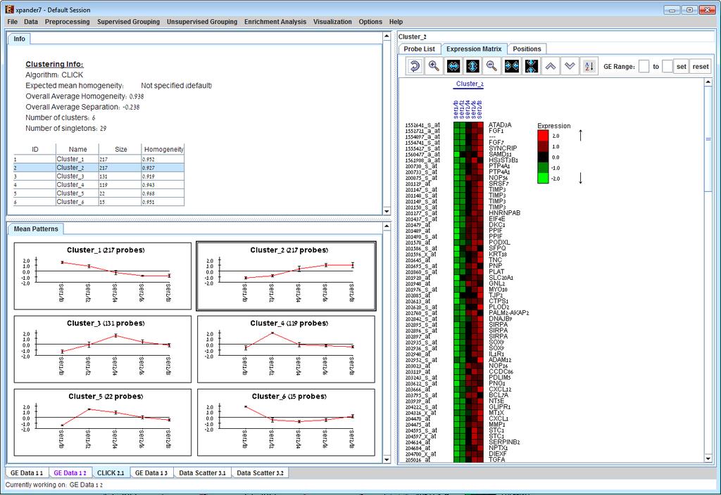
28 In the dialog box, name the new group and select the conditions of interest. For each condition define weather the expression level should be up-regulated, down-regulated or steady (between the up-regulation threshold and the down-regulation threshold). These thresholds should also be defined. A condition can also be added by pressing the All button. In this case a separate group will be defined for each of the options of that condition (i.e. a definition of a group using the All button can result in more than one group). The visualization for this operation is similar to the clustering results visualization (described below). Defining a group according to similarity to a selected probe This can be done by selecting Supervised Grouping >> Group by Pattern Similarity. An input dialog box allows setting the similarity measure (Pearson correlation, Spearman correlation or Euclidean distance) and reference probe ID as well as the expected group size. The visualization for this operation is similar to the clustering results visualization (described below). Clustering GE Data The goal of clustering is to partition the genes into distinct sets such that genes that are assigned to the same cluster should have similar expression patterns, while genes assigned to different clusters should have non-similar expression patterns. Usually there is no one solution that is the true mathematical solution for this problem, but a good clustering solution should have two merits: (1) High homogeneity (average similarity between genes from the same cluster). (2) High separation (average distance/dissimilarity between genes from different clusters). After operating one of the clustering algorithms a clustering results view appears. The view contains information about the solution and its quality including the method and parameters that were used to obtain it, number of clusters, number of singletons (probes that were not assigned to any cluster), overall homogeneity and separation, as well as the size and homogeneity of each cluster. This summary can be used to compare different solutions. In order to apply a clustering algorithm to the data, select the required algorithm from the Unsupervised Grouping >> Clustering menu (options are: KMeans, CLICK, SOM). You can also use the agglomerative hierarchical clustering algorithm by extracting a partition from an existing hierarchical tree, by selecting Unsupervised Grouping >> Hierarchical Clustering>> Generate Groups (For details about building such a tree, please go to Hierarchical Clustering).

29 Currently similarity data can only be clustered using the Hierarchical clustering procedure by selecting Unsupervised Grouping>>Hierarchical Clustering>>Cluster... The resulting tree can be used to generate groups (for further details see Hierarchical Clustering). An existing clustering solution can be loaded from a file by selecting Unsupervised Grouping >> Clustering >>Load Solution (For details regarding the clustering solution file format, refer to the File Formats section). The CLICK algorithm is not designed to find clusters under the size of 15 probes, so it might fail in clustering small datasets. Fill the required input data in the algorithm input dialog box and press the Ok button. The parameters required for each method are as follows: Algorithm KMeans SOM CLICK Hierarchical tree partition Required parameters Expected number of clusters. Grid width, grid length (width*length >= number of clusters) and number of iterations. Homogeneity value (0-1): allows the user control over the homogeneity of the resulting clustering, i.e. the average similarity between elements in the same cluster. This parameter serves as a threshold in various steps in the algorithm, including the definition of cluster kernels, singleton adoptions and kernel merging. The default value for this parameter is the estimated homogeneity of the true clustering. The higher the value assigned to this parameter the tighter the resulting clusters. Distance threshold (if extracting by distance): 0-1 the minimal tree distance that is required for two nodes to be assigned to the same group It is also possible to partition the tree according to manual node selection that is performed on the hierarchical view (see Hierarchical Clustering). Details about the algorithms can be obtained through the relevant articles in the References section.

30 After clustering is performed, a clustering solution visualization tab is added to the main window. It contains the following views: Information regarding the clustering algorithm, number of clusters, number of un-clustered elements (singletons), and numerical measures of the clustering quality, including: d) Overall average homogeneity - calculated as the average value of similarity between each element and the center of the cluster to which it has been assigned, weighted according to the size of the cluster. e) Overall average separation calculated as the average similarity between mean patterns of different clusters, weighted according to their sizes. f) Clusters table - contains the number, name (label), size and homogeneity of each cluster. The name of a cluster can be changed by editing the corresponding cell in the table. Mean Patterns of all clusters with error bars (±1 STD). Upon selecting a cluster (from the clusters table or from the mean patterns view), the corresponding cluster pane is displayed on the right. It contains a list of probes, probe patterns, expression matrix (heat map) and the chromosomal locations of the genes. Similarity matrices for probes within the cluster as well as for conditions are also displayed in this tab, if the relevant options in the display settings are selected (see the Settings section). If a network file has been loaded (via Data>>Load Network), the sub-graph, induced by the cluster is also displayed in the cluster pane.

31

32 After performing enrichment analysis (for details see the Enrichment Analysis Tools), if enrichment has been detected in the selected cluster, the corresponding histogram and analysis information are added to the single cluster view. In order to allow comparison between groups and patterns, the displayed expression patterns are automatically standardized to have mean = 0 and STD = 1. A clustering solution can be saved using the File >> Export to text option (with the corresponding clustering view as the selected tab) OR by using the File>>Save All option, which will export all solutions within a session to text and image files. A clustering solution can be reloaded using the Unsupervised Grouping >> Clustering >> Load Solution. Hierarchical Clustering and Visualization This tool uses the agglomerative algorithm to calculate a dendrogram tree for all expression patterns (probe patterns) and/or profiles (condition profiles). The type of linkage (manner in which the distance between a new node and the rest of the nodes is calculated) used in the algorithm can be set via an input dialog (for details regarding the algorithms refer to the References section). Note that it does not generate a partition of the probes to clusters. The distance measurement used in the algorithm is (1-Pearson Correlation)/2. To perform hierarchical clustering, select Unsupervised Grouping >> Hierarchical Clustering. Upon selecting this option, a dialog box appears in which the linkage type parameter, used in the algorithm can be set. After pressing OK, the algorithm will be operated both on the probe patterns and on the condition profiles. The resulting trees are displayed next to an expression matrix so that the probe tree appears vertically on the left and the condition tree appears horizontally above the matrix. The scale next to each tree indicates the range of distance values between vectors corresponding to the leaves. The tool tip indicates the distance value corresponding to the cursor location on the tree. If condition attributes file has been loaded for the analyzed dataset, a matrix representation of these attributes will be displayed below the expression matrix (heatmap). For details regarding the condition attributes file format, refer to the File Formats section.

33 Upon clicking on the vertical tree, a corresponding sub tree is highlighted (selected) and can be defined as a group by right clicking on the same location and selecting the Export group option from the right click menu. The sub tree is then added as a group of the bottom left panel of the display. Upon selecting one of the groups that have been previously defined and added to the list on the bottom left panel, the corresponding sub tree is selected. A previously selected sub tree can be removed from the list by right clicking on the corresponding group in the bottom left panel and selecting remove group. Manually selected groups can then be defined as a grouping solution by selecting Unsupervised Grouping>>Hierarchical Clustering>>Generated Groups>> From Selected subtrees. A hierarchical clustering dendrogram can be exported to a Newick format text file by selecting File>>Export to text... when the relevant solution tab is selected. Clustering solution cleaning

34 This feature allows removing elements (i.e. probes) from a clustering solution in order to obtain higher levels of homogeneity within each cluster. It can be applied on an existing clustering solution, and results in the generation of a new cleaner version of the solution. To perform cluster cleaning select Unsupervised Grouping>>Clustering>>Clean Clusters. The following dialog box will appear: In the dialog box, select the clustering solution on which the feature should be operated, specify the minimal required correlation between each probe and the cluster center and press OK. After cluster cleaning is performed, a new clustering solution visualization tab is added to the main window. The new tab will be named by the original solution with the extension cleaned by <c> where c = the correlation threshold selected by the user.

35 Biclustering GE Data Biclustering is clustering of both genes and conditions of the data into subgroups that are not necessarily disjoint. It enables the user to detect genes that are co-regulated in only a subgroup of the conditions, and does not force genes to belong exclusively to one cluster. It is useful when working on datasets which contain a large number of conditions. Expander incorporates two Biclustering algorithms: ISA (Iterative Signature Algorithm) and SAMBA algorithm (for details see the References section). Before using ISA, please make sure you have R software along with the eisa package installed (see R External Application section). In order to apply the ISA algorithm to the data select Unsupervised Grouping>>Bi- Clustering>>ISA. This operation does not require parameter input. In order to apply the SAMBA algorithm to the data select Unsupervised Grouping>>Bi- Clustering>>SAMBA. The following dialog box will appear:

36 It enables the configuration of some of the parameters for the algorithm. The following table specifies the different parameters that can be set via this dialog box: Field Use default parameters Description When checked, biclustering parameters (described below) are set automatically (this option is recommended unless the user is familiar with the parameters). The user can select one out of 6 options. The following table describes the advantages and disadvantages of each option: Robust- can Option files type Option name fast performance less memory required: Flexible handle normalization problems and non geneexpression

37 data valsp_ valsp_ valsp_ valsp_1ap valsp_2ap valsp_3ap We recommend the valsp_3ap option (set as default), since it is very flexible, and produces good results also for data that was not normalized properly or for non gene-expression data. Always cover all genes Always cover all conditions Overlap prior factor Number of responding genes to hash Maximum hash size (in MB) Maximum hash size When checked, the solution will cover each gene at least once (each gene will be included in one or more biclusters). When checked, the solution will cover each condition at least once (each condition will be included in one or more biclusters). Un checking this option will cause a reduction in the number of biclusters, and the algorithm will run faster. Can take values between 0 and 1, describes extent of overlap that is permitted between two different biclusters in the same solution. The higher this parameter is, the more strict the algorithm will be regarding adding a new bicluster (will require less overlap between the new bicluster and the existing ones). Can take values between 1 and the number of genes in the dataset. Default value is set to 100 (recommended unless data set size < 100). Has impact over the hashing stage in the algorithm. Described the maximum memory size that can be used for the hashing part of the algorithm (the whole algorithm will take up about twice this size of memory). This parameter determines the number of condition kernel options that are tested and scored in the hashing stage. It can take values from 1 to 7. The default value is 4. In datasets with many conditions raising this

38 number will significantly increase the algorithm run time (may also produce better results). Minimum hash size This parameter determines the minimal size of condition kernel in the hashing stage. It can take values from 1 to 7 and must be <= Maximum hash size. The default value is 4. Upon clicking OK in the dialog box, the SAMBA algorithm is operated on the dataset. After biclustering is performed a biclustering solution visualization tab is added to the main window. It contains the following views: a) Information regarding the biclustering algorithm, and number of resulting biclusters. g) Biclusters table contains the following information for each bicluster: serial number, name, score, number of probes genes and number of conditions. The name of a bicluster can be changed by editing the corresponding cell in the table. The score is given by the SAMBA algorithm and is size-dependent, thus, it is not recommended to use it to compare the quality of two biclusters of different sizes. The table can be filtered to display a subset of the biclusters by clicking on the Filter ( ) button in the toolbar. Filtering can be performed according to: Score, number of probes and number of conditions. Upon selecting a bicluster (from the biclusters table), the corresponding pane is displayed on the right. It contains a list of probes, probe patterns, expression matrix (heat map) and the chromosomal locations of the genes. Similarity matrices for probes within the cluster as well as for conditions are also displayed in this tab, if the relevant options in the display settings are selected (see the Settings section). If a network file has been loaded (via Data>>Load Network), the sub-graph, induced by the cluster is also displayed in the cluster pane.

39

40 After performing enrichment analysis (for details see the Enrichment Analysis Tools section), if enrichment has been detected in the selected bicluster, the corresponding histogram and analysis information are added to the single bicluster view, and a column is added to the expression matrix display for each enrichment class, stating for each probe, whether it belongs to that class. A biclustering solution can be saved using the File >> Export to text option (with the corresponding biclustering view as the selected tab) OR by using the File>>Save All option, which will export all solutions within a session to text and image files. A biclustering solution can be reloaded by selecting Unsupervised Grouping >> Bi-Clustering >> Load Solution. For a format of the solution file, please refer to the File Formats section: Network Based Grouping of GE Data The goal here is to detect groups of genes that demonstrate similar expression patterns and are also highly connected in a given interactions network.

41 In order to operate these tools, an interactions network in.sif format needs to be loaded. This can be done either by selecting Data>>Load Network or via the dialog boxes of the tools. In order to perform network based grouping Expander incorporates two algorithms: Matisse and Degas (for details see the References section). The DEGAS algorithm is relevant when the expression dataset compares two groups of heterogeneous samples (as in case-control studies). The groups detected by these tools are referred to as modules and may contain also genes that exist in the network, but are not present in the filtered GE data (referred to as Back nodes ). To use the more advanced, stand-alone versions of MATISSE and DEGAS (with higher flexibility), please refer to the Matisse home page. In order to apply the Matisse algorithm to the data select Unsupervised Grouping>>Network >>Matisse. The following dialog box will appear: It enables the configuration of some of the parameters for the algorithm: Field Beta Maximal module size Description The fraction of gene pairs that are expected to be strongly coexpressed in each module The maximum size for a detected module. Upon clicking OK in the dialog box, the Matisse algorithm is operated on the dataset. In order to apply the Degas algorithm to the data select Supervised Grouping>>Network >>Degas. The following dialog box will appear:

42 It enables the configuration of some of the parameters for the algorithm: Field Case conditions Control conditions Dysregulation direction Dysregulation significance threshold Dysregulation ratio Optimization algorithm Description The case conditions The control conditions This parameter will determine which direction of dysregulation will be sought (up/down-regulation/both). This threshold will be used to identify which genes are differentially expressed in each 'case' sample compared to the controls The minimal threshold for the ratio between the gene expression in any of the case conditions and the average expression in the control conditions. Above this threshold a case condition is designated as dysregulated. The algorithm used to identify dysregulated pathways (DPs). See the DEGAS manuscript for details. CUSP is the recommended option

43 Maximal number of modules After DEGAS identifies a significant DP, it removes it from the input data and attempts to identify additional DPs. This parameter specifies the total number of DPs that will be sought. Upon clicking OK in the dialog box, the Matisse algorithm is operated on the dataset. After running network-based clustering, the solution is displayed in a new tab, which is added to the main window. The view is similar to the clustering results display. However it contains an additional interactions view tab for each module showing the sub-network that is formed by the module. If the Cytoscape network analysis software is installed and is running, it can be used for more advanced visualizations and analysis of this sub-network by clicking on the Cytoscape tool-button ( ) placed at the top of the interactions view tab. In the display, back nodes (genes that appear in the network, but not in the GE data) are marked in pink.

44 After performing enrichment analysis (for details see the Enrichment Analysis Tools section), if enrichment has been detected in the selected module, the corresponding histogram and analysis information are added to the single module view, and a column is added to the expression matrix display for each enrichment class, stating for each probe, whether it belongs to that class. A network-based grouping solution can be saved using the File >> Export to text option (with the corresponding grouping view as the selected tab) OR by using the File>>Save All option, which will export all solutions within a session to text and image files. A network-based grouping solution can be reloaded using the Unsupervised Grouping >> Network >> Load Solution option or via Supervised Grouping >> Network >> Load Solution. For a format of the solution file, please refer to the File Formats section. Integrative analysis of ChIP-Seq and Gene Expression Data EXPANDER has a "ChIP-Seq Analysis" menu item which provides the following tools for the joint analysis after loading both ChIP-seq and gene expression data:

45 1) Examining gene expression distribution within ChIP-Seq-associated genes: this is done via ChIP-Seq Analysis >> Integration with expression data >> ChIP-Seq vs. GE analysis. Upon selecting this option, the following dialog box will appear: In the dialog box select the relevant ChIP-seq data set name, the base-condition and the test-condition, and click OK. A box plot showing the distribution of test-base GE ratios will be displayed for the set of chip-seq genes (right) and the rest of the genes in the geneexpression data set (left). 2) Extracting a grouping solution from ChIP-seq-gene-groups intersection: this is done via ChIP-Seq Analysis >> Integration with expression data >> ChIP-Seq Intersection. Upon selecting this option the following dialog box is displayed:

46 In the dialog box select the relevant grouping solution and ChIP-seq data set name, and click OK. A grouping solution visualization tab will be added to the main window. It will contain a gene-group for each non-empty intersection between a gene-group in the original solution and the chip-seq genes. Visualization is similar to clustering visualization. 3) Gene Set Enrichment Analysis: this is done via ChIP-Seq Analysis >> Integration with expression data >> GSEA. ChIP-Seq data can be selected as "Grouping solution". For further information please refer to: Gene Set Enrichment Analysis (GSEA). 4) ChIP-Seq Enrichment: this is done via ChIP-Seq Analysis >> Integration with expression data >> ChIP-Seq Enrichment. For further information please refer to: ChIP-Seq Enrichment Analysis. Group Enrichments Analysis Tools Functional Analysis Promoter Analysis PRIMA, AMADEUS Location Enrichment Analysis mirna Targets Enrichment Analysis ChIP-Seq Enrichment Analysis Pathway Enrichment Analysis General Enrichment Analysis Network Based Enrichment Analysis

47 Gene Set Enrichment Analysis (GSEA) The following analysis can be performed on gene sets, clusters, biclusters, network based modules, similarity based groups, or the filtered dataset (the analyzed set of probes as one set). Before operating any of the enrichment analysis operation (not including the General enrichment analysis ), the data files for the relevant organism should be downloaded. Download can be done by selecting Help >> Download Data for Organism. Upon starting a new session, automatic data download will be suggested if Expander did not detect data for relevant organism. Functional Analysis This tool performs basic statistical analysis on the distribution of functions of genes within each cluster. The functions of the genes are determined according to annotation files (GO), which can be downloaded from the EXPANDER download page (see the Supplied Files section). To perform this analysis, Expander utilizes the TANGO software, which performs hyper-geometric enrichment tests and corrects for multiple testing by bootstrapping and estimating the empirical p-value distribution for the evaluated sets. Before operating functional analysis the annotation files for the relevant organism should be downloaded from the download page (more details at introduction of Group_Analysis Tools). To perform the analysis, select Enrichment Analysis >> Functional Analysis >> TANGO. The following dialog box will appear:

48 The following table specifies the different parameters that can be set via this dialog box: Field Perform analysis on Include back nodes Focus on Ignore classes over the size of Description The grouping solution on which the analysis will be performed. Include genes that are part of the module' but not included in the GE data (Relevant only if the analysis is performed on modules, detected by network based algorithm) Can be used to select annotation subtypes that are of interest (Process, Function and Location). And the analysis will focus on these types only. This parameter states the level in the GO tree at which annotations are too general (class size indicates how general it is) and are thus no

49 longer interesting. Number of iterations in algorithm Background set Corrected p-value threshold The number of random sampling performed by the algorithm. Increasing this parameter, will increase runtime and will provide higher resolution on corrected p-values. I.e., corrected p-values will range between 1/<#iterations> and 1. Determines the set of genes that will be used as background in the analysis. Options are: all genes (of the relevant organism), original input data, filtered data or background set from file (see the Files Format section for details regarding the format of an external background set). A functional class will be considered significantly enriched in a cluster/bicluster if its corrected p-value is lower than this threshold. The value in this field should be at least 1/1000, since the TANGO algorithm performs 1000 bootstraps in order to estimate the corrected p- value. Upon clicking OK in the dialog box, the TANGO algorithm is operated. After functional analysis is performed a functional analysis solution visualization tab is added to the main window. It contains general information regarding the analysis, a sort-able table holding all detected enrichments (set ID, functional class, p-value, etc.) and a multi-histogram panel along with a color index (mapping each color to a corresponding functional class). The multi-histogram panel contains one histogram for each probe/gene set/group in which enrichment has been detected. Each histogram contains a column for each significant (more frequent than would be expected by random) functional class. The definition of significant depends on the user s selection of threshold p-value i.e., a functional class is considered significantly enriched in a cluster/bicluster if its corrected p-value is lower than the preset threshold p-value.

50 The height of the column is proportional to the significance of this enrichment (i.e. height = - log(raw p-value)). The frequency in set (frequency of genes of a functional class within the examined set, in %) is written on top of the column. Upon clicking on a column, a dialog box is displayed containing the class name, raw p-value, corrected p-value, and a list of the genes in the cluster/bi-cluster that belong to the class. Upon clicking on one of the gene Ids in the table, a relevant web page with information regarding this gene is displayed. The display tool tip shows the cluster number, size and homogeneity.

51 Annotation files for each organism are updated on a regular basis (for more information, refer to the Supplied Files section). The results of this analysis can be exported to a text file by selecting File>>Export to text when the corresponding view is the selected tab OR by using the File>>Save All option, which will export all solutions within a session to text and image files. Promoter Analysis PRIMA This tool identifies TFs whose binding sites are significantly over-represented in a given set of promoters (i.e. cluster or bicluster). To perform this analysis Expander utilizes the PRIMA (PRomoter Integration in Microarray Analysis) software which performs a statistical analysis on the distribution of transcription factor motifs in the promoters of genes within each cluster or bicluster. To achieve this, PRIMA uses preprocessed TF fingerprint files, which can be downloaded from the EXPANDER download-page (see the Supplied Files section), and are updated on a regular basis. For details regarding the PRIMA software see the References section.

52 Before operating promoter analysis, the TF fingerprint file for the relevant organism should be downloaded from the download page (more details at introduction of Enrichment Analysis Tools). To perform the analysis, select Enrichment Analysis >> Promoter Analysis >> PRIMA. The following dialog box will appear: The following table specifies the different parameters that can be set via this dialog box: Field Perform analysis on Include back nodes Description The grouping solution on which the analysis will be performed. Include genes that are part of the module' but not included in the GE data (Relevant only if the analysis is performed on modules, detected by

53 network based algorithm) Fingerprints file PWM file Promoter sequences file Hits range Background set Threshold p-value Multiple tests correction Save results as Automatically set according to the selection of the organism. Automatically set according to the selection of the organism. Contains the gene sequences that are used for the TF binding sites display. Automatically set according to the selection of the organism. Determines which regions of the gene are to be analyzed. The possible range depends on the investigated organism (i.e. on the information provided in the TF fingerprint files), and is specified in the Supplied Files section. Determines the set of genes that will be used as background in the analysis. Options are: all genes (of the relevant organism), original input data, filtered data or background set from file (see the Files Format section for details regarding the format of an external background set). A TF's binding site will be considered significantly enriched in a cluster if its corrected p-value is lower than this threshold. Can be set to FDR, Bonferroni or None (when set to Bonferroni/FDR the corrected p-values are the ones that are compared to the threshold p-value). When filled, the program results are saved in stated txt file. After promoter analysis is performed, a promoter analysis solution visualization tab is added to the main window. It contains general information regarding the analysis, a sort-able table holding all detected enrichments (set ID, TF binding site, p-value, etc.) and a multi-histogram panel along with a color index (mapping each color to a corresponding TF binding site). The multi-histogram panel contains one histogram for each probe/gene set/group in which

54 enrichment has been detected. Each histogram contains a column for each significant (more frequent than would be expected by random) TF binding site. The definition of significant depends on the user s selection of threshold p-value. i.e., a TF binding site is considered significantly enriched in a cluster/bicluster if its corrected p-value is lower than the preset threshold p-value. The height of a column is proportional to the significance of this enrichment (i.e. height = - log(p-value)), and the frequency ratio (frequency in set divided by frequency in background) is written on top of the column. Upon clicking on a column, a dialog box is displayed containing: TF accession number in TRANSFAC DB [TF name], p-value, % of covered promoters in cluster, relative frequency (frequency in cluster divided by frequency in background set) and a list of the genes in the cluster which contain the motif in their promoters. Upon clicking on one of the gene Ids in the table, a relevant web page with information regarding this gene is displayed. The display tool tip shows the cluster number, size and homogeneity.

55 After performing promoter analysis, TF binding sites can be viewed by selecting Enrichment Analysis >> Promoter Analysis >> View Binding Sites OR by pressing the toolbar button ( ). After selecting the gene group (cluster/bi-cluster etc.) to be viewed, a separate frame is displayed, containing a line to represent each of the genes in the group, and a colored rectangle, to represent each binding site. A color index appears on the right, mapping each color to the corresponding TF (PWM). A check box next to each of the entries in the color index allows hiding any of the PWMs, and a radio button next to each of the entries in the color index allows sorting the genes in the display according to the number of hits of the corresponding TF. The toolbar contains tools for vertical and horizontal zooming. If a sequence file had been selected via the promoter analysis input dialog, the actual sequence will be displayed when the zoom factor (scale) allows it. Promoter and TF fingerprint files for each organism are updated on a regular basis (for more information, refer to the Supplied Files section).

56 AMADEUS Another option for performing promoter analysis, is finding enriched motifs using AMADEUS. Amadeus is a tool for de novo motif discovery. It seeks for motifs that are enriched in the promoters of a target set of genes compared to the background set. Such analysis can be applied to other sets of sequences (e.g., ChIP-Seq peaks, enhancers, etc.). In order to perform motif enrichments analysis, select Enrichment Analysis >> Promoter Analysis >> AMADEUS. The following dialog box will appear:

57 The different parameters that can be set via this dialog box are: Field Perform analysis on Motifs file Promoter sequences file Motif Length Hits range Description The grouping solution on which the analysis will be performed. A matrix table of known motifs in TRANSFAC format. The default is transfac.dat, a public release of TRANSFAC from Contains the promoter sequences in fasta format. Automatically set according to the selection of the organism. Can be any set of sequences (e.g., ChIP-Seq peaks). The length of the motif to be searched for. Determines which sections of the sequences are analyzed. The range depends on the organism (i.e. the average length of a

58 promoter sequence, on the information provided in the TF fingerprint files), and is specified in the Supplied Files section. It can be set manually. Background set P-value threshold Determines the set of genes, whose promoter sequences will be used as background in the analysis. Options are: all genes (of the relevant organism), original input data, filtered data or background set from file (see the Files Format section for details). A motif will be considered significantly enriched in a tested set if its corrected p-value is lower than this threshold. After AMDEUS analysis is performed, an Amadeus motif solution visualization tab is added to the main window. It contains general information regarding the analysis, a sortable table holding all detected enrichments (set ID, Motif binding site, p-value, etc.) and a multi-histogram panel along with a color index (mapping each color to a corresponding motif). The multi-histogram panel contains one histogram for each probe/gene set/group in which enrichment has been detected. Each histogram contains a column for each significantly enriched motif. The significance depends on the user s selection of p-value threshold. i.e., a motif is considered significantly enriched in a set if its corrected p-value is lower than the preset p-value threshold. The height of a column is proportional to the significance of this enrichment (i.e. height = -log(p-value)), and the frequency ratio (frequency in the target set divided by frequency in the background set) is written on top of the column. Upon clicking on a column, a dialog box is displayed containing the full AMADEUS graphical output relevant to the clicked set: This output shows rich information for every significant motif detected for that set. For further explanation regarding AMDEUS output please refer to AMADEUS/ALLEGRO site under section 8.

59 Clicking on some fields in the graphical output window opens additional windows with more information, e.g. frequency of motifs along the promoter regions in the target and background set, a list of motif k-mer, and the motif logo:

60 Upon clicking on "View TFBSs" button inside AMADEUS visualization the following dialog box is displayed marking the binding sites of the enriched motifs on the promoters:

61 Promoter and TF fingerprint files for each organism are updated on a regular basis (for more information, refer to the Supplied Files section). The results of this analysis can be exported to text by selecting File>>Export to text when the corresponding view is the selected tab. Location Enrichment Analysis This tool performs basic statistical analysis on the distribution of chromosomal locations of genes within each group. The locations of the genes are specified in organism-specific data files, which can be downloaded from the EXPANDER download-page (see the Supplied Files section). Before operating location analysis, the location data for the relevant organism should be downloaded from the download page (more details at introduction of Enrichment Analysis Tools). In this analysis, hyper-geometric enrichment tests are performed, and the results can be (if requested) corrected for multiple testing using the FDR/Bonferroni correction. To perform the analysis, select Enrichment Analysis >> Location Analysis >> Detect Enrichment. The following dialog box will appear:

62 The following table specifies the different parameters that can be set via this dialog box: Field Perform analysis on Include back nodes Focus on (Chromosomes, Arms*, Bands*) Description The grouping solution on which the analysis will be performed. Include genes that are part of the module' but not included in the GE data (Relevant only if the analysis is performed on modules, detected by network based algorithm) Location types to perform analysis on. Background set p-value threshold Multiple tests correction Minimal overlap between category and set Ignore clusters of Determines the set of genes that will be used as background in the analysis. Options are: all genes (of the relevant organism), original input data, filtered data or background set from file (see the Files Format section for details regarding the format of an external background set). A category/attribute will be considered significantly enriched in a cluster/bicluster if its corrected p-value is lower than this threshold. Can be set to FDR, Bonferroni or None (when set to Bonferroni/FDR the corrected p-values are the ones that are compared to the threshold p-value). The minimal number of genes from a group (cluster/bi-cluster/module etc.) expected to be categorized/attributed by an attribute in order for its enrichment to be accepted. If selected, genes from known homology

63 similar genes* Filter redundant results clusters are not included in the analysis. If selected, the results are filtered, so that out of two enrichments of overlapping areas in the same group, only one is selected (the most significant one). * If relevant data exists After the analysis is performed an enrichment analysis solution visualization tab is added to the main window. It contains general information regarding the analysis, a sort-able table holding all detected enrichments (set ID, enrichment category, p-value, etc.) and a multi-histogram panel along with a color index (mapping each color to a corresponding location). The multihistogram panel contains one histogram for each probe/gene group in which enrichment has been detected. Each histogram contains a column for each significant (more frequent than would be expected by random) location. The definition of significant depends on the user s selection of threshold p-value i.e., a category is considered significantly enriched in a cluster/bicluster if its corrected p-value is lower than the preset threshold p-value. The height of the column is proportional to the significance of this enrichment (i.e. height = - log(raw p-value)), and the frequency ratio (frequency in set divided by frequency in background) is written on top of the column. Upon clicking on a column, a dialog box is displayed containing the location, corrected p-value, and a list of the genes in the group that are mapped to this location. Upon clicking on one of the gene Ids in the table, a relevant web page with information regarding this gene is displayed.

64 After performing location enrichment analysis, the locations can be viewed by selecting Enrichment Analysis >> Location Analysis >> View Locations OR by pressing the toolbar button ( ). After selecting the gene group (cluster/bi-cluster etc.) to be viewed, a separate frame is displayed, containing an image of all chromosomes on which the positions of the genes in the group are marked. If the gene is located on an area that was identified to be enriched in that group, its position is marked in the same color to this area the enrichment results histogram.

65 The results of this analysis can be exported to a text file by selecting File>>Export to text when the corresponding view is the selected tab OR by using the File>>Save All option, which will export all solutions within a session to text and image files. mirna Targets Enrichment Analysis This tool performs a statistical analysis on the distribution of mirna target gene within each group. The mirna targets information is supplied in organism-specific data files, which can be downloaded from the EXPANDER download-page (see the Supplied Files section). For this analysis, Expander utilizes the FAME algorithm, which performs empirical tests using a sampling technique (random permutations) to estimate the empirical p-value distribution for the evaluated groups. This is done while accounting for biases in the 3' UTR sequences Before operating mirna enrichment analysis, the location data for the relevant organism should be downloaded from the download page (more details at introduction of Enrichment

66 Analysis Tools). In this analysis, hyper-geometric enrichment tests are performed, and the results can be (if requested) corrected for multiple testing using the FDR/Bonferroni correction. To perform the analysis, select Enrichment Analysis >> mirna Analysis >> FAME. The following dialog box will appear: The following table specifies the different parameters that can be set via this dialog box: Field Perform analysis on Include back nodes Enrichment Description The grouping solution on which the analysis will be performed. Include genes that are part of the module' but not included in the GE data (Relevant only if the analysis is performed on modules, detected by network based algorithm) Allows to choose between searching for overrepresented targets and searching for under-

67 Direction represented targets. Use context scores Number of Iterations Background set p-value threshold Multiple tests correction Minimal overlap between targets and group If context scores are used, FAME will assign a higher weight to mirna-gene pairs for which at least one target site has a high maximal context score (see References section for further details). The number of random permutations used for the empirical tests. Determines the set of genes that will be used as background in the analysis. Options are: all genes (of the relevant organism), original input data, filtered data or background set from file (see the Files Format section for details regarding the format of an external background set). A category/attribute will be considered significantly enriched in a cluster/bicluster if its corrected p-value is lower than this threshold. Can be set to FDR, Bonferroni or None (when set to Bonferroni/FDR the corrected p-values are the ones that are compared to the threshold p-value). The minimal number of genes from a group (cluster/bi-cluster/module etc.) expected to be categorized/attributed by an attribute in order for its enrichment to be accepted. After the analysis is performed an enrichment analysis solution visualization tab is added to the main window. It contains general information regarding the analysis, a sort-able table holding all detected enrichments (group name, enriched mirna target, p-value, etc.) and a multihistogram panel along with a color index (mapping each color to a corresponding mirna). The multi-histogram panel contains one histogram for each probe/gene group in which enrichment has been detected. Each histogram contains a column for each significant (more frequent than

68 would be expected by random) mirna target. The definition of significant depends on the user s selection of threshold p-value i.e., an mrna target is considered significantly enriched in a group of genes if its corrected p-value is lower than the selected threshold p-value. The height of the column is proportional to the significance of this enrichment (i.e. height = - log(raw p-value)), and the frequency ratio (frequency in set divided by frequency in background) is written on top of the column. Upon clicking on a column, a dialog box is displayed containing the mirna name, corrected p-value, and a list of the genes in the group that are mapped to this location. Upon clicking on one of the gene Ids in the table, a relevant web page with information regarding this gene is displayed.

69 The results of this analysis can be exported to a text file by selecting File>>Export to text when the corresponding view is the selected tab. OR by using the File>>Save All option, which will export all solutions within a session to text and image files. ChIP-Seq Enrichment Analysis This tool performs a statistical analysis to test for significant representation of the genes closest to ChIP-Seq data peaks within each group. To perform the analysis, select Enrichment Analysis >> ChIP-Seq Enrichment. The following dialog box will appear:

70 The following table specifies the different parameters that can be set via this dialog box: Field Perform analysis on Background set p-value threshold Multiple tests correction Description The grouping solution on which the analysis will be performed. Determines the set of genes that will be used as background in the analysis. Options are: all protein coding genes (of the relevant organism), original input data, filtered data or background set from file (see the Files Format section for details regarding the format of an external background set). ChIP-Seq representation will be considered significantly enriched in the pathway in a cluster/bicluster if its corrected p-value is lower than this threshold. Can be set to FDR, Bonferroni or None (when set to Bonferroni/FDR the corrected p-values

71 are the ones that are compared to the threshold p-value). Minimal overlap between category and set The minimal number of genes from a cluster/bicluster expected to be part of the set of ChIP- Seq closest genes to peaks After the analysis is performed, an enrichment solution visualization tab is added to the main window. It contains general information about the analysis, a sorted table holding all detected enrichments (group name, name of enriched ChIP-Seq data, p-value, etc.) and a multihistogram panel which contains one histogram for each probe/gene group in which enrichment has been detected. The definition of significant depends on the user s selection of threshold p- value i.e., a ChIP-Seq data-set is considered significantly enriched in a group of genes if its corrected p-value is lower than the selected threshold p-value. The height of the column is proportional to the significance of this enrichment (i.e. height = -log (raw p-value)), and the frequency ratio (frequency in set divided by frequency in background) is written on top of the column. Upon clicking on a column, a dialog box is displayed containing the enrichment information, corrected p-value and a list of the genes in the group that are included in the corresponding ChIP-Seq data. Upon clicking on one of the gene Ids in the table, a relevant web page with information regarding this gene is displayed.

72 Pathway Enrichment Analysis This tool performs a statistical analysis on the representation of KEGG and WikiPathways pathway maps within each group. The KEGG and WikiPathways information is supplied in organism-specific data files, which can be downloaded from the EXPANDER download-page (see the Supplied Files section In this analysis, hyper-geometric enrichment tests are performed, and the results can be (if requested) corrected for multiple testing using the FDR/Bonferroni correction. To perform the analysis, select Enrichment Analysis >> Pathway Analysis >> KEGG or Enrichment Analysis >> Pathway Analysis >> WikiPathways. The following dialog box will appear: The following table specifies the different parameters that can be set via this dialog box: Field Perform analysis on Background set Description The grouping solution on which the analysis will be performed. Determines the set of genes that will be used as background in the analysis. Options are: all genes (of the relevant organism), original input

73 data, filtered data or background set from file (see the Files Format section for details regarding the format of an external background set). p-value threshold Multiple tests correction Minimal overlap between category and set A category/attribute will be considered significantly enriched in the pathway in a cluster/bicluster if its corrected p-value is lower than this threshold. Can be set to FDR, Bonferroni or None (when set to Bonferroni/FDR the corrected p-values are the ones that are compared to the threshold p-value). The minimal number of genes from a cluster/bicluster expected to be categorized/attributed by an attribute in order for its pathway analysis to be accepted. After the analysis was performed a Pathway analysis solution visualization tab is added to the main window. It contains general information about the analysis, a sorted table holding all detected pathways (group name, enriched pathway target, p-value, etc.) and multihistogram panel along with a color index (mapping each color to a corresponding pathway). The multi-histogram panel contains one histogram for each probe/gene group in which enrichment has been detected. Each histogram contains a column for each significant (more frequent than would be expected by random) pathway target. The definition of significant depends on the user s selection of threshold p-value i.e., a pathway target is considered significantly enriched in a group of genes if its corrected p-value is lower than the selected threshold p-value. The height of the column is proportional to the significance of this enrichment (i.e. height = - log(raw p-value)), and the frequency ratio (frequency in set divided by frequency in background) is written on top of the column. Upon clicking on a column, a dialog box is displayed containing the pathway name, corrected p-value, link to the relevant pathway map web page, and a list of the genes in the group that are included in the corresponding pathway.

74 Upon clicking on one of the gene Ids in the table, a relevant web page with information regarding this gene is displayed.

75 Upon clicking on the link to the pathway map web page, the web browser displays the page with the relevant genes highlighted in it. The results of this analysis can be exported to a text file by selecting File>>Export to text when the corresponding view is the selected tab. OR by using the File>>Save All option, which will export all solutions within a session to text and image files. Custom Enrichment Analysis This tool performs basic statistical analysis on the distribution of categories/attributes of genes within each group. The categories/attributes of the genes are to be determined by the user and imported as a text (for details regarding the required format, see the File Formats section). In this analysis, hyper-geometric enrichment tests are performed, and the results can be (if requested) corrected for multiple testing using the FDR/Bonferroni correction. To perform the analysis, select Enrichment Analysis >> Custom Enrichment Analysis >> Detect Enrichment. The following dialog box will appear:

76 The following table specifies the different parameters that can be set via this dialog box: Field Perform analysis on Include back nodes Load categories from Background set Description The grouping solution on which the analysis will be performed. Include genes that are part of the module' but not included in the GE data (Relevant only if the analysis is performed on modules, detected by network based algorithm) Input field for the file path, holding the gene categories/attributes. Determines the set of genes that will be used as background in the analysis. Options are: all genes (of the relevant organism), original input data, filtered data or background set from file (see the Files Format section for details regarding the format of an external background

77 set). p-value threshold Multiple tests correction Minimal overlap between category and set A category/attribute will be considered significantly enriched in a cluster/bicluster if its corrected p-value is lower than this threshold. Can be set to FDR, Bonferroni or None (when set to Bonferroni/FDR the corrected p-values are the ones that are compared to the threshold p-value). The minimal number of genes from a cluster/bicluster expected to be categorized/attributed by an attribute in order for its enrichment to be accepted. After the analysis is performed an enrichment analysis solution visualization tab is added to the main window. It contains general information regarding the analysis, a sort-able table holding all detected enrichments (set ID, enrichment category, p-value, etc.) and a multi-histogram panel along with a color index (mapping each color to a corresponding category). The multihistogram panel contains one histogram for each probe/gene set/group in which enrichment has been detected. Each histogram contains a column for each significant (more frequent than would be expected by random) category. The definition of significant depends on the user s selection of threshold p-value i.e., a category is considered significantly enriched in a cluster/bicluster if its corrected p-value is lower than the preset threshold p-value. The height of the column is proportional to the significance of this enrichment (i.e. height = - log(raw p-value)), and the frequency ratio (frequency in set divided by frequency in background) is written on top of the column. Upon clicking on a column, a dialog box is displayed containing the class name, corrected p-value, and a list of the genes in the cluster/bicluster that belong to the category. Upon clicking on one of the gene Ids in the table, a relevant web page with information regarding this gene is displayed. The display tool tip shows the cluster number, size and homogeneity.

78

79 The results of this analysis can be exported to a text file by selecting File>>Export to text when the corresponding view is the selected tab. OR by using the File>>Save All option, which will export all solutions within a session to text and image files. Network Based Enrichment Analysis This tool allows browsing through signaling data to view the sub-graphs that are induced by the analyzed gene groups. It also enables the user to search for statistical enrichment of these groups in highly curated signaling maps. To perform this task, Expander interfaces with the SPIKE software and database. For further information regarding the SPIKE software see the References section. To perform the analysis on one/more of the gene groups defined in Expander (i.e. clusters, bi-clusters, modules, loaded gene sets or filtered data), select Enrichment Analysis >> Network >> SPIKE>>Gene Groups. The following dialog box will appear:

80 The following table specifies the different parameters that can be set via this dialog box: Field Perform analysis on Show signaling Maps Find enrichment of maps in groups Description The grouping solution on which the analysis will be performed. For each group display regulatory data induced by the genes included in the group. For each group, search for signaling maps that are enriched with genes included in the group. Pressing OK in the dialog box will launch the SPIKE application. When operated for the first time, the launch takes a few minutes, since it has to build a local database. From this point on, please refer to page 12 in the SPIKE user manual. SPIKE can also be operated on a sub-group of genes that is derived from an existing enrichment solution in Expander. I.e. a group of genes that has a common annotation that was found to be enriched by one of the enrichment analysis operations. In order to operate SPIKE on such a group, select: Enrichment Analysis>>Network>> SPIKE>>Enrichment Derived Sets. Gene Set Enrichment Analysis (GSEA) GSEA (Subramanian et al 2005) considers experiments with genome-wide expression profiles from samples belonging to two classes. Genes are ranked based on the correlation between their expression and the differential expression between classes distinction or pre-ranked by the user.

81 Given an a priori defined set of genes S, the goal of GSEA is to determine whether the members of S are randomly distributed throughout the ranked list of genes (L) or primarily found at the top or bottom. It is expected that sets related to the phenotypic distinction will tend to show the latter distribution. There are two key elements of the GSEA method in Expander: Step 1: Calculation of an Enrichment Score. Enrichment score (ES) reflects the degree to which a set S is overrepresented at the extremes (top or bottom) of the entire ranked list L. The score is calculated by walking down the list L, increasing a running-sum statistic when we encounter a gene in S and decreasing it when we encounter genes not in S. The magnitude of the increment depends on the correlation of the gene with the phenotype. The enrichment score is the maximum deviation from zero encountered in the random walk. It corresponds to a weighted Kolmogorov Smirnov-like statistic. Step 2: Estimation of Significance Level of ES. An estimation of the statistical significance (nominal P-value) of the ES is done by using an empirical phenotype-based permutation test procedure that preserves the complex correlation structure of the gene expression data. Specifically, the phenotype labels are permuted again and the ES of the gene set for the permuted data is re-computed, which generates a null distribution for the ES. If the user provided a pre-ranked list of genes then a random shuffling of the ranked list is done instead. The empirical, nominal P value of the observed ES is then calculated relative to this null distribution. Importantly, the permutation of class labels preserves gene-gene correlations and, thus, provides a more biologically reasonable assessment of significance than would be obtained by permuting genes. There are 2 ways to perform GSEA: 1. GSEA on a pre-ranked list of Genes without loading gene expression data 2. GSEA on a gene expression data GSEA on a pre-ranked list of Genes without loading gene expression data To perform analysis on a pre-ranked list of genes, select File->New Session->Gene Ranking Analysis (GSEA). The following dialog box will appear:

82 The following table specifies the different parameters that can be set via this dialog box: Field Load ranks Collection Group Rank Power (p) Number of permutations Description User pre-ranked list of genes file composed of two columns first with genes and second with values Can be chosen between: WikiPathways, KEGG, a gene-groups solution which was generated in the current session or an external file with gene sets* If p=0 then ES is reduced to standard Kolmogorov Smirnov statistic. If p=1then ES is a weighted Kolmogorov Smirnov-like statistic. For estimation of the Significance Level of ES Please refer to Results section in "GSEA on a gene expression data" to interpret the results. GSEA on a gene expression data To perform the analysis on the gene expression, select Enrichment Analysis >> run GSEA

83 The following dialog box will appear: The user can choose between "Matrix is gene based" (i.e each row should correspond to one gene, with probe ID = gene ID) or "Merge Probes by Gene IDs". In case the user chose "Merge Probes by Gene IDs", a dialog box titled "Average Probes" will appear: After choosing the preferred merging option or "Matrix gene is based" in "ID Type Validation" dialog box, "Gene Set Enrichment Analysis" dialog box will appear:

84 The following table specifies the different parameters that can be set via this dialog box: Field Load ranks Use condition subset Condition subset from a File Collection Group Rank Power (p) Description User pre-ranked list of genes file composed of two columns first with genes and second with values Can be used when the matrix is composed of two condition subsets A file with a single tab delimited row which contains the phenotype for each condition Can be chosen between: WikiPathways, KEGG, a gene-groups solution which was generated in the current session or an external file with gene sets* If p=0 then ES is reduced to standard Kolmogorov Smirnov statistic. If p=1then ES is a weighted Kolmogorov Smirnov-like statistic.

85 Number of permutations For estimation of the Significance Level of ES *Collection Group File More gene sets are available to download via MSigDB and files can be loaded via "Collection Group File" field in Collection Group. The MSigDB gene sets are divided into 7 major collections: C1.gmt Positional gene sets C2.gmt Curated gene sets C3.gmt Motif gene sets C4.gmt Computational gene sets C5.gmt GO gene sets C6.gmt Oncogenic signatures C7.gmt Immunologic signatures For further information, please refer to: Results After the analysis is performed a gene set enrichment analysis solution visualization tab is added to the main window. It contains general information regarding the analysis, a sort-able table holding all gene sets (Gene set name, set size, Number of hits, Enrichment score, P- value and q-value(fdr)), an enrichment plot for each gene set selected in the table. The enrichment plot panel contains a graph of the enrichment score for each gene in the ranked list, a bar of hits of the genes in the gene set with the genes in the ranked list and a ranked list metric of the genes, and a tab - leading edge set table that contains Gene ID, Gene symbol, Ranke metric and Hit (if the gene was hit by a gene in the gene set). The leading edge set table contains only genes that appear before the maximum enrichment score.

86 The enrichment plot can be saved as image file by right clicking on the graph->save as

87 The results in the tables can be saved as image file by selecting File>>Save As Image when the corresponding view is the selected tab OR by using the File>>Save All option, which will export all solutions within a session to text and image files. Matrix Visualizations An expression matrix (Heat-map) visualization is integrated in many of EXPANDER s displays. This visualization is similar to the red-green matrix representation of Eisen et al (1998). All it does is to render the gene-expression data on the screen in color, where green indicates under expression, and red indicates over expression. Color rendering can be configured by the user in one of the following manners: (a) by setting the range (top and bottom values) of rendered values (default values are set according to the data scale, e.g for non-standardized absolute intensities data) or (b) by setting the percent of values, which are to be disregarded as extreme values from each edge (by default set to 5%). The manner of color scale configuration (i.e. (a) vs. (b)) can be set via the Data Matrix View tab in the Display Settings dialog box, available from Options >> Settings. The red/green coloring scheme can be changed to blue/yellow (using Options >> Settings >> Display >> Data Matrix View tab). A color scale appears next to the matrix (upper right side). The displayed tool tip shows the probe ID and condition title corresponding to the row and column on which the cursor is placed, and the expression value in that position. The matrix toolbar contains zoom in (vertical/horizontal/both), zoom out (vertical/horizontal/both), reset scale (to reset zoom factor), shorten condition title and Elongate condition title tools. Upon selecting Visualization >> Clustered Expression Matrix, a clustered expression matrix visualization tab is added to the main window. The probes are ordered in their original order. If a clustering solution has been previously created, its name appears next to a radio button in the top right panel. Upon pressing this button, the order of the probes in the display changes and probe IDs are colored according to the clusters. The color index at the bottom right panel, maps each color to the index of the corresponding cluster.

88 PCA Transformation This tool transforms the original data from a k (original pattern length) to a 2 dimensional space, so that each expression vector is represented by a dot on an XY scatter chart. The transformation is based on the PCA (Principal Component Analysis) algorithm. To operate the tool, select Visualization >> PCA. If a clustering solution has been previously created, its name appears next to a radio button in the top right panel. Upon pressing this button, the color of each dot in the display changes according to the cluster assignment of the corresponding probe. The color index at the bottom right panel, maps each color to the index of the corresponding cluster.

89 Analysis Wizard Expander allows performing an automatic analysis on a loaded dataset by using the analysis wizard to predefine the analysis stages and parameters. To use this tool, go to Data>> Analysis Wizard. Upon selecting this option, the following dialog box will appear, allowing to define the required preprocessing operations:

90 For some of the stages, parameters can be defined by pressing the corresponding Define parameters button. Upon pressing the Next>> button, the following dialog box will appear, allowing to define the required grouping operations: Upon pressing the Next>> button, the following dialog box will appear, allowing to define the required enrichment analysis operations: Upon pressing the Finish button (in any one of the dialog boxes) the entire set of operations defined by the user is performed by Expander, and the corresponding visualizations are generated. Additional Options Searching for a gene/probe in the display A gene can be detected in a display by selecting Options >> Search Gene. The following dialog box will appear:

91 Please type the ID of the gene (can also be symbol/probe ID depending on the selection in the Search By combo-box) in the corresponding text box. Note that you must type the entire name or ID, not part of it. After pressing the OK button, a window will appear containing text describing the number of items detected in each of the searched views (number of hits in each view). In addition, the corresponding elements will be highlighted in all searched displays. Defining condition subsets You may group several conditions under a common subset name, by selecting Data >> Define Condition Subsets. This partition is used for visualization purposes. In the dialog box, select the relevant conditions, type a group name and click on the arrows. I addition to subset definitions, multiple condition annotations can be loaded using the option Data>>Load Condition Attributes. The file should be in a tabular (tab delimited), in which rows correspond to attributes (first column will contain attribute names) and columns correspond to conditions (first row will contain condition labels in the same order as in your expression data). Values can be numeric and/or textual.

92 Saving and loading sessions A set of analysis operations performed on one data set can be saved by selecting File >> Save Session. It can later be reloaded by selecting File >> Load Session. Loading a previously saved session will bring up all analysis output and visualizations that had been generated in that session, and the user will be able to continue working where he had previously stopped. Closing views The user can close all open views by selecting File >> Close All. Closing a single view can be performed either by selecting File>>Close when the relevant view is selected OR by right clicking on the tab title of the relevant view and selecting Close from the popup menu. Docking a view into a separate frame Can be performed either by selecting Options >> Dock into external frame when the relevant view is selected OR by right clicking on the tab title of the relevant view and selecting Dock into external frame from the popup menu. Upon creating the separate frame, the view will be removed from the main window. Upon closing the separate frame generated in this manner, the view will be retrieved into the main window. Accessing the EXPANDER download page The Expander download page can be accessed directly by selecting Help >> Open Download Page, while the machine is connected to the Internet. Printing the display Each display can be printed by selecting File >> Print while its tab is selected. Exporting display into image files Each display can be exported into image files of type.jpg,.png or.eps (post-script). This can be done by selecting File >> Save As Image. Upon selecting this option, a dialog box, similar to the following is displayed. In the dialog box the saved images (sections of the view), image files format, and destination directory name are input.

93 Exporting detection calls information The detection calls info of the raw and preprocessed data can be exported into text files, by selecting Data >> Export Detection Calls. Upon selecting this option, the following dialog box is displayed. You may export the detection calls and also the statistics of detection calls (percent of P, M and A calls per condition), for raw data and for preprocessed data. File Formats Expression data file format: 1) Suffix: no limitations. 2) Separating token: tab delimiter. 3) Format: 1 st line: contains a string like probeid and a tab delimiter, followed by a string like genesymbol and a tab delimiter, followed by the names of all conditions separated by tab delimiters. The symbol column is optional if the file does not contain a symbol column, please specify it in the Advanced Input Dialog box (see Input Data section).