EMERGE Workflow CE8R2 SAMPLE IMAGE. Simon Voisey Hampson-Russell London Office

Transcription

1 EMERGE Workflow SAMPLE IMAGE CE8R2 Simon Voisey Hampson-Russell London Office August 2008

2 Introduction The document provides a step-by-step guide for producing Emerge-predicted petrophysical p volumes based on log data of the same type. Although advice is provided, please do not treat the guide as a definitive work-flow flow. Experimentation is an essential aspect of Emerge and this guide should be used as a basis for your testing. 2

3 Starting an Emerge project and importing data 3

4 Prerequisites Emerge prediction is generally conducted at the end of a reservoir characterisation project. i.e. Inversion and AVO attributes volumes have already been generated and they will be used to produce an additional petrophysical volume. Porosity, in this example. Emerge is a purely statistical package, therefore it is essential that you condition the los then align them to the seismic data. 4

5 Starting Project: Step 1 Start Emerge [x] from your project well-log database [y] [x] [y] 5

6 Starting Project: Step 2 Choose to start a new project When using Emerge, you may want to test results using different input volumes. This will require a new Emerge project, because the training on log and volume data will be different because the input data is not the same Therefore I suggest starting a separate project from your active Strata or AVO project. In addition predicting another petrophysical volume, such as P-wave, would also require a separate project. 6

7 Starting Project: Step 3 Enter an appropriate project name and click OK to continue. 7

8 Importing log Data: Step 1 When you first open Emerge, you are presented with a blank screen because no log or volume data has been imported yet. 8

9 Importing log Data: Step 2 First import the log data by selecting read from database from the Wells pull-down menu. 9

10 Importing log Data: Step 3 Select the wells you want to carry out log prediction from. 10

11 Importing log Data: Step 4 [1] Select the petrophysical volume you wish to predict. Porosity in our example. [2] Enter the processing parameters of the volume data. [3] Select the amplitude units of the log data. [1] [2] [3] 11

12 Importing log Data: Step 5 The analysis zone for prediction is based on tops. i.e. tops define start and end time for the analysis zone. For tops that define your analysis zone, it is essential that their names are common throughout your wells used in the prediction. Please note the software is also case sensitive. START TIME END TIME 12

13 Importing log Data: Step 6 If there is more than one log of the log type you wish to predict, you must select which log to use in the prediction process. 13

14 Importing log Data: Step 7 The P-wave log used for well-to-seismic correlation needs to be selected here. Correlating seismic to your well data is an essential prerequisite to an Emerge prediction. 14

15 Importing log Data: Step 8 View of recently imported log data 15

16 Importing Volume Data: Step 1 Although h we have started a new Emerge project, we can still bring volume data from our Strata project using the following steps. Firstly select: Seismic > Add Seismic Input > From Project 16

17 Importing Volume Data: Step 2 I will first bring in the raw seismic. Switch on the Raw Seismic toggle as shown. 17

18 Importing Volume Data: Step 3 We can select volume data from a separate project. Press the Select Project button as highlighted. 18

19 Importing Volume Data: Step 4 [1] [1] Go to the directory where your projects are located. [2] Choose your active Strata or AVO project. [2] 19

20 Importing Volume Data: Step 5 Select your raw seismic. 20

21 Importing Volume Data: Step 6 Click OK to the wellto-seismic map table when it is presented to you. This will map your well-data to the input volume. 21

22 Importing Volume Data: Step 7 Click OK to extract the seismic data from the well-log path, i.e. the composite trace used in well-to-seismic correlation. 22

23 Importing Volume Data: Step 8 View of extracted raw seismic adjacent to your target log data 23

24 Importing Volume Data: Step 9 We will now import our second volume. Like before, select Add Seismic Input > From Project. 24

25 Importing Volume Data: Step 10 You can inmprove the prediction of petrophysical volumes by including an inversion result. This is certainly the case with Porosity prediction since we know the link between acoustic impedance and porosity. To import an inversion first, first toggle on External Attribute, then enter an appropriate p name: Inversion_ Result in my example. 25

26 Importing Volume Data: Step 11 Choose to select the volume from a separate project. 26

27 Importing Volume Data: Step 12 [1] Go to the location where your active project is located on your network. [1] [2] Select your active Strata or AVO project. [2] 27

28 Importing Volume Data: Step 13 Select your inversion result. 28

29 Importing Volume Data: Step 14 Click OK to extract a composite trace from your well-log path. 29

30 Importing Volume Data: Step 15 Final Data Importation Display Target log: Porosity Raw Seismic External Attribute: Inversion_Result 30

31 Importing Horizon Data Since we have started a separate project from our previous Strata or AVO active projects, no horizons exist in our new project. Importing horizons can be done by ASCII file. In SeisLoader, there is an option to import from another project. Alternatively, ti l there is a much quicker route. Simply copy and paste the horizons.dir folder (highlighted below) from your Strata or AVO project directory structure into your Emerge project. The following slides illustrates this route. 31

32 Importing Horizons By Pasting: Step 1 First you need to exit your Emerge project in order to close up its project directory structure. 32

33 Importing Horizons By Pasting: Step 2 [1] Click Yes to close the project. [2] and click Yes to save the project. [1] [2] 33

34 Importing Horizons By Pasting: Step 3 In Windows Explorer, open up your Emerge project s directory structure. [1] 34

35 Importing Horizons By Pasting: Step 4 Open the shared.dir folder. 35

36 Importing Horizons By Pasting: Step 5 Now go to the shared.dirdir folder from your active Strata or AVO project directory structure. Copy the horizon.dir folder to the clip-board, as shown right 36

37 Importing Horizons By Pasting: Step 6 Then paste the horizon.dir folder into your Emerge shared.dir folder DO NOT drag and drop the horizon.dir folder, you must copy and paste the folder 37

38 Importing Horizons By Pasting: Step 7 All the horizons which were in your Strata and AVO project are now stored in your Emerge project, simply because a copy of the horizon.dir folder is now located in the shared.dir folder within the new Emerge project s directory structure 38

39 Importing Horizons By Pasting: Step 8 We now re-open our Emerge project. Click Emerge from the Geoview tool-bar 39

40 Importing Horizons By Pasting: Step 9 Your Emerge project should be automatically listed in the Open Previous Project selection box. 40

41 Importing Horizons By Pasting: Step 10 View of horizons on your input volume data. 41

42 Predicting in Emerge 42

43 Work-flow 1) Multi-Attribute prediction on original logs. 2) Using neutral networks in an attempt to improve multi-attribute prediction Testing is an essential part of an Emerge prediction. Although h we only produce and analyze two predictions of porosity (multi-attribute and multi-attribute with neural networks) the aim of the work-flow is to provide you with a solid testing structure. Some elements to test for in multi-attribute prediction are: Dropping out attributes, for instance: frequency components have a tendency to produce noisy results. Forcing the Emerge prediction to look at a few chosen attributes. Neural networks are used to improve the multi-attribute prediction. Therefore all types of neural networks should be tested to improve chosen multi-attribute predictions. We will discuss this in more detail. 43

44 Recording Emerge Results Testing different ways of predicting your petrophysical volume is an essential part of Emerge. Each prediction result needs to be recorded, therefore I suggest entering the numbers into Excel straightaway. For me, I use the column system as shown below. Please feel free to adopt mine or develop pyour own. 44

45 Multi-attribute prediction logs: Step 1 Select Create Multi-attribute List from the Attribute pull-down menu. 45

46 Multi-attribute prediction logs: Step 2 [1] A good naming system is essential. For the first multiattribute [MA] prediction we will include all the attributes [all_att]. [2] Ensure all wells will be used in the prediction process. [1] [2] 46

47 Multi-attribute prediction logs: Step 3 [1] Generally we use the step-wise regression method. [2] In our first run we are using all the attributes. However I recommend testing the affect of dropping out attributes from the prediction and then viewing the results. For instance, frequency attributes have a tendency to produce noisy results. [1] [2] 47

48 Theory of Multi-Attribute Linear Regression Single Attribute A single attribute can be described by the equation: y = mx + c Castagna s mud rock line in this example. 48

49 Theory of Multi-Attribute Linear Regression Multi Attribute linear Regression: [2] 2 attributes can be displayed visually using a 3D plot (right) 49

50 Theory of Multi-Attribute Linear Regression Multi Attribute Linear Regression > 2 ( t) = w + w A( t) + w B( t) w C( t) L [L] [A] [B] [C] The target log L(t), is modelled by the above expression. The weights (w) are calculated by minimizing the mean- squared predicted error 50

51 Step-wise regression [1] Step-wise regression is the technique which the Emerge algorithm employs. The algorithm works by first finding the best attribute that predicts your target log using a simple linear regression line. Once found, the best attribute, or attribute 1, is dropped from the prediction process and algorithm looks for the attribute which in combination with the first attribute best predicts your target log, i.e. a 3D plot prediction. This technique is used to find 3 rd, 4 th, 5 th and so on best attributes to form our multi-attribute list. I show an example of a simple step-wise regression process which uses only 4 attributes: Inversion Result Apparent Polarity Internal attributes of Cosine Instantaneous phase the raw seismic Average Frequency 51

52 Step-wise regression [2] Finding first attribute Input Data Best Attribute for predicting the target log: Attribute 1 Inversion Result Target log 2D-Regression Prediction Inversion Result Apparent Polarity Cosine Instantaneous phase Average Frequency Average Frequency Apparent Polarity Cosine Instantaneous phase Inversion Result Input data for predicting the next attribute 52

53 Step-wise regression [3] Finding best two attributes Best two attributes to predict the target log Target log 3D-Regression Prediction Input Data Average Frequency Apparent Polarity Cosine Instantaneous phase Inversion Result Average Frequency Average Frequency Inversion Result Inversion Result has been dropped from the input list. The algorithm will search for the attribute, in combination with the inversion result, to best predict the target log Apparent Polarity Cosine Instantaneous phase Input data for predicting the next attribute 53

54 Step-wise regression [4] Finding best three attributes Input Data Average Frequency Cosine Instantaneous phase Multi-Dimensional Regression Prediction Best three attributes to predict the target log Target log [a] [b] [c] Inversion Result [a] Average Frequency [b] Cosine Instantaneous phase [c] Inversion Result and Average Frequency have been dropped from the input list. The algorithm will search for the attribute, in combination with the inversion result and average frequency, to best predict the target log Apparent Polarity By deduction apparent polarity is the forth attribute to be predicted 54

55 Step-wise regression [5] After step-wise regression, the final multi-attribute table will be: Target Final Attribute 1 Input log Inversion Result 2 Input log Average Frequency 3 Input log Apparent Polarity 4 Input log Cosine Instantaneous phase 55

56 Multi-attribute prediction on logs: Step 4 [1] An operator can be applied to the prediction, i.e. neighboring g points are taken into account to find the optimum prediction. I want to test operators of length 1,3,5,7 & 9, so I enter the parameters shown right. It is recommended to use only odd numbers for the operator length. [2] Emerge has the option to predict on two or more seismic volumes, even though only one raw seismic can be used for each project. Load the second seismic volume as an external attribute and in this menu we have the option to apply internal attributes to an external volume, therefore treating an external attribute as raw seismic. [1] [2] 56

57 Convolutional Operator The convolutional operator extends the cross plot regression to include neighboring seismic samples. 57

58 Multi-attribute prediction on logs: Step 5 You will be warned that operator lengths are being tested on internal attributes. Click Yes to this menu. 58

59 Multi-attribute prediction on logs: Step 6 List of attributes using a 1 point operator. The extension [x] at the end of the multiattribute name represents the operator length. The table ranks the attributes; therefore 1/(Inversion_Result) is the best attribute for predicting porosity. 1/(Inversion_Result) and Integrated Absolute Amplitude of the raw seismic are the best 2 attributes to predict porosity and so on X: Operator length 59

60 Multi-attribute prediction on logs: Step 7 We need to find the optimum number of attributes and operator length. To do this, select Versus operator length from the Error plot pulldown menu 60

61 Multi-attribute prediction on logs: Step 8 The graph right is a validation plot of all 5 operator lengths [1,3,5,7,9]. We validate our predictions by systematically dropping out wells and recording the correlation lti bt between the modeled dldand original ii ltrace. When the error starts to increase, we are over-training the data at the well location. Therefore we do not use attributes beyond the curve s minimum. We are looking for the point on the graph with the lowest average error 9 point operator using four attributes is our optimum prediction, shown by the red circle. The purple circle has a lower average error, however we are using 10 attributes. This is too many because statistically we should not go beyond the number of wells in the analysis. Therefore the maximum number of attributes is 7 in our example. Also keep in mind, a 9pt operator is using a large number of samples to predict a single target value. Therefore 4 attributes with a 9pt operator is 36 samples to predict a single value. If we use the maximum number of attributes, 7 in our example, and a 9pt operator, that is 63 samples to predict a single value. This is why testing is important. If a lower operator minimum has a slightly higher validation error compared a higher h operator s minimum, i then ideally you should test if neural networks improve the prediction on both of them. Don t be fooled by the scale of the average error axes. Visually it could look like there are larger differences in error between each operator curve. But in reality the error 61 between each curve is relatively low.

62 Multi-attribute prediction on logs: Step 9 For this work-flow I have chosen to run with four attributes t (4att) with 9pt operator. [1] From the multi-attribute table, go to the 9 point operator list. [2] Click on row 4, because 4 is our optimum number of attributes before we start over training the data at the well location. [3] The 4th attribute is now highlighted g [the 4 square is now blue]. The buttons along the bottom are now active for that prediction. [2] [1] [3] 62

63 Multi-attribute prediction on logs: Step 10 Record the accuracy of the prediction in the Excel spreadsheet. First, click on Apply > Training Result 63

64 Multi-attribute prediction on logs: Step 11 Plot the training result. The plot shows the actual prediction result (red) compared to the original log (black) using all the wells. The correlation value illustrates the rank of the training result, i.e. how the modeled trace compares to the original log when all wells are used in the prediction. I.e. not a blind test but the actual result. 64

65 Multi-attribute prediction on logs: Step 12 We can now fill in our Excel spreadsheet accordingly. 65

66 Multi-attribute prediction on logs: Step 13 We will now find our validation result by selecting Validation Result from the Apply pull-down menu 66

67 Multi-attribute prediction on logs: Step 14 The correlation of our validation plot is shown at the top. The validation plot is our blind test, so we see how the modeled log (red) corresponds to the original log (black) when that well is not used in the prediction process. Therefore it is a true representation of how well our prediction is working. 67

68 Multi-attribute prediction on logs: Step 15 We then add the correlation of our validation plot to our Excel table. 68

69 Attributes used for multi-attribute prediction An additional QC, for a multi-attribute prediction, is to look at the attributes used for the prediction. In our example, the inversion result comes first. This is good, because there is a well-known link between porosity and impedance. When predicting porosity and the inversion result is further down the multi-attribute list, then we must investigate both the input log and volume data. Emerge is a purely statistical package, therefore it is essential that the input volumes are related to your target log. For example: To predict fractures from fracture density logs we recommend that you use volumes such as AVAZ and curvature attributes, as well as inversion volumes, to estimate fracture intensity. 69

70 Applying Neural networks to improve our prediction: Step 1 We first need to train our neural network, so first select Train Neural Network from the Neural pull-down menu. 70

71 Applying Neural networks to improve our prediction : Step 2 Like in multi-attribute prediction, a good naming convention is essential. For me, I enter the type of the neural network at the start, PNN in this run. Secondly, I enter the multi-attribute name which I am running neural networks on. Thirdly, the cascade option will or will not be applied. The cascade switch can be toggled in a later neural network menu. PNN_all_att_4att_9pt_no_cas Type of neural network Indicating if the cascade option will or will not be used Name of multiattribute prediction result which you are applying neural networks to 71

72 Applying Neural networks to improve our prediction : Step 3 Select all the wells. 72

73 Applying Neural networks to improve our prediction : Step 4 [1] Select the desired multiattribute prediction from the pull-down list. [1] [2] In our case we are using four attributes so we highlight the fourth attribute in the list. 1 st attribute 3 rd attribute 2 nd attribute 4 th attribute [2] 73

74 Applying Neural networks to improve our prediction : Step 5 [1] Choose the type of neural network to apply to your multi-attribute result. PNN in our example. [2] [] Here we select if the [1] cascade option will or will not be used. In this run [2] we are choosing not to use the cascade functionality. You should also test with the cascade option switched on and compare the results. 74

75 Applying Neural networks to improve our prediction : Step 6 If required, you have the option to alter the parameters on the neural network prediction. Generally, the values already entered are the optimum values. For me, I never change these parameters. 75

76 Applying Neural networks to improve our prediction : Step 7 The training result plot appears automatically after the calculation. You will find the training correlation value here. Please note the correlation value for PNN can get very high, such as +95%, but remember we still need to look at the validation plot. 76

77 Applying Neural networks to improve our prediction : Step 8 We can now note down the correlation value of the PNN training result in our Excel spreadsheet. 77

78 Applying Neural networks to improve our prediction : Step 9 To validate our neural network result, we select Validate Neural Network from the Neural pull-down menu 78

79 Applying Neural networks to improve our prediction : Step 10 Select your desired neural network prediction from the list 79

80 Applying Neural networks to improve our prediction : Step 11 Select the Cross- validate option. This is a blind test which is the same as the multiattribute validation operation. 80

81 Applying Neural networks to improve our prediction : Step 12 The correlation of the neural network is displayed at the top of the validation plot. 81

82 Applying Neural networks to improve our prediction : Step 13 Finally, enter the correlation value of the Neural Network s validation plot into your EXCEL spreadsheet. We see that our Multi-attribute prediction [MA_all_4att_9pt] has a better correlation for the validation plot. Therefore, from this information our multiattribute prediction is preferred as our choice compared to multi-attribute with neural networks. Nevertheless we still need to conduct a 2D test of the chosen multi-attribute prediction to visually inspect the quality of the prediction. 82

83 Applying Neural networks to improve our prediction : Step 14 We recommend that you apply each neural network type on your chosen multi-attribute predictions. Also test them with or without the cascade feature. The results can be entered directly into your Excel spreadsheet. 83

84 Applying an Emerge Prediction to your volume data 84

85 Introduction Once you have run a number of multi-attribute predictions and applied neural networks, the more accurate results will be visible because of their higher correlation values on the validation plots. A second QC is to run a 2D test on a chosen line to visualize how the prediction will appear when it is applied to the volume data. I show how to run a 2D test in this section of the work-flow. 85

86 2D test for your Emerge prediction: Step 1 First, display your input volume data by selecting Display from the Seismic pull-down menu 86

87 2D test for your Emerge prediction: Step 2 Select Process > Apply Emerge 87

88 2D test for your Emerge prediction: Step 3 [1] Enter the output volume name. I tend to use the name of the prediction. In this case my multi-attribute prediction which had the highest correlation for the validation plot. Por at the start of the output volume name is for Porosity. [1] [2] We are running a 2D test, in this example on inline 95, therefore the inline range remains at 95. [2] 88

89 2D test for your Emerge prediction: Step 4 [1] Since we want to apply our multiattribute prediction to the volume data, we select Multi-attribute from the transform pull-down menu and choose the desired multi-attribute list. MA_ all_ att_ 9pt (9pt operator) in our example. [2] Highlight the fourth attribute in the list because 4 is the optimum number of attributes for a 9pt operator (see pg 61). [3] Enter your application window range. This must be no larger than your analysis zone. Ideally your analysis zone should be defined by tops that coincide with horizons. Therefore you can use your horizons to define your application window. [4] For me, I set a constant t value for the zone outside the application window so it is easier to see your result. [1] [2] [3] [4] 89

90 2D test for your neural network Emerge Prediction If required, you can apply a neural network prediction to your volume data. [1] [2] [1] Select Network from the transform pull-down menu. [2] Choose the neural network you want use. A good naming convention comes in handy here so you know which neural network to pick. 90

91 Application Window [1] It is essential that the application window for your Emerge predictions correspond to the analysis zone. Remember, training is only carried out in the Analysis zone, therefore relationships between your input volume data and the target logs are only relevant in the analysis zone. Therefore, using an application window larger than the analysis zone means that false predictions will occur for data outside the range of the analysis zone. Analysis Zone Application Window 91

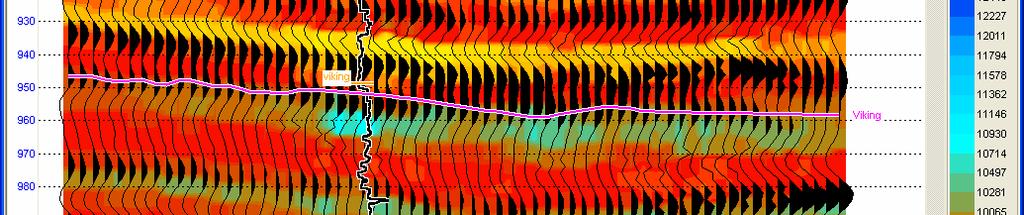
92 Application Window [2] The analysis zone is defined by the Viking and Miss tops, p, in our example. Both tops correspond with horizons, so we bound the application window by the horizons which relate to each tops, as shown. If the tops do not coincide with horizons, then use the plus option to shift the application window up/down accordingly. 92

93 2D test for your Emerge prediction: Step 5 Click OK to generate the porosity predicted volume 93

94 2D test for your Emerge prediction: Step 6 Usually the porosity volume is displayed with a normalised colour key: this needs to be altered. Firstly open the viewing parameters menu by clicking the eyeball button. 94

95 2D test for your Emerge prediction: Step 7 [1] Turn off trace data because generally speaking Emerge results are better seen as colour. [2] Select the porosity volume for the colour data. [1] [2] 95

96 2D test for your Emerge prediction: Step 8 [1] [1] Select the colour key tab. [2] Turn off Normalized Scale. [2] [3] Click Data Range. [3] 96

97 2D test for your Emerge prediction: Step 9 Enter a suitable range. 97

98 2D test for your Emerge prediction: Step 10 In this work-flow we are producing a 2D line for QC purposes. Therefore lithology colour scale is a good one to choose because you can see noise more successfully. However, for viewing your final porosity I would not recommend Lithology for the colour scale. I would suggest a white tocolour scale such as Storm because high porosity zones will stand out, since low porosity zones will be white and high porosity regions will have colour. 98

99 2D test for your Emerge prediction: Step 11 Displaying the target log as a coloured curve is another QC of the quality for your prediction [1] Select the insert tab. [2] Switch off the inserted curve by selecting none from its pull-down menu. [3] Make the inserted colour your target log. Selectyour target log as the Inserted Colour. [1] [2] [3] 99

100 2D test for your Emerge prediction: Step 12 Porosity predicted volume of inline 95. The inserted colour curve is porosity. For this QC, look for geological realism and how noisy the results are. In my opinion, the result does not look too noisy. 100

101 2D test for your Emerge prediction: Step 13 Switching to the Storm colour-key (go to colour key tab under the eye-ball), we can geologically QC the predicted volume. Our target, marked by the red square, is a channel. The shape of the feature looks like a channel furthermore we have high porosity region bounded by low porosity. Additional evidence, to suggest a channel is that the ch-top (black arrow) marks the start of the high porosity zone bound by low porosity. With all this evidence, it is reasonable to conduct the multi-attribute prediction to the full volume. We recommend that additional 2D testing of predictions with good correlation values for the validation plots should be conducted. This workflow is merely to provide a guide, which is why we are going ahead with our first test. 101

102 Applying your chosen Emerge prediction to the full volume: Step 1 Once you have found your optimum prediction after 2D testing, it is now time to Apply the prediction to the full volume. Process > Apply Emerge If processing runtime is low, it is worth running a number of predictions on the full-volume because viewing an Emerge prediction in 3D, i.e. dataslices, is a better QC than a 2D line test. In this work-flow I also show how to generate a data-slice 102

103 Applying your chosen Emerge prediction to the full volume: Step 2 [1] Keeping with the same name convention, which includes details of the prediction in the name, I also include Full because it is for the full volume. [1] [2] The full data range of the volume is inserted for the processing window [2] 103

104 Applying your chosen Emerge prediction to the full volume: Step 3 We enter the same prediction and application window as the optimum 2D test result. 104

105 Applying your chosen Emerge prediction to the full volume: Step 4 Click OK to generate the porosity volume. 105

106 Applying your chosen Emerge prediction to the full volume: Step 5 We need to visually optimize the initial porosity result. We first click the eye-ball button. 106

107 Applying your chosen Emerge prediction to the full volume: Step 6 Turn off trace data. 107

108 Applying your chosen Emerge prediction to the full volume: Step 7 [1] [1] Select the Colour key tab. [2] [] Select Storm for the colour key. [3] The software should have remembered the data-range from your 2D tests. If not, optimise the data-range from this menu. [2] [3] 108

109 Applying your chosen Emerge prediction to the full volume: Step 8 Insert the porosity log as an insert colour trace. [1] Select the insert tab. [2] Switch off inserted curve by selecting none from its pull-down menu. [3] Make the inserted colour your target log. (See page 99) [1] [2] [3] 109

110 Applying your chosen Emerge prediction to the full volume: Step 9 Full porosity volume at inline 95 with optimised visual display. 110

111 Applying your chosen Emerge prediction to the full volume: Step 10 We want to inspect the porosity volume in 3D. Therefore we need to produce a data-slice. To generate a data-slice, we select Create Data Slice from the Process pull-down menu, as shown. 111

112 Applying your chosen Emerge prediction to the full volume: Step 11 Ensure the full porosity volume is selected [1] and Amplitude is switched on [2]. [1] [3] Click Next to continue. [2] [3] 112

113 Applying your chosen Emerge prediction to the full volume: Step 12 Our goal is to produce a dataslice starting 10ms below the Ch_Top horizon with a 10ms average window. This dataslice is designed to visualise the main body of the channel. Larger extraction windows are also worth testing. Ch_Top Horizon 10ms 10ms 113

114 Applying your chosen Emerge prediction to the full volume: Step 13 [1] Use descriptive names for the dataslices so you can easily select them. [1] [2] [2] For larger volumes, you can decimate the output merely ely to save on runtime. [3] Click OK to generate the data-slice. [3] 114

115 Applying your chosen Emerge prediction to the full volume: Step 14 The red square marks the channel. Inline