Microsoft Office Excel 2010 Extra

Transcription

1 Microsoft Office Excel 2010 Extra Excel Formulas İçindekiler Microsoft Office... 1 A.Introduction About This Tutorial... 3 About this tutorial... 3 B.Formula and Function Basics Simple Formulas... 4 Introduction... 4 Challenge! Complex Formulas Introduction Challenge! Relative and Absolute Cell References Introduction Relative references Absolute references Using cell references with multiple worksheets Challenge! Functions Introduction Using functions Working with unfamiliar functions Understanding nested functions Other common functions C.Formula Tips Solving Real-Life Problems in Excel Double-Check Your Formulas Double-check your formulas Understanding Number Formats What are number formats? Using number formats correctly... 47

2 Percentage formats Date formats Number formatting tips Practice Reading Formulas Practice reading formulas Interactive: Formula Flashcards Interactive: Formula Flashcards D.Scenarios Over-Budget Items Percent-Off Sale Basketball Team: Player Statistics Movie Tickets Interactive. Pizza Party Panic Interactive:Birthday Budget Blues Using the IF Function Using CONCATENATE to Combine Names Buying a Printer: Cost Comparison E. Advanced Scenari: Create an Invoice Invoice, Part 1: Free Shipping Invoice, Part 2: Using VLOOKUP Invoice, Part 3:Fix Broken VLOOKUP Invoice, Part 4: More Shipping Options Invoice, Part 5: Data Validation Our spreadsheet Data validation in Excel Data validation with Google Sheets

3 1.About This Tutorial About this tutorial A.Introduction Welcome to our Excel Formulas tutorial! If you want to learn more about using formulas and functions in Excel or another spreadsheet application (such as Google Sheets), you've come to the right place! Whether you're new to spreadsheets or are a more advanced spreadsheet user, this tutorial is designed to show you how to use different formulas and functions to solve real-life problems. Formulas work almost exactly the same way in most spreadsheet programs, so you can work along with this tutorial even if you don't have Excel. These skills will work in Google Sheets, LibreOffice, OpenOffice, and many other spreadsheet programs. However, keep in mind that we'll be using Excel 2016 and 2013 throughout this tutorial, so you may notice some slight differences if you're using a different program. If you've never created a formula before, that's OK! This tutorial starts with the absolute basics of creating formulas and gradually works up to to some more advanced formulas. But before you begin, you'll want to have a basic understanding of how to navigate your spreadsheet program. You can review one of our other spreadsheet tutorials to learn more: Excel 2016 Excel 2013 Excel 2010 Excel 2007 Google Sheets If you already have a basic understanding of how spreadsheets work, you're ready to dive in and get started. Throughout this tutorial, you'll find a mix of written lessons, videos, and interactives that will explain the basics of formulas and guide you through real-life scenarios where you'll use formulas to solve problems! 3

4 2.Simple Formulas Introduction B.Formula and Function Basics One of the most powerful features in Excel is the ability to calculate numerical information using formulas. Just like a calculator, Excel can add, subtract, multiply, and divide. In this lesson, we'll show you how to use cell references to create simple formulas. Optional: Download our practice workbook. Watch the video below to learn how to create formulas in Excel. Mathematical operators <span id="selection-marker-1" class="redactor-selection-marker"></span> Excel uses standard operators for formulas, such as a plus sign for addition (+), a minus sign for subtraction (-), an asterisk for multiplication (*), a forward slash for division (/), and a caret (^) for exponents. All formulas in Excel must begin with an equals sign (=). This is because the cell contains, or is equal to, the formula and the value it calculates. Understanding cell references While you can create simple formulas in Excel manually (for example, =2+2 or =5*5), most of the time you will use cell addresses to create a formula. This is known as making a cell reference. Using cell references will ensure that your formulas are always accurate because you can change the value of referenced cells without having to rewrite the formula. 4

5 By combining a mathematical operator with cell references, you can create a variety of simple formulas in Excel. Formulas can also include a combination of cell references and numbers, as in the examples below: To create a formula: In our example below, we'll use a simple formula and cell references to calculate a budget. 5

6 1. Select the cell that will contain the formula. In our example, we'll select cell B3. 2. Type the equals sign (=). Notice how it appears in both the cell and the formula bar. 3. Type the cell address of the cell you want to reference first in the formula: cell B1 in our example. A blue border will appear around the referenced cell. 4. Type the mathematical operator you want to use. In our example, we'll type the addition sign (+). 6

7 5. Type the cell address of the cell you want to reference second in the formula: cell B2 in our example. A red border will appear around the referenced cell. 6. Press Enter on your keyboard. The formula will be calculated, and the value will be displayed in the cell. If the result of a formula is too large to be displayed in a cell, it may appear as pound signs (#######) instead of a value. This means the column is not wide enough to display the cell content. Simply increase the column width to show the cell content. Modifying values with cell references The true advantage of cell references is that they allow you to update data in your worksheet without having to rewrite formulas. In the example below, we've modified the value of cell B1 from $1,200 to $1,800. The formula in B3 will automatically recalculate and display the new value in cell B3. 7

8 Excel will not always tell you if your formula contains an error, so it's up to you to check all of your formulas. To learn how to do this, you can read the Double-Check Your Formulas lesson from our Excel Formulas tutorial. To create a formula using the point-and-click method: Rather than typing cell addresses manually, you can point and click on the cells you want to include in your formula. This method can save a lot of time and effort when creating formulas. In our example below, we'll create a formula to calculate the cost of ordering several boxes of plastic silverware. 1. Select the cell that will contain the formula. In our example, we'll select cell D3. 2. Type the equals sign (=). 8

9 3. Select the cell you want to reference first in the formula: cell B3 in our example. The cell address will appear in the formula, and a dashed blue line will appear around the referenced cell. 4. Type the mathematical operator you want to use. In our example, we'll type the multiplication sign (*). 5. Select the cell you want to reference second in the formula: cell C3 in our example. The cell address will appear in the formula, and a dashed red line will appear around the referenced cell. 6. Press Enter on your keyboard. The formula will be calculated, and the value will be displayed in the cell. 9

10 Formulas can also be copied to adjacent cells with the fill handle, which can save a lot of time and effort if you need to perform the same calculation multiple times in a worksheet. Review our lesson on Relative and Absolute Cell References to learn more. 10

11 To edit a formula: Sometimes you may want to modify an existing formula. In the example below, we've entered an incorrect cell address in our formula, so we'll need to correct it. 1. Select the cell containing the formula you want to edit. In our example, we'll select cell B3. 2. Click the formula bar to edit the formula. You can also double-click the cell to view and edit the formula directly within the cell. 3. A border will appear around any referenced cells. In our example, we'll change the second part of the formula to reference cell B2 instead of cell C2. 11

12 4. When you're finished, press Enter on your keyboard or click the checkmark in the formula bar. 5. The formula will be updated, and the new value will be displayed in the cell. If you change your mind, you can press the Esc key on your keyboard to avoid accidentally making changes to your formula. To show all of the formulas in a spreadsheet, you can hold the Ctrl key and press ` (grave accent). The grave accent key is usually located in the top-left corner of the keyboard. You can press Ctrl+` again to switch back to the normal view. 12

13 Challenge! 1. Open an existing Excel workbook. If you want, you can use our practice workbook. 2. Create a simple addition formula using cell references. If you are using the example, create the formula in cell B4 to calculate the total budget. 3. Try modifying the value of a cell referenced in a formula. If you are using the example, change the value of cell B2 to $2,000. Notice how the formula in cell B4 recalculates the total. 4. Try using the point-and-click method to create a formula. If you are using the example, create a formula in cell G5 that multiplies the cost of napkins by the quantity needed to calculate the total cost. 5. Edit a formula using the formula bar. If you are using the example, edit the formula in cell B9 to change the division sign (/) to a minus sign (-). 13

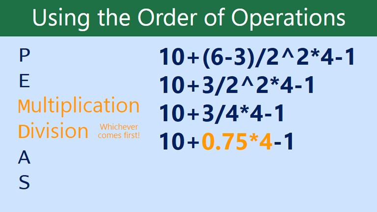
14 3.Complex Formulas Introduction A simple formula is a mathematical expression with one operator, such as 7+9. A complex formula has more than one mathematical operator, such as 5+2*8. When there is more than one operation in a formula, the order of operations tells your spreadsheet which operation to calculate first. In order to use complex formulas, you will need to understand the order of operations. Optional: Download our example file for this lesson. Watch the video below to learn more about complex formulas. The order of operations All spreadsheet programs calculate formulas based on the following order of operations: 1. Operations enclosed in parentheses 2. Exponential calculations (3^2, for example) 3. Multiplication and division, whichever comes first 4. Addition and subtraction, whichever comes first A mnemonic that can help you remember the order is PEMDAS, or Please Excuse My Dear Aunt Sally. Click the arrows in the slideshow below to learn more about how the order of operations is used to calculate complex formulas. While this formula may look really complicated, we can use the order of operations step by step to find the right answer. 14

15 15

16 16

17 Using parentheses within a formula can be very important. Because of the order of operations, it can completely change an answer. Let's try the same problem from above, but this time we'll add parentheses to the last part. Creating complex formulas In the example below, we'll demonstrate a complex formula using the order of operations. Here, we want to calculate the cost of sales tax for a catering invoice. To do this, we'll write our formula as =(D2+D3)*0.075 in cell D4. This formula will add the prices of our items together and then multiply that value by the 7.5% tax rate (which is written as 0.075) to calculate the cost of sales tax. 17

18 The spreadsheet then follows the order of operations and first adds the values inside the parentheses: ( ) = $ Then it multiplies that value by the tax rate: $84.75* The result will show that the sales tax is $6.36. It is especially important to enter complex formulas with the correct order of operations. Otherwise, the spreadsheet will not calculate the results accurately. In our example, if the parentheses are not included, the multiplication is calculated first and the result is incorrect. Parentheses are the best way to define which calculations will be performed first in a formula. 18

19 To create a complex formula using the order of operations: In our example below, we will use cell references along with numerical values to create a complex formula that will calculate the total cost for a catering invoice. The formula will calculate the cost for each menu item and add those values together. 1. Select the cell that will contain the formula. In our example, we'll select cell C4. 2. Enter your formula. In our example, we'll type =B2*C2+B3*C3. This formula will follow the order of operations, first performing multiplication: 2.29*20 = and 3.49*35 = Then it will add those values together to calculate the total: Double-check your formula for accuracy, then press Enter on your keyboard. The formula will calculate and display the result. In our example, the result shows that the total cost for the order is $

20 You can add parentheses to any equation to make it easier to read. While it won't change the result of the formula in this example, we could enclose the multiplication operations within parentheses to clarify that they will be calculated before the addition. Your spreadsheet will not always tell you if your formula contains an error, so it's up to you to check all of your formulas. To learn how to do this, check out the Double-Check Your Formulas lesson. Challenge! 1. Open an existing Excel workbook. If you want, you can use the example file for this lesson. 2. Create a complex formula that will perform addition before multiplication. If you are using the example, create a formula in cell D6 that first adds the values of cells D3, D4, and D5 and then multiplies their total by Hint: You'll need to think about the order of operations for this to work correctly. 20

21 4.Relative and Absolute Cell References Introduction There are two types of cell references: relative and absolute. Relative and absolute references behave differently when copied and filled to other cells. Relative references change when a formula is copied to another cell. Absolute references, on the other hand, remain constant no matter where they are copied. Optional: Download our example file for this lesson. Watch the video below to learn more about cell references. Relative references By default, all cell references are relative references. When copied across multiple cells, they change based on the relative position of rows and columns. For example, if you copy the formula =A1+B1 from row 1 to row 2, the formula will become =A2+B2. Relative references are especially convenient whenever you need to repeat the same calculation across multiple rows or columns. To create and copy a formula using relative references: In the following example, we want to create a formula that will multiply each item's price by the quantity. Rather than create a new formula for each row, we can create a single formula in cell D2 and then copy it to the other rows. We'll use relative references so the formula correctly calculates the total for each item. 1. Select the cell that will contain the formula. In our example, we'll select cell D2. 21

22 2. Enter the formula to calculate the desired value. In our example, we'll type =B2*C2. 3. Press Enter on your keyboard. The formula will be calculated, and the result will be displayed in the cell. 4. Locate the fill handle in the lower-right corner of the desired cell. In our example, we'll locate the fill handle for cell D2. 22

23 5. Click, hold, and drag the fill handle over the cells you wish to fill. In our example, we'll select cells D3:D Release the mouse. The formula will be copied to the selected cells with relative references and the values will be calculated in each cell. 23

24 You can double-click the filled cells to check their formulas for accuracy. The relative cell references should be different for each cell, depending on its row. Absolute references There may be times when you do not want a cell reference to change when filling cells. Unlike relative references, absolute references do not change when copied or filled. You can use an absolute reference to keep a row and/or column constant. An absolute reference is designated in a formula by the addition of a dollar sign ($). It can precede the column reference, the row reference, or both. You will usually use the $A$2 format when creating formulas that contain absolute references. The other two formats are used much less frequently. When writing a formula in Microsoft Excel, you can press the F4 key on your keyboard to switch between relative and absolute cell references. This is an easy way to quickly insert an absolute reference. 24

25 To create and copy a formula using absolute references: In our example, we'll use the 7.5% sales tax rate in cell E1 to calculate the sales tax for all items in column D. We'll need to use the absolute cell reference $E$1 in our formula. Because each formula is using the same tax rate, we want that reference to remain constant when the formula is copied and filled to other cells in column D. 1. Select the cell that will contain the formula. In our example, we'll select cell D3. 2. Enter the formula to calculate the desired value. In our example, we'll type =(B3*C3)*$E$1. 25

26 3. Press Enter on your keyboard. The formula will calculate, and the result will display in the cell. 4. Locate the fill handle in the lower-right corner of the desired cell. In our example, we'll locate the fill handle for cell D3. 26

27 5. Click, hold, and drag the fill handle over the cells you wish to fill, cells D4:D13 in our example. 6. Release the mouse. The formula will be copied to the selected cells with an absolute reference, and the values will be calculated in each cell. 27

28 You can double-click the filled cells to check their formulas for accuracy. The absolute reference should be the same for each cell, while the other references are relative to the cell's row. Be sure to include the dollar sign ($) whenever you're making an absolute reference across multiple cells. The dollar signs were omitted in the example below. This caused the 28

29 spreadsheet to interpret it as a relative reference, producing an incorrect result when copied to other cells. Using cell references with multiple worksheets Most spreadsheet programs allow you to refer to any cell on any worksheet, which can be especially helpful if you want to reference a specific value from one worksheet to another. To do this, you'll simply need to begin the cell reference with the worksheet name followed by an exclamation point (!). For example, if you wanted to reference cell A1 on Sheet1, its cell reference would be Sheet1!A1. Note that if a worksheet name contains a space, you will need to include single quotation marks (' ') around the name. For example, if you wanted to reference cell A1 on a worksheet named July Budget, its cell reference would be 'July Budget'!A1. To reference cells across worksheets: In our example below, we'll refer to a cell with a calculated value between two worksheets. This will allow us to use the exact same value on two different worksheets without rewriting the formula or copying data between worksheets. 1. Locate the cell you wish to reference, and note its worksheet. In our example, we want to reference cell E14 on the Menu Order worksheet. 29

30 2. Navigate to the desired worksheet. In our example, we'll select the Catering Invoice worksheet. 3. The selected worksheet will appear. 4. Locate and select the cell where you want the value to appear. In our example, we'll select cell B2. 30

31 5. Type the equals sign (=), the sheet name followed by an exclamation point (!), and the cell address. In our example, we'll type ='Menu Order'!E Press Enter on your keyboard. The value of the referenced cell will appear. If the value of cell E14 changes on the Menu Order worksheet, it will be updated automatically on the Catering Invoice worksheet. 31

32 If you rename your worksheet at a later point, the cell reference will be updated automatically to reflect the new worksheet name. Challenge! 1. Open an existing Excel workbook. If you want, you can use the example file for this lesson. 2. Create a formula that uses a relative reference. If you are using the example, use the fill handle to fill in the formula in cells E4 through E14. Double-click a cell to see the copied formula and the relative cell references. 3. Create a formula that uses an absolute reference. If you are using the example, correct the formula in cell D4 to refer only to the tax rate in cell E2 as an absolute reference, then use the fill handle to fill the formula from cells D4 to D Try referencing a cell across worksheets. If you are using the example, create a cell reference in cell B3 on the Catering Invoice worksheet for cell E15 on the Menu Order worksheet. 32

33 5.Functions Introduction A function is a predefined formula that performs calculations using specific values in a particular order. All spreadsheet programs include common functions that can be used for quickly finding the sum, average, count, maximum value, and minimum value for a range of cells. In order to use functions correctly, you'll need to understand the different parts of a function and how to create arguments to calculate values and cell references. Watch the video below to learn more about using functions in Excel. The parts of a function In order to work correctly, a function must be written a specific way, which is called the syntax. The basic syntax for a function is an equals sign (=), the function name (SUM, for example), and one or more arguments. Arguments contain the information you want to calculate. The function in the example below would add the values of the cell range A1:A20. Working with arguments Arguments can refer to both individual cells and cell ranges and must be enclosed within parentheses. You can include one argument or multiple arguments, depending on the syntax required for the function. For example, the function =AVERAGE(B1:B9) would calculate the average of the values in the cell range B1:B9. This function contains only one argument. 33

34 Multiple arguments must be separated by a comma. For example, the function =SUM(A1:A3, C1:C2, E2) will add the values of all cells in the three arguments. Using functions There are a variety of functions. Here are some of the most common functions you'll use: SUM: This function adds all the values of the cells in the argument. AVERAGE: This function determines the average of the values included in the argument. It calculates the sum of the cells and then divides that value by the number of cells in the argument. COUNT: This function counts the number of cells with numerical data in the argument. This function is useful for quickly counting items in a cell range. MAX: This function determines the highest cell value included in the argument. 34

35 MIN: This function determines the lowest cell value included in the argument. To use a function: In our example below, we'll use a basic function to calculate the average price per unit for a list of recently ordered items using the AVERAGE function. 1. Select the cell that will contain the function. In our example, we'll select cell C Type the equals sign (=) and enter the desired function name. In our example, we'll type =AVERAGE. 35

36 3. Enter the cell range for the argument inside parentheses. In our example, we'll type (C3:C10). This formula will add the values of cells C3:C10 and then divide that value by the total number of cells in the range to determine the average. 36

37 4. Press Enter on your keyboard. The function will be calculated, and the result will appear in the cell. In our example, the average price per unit of items ordered was $ Your spreadsheet will not always tell you if your function contains an error, so it's up to you to check all of your functions. To learn how to do this, check out the Double-Check Your Formulas lesson. Working with unfamiliar functions If you want to learn how a function works, you can start typing that function in a blank cell to see what it does. You can then type an open parenthesis to see what kind of arguments it needs. 37

38 Understanding nested functions Whenever a formula contains a function, the function is generally calculated before any other operators, like multiplication and division. That's because the formula treats the entire function as a single value before it can use that value in the formula, it needs to run the function. For example, in the formula below, the SUM function will be calculated before division: Let's take a look at a more complicated example that uses multiple functions: =WORKDAY(TODAY(),3) Here, we have two different functions working together: the WORKDAY function and the TODAY function. These are known as nested functions, since one function is placed, or nested, within the arguments of another. As a rule, the nested function is always calculated first, just like parentheses are performed first in the order of operations. In this example, the TODAY function will be calculated first, since it's nested within the WORKDAY function. Other common functions There are many other functions you can use to quickly calculate different things with your data. Learning how to use other functions will allow you to solve complex problems with your spreadsheets, and we'll be talking more about them throughout this tutorial. You can also check out our articles below to learn about specific functions: 38

39 How to Use Excel's VLOOKUP Function How to Count Cells with COUNTA Use SUMPRODUCT to Calculate Weighted Averages CONCATENATE: Excel's Duct Tape Use the PROPER Function to Capitalize Names in Excel 39

40 6.Solving Real-Life Problems in Excel Solving real-life problems in Excel C.Formula Tips Excel can be used to solve all kinds of real-life problems. But how do you turn those problems into formulas that Excel can understand? All it takes is a little bit of planning (and some basic math). To learn more, check out the video below! 40

41 7.Double-Check Your Formulas Double-check your formulas One of the most powerful features of Excel is the ability to create formulas. You can use formulas to calculate new values, analyze data, and much more. But formulas also have a downside: If you make even a small mistake when typing a formula, it can give an incorrect result. To make matters worse, your spreadsheet will not always tell you if a formula is wrong. It will usually just go ahead and run the calculations and give you the wrong answer. It's up to you to double-check your formulas whenever you create them. We've put together a list of tips you can use to help check formulas for accuracy. These tips won't help you solve every problem you encounter, but they should provide you with the tools to identify many common errors. Check the references Most formulas use at least one cell reference. When you double-click a formula, it will highlight all of the referenced cells. You can then double-check each one to make sure they are correct. Look for mix-ups A common mistake is to use the correct cell references, but in the wrong order. For example, if you want to subtract C2 from C3, the formula should be =C3-C2, not =C2-C3. Break it up If a formula is too complicated to check, try breaking it up into several smaller formulas. This way, you can check each formula for accuracy, and if there are any problems you will know exactly where they are. 41

42 Ballpark it You can use your own experience, critical-thinking skills, and common sense to estimate what the answer should be. If Excel gives you a much larger or smaller value than expected, there may be a problem with your formula (or with the values in the cells). For example, if you are calculating the total price of 8 items that are 98 cents each, the answer should be slightly less than $8. In the example below, the formula calculated the answer as $784.00, which is incorrect. That's because the price in A2 was entered as 98, and it should have been As you can see, even the smallest details can make a huge difference. Note that this tip does not always work. In some cases, the wrong answer may be fairly close to the correct answer. However, in many situations it can help you quickly catch a problem in your formula. Check the arguments If you're using a function, make sure each required argument is included. A small dialog box should appear as you're typing the function to let you know what arguments are needed. This can be especially useful when you're trying to fix a function that's not working correctly. For example, let's look at the function below: 42

43 In the example above, the NETWORKDAYS function is returning an error. If we enter the NETWORKDAYS function into a new cell, the reason becomes clear: The NETWORKDAYS function requires at least two arguments a start date and an end date. Our original function only has one argument, so we'll edit our function to include both arguments: Now our function is working correctly! Walk through the order of operations Remember the order of operations from math class? If not (or if you want a refresher), you can check out our Complex Formulas lesson. Your spreadsheet will always use this ordering, which means it doesn't just calculate a formula from left to right. In the example below, the multiplication is calculated first, which isn't what we wanted. We could fix this formula by enclosing D2+D3 in parentheses. 43

44 Switch to formula view If you have a lot of formulas and functions in your spreadsheet, you may want to switch to formula view to see all of them at the same time. Just hold the Ctrl key and press ` (grave accent). The grave accent key is usually located in the upper-left corner of the keyboard. Press Ctrl+` again to switch back to normal view. Remember, it takes a lot of practice to master writing formulas. Even the most experienced spreadsheet users encounter formula errors. If your formula doesn't work or produces an incorrect value, don't panic! More often than not, there's probably a simple reason your formula resulted in an error once you find it, you'll be able to get your formula working correctly. 44

45 8.Understanding Number Formats What are number formats? Whenever you're working with a spreadsheet, it's a good idea to use appropriate number formats for your data. Number formats tell your spreadsheet exactly what type of data you're using, such as percentages (%), currency ($), times, dates, and so on. For example, take a look at this spreadsheet, which uses a variety of number formats: Why use number formats? Number formats don't just make your spreadsheet easier to read they also make it easier to use. When you apply a number format, you're telling your spreadsheet exactly what kinds of values are stored in a cell. For example, the date format tells the spreadsheet that you're entering specific calendar dates. This allows the spreadsheet to better understand your data, which can help ensure that your data remains consistent and that your formulas are calculated correctly. If you don't need to use a specific number format, the spreadsheet will usually apply the general number format by default. However, the general format may apply some small formatting changes to your data. Applying number formats Just like other types of formatting, such as changing the font color, you'll apply number formats by selecting cells and then choosing the desired formatting option. Every spreadsheet program allows you to add number formatting, but the process will vary depending on which application you're using: 45

46 For Microsoft Excel , go to the Home tab, click the Number Format drop-down menu in the Number group, and select the desired format. You can also click one of the quick number-formatting commands below the drop-down menu. For Excel 2003 and earlier, go to Format > Cells. For Google Sheets, click the More Formats button near the left side of the toolbar this button will look like the numbers 123. To the left of the command, you can also click the Currency or Percent commands to quickly apply those formats. For most versions of Microsoft Excel, you can also select the desired cells and press Ctrl+1 on your keyboard to access more number-formatting options. In this example, we've applied the Currency number format, which adds currency symbols ($) and displays two decimal places for any numerical values. 46

47 If you select any cells with number formatting, you can see the actual value of the cell in the formula bar. The spreadsheet will use this value for formulas and other calculations. Using number formats correctly There's more to number formatting than selecting cells and applying a format. Spreadsheets can actually apply a lot of number formatting automatically based on the way you enter data. This means you'll need to enter data in a way the program can understand, and then ensure that those cells are using the proper number format. For example, the image below shows how to use number formats correctly for dates, percentages, and times: 47

48 Now that you know more about how number formats work, we'll look at a few different number formats in action. Percentage formats One of the most helpful number formats is the percentage (%) format. It displays values as percentages, such as 20% or 55%. This is especially helpful when calculating things like the cost of sales tax or a tip. When you type a percent sign (%) after a number, the percentage number format will be be applied to that cell automatically. As you may remember from math class, a percentage can also be written as a decimal. So 15% is the same thing as 0.15, 7.5% is 0.075, 20% is 0.20, 55% is 0.55, and so on. You can review this lesson from our Math tutorial to learn more about converting percentages to decimals. There are many times when percentage formatting will be useful. For example, in the images below, notice how the sales tax rate is formatted differently for each spreadsheet (5, 5%, and 0.05): 48

49 As you can see, the calculation in the spreadsheet on the left didn't work correctly. Without the percentage number format, our spreadsheet thinks we want to multiply $22.50 by 5, not 5%. And while the spreadsheet on the right still works without percentage formatting, the spreadsheet in the middle is easier to read. Date formats Whenever you're working with dates, you'll want to use a date format to tell the spreadsheet that you're referring to specific calendar dates, such as July 15, Date formats also allow you to work with a powerful set of date functions that use time and date information to calculate an answer. Spreadsheets don't understand information the same way a person would. For instance, if you type October into a cell, the spreadsheet won't know you're entering a date so it will treat it like any other text. Instead, when you enter a date, you'll need to use a specific format your spreadsheet understands, such as month/day/year (or day/month/year depending on which country you're in). In the example below, we'll type 10/12/2014 for October 12, Our spreadsheet will then automatically apply the date number format for the cell. Now that we have our date correctly formatted, we can do lots of different things with this data. For example, we could use the fill handle to continue the dates through the column, so a different day appears in each cell: 49

50 If the date formatting isn't applied automatically, it means the spreadsheet did not understand the data you entered. In the example below, we've typed March 15th. The spreadsheet did not understand that we were referring to a date, so this cell is still using the general number format. 50

51 On the other hand, if we type March 15 (without the "th"), the spreadsheet will recognize it as a date. Since it doesn't include a year, the spreadsheet will automatically add the current year so the date will have all of the necessary information. We could also type the date several other ways, such as 3/15, 3/15/2014, or March , and the spreadsheet would still recognize it as a date. Try entering the dates below into a spreadsheet and see if the date format is applied automatically: 10/12 October October 12 October /12/2014 October 12, October 12th Other date-formatting options Some programs have more date-formatting options, which can change the way dates appear in your spreadsheet. Again, this process this may vary slightly based on the spreadsheet program you're using. To access these options in Excel , select the Number Format dropdown menu and choose More Number Formats. 51

52 A dialog box will appear. From here, you can choose the desired date-formatting option. 52

53 As you can see in the formula bar, a custom date format doesn't change the actual date in our cell it just changes the way it's displayed. Number formatting tips Here are a few tips for getting the best results with number formatting: Apply number formatting to an entire column: If you're planning to use one column for a certain type of data, like dates or percentages, you may find it easiest to select the entire column by clicking the column letter and then applying the desired number formatting. This way, any data you add to this column in the future will already have the correct number format. Note that the header row usually won't be affected by number formatting. 53

54 Double-check your values after applying number formatting: If you apply number formatting to existing data, you may have unexpected results. For example, applying percentage (%) formatting to a cell with a value of 5 will give you 500%, not 5%. In this case, you'd need to retype the values correctly in each cell. 54

55 If you reference a cell with number formatting in a formula, the spreadsheet may automatically apply the same number formatting to the new cell. For example, if you use a value with currency formatting in a formula, the calculated value will also use the currency number format. If you want your data to appear exactly as entered, you'll need to use the text number format. This format is especially good for numbers you don't want to perform calculations with, such as phone numbers, zip codes, or numbers that begin with 0: for example, "02415". For best results, you may want to apply the text number format before entering data in those cells. 55

56 9.Practice Reading Formulas Practice reading formulas If you ever use a spreadsheet that was created by someone else, you'll also need to read the formulas in that spreadsheet. Reading a formula written by someone else can be tricky it may not be immediately obvious why someone chose a certain formula, or how it's working. If you're struggling to read a formula, don't panic! Many formulas are actually less complicated than they appear, but it may take some time and effort to figure out how they work. With that in mind, we've put together a list of tips to help you read formulas. You may also find the tips in our Double-Check Your Formulas lesson to be helpful. Determine which cells contain formulas It's important to remember that any cell can contain a formula, and it won't always be obvious which cells contain them. You may want to get in the habit of checking the formula bar to see if the currently selected cell contains a formula. You can also double-click a cell that contains a formula to see what cells it's referencing. You can also switch to formula view, which will display all of the formulas in the spreadsheet. This can help you understand how the spreadsheet is put together and where the formulas are stored. Just hold the Ctrl key and press ` (grave accent). The grave accent key is usually located in the upper-left corner of the keyboard. Press Ctrl+` again to switch back to normal view. 56

57 Try to understand what the formula is doing Whenever you read a formula, you'll need to think about why that formula was used, and what it's doing in the spreadsheet. The same is true for functions. For example, let's take a look at this spreadsheet a running log our friend Sophie created: It looks like Sophie didn't label the calculated value in cell B8. However, if we take a look at the formula we can see that she used the AVERAGE function to find the average of the values in cell range B3:B7. Based on the data in column B, we can reasonably guess that she used this formula to find the average distance for these different runs. 57

58 Think about the order of operations Remember the order of operations from math class? If not (or if you want a refresher), you can check out our Complex Formulas lesson. Your spreadsheet will always use this ordering, which means it doesn't just calculate a formula from left to right. If you're not sure how a formula is working, try walking through the order of operations to figure out how it's calculating a value. It's also important to remember that whenever a formula contains a function, the function is generally calculated before any other operators, like multiplication and division. For example, in the formula below, the SUM function will be calculated before division: If one function is nested inside another function, the innermost function will be calculated first. For example, in the formula =WORKDAY(TODAY(),3), the TODAY function will be calculated first. You can review our lesson on Functions to learn more about how functions work within formulas. 58

59 10.Interactive: Formula Flashcards Interactive: Formula Flashcards Let's briefly review what we have learned in the past few lessons. Then, you'll answer a few questions to test your knowledge. Simple Formulas Simple formulas combine relative cell references and mathematical operators to perform helpful calculations. Complex Formulas Like simple formulas, complex formulas combine cell references and mathematical operators. However, in complex formulas, we usually perform more than one mathematical operation. The order of operations helps us to determine which operation to perform first. Functions A function is a predefined formula that performs calculations using specific values in a particular order. The first step, however, is determining which function to use. To review the different types of functions, you can check out our Functions lesson. The second step to using a function is determining the correct arguments. Arguments determine which cells are analyzed by a function. Now that you know the basics of formulas and functions, you're ready to learn some more advanced Excel formulas! 59

60 11.Over-Budget Items Our spreadsheet D.Scenarios Once you've downloaded our spreadsheet, open the file in Excel or another spreadsheet application. As you can see, our coworker Carter has given us a pretty simple budget: Each category is on a separate row, and there are columns for the projected costs and actual costs. What are we trying to find out? Before we try to create our formulas, let's think about the question we're trying to answer: "Which expenses are over budget?" How do we know if something is over budget? In this example, we can compare the projected and actual costs. If the actual cost is higher than the projected cost, then it is over budget. Writing the formula Now we just need to decide how to represent this idea in a formula. One way to compare two values is to subtract one from the other. In our example, we could simply subtract the actual cost from the projected cost. If the result is negative, then we know that category is over budget. In our example, we expected to spend $14,000 on Facilities, and we actually spent $15,000. If we subtract $15,000 from $14,000, the result would be -$1,000 (negative $1,000). We could also say this category is $1,000 over budget. Our projected expenses are in column B, and our actual expenses are in column C. So for the first category, the formula to compare these values would be: =B2-C2 Let s type this formula into cell D2: 60

61 Next, we can just drag the fill handle down to add the formula to the other cells in the column: Now we can see that several of the categories have negative values, which means they are over budget. Carter is right: Although this spreadsheet gives us an answer, it isn't very easy to read. There are a few different ways we could make the over-budget items more noticeable. For example: We could filter the data to only show rows that have a negative result. We could add conditional formatting to make the negative cells red. We could select the data and create a chart, which will make the data more visual. All of these solutions will work there isn't a right or wrong answer. You may want to experiment with different methods to see which one you think is the clearest. In our example, we ll add conditional formatting. 61

62 First, make sure the values in column D are selected. Next, we'll need to create a conditional formatting rule that looks for cells containing a value less than zero. The process will vary depending on which spreadsheet program you're using: For Excel : From the Home tab, select Conditional Formatting > Highlight Cells Rules > Less Than. For Excel 2003 and earlier: Go to Format > Conditional Formatting. For Google Sheets: Go to Format > Conditional Formatting. Make sure the rule is set to "Less than" and that the value is set to "0" (to look for cells that are less than zero), and choose a formatting option that will stand out. In this case, a red background with red text is a good choice. 62

63 If you're using Microsoft Excel, another option would be to apply a Currency number format that will make the negative numbers appear as red text. That's it! Now we can easily see at a glance which items are over budget. 63

64 12.Percent-Off Sale Our spreadsheet Once you've downloaded our spreadsheet, open the file in Excel or another spreadsheet application. Here, we have two main columns: one for the item name, and another for the item price. There's also a formula in cell B5 that calculates the original total cost of the items: =SUM(B2:B4) What are we trying to figure out? Let's think about the problem we're trying to solve. We want to know the total cost after the discount. A discount is a percentage of the original price. In this example, the discount is 15% of the original total. To make this problem easier to solve with a spreadsheet, we'll break it down into two steps: 1. Find the discount, which is 15% of $ Subtract that value from the original total to find the final cost. Step 1: Find the discount We know that we need a formula that will calculate 15% of $ Whenever you see the phrase "of something" in a percentage problem, it's a hint that you need to multiply. So we'll need to multiply $78.77 by 15% to find the discount. When you're using percentages within formulas, you'll want to write them as decimals. Excellent! Now that we know how to write 15% as a decimal, we're ready to write our formula: =B5*0.15 We'll type this formula in cell B6 and then press Enter: 64

65 And here's our answer: The discount is $ Step 2: Subtract the discount from the original total Now that we've calculated our discount, we'll subtract that value from the original total. Here's our formula: =B5-B6 We'll type this formula in cell B7 and press Enter: The final price after the discount will be $

66 Bonus Section In the example above, we found the discount and then subtracted that from the original total. To make this simpler, we broke the problem down into two smaller steps. However, if you're comfortable working with percentage problems, we could have found the same answer with only one formula. Can you figure out which formula we could have used instead? Here's a hint: Because we know we'll get 15% off, you could also say the final cost would be 85% of the original total. 66

67 13.Basketball Team: Player Statistics Our spreadsheet Once you've downloaded our spreadsheet, open the file in Excel or another spreadsheet application. You may want to take a moment to see how the data is organized. As you can see, there is a different row for each of the players and different columns for the number of points they scored in each game. What are we trying to figure out? Before we write our formulas, let's think about the problem we're trying to solve. Our friend wants to find out which player scored the most points total over these five games. Writing the formula Now that we know what function to use, we'll start by calculating the total points scored for Tonya in row 2. 67

68 Before we write the formula, we'll need to decide what cell range to include in the argument. Now we're ready to write our formula. Go to the next page to see our formula in action! Writing the formula Now that we know what function and cell range to use, we're ready to enter our formula, =SUM(B2:F2), in cell G2: 68

69 It looks like Tonya scored 51 points total. Next, we'll drag the fill handle down to add this formula for the other players. There we go! It looks like Bella scored the most points overall. However, we could take it a bit further to make our data really stand out. For example, we could: Apply conditional formatting to highlight the highest values Create a chart to visually compare the results Sort the results There's really no right answer in this case the most important thing is to make your data clear and easier to understand. In this example, it might be especially helpful to sort the data by the total points scored from highest to lowest this will show who the top scorer is and make it easier to rank the other players on the team. Sorting works a bit differently, depending on which spreadsheet program you're using: For Excel : Select column G, then click the Descending Sort (Z-A) command on the Data tab. For Excel 2003 and earlier: Select column G, then click Data > Sort > Descending. For Google Sheets: Select column G, then click Data > Sort sheet by column G > Descending. 69

70 OK, now it's really easy to read our results! We can tell at a glance that Bella is the highest scorer, and we can also rank the other players. Highest-scoring game for each player Now we'll need to answer this question: How many points did each of the players score in their best-scoring game? Now that we know what function to use, we'll start by finding the highest-scoring game for Bella in row 2. 70

71 Before we write our formula, we'll need to decide what cell range to include in the argument. Go to the next page to see our formula in action! Highest-scoring game Now that we know what function and cell range to use, we'll type our formula, =MAX(B2:F2), in cell H2 and then use the fill handle to add it to the other cells in column H. Now we can easily see how many points each of the players scored in their highest-scoring game! 71

72 14.Movie Tickets Our spreadsheet Once you've downloaded our spreadsheet, open the file in Excel or another spreadsheet application. We'll just need to enter a few different values to get started. Our friend Darien told us that a ticket costs $11.75, so we'll enter that in cell B1. He'll need 4 tickets (one for himself and three for his friends), so we'll enter 4 into cell B2. Finally, Darien said he didn't want to spend more than $50.00, so we'll enter that in cell B3. How can we solve this problem? Darien wants to know how much money he'll have after buying the tickets. To simplify the problem, we're going to break it down into two steps: 1. Figure out how much the tickets will cost. 2. Subtract that amount from the total budget to find our answer. Writing the formulas Let's start by calculating the cost of the tickets. To find the answer, we'll multiply the cost of the tickets by the number of tickets needed. Those values are stored in cells B1 and B2. So here's our formula: =B1*B2 We'll type this formula into cell B4: 72

73 OK, the tickets will cost $ Now, we'll subtract that value from the total budget in cell B3. Here's our formula: =B3-B4 We'll type this formula into cell B5: So if Darien buys 4 regularly priced tickets, he'll have $3.00 left over for popcorn and drinks. Since we used cell references to write our formulas, we can simply change the ticket cost in cell B1 from $11.75 to $7.25 our formulas will then recalculate automatically. OK, Darien will have $21.00 left over if he chooses to go to the matinee showing of the movie! Let's send this back to him. Bonus Section In the example above, we used two different formulas to make the problem easier to solve. But if you're already familiar with the order of operations, you might have realized that we could have written it as one formula. In the interactive below, see if you can select a formula that would do this. This formula gives us the same answer as the example above: $ As you may remember from the lesson on Complex Formulas, spreadsheets use the order of operations to determine which operations to perform first in a formula. Because multiplication comes before subtraction, this formula will first multiply the values in cells B1 and B2 and then subtract that value from the budget total in cell B3. 73

74 Of course, it's up to you to determine how you want to solve problems in a spreadsheet. However, as you become more confident with using the order of operations, you may find it easier to write only one formula to solve complex problems, as in the example above. 74

75 15.Interactive. Pizza Party Panic 75

76 16.Interactive:Birthday Budget Blues 76

77 17.Using the IF Function Our spreadsheet Once you've downloaded our spreadsheet, open the file in Excel or another spreadsheet application. As you can see, our coworker Jordan has already added a ton of information there are several different columns, and each row contains the contact information for one person, along with the amount of money that person donated. How can we solve this problem quickly? So if a person donated at least $50, we need to write the words Free Gift in that donor's row. We could go through each row, look at the value, and then write Free Gift if the value is at least $50. But there are a lot of people on the spreadsheet, so it could be really time consuming to do this manually. What we really need is way to make our spreadsheet do this automatically. While you might never have used it before, the IF function can simplify these kinds of problems. The IF function can look at a value in a cell to see if it meets a basic condition (in our example, if the value is greater than or equal to 50). Then it can then add text to an empty cell. Here, we can use the IF function to look at each person's donation, then add the words Free Gift if they donated at least $50. Basically, the IF function can do the same thing we were planning to do, only it can do it much faster. Prepare the spreadsheet If you've never used the IF function before, don't worry it's not complicated, although the syntax is a bit different from other formulas you may have used. Before you get started, it's best to decide where the results from the function will go. In our case, we'll go ahead and insert a new column to the right of column G. 77

78 Writing the function Now that we have our new column, we'll start building our formula. We'll need to have a formula on each row, so we'll start by typing the formula in cell H2. As with any formula, you'll start with an equals sign (=). Then type the function name, followed by an open parenthesis. So far, it should look like this: =IF( Now, we'll add our arguments. The arguments will tell the IF function what to look for and what to write in the cell depending on the outcome. The first argument sets up the condition we want to test. For this formula, we want to know if the value in cell G2 is greater than or equal to 50. We'll use some mathematical operators ( > for greater than and = for equals ) to write the condition: =IF(G2>=50 The next argument will tell the function what to write if the condition is true (that is, if the value is greater than or equal to 50). This means the person will be getting a free gift, so we'll have it write Free Gift. Because this argument is text, we'll need to put it in double quotes (" "). And, as with any function, we'll need to use a comma to separate each argument: =IF(G2>=50, "Free Gift" The final argument will tell the function what to write if the condition is false. This means the person won't get a free gift. We could make the function write something like None or No, but in this case we actually just want the cell to remain blank. To do this, we'll just type double quotes ("") with no text inside. This is also our last argument, so go ahead and close the parentheses: =IF(G2>=50, "Free Gift", "") OK, you're done! When you press Enter, the words Free Gift should appear in the cell. 78

79 Now we can just drag the fill handle down to add the formula to the other cells in column H: Excellent our function is working perfectly! If we wanted to go a step further, we might sort or filter the results to show only those donors who earned the free gift. For now, it looks like we're ready to send this back. 79

80 18.Using CONCATENATE to Combine Names Our spreadsheet Once you've downloaded our spreadsheet, open the file in Excel or another spreadsheet application. It looks like we have a list of contact information. Each person has his or her own row, and there are columns for each person's first name, last name, and other contact information. How can we solve this problem quickly? We want the information from the Last Name and First Name column to appear together in the same cell, but it would take a long time to type everything by hand. Rather than combining this data manually, we can use the CONCATENATE function to do it automatically. How it works The word concatenate is just another way of saying "to combine" or "to join together". The CONCATENATE function allows you to combine text from different cells into one cell. In our example, we can use it to combine the text in column A and column B to create a combined name in a new column. Before we start writing the function, we'll need to insert a new column in our spreadsheet for this data. In our example, we'll insert it to the right of column B. 80

81 Writing the function We're ready to enter our function into cell C2. As usual, we'll start with the equals sign (=) followed by the function name and an open parenthesis: =CONCATENATE( Now we're ready to enter our arguments. The arguments tell the CONCATENATE function what cells to combine. In our example, we want to combine the text in cells A2 and B2, so we'll make each of those an argument: =CONCATENATE(B2, A2) OK, let's run this function! You may have noticed that the first and last names don't have a space in between them. That's because CONCATENATE will combine exactly what you tell it to combine, and nothing more. If you want punctuation, spaces, or any other details to appear in the cell, you ll need to tell CONCATENATE to include it. To add a space, we can simply add another argument: " " (two double quotes around a space). Make sure the three arguments are separated by commas: =CONCATENATE(B2," ",A2) 81

82 Perfect! Now we can use the fill handle to copy the formula to the remaining cells in this column. That's it! We're ready to hand this back to our friend: 82

83 19.Buying a Printer: Cost Comparison Building the spreadsheet It looks like our coworker Carter has already done some research and collected information about each of these printers: This is all useful information, but it's not very consistent or well organized. In order to compare these two printers, we'll need to make sure our spreadsheet organizes the data consistently, which means we'll need to move some things around. If you download our spreadsheet, you'll see that we've rearranged the printer cost, cartridge cost, and number of sheets per cartridge so we have a clear, side-by-side comparison of the two printers. We've also added the total number of sheets printed per year, since we'll need to use that value in our formulas. See how this format makes it easy to compare the different information for each printer? Now that we have our spreadsheet organized, we're ready to start solving this problem. How can we answer this question? We'll use the spreadsheet to answer this question: Which printer will be less expensive over the course of three years? The cost of each printer will be determined by two things: The original cost of the printer 83

84 The cost of toner cartridges needed over a three-year period Writing the formulas We already know the original costs of the printers those values are stored in cells B2 and C2. This means we'll just need to figure out the total cost of the cartridges over three years. There are many different ways to go about this, but to make it simpler we'll break it down into multiple steps. First, we'll calculate how many toner cartridges we'd need to purchase each year for each printer. We know the office prints about 12,000 sheets of paper per year (that value is stored in cell F2). If we divide that by the number of sheets per cartridge, we can determine how many cartridges we'll need over one year. Here are our formulas: In cell B5, type =$F$2/B4 In cell C5, type =$F$2/C4 (Note: You can also just copy and paste the formula from cell B5.) OK, it looks like we'd need to purchase 24 cartridges over one year for the Nidi and only 12 for the Ace. Next, we'll calculate how much money we'll spend each year on cartridges. Because we just calculated the number of cartridges, we just need to multiply that value by the cartridge price: In cell B6, type =B5*B3 In cell C6, type =C5*C3 (or copy the formula from cell B6) 84

85 It looks like cartridges would cost $420 each year for the Ace and $600 each year for the Nidi. Next, we'll multiply those values by 3 to determine the cost for three years. Here are our formulas: In cell B7, type =B6*3 In cell C7, type =C6*3 Finally, we'll add the printer cost and the cartridge cost over three years to determine the total cost over three years for each printer. Here are our formulas: In cell B8, type =B7+B2 In cell C8, type =C7+C2 85

86 And there's our answer! As you can see, the Ace X1 is cheaper than the Nidi 2600 in the long term, even though the upfront costs for the Nidi are much lower. And because the yearly cartridge cost for the Ace X1 is much lower, we'll continue to save money the longer we keep this printer. 86

87 20.Invoice, Part 1: Free Shipping E. Advanced Scenari: Create an Invoice This lesson is part 1 of 5 in a series. The other lessons in this unit will build on the same example and add various types of functionality. Before moving on, you'll want to make sure you are comfortable creating formulas. If you'd like more practice, you can work through some of the previous Excel Formulas lessons. Our spreadsheet Once you've downloaded our spreadsheet, open the file in Excel or another spreadsheet application. It looks like we have an order invoice. There's information about the order, along with some formulas to calculate the tax, order subtotal, and total order cost. How can we solve this problem? If the subtotal for an order is at least $100, the shipping should be free. If not, it should cost $5.99. We could use the IF function to solve this problem. As you may remember from our lesson on Using the IF Function, we can use it to test a condition and then write something in a cell depending on the result. In this example, the IF function can tell us whether the subtotal is at least $100 and then set the shipping cost depending on the result. Writing the function The first argument sets up the condition the IF function will test: In this example, if the value in cell D6 is greater than or equal to 100. So our first argument will be D6>=100. The second argument tells the function what to write if the condition is true. In this example, if the value is greater than or equal to 100, we want it to write "0" in the cell. So our second argument will be 0. The third argument tells the function what to write if the condition is false: In this example, if the value is less than 100, we want it to use the value from cell G3 (5.99). So our third argument will be $G$3 (we'll use an absolute reference here just in case we move this formula in the future). 87

88 Here's our function: =IF(D6>=100,0,$G$3). We'll enter this function into cell D7. If you entered the function correctly, the shipping cost should change from $5.99 to $0.00. That's because the Order Subtotal is more than $100. If you want to test the function, change the value in cell C2 from 2 to 1. Because the Order Subtotal is now less than $100, the Shipping cost should change from $0.00 to $

89 OK our function is working really well! We're ready to send this back! 89

90 21.Invoice, Part 2: Using VLOOKUP This lesson is part 2 of 5 in a series. You can go to Invoice, Part 1: Free Shipping if you'd like to start from the beginning. Our spreadsheet Once you've downloaded our spreadsheet, open the file in Excel or another spreadsheet application. It looks similar to the invoice from the last lesson, but now we have two different worksheets: one for the Invoice, and one for the Products. What are we trying to do with this spreadsheet? Our coworker asked if we could use the Product ID number to find the the product name and price from the Products worksheet. Luckily, the VLOOKUP function can do this automatically. If you've never used VLOOKUP before, don't worry we'll show you how to use it below. VLOOKUP is a bit more advanced than some functions, so you'll need to be familiar with functions and cell references before you begin. You can review our lessons on Functions and Relative and Absolute Cell References to learn more. How it works Before we start using VLOOKUP, it will be helpful to know what it does. In our example, it will search for the Product ID number on the Products worksheet. It first searches vertically 90

91 down the first column (VLOOKUP is short for "vertical lookup"). When it finds the desired product ID, it moves to the right to find the product name and product price. Before we write our function, we'll need to take a moment to think carefully about each argument and collect some information from our spreadsheet. The arguments will tell VLOOKUP what to search for and where to look. We'll need to use four arguments: 1. The first argument tells VLOOKUP what to search for. In our example, we're searching for the product ID number, which is in cell A2, so our first argument is A2. 2. The second argument is a cell range that tells VLOOKUP where to look for the value from our first argument. In our example, we want it to search for this value in cell range A2:C13 on the Products worksheet, so our second argument is Products!$A$2:$C$13. Note that we're using absolute references so this range won't change when we copy the formula to other cells. 3. The third argument is the column index number, which is simpler than it sounds: The first column in the cell range from the previous argument is 1, the second column is 2, and so on. In our example, we're looking for the Product Name. The names are stored in the second column of the cell range from the previous argument, so our our third argument is The fourth argument tells VLOOKUP if it should look for approximate or exact matches. If it is TRUE, it will look for approximate matches. If it is FALSE, it will look for exact matches. In this example, we're only looking for exact matches, so our fourth argument is FALSE. It's important to know that VLOOKUP will always search the leftmost column in the cell range. Since our cell range is A2:C13, it will search column A. 91

92 Writing the function Now that we have our arguments, we'll write our function in cell B2. We'll start by typing an equals sign (=), followed by the function name and an open parenthesis: =VLOOKUP( Next, we'll add each of the four arguments, separate them with commas, then close the parentheses: =VLOOKUP(A2, Products!$A$2:$C$13, 2, FALSE) If you entered the function correctly, the product name should appear: Measuring cups. If you want to test your function, change the Product ID number in cell A2 from MEA7879 to CHE7888. The product name should change from Measuring cups to Cheesecloth. Note: Be sure to type the product ID exactly as it appears above, with no spaces. Otherwise, the VLOOKUP function will not work correctly. Adding the product price Next, we also want the Product ID to pull in the product price, so we'll use the VLOOKUP function again. Since we're using the same data, this function will be very similar to the one we just added. In fact, all we have to do is change the third argument to 3. This will tell VLOOKUP to pull in the data from the third column, where the product price is stored: =VLOOKUP(A2, Products!$A$2:$C$13, 3, FALSE) OK, let's enter our new formula in cell C2: 92

93 We've got our formulas working, so we can just select cells B2 and C2 and then drag the fill handle down to copy the formulas to the other rows in the invoice. Now, each row is using VLOOKUP to find the Product Name and Product Price. OK our functions look good. Let's send this back! Bonus Section Let's say a veterinarian's office is creating a spreadsheet to look up patient information. Here's the patient directory. This is where information will be pulled from: 93

94 Here's the patient lookup sheet. This is where the function will be inserted. 94

95 22.Invoice, Part 3:Fix Broken VLOOKUP This lesson is part 3 of 5 in a series. You can go to Invoice, Part 1: Free Shipping if you'd like to start from the beginning. Our spreadsheet Once you've downloaded our spreadsheet, open the file in Excel or another spreadsheet application. The VLOOKUP function in row 2 looks good, but row 3 doesn't seem to be working. And since the formulas in column E depend on the values in row 3, they're not able to calculate correctly. What are we trying to fix? Let's see if we can figure out what went wrong. Our coworker added some new products to the Products worksheet, but they don't work with the existing VLOOKUP functions. If we look at the Products worksheet, we can see that there are a few new products listed here. The data spans cell range A2:C16. 95

96 But if we look at the function in cell B3, we can see that the VLOOKUP function is only searching for information in cell range A2:C13. 96

97 As you can see, the VLOOKUP function isn't searching the full list of products; it's only searching down to row 13. So it has no trouble finding the Ramekin, but it won't be able to find the Zester, Grater, or Wire whisk. To fix this, we'll need to change the second argument in VLOOKUP so it searches the entire product list. There are two ways to do this: Update the cell ranges Use a table (Microsoft Excel only) Update the cell ranges One way to fix this problem is to simply update the cell ranges in our VLOOKUP functions. Let's try editing the function in cell B3, where it's stopped working. We'll edit the function to include all of the cells in the Products table. And just in case more products are added later, we'll increase the number of rows in the cell range to 100. This means we're including a lot of empty rows, but that's OK the VLOOKUP function will still work the same way. So here's our new function: =VLOOKUP(A3, Products!$A$2:$C$100, 2, FALSE) 97

98 The function will recalculate, and the correct product name should appear: Zester. We'll also make the same correction to the remaining VLOOKUP functions in the spreadsheet: And that's it! Now our spreadsheet's working correctly, and it'll be harder to break these functions in the future. Use a table Above, we fixed our VLOOKUP function by extending the cell range to row 100. However, if we continue adding more products, we will eventually break the VLOOKUP function again, so this is not a perfect solution. If you're using Microsoft Excel, a much better solution is to use a table. This will ensure that any new data will be included automatically. Tables work with all recent versions of Excel, but they are not currently available in Google Sheets. First, we'll select our product information and then convert it to a table. Note that this will work a bit differently depending on which version of Excel you're using: For Excel : Go to Insert > Table. 98

99 For Excel 2003 and earlier: Go to Data > List > Create List (tables were known as lists in Excel 2003 and earlier). Next, we'll name the table. In this example, we'll give it the name: ProductsList. Note that table names cannot contain spaces. 99

100 Now let's go back to our VLOOKUP function. Rather than telling VLOOKUP to search in a specific range on the Products worksheet (Products!$A$2:$C$100), we can simply type the name of the table (ProductsList). So here's our new function: =VLOOKUP(A3, ProductsList, 2, FALSE) If anyone ever adds information to the table, the VLOOKUP function will include it automatically no need to worry about updating the cell range later on. Again, you'll need to update all of the VLOOKUP functions in the spreadsheet to refer to the table rather than the cell range. 100

101 23. Invoice, Part 4: More Shipping Options This lesson is part 4 of 5 in a series. You can go to Invoice, Part 1: Free Shipping if you'd like to start from the beginning. Our spreadsheet Once you've downloaded our spreadsheet, open the file in Excel or another spreadsheet application. It looks similar to our spreadsheet from the previous lesson, but now there are some new rows for the shipping options, along with a new Shipping worksheet with different shipping options and costs. What are we trying to do? We'll need to use the Shipping Option (in cell E6) to automatically pull in the Shipping Cost for cell E7. We can use a VLOOKUP function to do this automatically. If you've never used VLOOKUP before, you can go to Invoice, Part 2: Using VLOOKUP to learn the basics. Writing the function This VLOOKUP function will actually be similar to the VLOOKUP function we created in Invoice, Part 2: Using VLOOKUP. We'll start by typing the equals sign (=), followed by the function name and an open parenthesis: 101

102 =VLOOKUP( Next, we'll add our arguments. The first argument tells VLOOKUP what to search for. In our example, it will search for the Shipping Option, which we will be typing in cell E6 of our Invoice. =VLOOKUP(E6 The second argument tells VLOOKUP where to look for the value in our first argument. In our example, that's in the Shipping worksheet, in cell range A2:B4. We'll include some extra rows in the cell range in case more shipping options are added later. =VLOOKUP(E6, Shipping!A2:B10 Finally, we'll add our third and fourth arguments. In this example, the Shipping Cost is in column B (the second column), so our third argument is 2. And because we're only looking for exact matches, the fourth argument is FALSE. =VLOOKUP(E6, Shipping!A2:B10, 2, FALSE) Type the formula into cell E7 of the Invoice and press Enter to see the result. 102

103 If you typed the formula correctly, the correct shipping price should appear: $9.99. If you want to make sure your formula is working correctly, change the Shipping Option in cell E6 from 3-Day to 2-Day. The Shipping Cost should change from $9.99 to $ Be sure to type the shipping option exactly as it appears in the worksheet, or the VLOOKUP function won't work correctly. As you may remember from Invoice, Part 1: Free Shipping, we used the IF function to change the shipping cost to $0 if the cost of the order was at least $100. This time, we'll do it a bit differently: If the order is at least $100, we'll give them a credit of $5.99, which is the cost of standard shipping. This means standard shipping will be free, and the more expensive shipping options will also get a discount of $5.99. Just like before, our new formula will look at the Order Subtotal in cell E5 to see if the value is greater than or equal to $100, so our first argument will be E5>=100. =IF(E5>=100 The second argument looks to see if the statement in the first argument is true. If it's true, they'll receive a credit for the cost of standard shipping (5.99). Since the credit will be subtracted from the total order cost, we'll make it a negative number: =IF(E5>=100,

104 The third argument looks to see if the statement in the first argument is false. If it's false, they won't receive the $5.99 shipping credit. This means our third argument will be 0 (zero). We'll also add a close parenthesis after the last argument. Here's our new IF function: =IF(E5>=100, -5.99, 0) When you press Enter, the correct discount should appear in cell E8. If we look at the formula that calculates the Total Order Cost in cell E9, we can calculate the total value of Order Subtotal, Shipping Cost, and Discount. We'll simply add all three values; since the Discount is a negative number, that value will be subtracted from the Total Order Cost. 104

105 OK our formulas look good. Let's send this back! 105

106 24. Invoice, Part 5: Data Validation This lesson is part 5 of 5 in a series. You can go to Invoice, Part 1: Free Shipping if you'd like to start from the beginning. Our spreadsheet Once you've downloaded our spreadsheet, open the file in Excel or another spreadsheet application. Cell E7 is using the same VLOOKUP formula we added in Invoice, Part 4: More Shipping Options, but it's no longer pulling in the Shipping Cost correctly. And since the formula in cell E9 depends on that value, it's not able to calculate correctly either. What are we trying to fix? If we look at cell E6, we can see that the word Standard is misspelled. The Shipping worksheet doesn't contain the word "Standrd", so our VLOOKUP function doesn't return any results. While we could simply type in the correct spelling, that wouldn't prevent someone from making the same mistake in the future. To make sure this doesn't happen again, we can add data validation to our spreadsheet. Data validation Data validation allows you to control exactly what a user can enter into a cell. In our example, we can use data validation to ensure that the user chooses one of the three possible 106

107 shipping options. To make things even easier, we can insert a drop-down list of the possible options. This kind of data validation allows you to build a powerful, fool-proof spreadsheet. Since users won't have to type in data manually, the spreadsheet will be faster to use, and there's a much lower chance that someone can introduce an error. Depending on what spreadsheet program you're using, the process of adding data validation will vary. We'll show you how to add data validation in Microsoft Excel and Google Sheets. Data validation in Excel Since we already have a list of shipping options in the Shipping worksheet, we're going to tell Excel to use the data in that list to control which values a user can select. But before we do this, we'll actually need to name the cell range first. Naming cell ranges is one way to keep track of important cell ranges in your spreadsheet. To name a cell range (Excel ): 1. Select the cell range you wish to name. In this example, we'll select the cell range A2:A10 on the Shipping worksheet (we're including empty rows just in case more shipping options are added later on). 2. Go to the Formulas tab, and then click Define Name. 107

108 3. A dialog box will appear. Type a name for the cell range in the Name: field and then click OK. In our example, we'll name it ShipRange. 108

109 4. Click OK. The cell range will be named. If you ever add more data to your spreadsheet, you can easily check all of your named ranges with the Name Manager to make sure they are including all of the data. To create a data validation drop-down list (Excel ): 1. Select the cell where you want the drop-down list to appear. In our example, that's cell E6 on the Invoice worksheet. 2. On the Data tab, click the Data Validation command. 109

110 3. A dialog box will appear. In the Allow: field, select List. 110

111 4. In the Source: field, type the equals sign (=) and the name of your range, and then click OK. In our example, we'll type: =ShipRange. 5. A drop-down arrow will appear next to the selected cell. Click the arrow to select the desired option. In our example, we'll select Standard. Alternatively, you can type the shipping option, but Excel will only accept it if it is spelled correctly. 111

112 6. The selected value will appear in the cell. Now that we're searching for the exact name of a shipping option, our VLOOKUP function is working correctly again. 112

113 Data validation with Google Sheets Creating a drop-down list for Google Sheets is actually a little simpler than Excel, because you don't need to name a cell range beforehand. To create a data validation drop-down list (Google Sheets): 1. Right-click the cell where you want the drop-down list to appear and select Data validation. In our example, we'll select cell E6. 113

114 2. A dialog box will appear. Click Select data range in the Criteria: field. 114

115 3. Select the data that will appear in the drop-down list, and then click OK. In our example, the shipping options are stored in cell range A2:A4 on the Shipping worksheet, but we'll select A2:A10 (we're including empty rows just in case more shipping options are added later on). 4. Click Save to close the dialog box. 5. A drop-down arrow will appear within the selected cell. Click the arrow to select the desired option. In our example, we'll select Standard. Alternatively, you can type the shipping option, but Google Sheets will only accept it if it is spelled correctly. 6. The selected value will appear in the cell. 115