Copyright by Yong Jae Lee 2008

Transcription

1 Copyright by Yong Jae Lee 2008

2 Foreground Focus: Finding Meaningful Features in Unlabeled Images by Yong Jae Lee, B.S. THESIS Presented to the Faculty of the Graduate School of The University of Texas at Austin in Partial Fulfillment of the Requirements for the Degree of Master of Science in Engineering THE UNIVERSITY OF TEXAS AT AUSTIN August 2008

3 Foreground Focus: Finding Meaningful Features in Unlabeled Images APPROVED BY SUPERVISING COMMITTEE: Kristen Grauman, Supervisor Benjamin Kuipers, Supervisor

4 Acknowledgments It is my privilege to have Professor Kristen Grauman as my advisor for my graduate work. Without her generous support, guidance, and patience, this work would not have been possible. I would also like to thank Professor Benjamin Kuipers for his support and helpful discussions. Last but not least, I thank my family and friends. This thesis is a product of their unconditional love, support, and encouragement throughout the years. Words alone cannot convey my appreciation and love for all of you. iv

5 Foreground Focus: Finding Meaningful Features in Unlabeled Images Yong Jae Lee, M.S.E. The University of Texas at Austin, 2008 Supervisors: Kristen Grauman Benjamin Kuipers We present a method to automatically discover meaningful features in unlabeled image collections. Each image is decomposed into semi-local features that describe neighborhood appearance and geometry. The goal is to determine for each image which of these parts are most relevant, given the image content in the remainder of the collection. Our method first computes an initial image-level grouping based on feature correspondences, and then iteratively refines cluster assignments based on the evolving intra-cluster pattern of local matches. As a result, the significance attributed to each feature influences an image s cluster membership, while related images in a cluster affect the estimated significance of their features. We show that this mutual reinforcement of object-level and feature-level similarity improves unsupervised image clustering, and apply the technique to automatically discover categories and foreground regions in images from benchmark datasets. v

6 Table of Contents Acknowledgments Abstract iv v Chapter 1. Introduction 1 Chapter 2. Related Work 5 Chapter 3. Approach Simultaneous Image Grouping and Foreground Detection Clustering Weighted Feature Sets Refining Foreground Feature Weights from Current Clusters Semi-Local Proximity Distribution Descriptors Discussion Chapter 4. Results Implementation Details Analyzing the Effects of Mutual Foreground/Clustering Reinforcement Comparison with Existing Unsupervised Methods Evaluation of our Semi-Local Proximity Distribution Descriptor Summary of Results Chapter 5. Conclusion 64 Bibliography 66 Vita 72 vi

7 Chapter 1 Introduction Learning to describe and recognize visual objects is a fundamental problem in computer vision that serves as a building block to many potential applications. Recent years have shown encouraging progress, particularly in terms of generic visual category learning [5, 21, 22, 38, 40] and robust local feature representations [2, 18, 25]. A widespread strategy is to determine the commonalities in appearance and shape amongst a group of labeled images, and then search for similar instances in new images based on those patterns. Typically one assumes that categories may be learned in a supervised setting, where the recognition method is trained with manually prepared exemplars of each class of interest. This format of the problem continues to yield good results, as evidenced by steady accuracy improvements on benchmark datasets [3, 11]. However, carefully labeled exemplars are expensive to obtain in the large numbers needed to fully represent a category s variability, and methods trained in this manner can suffer from unintentional biases imparted by dataset creators. Recognition methods stand to gain from stores of unstructured, unlabeled images and videos, if they can infer which basic visual patterns are meaningful. While recent work has begun to address the need for 1

8 looser supervision requirements [13, 16, 35, 38, 40], learning from completely unlabeled images remains difficult. Unsupervised learners face the same issues that plague supervised methods clutter, viewpoint, intra-class appearance variation, occlusions but must handle them without any explicit annotation guidance. So how can we learn object categories from unlabeled image datasets? Without knowing the category label of an image, there will be many features that are part of the background (clutter) in addition to those that lie on the foreground. How do we know which features in each image are relevant for producing optimal clusters that partition the data without knowing the images class labels? The selected features will dictate the clusters formed, while the clustering of the data will influence which features are important. Therefore, it is unclear which should be learned first, since one influences the outcome of the other. This chicken-and-egg type problem means that feature selection and data clustering must be learned simultaneously. We are interested in automatically identifying the foreground object(s) of interest among an unlabeled pool of images. To qualify as foreground, we say that the visual pattern must have observable support within the collection that is, it must re-occur repeatedly, albeit with some variation in appearance across the instances. Isolating important features that are responsible for generating natural image clusters would be useful to construct models to detect discovered objects in novel images, or to generate compact summaries of visual content. Thus the task is essentially unsupervised feature subset selection: to 2

9 (a) Image clusters are updated based on weighted semi-local feature matches. (b) Feature weights are updated based on current clusters. Figure 1.1: Illustration of the proposed method. The images are grouped based on weighted semi-local feature matchings (a), and then image-specific feature weights are adjusted based on their contribution in the match relative to all other intracluster images (b). These two processes are iterated (as denoted by the block arrows in the center) to simultaneously determine foreground features while improving cluster quality. As the foreground features on repeated objects receive greater weight, the cluster memberships change, and the groups discovered more accurately reflect the objects present. In this example, the dotted arrows between clusters in (a) denote that updates to the feature weights cause the dalmatian and face examples to swap group memberships, whereas the okapi leaves the face cluster in favor of the other okapis. determine which portion of the features present can be used to form high quality clusters under a chosen clustering objective. We propose a solution to this problem that seeks the mutual support between discovered objects and their defining features. Given a collection of examples, we extract semi-local descriptors throughout each image. An initial image-level grouping is computed based on the correspondences between any 3

10 two images features. Within each initial group, the pattern of the matches is analyzed to determine the extent to which each part was responsible for placing its parent image into its current cluster. From this, we compute a weight on each feature representing its significance. The groups and feature weights are then iteratively refined by alternately computing 1) the cluster membership given the re-weighted features and 2) the feature weights given the newly refined memberships (see Figure 1.1). Due to the reciprocal reinforcement between the consistent matches and cluster assignments, the iterative process yields both a partition of the unlabeled inputs as well as their detected foreground, i.e., the regions for which the grouping is most consistent. As part of this work, we also define a new semi-local region descriptor to provide a flexible encoding of local appearance and geometry. Our results support the notion that unsupervised foreground feature detection aids in grouping similar objects, while important features are better found on objects of interest (foreground) when given partitions of partially re-occurring patterns. We compare our approach with existing unsupervised learning algorithms and show improvements on benchmark datasets. 4

11 Chapter 2 Related Work In this section we review relevant work in supervised image feature selection, weakly supervised and unsupervised category learning, and semilocal descriptors. Various recognition methods can learn categories from labeled images with segmented foreground and then detect them within cluttered images; in [21,26], the authors show how to weight features matched to a novel test image based on their agreement with known object geometry, thereby downplaying background and better segmenting the object. The paradigm of weak supervision suggested in [38] explored the idea of simultaneous learning of feature selection and data clustering, and has since been pursued by a number of methods (e.g. [5,40]). In this model, categories are learned from cluttered, unsegmented class-labeled images; one seeks the parts in each image that best fit all examples sharing the same label. The model parameters and feature selection for each image are learned iteratively using the Expectation Maximization (EM) algorithm [7]. Discriminative feature selection strategies have also been explored to detect features that occur frequently in in-class examples but rarely on the background [8, 30]. Our approach shares the goal of identi- 5

12 fying consistent features in cluttered images, but unlike the above methods it does not employ any labeled examples to do so. Recent work in unsupervised category learning has considered ways to discover latent visual themes in images using topic models developed for text, such as probabilistic Latent Semantic Analysis (plsa) or Latent Dirichlet Allocation [12,13,24,31,33,35]. The main idea is to use feature co-occurrence patterns in images to recover the underlying distributions (topics) that best account for the data. Having discovered the topics, one can express an image based on the mixture of topics it contains. Early models transferred the notion of text documents containing unordered words to images composed of visual words [12, 31, 35]. Recent extensions show how to incorporate spatial constraints [13, 24], or use segmentation to reduce the spatial extent of each document [33]. However, a visual vocabulary must be constructed, which raises computational complexity issues. Furthermore, the size of the vocabulary directly influences performance, but it is unclear how the size should be chosen. Our method also discovers feature co-occurrence patterns in images, however, unlike these methods, it does not require features to be quantized to form a visual word vocabulary. In addition, there is a difference in the way a feature s confidence of belonging to the category (topic) discovered is computed. In the latent topic models, the topics to be discovered are considered for the entire dataset, and each image is explained as a mixture of the discovered topics. Thus, a feature s confidence is influenced by the distribution of the visual words in all of the images in the dataset. In contrast, our method 6

13 discovers the re-occurring visual patterns, i.e., the most confident features, after we partition the dataset into highly matching disjoint groups. Therefore, a feature s confidence depends only on its image s intra-cluster matches. We show that this leads to better feature confidences in terms of foreground discovery. Other approaches treat the unsupervised visual category learning task as an image clustering problem. In [16], affinities computed from local feature matches are used with spectral clustering to find object clusters and prototypes, and in [9] a message-passing algorithm propagates non-metric affinities and identifies good exemplars. Our method also begins by computing pairwise affinities between images. In contrast to these techniques, however, the proposed approach allows common feature matches to reinforce and refine the discovered groups; as a result it provides both the groupings as well as the predicted foreground-background separation. The problem of unsupervised feature selection has received limited attention in the machine learning community (see [10] and references therein), but existing methods presume a vector input space, many assume the data to be generated by certain parametric distributions, and/or are specifically tailored to a particular clustering method any of which can be ill-suited for the visual learning scenario. Local features are a favored representation of images due to their resilience under common transformations, occlusion, and clutter. However, in some cases too much locality can also be problematic: features with minimal 7

14 spatial extent may be too generic and easily matched, and comparing unordered sets of local patches enforces little geometry. Researchers have therefore proposed semi-local feature descriptors that capture information about local neighborhoods surrounding an interest point [2, 18, 30, 37]. The general idea is to build more specific features that reflect some geometry and aggregate nearby features into a single descriptor. Various aggregation strategies have been proposed: in [18], groups are formed from regions that remain affinely rigid across multiple views of an object, while in [2] neighborhoods are collected hierarchically in space, in [30] a tiled region is centered on each interest point to bin nearby visual words, and in [37] the k-nearest points to the base point are included but without any spatial ordering. These methods aggregate information in a semi-local neighborhood surrounding each interest point, but fail to capture either the neighboring features spatial configuration, spatial ordering, or spatial count. In order to compute more reliable correspondences between images, we design a new descriptor that counts the co-occurrence of each visual word type relative to an interest point, accumulating the counts at increasingly distant spatial regions and in distinct relative configurations. This descriptor is inspired by [22], where a kernel is developed to compare correlogram-like distributions of visual words. In [22], each image is described by the distribution of its visual words, whereas our descriptor describes each feature s semi-local neighborhood. Thus, our method is able to localize an object as well as allow for multiple regions to be represented in an image. Our main contribution is a new approach to perform unsupervised 8

15 foreground feature selection from collections of unlabeled images. Whereas previous feature selection methods could detect foreground or discriminative features in labeled images, our method discovers them in unlabeled images. In practice, we show that this allows more accurate unsupervised category learning with benchmark recognition datasets. 9

16 Chapter 3 Approach The goal is to predict which regions in unlabeled images correspond to foreground, and in doing so to improve accuracy in unsupervised visual pattern discovery. Given a set of unlabeled images, our method groups similar examples based on the correspondence between their semi-local features. After an initial grouping, we weight each feature according to its contribution to the match between the image that contains it and every other intra-cluster image. Then, the groupings and weights for the whole image collection are iteratively re-computed, in the end producing both a partition of the image collection as well as weights that reflect the degree to which a feature is believed to be foreground. In the following, we first describe the grouping process in detail, and then overview our semi-local descriptor. 3.1 Simultaneous Image Grouping and Foreground Detection Given an unlabeled data set of N images, U = {I 1,..., I N }, we represent each image I i as a set of weighted features, X i = {(f 1, w 1 ), (f 2, w 2 ),..., (f Xi, w Xi )}, where each f j R d is a local image descriptor weighted with some w j 0, where w j R. The weight on a feature vector determines its importance 10

17 (a) Clusters formed from full image matches. (b) Clusters formed from foreground matches. Figure 3.1: For (a) and (b), images in each row belong to the same cluster. These images are hand-selected to illustrate our goal. (a) When all features in an image are given equal weight and many of them belong to the background, full image matches can result in clusters that are based on similar background appearances. (b) By weighting the foreground features higher than background features, clusters can be formed based on the objects (foreground) appearances. The problem we address in this work is how to discover which features are foreground among unlabeled images, based on the re-occurring visual patterns in the intra-cluster images. within the image, and will affect any matching computed for the set in which it is contained. Initially, all feature weights are set to a uniform value: w j = 1, for all features j = 1,..., X i in all sets i = 1,...,N. Subsequently, every time we cluster the images, the support (or lack of support) computed for a feature within a group will result in an increase (or decrease) of its weight. Those weight updates in turn influence the image groups found at the next iteration Clustering Weighted Feature Sets A good clustering should group together images that have a consistent repeated appearance pattern. However, given that the images will likely be cluttered and may contain multiple objects, the pattern need not encompass 11

18 f 1 (X) D(f i (X), f j (Y) ) f 1 (Y) f (X) 2 f 2 (Y) f 3 (X) X Y Figure 3.2: An example of the EMD between two feature sets, X and Y. In this example, X has three features and Y has two features, each of varying weight (which is indicated by the size of the features). The EMD measures the minimum amount of work required to transport enough weight from the larger weighted feature set (X) to match the total weight of the lower weighted feature set (Y) [32]. The distance is computed by taking into account both the weight of the individual features as well as the distances between the features of the two feature sets. the entire image. Therefore, we want to compute clusters based on the appearance agreement of some portion of each example that is, based on a match between subsets of the local features. Further, the weight on a feature should dictate how much attention an image-to-image comparison pays to it, so that features with high weight have more influence on the measured cost of a match, and features with low weight have little effect. Figure 3.1 illustrates these points. To accomplish such a grouping, we perform spectral clustering with an 12

19 affinity matrix that reflects the least-cost partial matching between weighted point sets. Also known as the Earth Mover s Distance (EMD) [32], this optimal match cost M(X, Y ) reflects how much effort is required to transform weighted point set X into weighted point set Y : i j M(X, Y ) = F i,j D(f (X) i, f (Y ) j ) i j F, (3.1) i,j where f (X) and f (Y ) denote features from sets X and Y, respectively, and D(f (X) i, f (Y ) j ) denotes the distance (typically Euclidean) between points f (X) i and f (Y ) j. The values F i,j are scalars giving the flow, or amount of weight that is mapped from point f (X) i to point f (Y ) j. Note that this takes into account the distance between matched points as well as the amount of weight (mass or dirt ) attached to each one. Figure 3.2 illustrates how the EMD is computed between two feature sets. The EMD has previously been used in supervised tasks to compare textures and shapes described by local feature distributions [14,17]. In our case, we use the weights to encode priority in the matching: assuming an image s foreground features are relatively highly weighted, a second image cannot produce a low matching cost against it unless it has similar point(s) to the foreground with similar total weight(s). Likewise, a feature with low weight cannot contribute much cost to any match, so its influence is negligible. At each clustering iteration, we compute affinities using the N N matrix C of matching scores between all pairs of unlabeled images: C m,n = exp( (M(X m, X n )) 2 /2σ 2 ), for m, n = 1,...,N. Here the EMD distances are mapped to affinities by the exp( ) operator. These affinities are 13

20 input to a spectral clustering algorithm that partitions the N examples into k groups, where k is selected by the user. In our implementation we use the normalized cuts criterion [34], which finds the optimal partitioning of the data by cutting the edges (similarity values) between the nodes (images) to form disjoint clusters in which the intra-cluster similarity and the inter-cluster dissimilarity are maximized. The objective criterion is formulated such that the edges between the least similar nodes are removed without favoring a few isolated nodes (outliers). In our case, this means that we favor a broad range of similar images to be selected as a cluster in place of a few exceptionally high matching images. Although we have chosen the normalized cuts criterion due both to its efficiency and the fact that it prefers farther-reaching clusters, alternate spectral methods are plausible Refining Foreground Feature Weights from Current Clusters Given a k-way partition of the images, we update the weights attached to each feature by leveraging any current regions of agreement among the images in a single partition. Even when all pairs of examples within a cluster have high matching similarity, because each matching can draw from different combinations of features, heterogenous clusters are possible (see Figure 3.3). To overcome this, we look to the pattern of the flow fields computed by Eqn The idea is to use information among the good matches (images amongst which all pairs have similar matching points) to re-interpret the bad matches (images amongst which similar matching points exist, but are not consistent 14

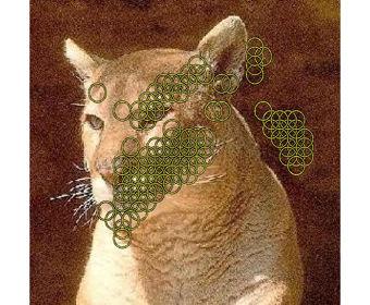
21 Figure 3.3: An example of a heterogeneous cluster due to inconsistent matching between image features. The thickness of the lines indicate the strength of the match, i.e. thicker lines indicate higher matches. The Okapi image has been grouped with the four Face images due to its high pair-wise matching similarity with each Face image. However, an okapi feature that matches highly with one face image does not necessarily match highly with another face image the high matching features across images are inconsistent. Although not shown here, the Face images would have high matching features that are consistently on the face regions (the foreground). across all intra-cluster pairs). The flow field specifies which features in two images best match which, and using what amount of weight. Given a cluster containing C images {X 1,...,X C }, for each example X i, i = 1,...,C, we define (C 1) X i - dimensional weight vectors denoted w ij, with j = {{1,..., C} \ i}. That is, we compute a vector of feature weights for the i-th example against every other image within the cluster. Each of the weight entries in w ij specifies how much 15

22 its feature from X i contributed to the match with set X j. We define the d-th element as w ij (d) = X j p=1 F ( d,p D f (X i ) d,f (X j ) p ), for d = 1,..., X i. Each weight is the sum of all the flow amounts from that particular feature in X i to any other feature in the other set X j, normalized by the inter-feature distance between the matches (we use L 2 ). We compute the final weights {w 1,...,w Xi } as the element-wise median of these (C 1) vectors, normalized to maintain the original total weight. The final weights give a robust estimate of how much each feature consistently matched with other features in intra-cluster images. High weighted features in an image will indicate that they have good consistent matches throughout the intra-cluster images, while low weighted features will indicate that they have inconsistent matches throughout the intra-cluster images there may be a few good matches, but the matches are not consistent enough to produce high weights. Specifically, for a feature to obtain a high weight, it must have high matches to features belonging to at least half of the intra-cluster images. We normalize the final weights to maintain constant total weight per image, such that X i p=1 w p = X i. This prevents weights attached to an irrelevant example from wasting away to nothing and getting stuck in their initial cluster. For example, if a Face image has been incorrectly assigned to a cluster comprised mostly of Okapis, its final features might all have very low weights. By normalizing the final weights to maintain constant total weight, the features in the Face image have a chance to match with other Face images features in the ensuing iteration. In general, if a clump of images in a cluster contains instances of the 16

23 same category, high weights will be attributed to their consistently re-occurring parts the foreground. Note that depending on the current cluster membership, the updated feature weights can be quite different from the weights that were used to compute the clusters. To begin the next iteration, we re-compute the flows and affinities between all pairs of all N examples using the new weights, and re-cluster. As the weight distributions shift, subsequent leastcost matches are biased towards matching those features more likely to be foreground. We iterate between the matching, clustering, and re-weighting, until there is no change in the cluster assignments or until the average percent change in weight is below a threshold. In practice, we observe the most impact from the first several iterations (see Chapter 4). Essentially, our method updates the weights on the features of each image to produce tighter clusters in the next iteration. This is possible because our feature updates guarantee that the matching cost between two images decreases when compared to the matching cost obtained prior to the weight updates. Our algorithm then chooses the weights (by the median) for each image such that the overall matching cost between the intra-cluster images decreases. Therefore, subsequent iterations produce tighter clusters. Due to the complexity of computing the optimal matching on weighted point sets, which is greater than O(n 3 ) where n is the number of features, in practice we compute the matrix C with a variant of the pyramid match kernel (PMK) algorithm [15]. The PMK approximates the least cost match for unweighted sets in linear time in the number of points in a set by inter- 17

24 secting multi-resolution histograms computed in the feature space (see [15]). Though defined for unweighted point sets, we can apply weights by scaling every histogram bin increment by the weight attached to that point. Given two multi-resolution histograms computed from two feature sets, for every intersecting bin, we compute the optimal matching between the features from both sets that share the bin. We record the flow and cost that each point at the current resolution level contributes to the match; any remaining weight is propagated to the next coarser pyramid level and can be used in future matchings. Zero-weighted features at any level do not contribute to the match. In the end, when all bins have been intersected, we have accumulated the approximate flow and match cost. Each per-bin flow computation is super-linear in the intersection value, but feature space partitions given by the pyramid result in small and gradually increasing intersection counts. While the authors of [16] suggest using weights to affect PMK matching cost, they do not compute flow fields that are influenced by the weights. More importantly, their clustering method is a one-shot process that does not benefit from the mutual updating between clusters and feature weights. Instead, they rank the images according to intra-cluster similarity to identify the prototypical examples for each object category (cluster), which are then used to learn a classifier to label novel instances. 18

25 3.2 Semi-Local Proximity Distribution Descriptors Our algorithm description thus far implies an orderless set-of-features representation. We propose a novel semi-local region descriptor that encodes the appearance and relative locations of other features in a spatial neighborhood. Our descriptor is inspired by the proximity distribution kernel [22], which compares images described by cumulative histograms of nearby visual word pairs. However, while their approach summarizes an entire image with one histogram, we design a proximity distribution feature for each interest point, which makes it possible to use rich local configuration cues within an explicit, weighted matching (and thus calculate the flow as described above). As mentioned in Chapter 2, previous methods that encoded the semi-local neighborhood information failed to either capture the spatial configuration, spatial ordering, or spatial count of the features in the semi-local neighborhood. Our descriptor is built with the motivation to capture all of the above information, and we show in our experiments that it can lead to better object localization and classification performance. We extract local patch features at all interest points. Then we construct a standard n-word visual vocabulary by clustering a random pool of descriptors (we use SIFT [25]) extracted from the unlabeled image dataset, U, and record each feature s word type. We use the k-means algorithm for clustering. For each patch in an image, for each of four directions (quadrants) relative to its center, we compute a cumulative distribution that counts the number of each type of visual word that occurs within that feature s r spatially nearest 19

26 Figure 3.4: Schematic of the proposed semi-local descriptor. The base feature is p. The ellipses denote the features, their patterns indicate their corresponding visual word types, the numbers indicate their rank order of spatial proximity to the base feature, and the q i s denote the four quadrants (directions) relative to p. Here the nearest neighboring feature to p is the feature in q 1 corresponding to the vertically textured word type, and so its bin in H 1 is incremented. For H 2, the bins corresponding to the word types of the two nearest neighboring features to p are incremented the vertically textured word type feature in q 1 and the clear word type feature in q 4. The process is repeated until all R spatially nearest features to p are observed. In this example, R = 6. (Best viewed in color.) neighbor features, incremented over increasing values of r (see Figure 3.4). More precisely, consider an image with patches {p 1,...,p m } and their associated word types {v 1,...,v m }. For each p i, we construct R total 4ndimensional histogram vectors H r (p i ), for r = 1,..., R. In each, the first n bins represent quadrant 1, the next n bins represent quadrant 2, and so on. Each n-length chunk is a histogram counting the number of occurrences of each word type v j within p i s r spatially nearest feature points, divided into 20

27 quadrants relative to p i. Note that higher values of r produce a vector H r (p i ) covering a spatially larger region. Finally, our semi-local descriptor for p i is the concatenation of these R histograms: f(p i ) = [H 1 (p i ),...,H R (p i )]. Every patch s R 4n-length vector is a translation-invariant encoding of neighborhood appearance and coarse geometry. (We can add rotation invariance by setting quadrants based on a feature s dominant gradient; we have not yet explored this variant.) Due to the high-dimensionality and correlation among dimensions, we compute compact descriptors using Principal Components Analysis (PCA). Matching sets of our descriptors does not explicitly enforce spatially contiguous regions to be discovered. However, due to their spatial extent and overlap, individual point matches are in fact dependent. Recent work on sampling strategies shows that the single most important criterion for recognition performance tends to be the number of patches detected in each image [28]. Hence, dense sampling is shown to often yield better recognition accuracy than interest-point detectors, because it provides more coverage of the image. The region that our semi-local descriptor encapsulates can be quite different depending on the sampling method for the base features. Dense sampling on uniform grid points will produce semi-local regions that are consistent in area (in terms of image coordinates) for each feature (except those that lie near edges or corners) independent of the image it belongs to, which could assist in better matching if the objects occupy similar sized regions across images. However, if the foreground objects in different images do not have 21

28 the same scale, the foreground coverage of the semi-local descriptor in each image will be different even if the base feature covers the same part of the object in the images. To make the descriptor scale invariant for densely sampled features, multi-scale sampling can be used where the sampling points are adjusted with respect to the size of the patches, i.e., finer sampling for smaller sized patches. Matching can then proceed between cross-scale descriptors. Sparse sampling with interest point detectors will produce scale invariant semi-local descriptors that are independent of the spatial area in terms of image coordinates. An exception can occur for images containing objects at very different resolutions, since different sparse points will be detected (i.e., a high resolution view of an object may result in more detections with interest point detectors than a low resolution view of the same object). In this case, scale invariance can be approximated by using scale-invariant feature detectors and considering only similarly sized features in the base feature s neighborhood. This way, the semi-local neighborhoods in different images would capture similarly sized regions with respect to the scale of the objects, independent of the image resolution. The tradeoff with dense sampling is that sparse sampling produces less coverage of the image, and not all parts of the foreground object may be captured by the descriptor. Related methods for encoding the appearance of semi-local neighborhoods have been previously proposed. Quack et al. [30] employ a neighborhoodbased image description of visual words in which the scale of the neighborhood is determined by the size of the region of interest (detected feature). Multiple 22

29 instances of the same visual word are not counted, and the neighborhood descriptions are not used explicitly for matching. Instead, the object category is determined by the set of words in a region using data mining tools. Similarly, Sivic and Zisserman [37] represent the neighborhood of each region of interest by encoding the set of the R spatially nearest words to a base feature as a n-d vector, where n is the size the of vocabulary. Agarwal and Triggs [2] construct hyperfeatures descriptors collected hierarchically in increasing neighborhoods of the image space. The difference between these methods and our descriptor is that our descriptor considers the order of spatial proximity as well as the spatial direction in which the neighboring features are located with respect to the patch center. This is a richer description of the semi-local neighborhood of a feature; in order for two descriptors to have a high match, having similar features in their semi-local neighborhoods is not enough the neighboring features must also have similar geometric configurations. Lazebnik et al. [19] proposed to represent an image as a spatial pyramid. An image is repeatedly subdivided and histograms of features are computed over the sub-regions, thereby capturing both the appearance information as well as the spatial layout information of the features. However, their representation is global the partitioning of the regions is based on the image coordinates, and the image as a whole is represented. In contrast, our semilocal descriptor captures information specific to each feature s neighborhood. This suggests that the local representation would fare better in terms of object localization and be more robust to clutter and occlusion for image classification 23

30 tasks. 3.3 Discussion What are the assumptions of our approach? For a pattern to be discovered, it must have support among multiple examples in the collection. Further, only visual patterns that share some configuration of similar semi-local regions can ever be found (e.g., using standard gradient-based region descriptors, our method will not discover a single cluster consisting of both soccer balls and volleyballs, but it can discover a group comprised of different people s faces). Finally, some support for a pattern must be detected in the initial iteration for progress towards refining that pattern to be made in the remaining iterations. Note that features that are strictly speaking background can also earn high weights, if they happen to consistently re-occur with the same foreground class. So, what is learned depends on what the collection U contains: for example, if bikes are typically against a bike rack, then we can expect the pattern to be found as a single entity. The same holds for images with multiple objects that repeatedly co-occur for example, if computer monitors always exist on desks. This is a natural outcome for unsupervised learning from static images (e.g., nothing can indicate that the bike and rack are not one composite object unless they often occur separately), and satisfies the problem definition. This also means that the discovered patterns will not always correspond to the foreground objects, i.e., the dataset will not necessarily be partitioned in concurrence with object class labels. This is because the feature weight 24

31 updates depend strictly on the intra-cluster matches. For two objects that typically occur in the same setting, e.g., cows and sheep, our method may find the co-occurring visual pattern to be part of the background, e.g., grass. The dataset will be partitioned accordingly, in which case we may not end up with a cow-cluster and/or sheep-cluster. This is still a perfectly reasonable outcome, since our method will have found the most consistently co-occurring visual patterns. Semi-supervision can be added to guide the algorithm to learn objects under a certain criterion. For the cows and sheep example, we could take a few images from each category, and remove all features on the grass (the background) by setting their weights to 0. This way, our algorithm would be biased towards finding the re-occurring patterns that fall on the foreground. We could also enforce high (low) affinity in the kernel matrix between some examples that are constrained to be similar (dissimilar). This would be especially helpful for examples with a lot of background clutter that are often misclassified. 25

32 Chapter 4 Results In this chapter we present experiments both to analyze the mutual reinforcement of foreground and clusters, and to compare against existing unsupervised methods. We work with images from the Caltech-101 [3] and Microsoft Research Cambridge v1 (MSRC-v1) [39] datasets, both because they provide object segmentations that we need as ground truth to evaluate our foreground detection, and because previous related unsupervised techniques were tested with this data. Unless otherwise specified below, we sample SIFT features at regular image intervals. 4.1 Implementation Details To determine when to stop iterating, we measure the percent change in the average feature weight change in all images from one iteration to the next, and stop once it slows to 15% or less (a threshold we set arbitrarily). When clustering, we set k as the number of classes present in the dataset in order to evaluate how well the true objects are discovered. Note that k can be set higher to allow sub-categories, e.g., rear-view, side-view of the car category, to be discovered. The number of clusters can be automatically determined by the 26

33 self-tuning spectral clustering method [41], which was demonstrated in [20] to find different aspects/views of tourist attractions. However, on the datasets that we work with, the self-tuning method does not produce enough clusters (usually much less than the number of categories). In practice, we have found that setting the number of k to be equal to the number of categories produces the best clusters (consistent with the images class labels). We fix the neighborhood parameter at R = 64, following [22], which means that each descriptor covers about 1th to 1 th of the image in width and 4 5 height. The vocabulary size n as well as the final dimensionality d (corresponding to the eigenvectors with the d largest eigenvalues after PCA) of the spatial descriptors are varied depending on the number of input images in an attempt to get good coverage. For a dataset that has many object categories (each having distinct appearances and shape), we expect to need a larger vocabulary to capture the variability of the data. On the other hand, too many visual words could also produce very distinct descriptions of neighborhoods in which there are few good matches. The final dimensionality of the descriptor determines how much of the original information of the neighborhood region is retained, so having more dimensions will produce more specific descriptors. However, if the dimensionality is too high, then we will not get good matching with the descriptors due to the curse of dimensionality in very high dimensions, most of the feature space consists of the corners of the hypercube. Therefore, n and d are chosen with the above taken into consideration. The specific numbers will be stated in the appropriate sections below. 27

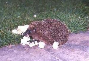
34 To construct the pyramid tree for the modified PMK algorithm, which is used to approximate the EMD, we randomly sample features from the data to represent the feature space, and partition the feature space with hierarchical k-means clustering (with Euclidean distance). The number of levels, L, and branches, B, of the tree are user-defined parameters we typically use 10 branches with four or five levels. 4.2 Analyzing the Effects of Mutual Foreground/Clustering Reinforcement While some classes in the Caltech-101 are fairly clutter-free, we purposely select categories with the highest clutter in order to demonstrate our method s impact. To do this, we first built supervised classifiers on all 101 categories: one trained with all image features, and one trained using only foreground features. Then we ranked the classes for which segmentation most helped the supervised classifier, since these directed us to the classes with the most variable and confusing backgrounds. In this way, we formed a fourclass (Faces, Dalmatians, Hedgehogs, and Okapi) and 10-class (previous four plus Leopards, Car Side, Cougar Face, Guitar, Sunflower, and Wheelchair) set. Figure 4.1 shows example images of the two sets. For each class, we use the first 50 images. We set n and d to 200 and 100, respectively, for the four-class set, and 400 and 130, respectively, for the 10-class set. The numbers are chosen arbitrarily (they are not exhaustively tuned), with the intent that they provide good coverage of the datasets. For this experiment, we discard 28

35 any contrast-free regions. If our algorithm correctly identifies the important features, we expect those features to lie on the foreground objects, since that is what primarily re-occurs in these datasets. To evaluate this, we compare the feature weights computed by our method with the ground truth list of foreground features. We quantify accuracy by the percentage of total feature weight in an image that our method attributes to true foreground (fg) features. To make values comparable across images and classes, we compute fg, where fg and bg denote fg+bg the sums of all foreground (background) weights normalized by the number of all foreground (background) features, respectively. If all weights were on foreground, the score would be 1, while if all weights were on background, the score would be 0. Figure 4.2(a) evaluates our method s unsupervised foreground selection for the two datasets across iterations. All features start with uniform weights, which yields a base score of 0.5. Then each image s weights continually shift to the foreground, with significant gains for most classes as the clusters continue to be refined. In the 10-class set, the Hedgehog class improves more slowly. Upon examination, we found that this was due to many hedgehog images dispersed across the initial clusters, resulting in more gradual convergence and cluster swaps. As our method weights foreground features more highly, we also expect a positive effect on cluster quality. Since we know the true labels of each image, we can use the F-measure to measure cluster homogeneity. The F-measure 29

36 Figure 4.1: Examples of images belonging to the four-class and 10-class sets of the Caltech-101 dataset. The first four rows belong to the four-class set. 30

37 foreground accuracy scores Caltech classes subset Faces Dalmatians Hedgehog Okapi iterations Fmeasure Caltech classes subset Quality with our unsupervised approach Quality with perfect ground truth segmentation iterations foreground accuracy scores Caltech classes subset Faces Leopards Car Side Cougar Face Dalmatians Guitar Hedgehog Okapi Sunflower Wheelchair iterations (a) Quality of foreground detection Fmeasure Caltech classes subset 0.62 Quality with our unsupervised approach Quality with perfect ground truth segmentation iterations (b) Quality of clusters formed Figure 4.2: Evaluation of feature selection and category discovery on the Caltech dataset. (a) The average foreground scores over iterations for all images from the 4-class (top) and 10-class (bottom) sets from the Caltech-101. (b) The cluster quality for those sets. The black dotted lines indicate the best possible quality that could be obtained if the ground truth segmentation were known (see text). 31

38 measures the degree to which each cluster contains only and all objects of a particular class: F = i n i max n j F (i, j), where F (i, j) = 2 R(i,j) P(i,j), and R(i,j)+P(i,j) P and R denote precision and recall, respectively, and i indexes the classes and j indexes the clusters. High values indicate better quality. Figure 4.2(b) shows the impact of foreground detection on cluster quality. To provide an upper bound on what quality level would result if we were to have perfect foreground segmentation, we also evaluate clusters obtained using only the foreground features (black dotted lines). Note that without any supervision or foreground/backgrouind annotation, our approach clusters almost as well as the ideal upper bound. Also, as we iterate, the better foreground weights incrementally improve the clusters, until quality levels out. Figure 4.3 illustrates example results in which our method finds good support on the foreground. Note that we show the central base features to our semi-local descriptors. These examples have the highest foreground scores in each category and are always associated with the correct cluster, e.g., the guitar image belonging to a cluster almost entirely comprised of guitars. Figure 4.4 illustrates example results where our method weights foreground features highly, but also mistakenly finds good support for some background. Again, we show the base features to our semi-local descriptors. These examples have the lowest foreground scores in each category and are almost always associated with the incorrect cluster, e.g., the guitar image belonging to a cluster almost entirely comprised of leopards. These results confirm what is expected, since the majority-class images in a cluster will have the highest 32

39 Figure 4.3: Examples showing the highest weighted features per image. In these examples, our method attributes weight almost only to foreground features. Note that we show the base features to our semi-local descriptors. Figure 4.4: Examples our method does most poorly on: it weights foreground features highly, but also (mistakenly) finds good support for some background. Note that we show the base features to our semi-local descriptors. 33

40 weighted features on the foreground, while the outlier images will have the highest weighted features on regions other than (or possibly in addition to) the foreground. Note that our algorithm finds meaningful features by definition, reoccurring visual patterns in the cluster images. Therefore, this does not imply that all foreground features are meaningful. Only those that re-occur across images in a cluster are meaningful. Furthermore, even some background features may be meaningful, e.g., features that capture parts of the street in car images, since cars are commonly found on the street. (If this were a supervised feature selection task, it may even be favorable to include background features if we knew that those features were part of regions that were visually re-occurring patterns across the foreground images.) Our assumption for this experiment is that the backgrounds are uncorrelated, and therefore the foreground features are the only meaningful features. This property usually does not hold in real images, but we can still expect to get better clusters with our method as long as the re-occurring patterns are weighted highly. Figure 4.5 shows an example of the refinement of clusters and weights over iterations on the four-class set. The highest weighted features are shown in yellow, and are features that have weight greater than 1.75 a high value given the distribution of weights in the data. The first row of clusters shown for each iteration are those that are comprised mainly of the Dalmatian images. We focus our illustration on the Dalmatian cluster images. In the first iteration, after pairwise image matching and clustering has been performed, 34

41 Iteration 1 Iteration 2 Iteration 3 [ ] [ ] [ ] [ ] [ ] [ ] [ ] [ ] [ ] [ ] [ ] [ ] Figure 4.5: Example cluster and weight refinement on the 4-class set. The highest weighted features are shown in yellow. The actual number of images in a cluster for [faces, dalmatians, hedgehog, okapi] is shown below. Images displayed are sampled proportionally to the actual number of images per class in each cluster. Note that as the cluster quality improves, our method weights features on the foreground more highly. 35

42 about 60% of the cluster images belong to the Dalmatian class, as a result of their common foreground support leading to good matches. The rest belong to the Okapi and Hedgehog classes, due in part to some of their features (both from foreground and background) having good support with other intra-cluster images (including Dalmatian images). Note that high matches for these outlier images are still possible, but it is likely that each matching draws from different combinations of features. Similar results are found in each of the other three clusters, comprised mainly of Face, Okapi, and Hedgehog images, respectively. The ensuing feature weight updates lead to the highly weighted foreground features for the Dalmatian images. The outlier images will have weights distributed fairly evenly across foreground and background features the highly matching features for an outlier image are inconsistent over pairwise matches to intra-cluster matches. While some outlier images may still have consistent foreground support among each other, e.g., the three Okapi images, the final updated weights will not reflect those agreements since the median values are taken among all intra-cluster matching features weights. The combination of highly weighted foreground features on the Dalmatian images, and (approximately) evenly distributed weights on the outlier images produces a better quality cluster in the following iteration; at iteration 2, about 70% of the cluster are comprised of Dalmatian images. Finally, at iteration 3, 77% of the cluster images belong to the Dalmatian class. In general, it is hard to expect perfect clusters to be formed based on class labels. The 36

43 semi-local features capturing the appearance in semi-local neighborhoods of an Okapi image could happen to appear more similar to that of a Dalmatian image than to that of other Okapi images. However, in most cases, consistent visual patterns can be expected from images belonging to the same class, and thus, with good foreground support in the first iteration, improvements in cluster quality will result over iterations. We also evaluate our method s unsupervised foreground discovery and category learning on the MSRC-v1 dataset. The dataset is comprised of 240 images belonging to 9 object classes, and has more clutter and variability in the objects appearances than the Caltech-101 dataset. The object categories are Horse, Sheep, Tree, Building, Airplane, Cow, Face, Car, Bicycle. The dataset creators state that there are not enough training regions to learn reasonable models of horses and sheep we remove the first 30 images of the dataset which correspond largely to these classes. Therefore, our revised dataset consists of seven classes with 30 images each. Examples of images in this dataset are shown in Figure 4.6. For this experiment, we set n to 400 and d to 130. Figure 4.7(a) evaluates our method s unsupervised foreground selection for the dataset across iterations. Again, improvements in foreground discovery over iterations is evident. Categories which have slower improvement, e.g., Tree, are those that are more likely to be confused with background, e.g., grass. We also evaluate overall cluster quality using the F-measure, which is shown in Figure 4.7(b). The black dotted lines indicate the upper bound on the quality level which is found by evaluating clusters obtained using only 37

44 Figure 4.6: Examples of images belonging to the MSRC-v1 dataset. 38

45 foreground accuracy scores Tree Building Airplane Cow Face Car Bicycle MSRC dataset iterations Fmeasure MSRC dataset 0.64 Quality with our unsupervised approach Quality with perfect ground truth segmentation iterations (a) Quality of foreground detection (b) Quality of clusters formed Figure 4.7: Evaluation of feature selection and category discovery on the MSRC dataset. (a) The average foreground scores over iterations for all images from the seven classes of the MSRC dataset. (b) The cluster quality for those sets. The black dotted lines indicate the best possible quality that could be obtained if the ground truth segmentation were known (see text). foreground features. As our method weights foreground features more highly, we see improvement in cluster quality. However, the increase is not as significant compared to that seen on the Caltech-101 dataset. This is because the MSRC-v1 has a lot of correlated background many objects are situated on grass and therefore the meaningful features found are often on the background. This resulted in some of the initial clusters being grouped based on the background features and improvement on those clusters (in terms of class labels) could not be made over iterations. (If we were to label the images in which the background features were given the highest weight with grass or sky (instead of cow, airplane, etc.), then we would see an improvement in cluster quality since the background is the most consistently re-occurring visual pattern in those images.) In [6], the authors suggest an approach that 39

46 is robust to perceptual aliasing by modeling the correlation of features in the dataset images. Similarly, standard term frequency-inverse document frequency, tf-idf, down-weights features that are very common across images in the database [36]. These methods could be used to remove the background features if most of the images have similar backgrounds (even among different object categories). However, without prior knowledge of the distribution of foreground and background features in the images, we cannot prevent their method from removing foreground features (along with background features) if they are the most commonly re-occurring features in the images. To overcome the problem of correlated image backgrounds, we could add semi-supervision by removing the background features on some images to bias our algorithm to capture the foregrounds, or adjusting the kernel matrix based on some paired constraints to enforce grouping or separation of some images. We would like to explore these areas in future work. 4.3 Comparison with Existing Unsupervised Methods Next we empirically compare our approach against published results from alternative unsupervised visual learning methods [9,16,23,24]. The authors of [9] propose a clustering algorithm called affinity propagation, where messages between data points are exchanged to find a good partition. The method considers all data points as candidate exemplars and iteratively finds the best set of exemplars that partitions the data. They chose two subsets of the Caltech-101: a 20-class subset composed of: Faces, 40

47 [9] FF-Dense FF-Sparse FF-SIFT Purity (7-class) (%) Purity (20-class) (%) Table 4.1: Comparison with affinity propagation [9] for the seven-class and 20- class subsets of the Caltech 101 dataset in terms of the purity cluster quality measure. We test our method (abbreviated here as FF for Foreground Focus) with three different features: 1) FF-Dense, in which our semi-local descriptor uses densely sampled SIFT descriptors as base features, 2) FF-Sparse, in which our semi-local descriptor uses the SIFT descriptors detected with DoG as base features (the same features as in [9]), and 3) FF-SIFT, in which the DoG SIFT features are used without our semi-local descriptor. Overall, our method performs much better than affinity propagation. Leopards, Motorbikes, Binocular, Brain, Camera, Car Side, Dollar Bill, Ferry, Garfield, Hedgehog, Pagoda, Rhino, Snoopy, Stapler, Stop Sign, Water Lilly, Windsor Chair, Wrench, Yin Yang, and a seven-class subset composed of: Faces, Motorbikes, Dollar Bill, Garfield, Snoopy, Stop Sign, Windsor Chair. Examples of images belonging to the two subsets are shown in Figure 4.8. The first 100 images are taken from each class, and n and d are set to 200 and 100, respectively, for both subsets. In Table 4.1 we compare our method with the same data, using the purity cluster quality measure used in [9]. Purity measures the extent to which a cluster contains images of a single dominant class, Purity = n j j max n i P(i, j), where i indexes the classes and j indexes the clusters, and again P is precision. We first produce results using our algorithm with two base feature types for our semi-local descriptor: 1) densely sampled SIFT descrip- 41

48 Figure 4.8: Examples of images belonging to the seven-class and 20-class subsets of the Caltech-101 dataset defined in [9]. The first seven rows (on the left) belong to the seven-class subset. 42

49 tors, and 2) SIFT descriptors detected using Lowe s Difference of Gaussians (DoG) scale space selection (the same setting as in [9]). A strength of the affinity propagation method is that non-metric affinities are allowed, and so the authors compare images with SIFT features and a voting-based match, which is insensitive to clutter [25]. Still, the clusters found by our method are significantly more accurate, indicating the strength of both our refinement process and semi-local descriptor. Our method using dense base features performs much better than when using sparse (DoG) base features. Since most of the objects in the seven-class and 20-class subsets are of similar size, dense sampling produces consistently sized regions described by our semi-local descriptor throughout the images. More importantly, dense sampling provides better coverage of the objects (foreground) than sparse sampling. We also measure purity for the two subsets using only the DoG SIFT features (without the semi-local descriptor). This is to observe the gain that our semi-local descriptor provides over the local base descriptors. Results are shown in Table 4.1, fourth column. The clusters found using only the DoG SIFT features still produce higher accuracy than that obtained by [9], but lower accuracy than when the semi-local descriptors are built on top of the base features. On the seven-class set, the visual patterns captured in the first iteration corresponded mostly to the foreground objects such that the clusters were of high quality. This improved the foreground detection and cluster quality over iterations. However, on the 20-class set, the cluster quality after the first iteration was not as good the visual patterns found did not entirely cor- 43

50 [16] FF-Dense FF-Sparse Purity (%) ± ± ± 1.10 Prediction Accuracy (%) ± ± ± 1.07 Table 4.2: Comparison with [16] for unsupervised category learning and recognition performance on novel images for the Caltech-4 dataset. Unsupervised category learning is measured in terms of overall cluster purity, and recognition on unseen images is measured in terms of the mean diagonal of the confusion matrix. Results are mean values with standard deviations, averaged over 10 runs with randomly selected training/testing pools. We test our method (abbreviated here as FF for Foreground Focus) with two different features: 1) FF-Dense, in which our semi-local descriptor uses densely sampled SIFT descriptors as base features, and 2) FF-Sparse, in which our semi-local descriptor uses the SIFT descriptors detected with the shape-adapted and maximally stable region detectors as base features. Our method performs better than [16] for both base feature types. Note the robustness of our method shown by the small standard deviations. respond to the foreground. Because the features did not capture any spatial and/or geometrical information, many were erroneously matched, i.e., foreground feature to background feature. This produced weak clusters such that less improvement could be made over iterations. These results show the value of the proposed semi-local descriptor, since they confirm that capturing both appearance as well as semi-local structure improves matching quality. In Table 4.2 we compare against the method of [16], which also forms groups with partial-match spectral clustering, but does not attempt to mutually improve foreground feature weights and clusters as our method does. We use two feature types for base features to our semi-local descriptor: 1) densely sampled 128-dimensional SIFT descriptors (denoted as FF-Dense), and 2) 72-44

51 Figure 4.9: Examples of images belonging to the Caltech-4 dataset. dimensional SIFT features detected with shape-adapted and maximally stable region detectors (denoted as FF-Sparse). Base feature type one will produce many more semi-local descriptors on average per image, than base feature type two. It also allows the semi-local descriptors to cover similarly sized regions across images, which could be useful if the foreground object is consistent in size across images. Base feature type two is more sparse there is less coverage of foreground, but also of background which could potentially eliminate spurious matches yet distinctive. We perform the same unsupervised category learning and classification experiments as prescribed in [16]. In the object category learning experiment, four categories are learned from the Caltech-4 database comprised of 1155 rear views of cars, 800 images of airplanes, 435 images of frontal faces, and 798 images of motorbikes. Example 45

52 images of this dataset are shown in Figure 4.9. We set n and d to 800 and 130, respectively, to account for the large number of images. We achieve better cluster purity with both feature types than [16] (where sparse 10-dimensional Harris-affine SIFT features were used). Results are averaged over 10 runs with randomly selected learning pools of 100 images per class. In the classification experiment, we use the learned categories to predict labels for novel images. We train Support Vector Machines with the PMK using the labels produced by the unsupervised category learning. We classify the remaining images of the dataset (2788 images, ranging from 300 to 1000 per class), where recognition performance is computed as the mean diagonal of the resulting confusion matrix, and average results over 10 runs with the randomly selected pools of training images from the object category learning experiment. Our method gives better prediction for novel examples than [16]. Our algorithm s very small standard deviations in accuracy for both experiments indicate that it is less sensitive to the composition of the unlabeled data, and provides significantly more reliable groupings. This is mainly due to the distinctiveness of our semi-local descriptors, which resulted in more robust feature matches and higher quality clusters. In these experiments, our method performed better using sparse base features rather than dense base features for the semi-local descriptors. Most of the error for either feature type occurred for the airplanes being confused as cars or motorbikes. Upon further examination, we found that the confused images had more background clutter than other Airplane images, and their 46

53 (a) (b) (c) Figure 4.10: (a) an airplane image. (b) With dense sampling, 720 features are detected, of which 119 belong on the foreground object (16.53%). (c) With sparse sampling using interest point detectors, 253 features are detected, of which 125 belong on the foreground object (49.41%). background features were similar to those found on the Motorbike and Car images. We also noticed that the Airplane images on average had the least number of foreground features among the four classes in the dataset, which could have resulted in semi-local descriptions occupied by a lot of background features (see Figure 4.10). Thus, it makes sense that the sparse base features perform better, as the dense sampling detects many more background features. In addition to the semi-local descriptor features, we also evaluate our method using only the 72-dimensional SIFT features detected with shapeadapted and maximally stable region detectors. In Table 4.3, we compare our method using these features as base features to our semi-local descriptor, and our method using only these features (without semi-local information). The interest point detected SIFT features (Sparse) performs much worse than the semi-local descriptors (Semi-Local-Sparse). This again shows the value of our semi-local descriptors that capturing both appearance and geometry in a local neighborhood can produce more informative and descriptive features that are less likely to spuriously match. The initial clusters produced from 47

54 Semi-Local-Sparse Sparse Purity (%) ± ± 3.50 Prediction Accuracy (%) ± ± 3.12 Table 4.3: Comparison between semi-local descriptors and SIFT descriptors for unsupervised category learning and recognition performance on novel images for the Caltech-4 dataset. Unsupervised category learning is measured in terms of overall cluster purity, and recognition on unseen images is measured in terms of the mean diagonal of the confusion matrix. Results are mean values with standard deviations, averaged over 10 runs with randomly selected training/testing pools. We test our method with two different features: 1) Semi-Local-Sparse, in which our semi-local descriptor uses the SIFT descriptors detected with the shape-adapted and maximally stable region detectors as base features, and 2) Sparse, in which the same shape-adapted and maximally stable region detected SIFT features are used without our semi-local descriptor. Our method performs better with semi-local descriptors. the sparse features had low overall cluster purity, and not much improvement could be made over iterations. Finally, Figure 4.11 compares the accuracy of our method s foreground discovery to that of several latent topic models for the Caltech motorbike class, as reported in [24]. Foreground features are determined by ground-truth bounding box segmentations. In [24], two probabilistic Latent Semantic Analysis (plsa) topic models are learned from a combined dataset of the Caltech motorbike class (826 images) and the Caltech background class (900 images). Similarly, we learn two object categories (clusters). The foreground detection rate is computed by varying the threshold among the top 20% most confident features as prescribed in [24]. Interest points are detected using the Hessian- 48

55 Detection Rate Caltech Motorbike Foreground Detection Rate corresp. plsa spatial plsa standard plsa 0.2 FF FF semi local FP per image Figure 4.11: Comparison with several latent topic models for foreground discovery for the Caltech motorbike class. For each method, the foreground detection rate is computed by varying the threshold among the top 20% most confident features in each image. We compare our method with a standard plsa model, plsa with spatial information [23], and a correspondence-based plsa variant [24]. We test our method (abbreviated as FF for Foreground Focus ) with two different features: 1) FF, with Hessian-affine SIFT features (same feature setting as in [24]), without our semi-local descriptor, 2) FF semilocal, in which our semi-local descriptor uses the Hessian-affine SIFT features as base features. affine detector [27], and described by SIFT descriptors. The descriptors are projected down by PCA to 30 dimensions, and n is set to 500. These features and parameters are consistent with those used in [24]. The plsa model was developed in the statistical text literature, and uses the bag-of-words model in which each document is represented as an orderless bag of words. It discovers topics by examining the co-occurring words across documents in the dataset. In the computer vision domain, an image is treated as a document, its features are treated as visual words, and object 49

56 categories are the topics to be discovered. While the idea of discovering categories in an unsupervised fashion is similar to our approach, the plsa model requires that the features in the data be quantized to form a visual vocabulary. Our method does not require this step (although descriptors that require a vocabulary can certainly be used; e.g., our semi-local descriptor). The main difference between the plsa models and our method is that for our method, visual patterns discovered in each image are determined solely by the intra-cluster image matchings. In contrast, for the plsa model, the topics discovered in an image are determined by all the images in the dataset. The impact of this difference is shown below. We compare our method with a standard plsa model, plsa with spatial information [23] that hypothesizes the location and scale of the object, and a correspondence-based plsa variant [24] that considers the configuration of patches belonging to the object. The plsa models compute foreground confidence based on the probability of the topic given the patch. We test our method with two feature types: 1) Hessian-affine SIFT, as described above, and 2) semi-local descriptors with Hessian-affine SIFT as base features. We set d to 130 for both feature types. Our approach outperforms the others for most points on the detection curve, providing much better precision for low false positive rates. Using the semi-local descriptors performs overall slightly better than using the local descriptors, showing that performance gain can be achieved when semi-local appearance and geometric information are aggregated. 50

57 We believe that the plsa models do not perform as well as our method because two topic models are learned for each image on the entire dataset. This means that each image where the true class label is Motorbike will still have a probability (albeit very small) of belonging to the background topic. The probability that a word (feature) belongs to the object, e.g., motorbike, depends both on whether the word occurs repeatedly on the object throughout the dataset, and on the probability of the image belonging to the Motorbike topic model. If an image has a high probability of belonging to the background topic, the words associated with the background topic will have a low probability of belonging to the Motorbike topic possibly incorrectly so. As the confidence of the background topic increases for an image, the probability that foreground features (those on the motorbike) will be incorrectly associated with the background model also increases (and thus their confidences of belonging to foreground decreases). Since many of the Motorbike images have backgrounds that are similar to regions in images belonging to the Background class, the likelihood of this occurring is quite high. While our method may also mistakenly give high weights to background features, the chances are lower as long as the clustering at each iteration partitions the data well. To see why, remember that our method updates the weights after clustering after the dataset is partitioned into two groups, i.e. the Motorbike cluster and the Background cluster. Feature weight updates will then be made dependent only on intra-cluster images, with features belonging to similar visual patterns being weighted higher. Thus, for the Mo- 51

58 torbike images belonging to the Motorbike cluster, the highest weighted features will belong to the foreground. 4.4 Evaluation of our Semi-Local Proximity Distribution Descriptor In previous sections, we have analyzed the classification and foreground discovery of our unsupervised Foreground Focus method on various datasets. In this section, we analyze the performance of our semi-local descriptor by making a direct comparison to the neighborhood-based image descriptor of Quack et al. [30] and to a local alternative, a simple bag-of-words description. The goal of these experiments is to determine how well our semi-local descriptor discovers the same visual patterns (foreground objects) in novel images that occur in the training images. We tie this in with a modified version of our Foreground Focus method for determining the feature weights. The difference with our original method is that, unlike previous experiments, the following are supervised tasks and hence no clustering is involved. We perform the same experiment as in [30], where a bounding box hit rate (BBHR) is measured over the positive test sets. A bounding box hit (BBH) is counted if more than h of the selected features lie on the object (i.e., inside the bounding box) and the BBHR is the total BBH normalized by the total number of object instances in the positive test set. The BBHs are measured by using the ground truth bounding box annotations. The BBHR is measured with respect to the False Positive Rate (FPR) which is the number 52

59 of selected features lying outside of the bounding box divided by the number of selected features, averaged over the entire test set. The selected features are determined by varying the selection threshold over the feature confidences. The idea behind the BBHR is that there should be at least a certain number of features selected for later processes (such as an object recognition system) to operate effectively. Therefore, the metric (i.e., BBHR vs FPR) compares the tradeoff of the number of selected foreground features at the expense of false positives (background features that are mistakenly thought to be on the foreground). The experiment is conducted on three object categories: Bikes, Motorbikes, and Cars Rear. We use the same images from the publicly available datasets and set h to five, as in [30]. We use densely sampled SIFT base features for our semi-local descriptor, and set n to 200 and d to 130. The positive training images use only regions of the image that correspond to the object (inside the bounding box), except for the Motorbikes where full images are used since no ground truth annotation is available. More detail on the datasets corresponding to the object categories are as follows: Bikes. This dataset has 250 positive training, 250 negative training, and 125 testing images of bikes taken from the GRAZ-01 (100 positive training, 100 negative training, and 50 testing) and GRAZ-02 (150 positive training, 150 negative training, and 75 testing) datasets [29], respectively. Motorbikes. This dataset has 826 positive training images taken from the 53

60 Figure 4.12: Examples of positive training and testing images belonging to the Bikes, Motorbikes, and Cars Rear datasets. Caltech-4 Motorbikes database and 200 images randomly taken from the Caltech- 256 [4] background class. There are 115 testing images taken from the TUD Motorbikes [1] dataset. Cars Rear. This dataset has 126 positive training images and 526 testing images of rear-views of cars from the Caltech-4 dataset. The negative training images are 1155 images of street scenes without cars. Examples of positive training and testing images in these datasets are shown in Figure We compare our method with [30], in which a tiled region is centered on 54

61 each interest point to bin nearby visual words. The scale of the neighborhood is determined by the size of the region of interest (detected feature). The confidence of a feature in a test image is measured by counting how often it is part of a neighborhood that matches to mined configurations of the training images. The more matched configurations the feature is part of, the higher its confidence. We also compare our method with the baseline bag-of-words scheme (as defined in [30]), where each visual word is given a weight based on how often it appears in the training images of the given category. Then, each feature in a test image is given a confidence that corresponds to the weight of its matching visual word. In order to make a fair comparison to [30], we modify our unsupervised Foreground Focus method to work with labeled data, and devise a method to set weights on our features discriminatively. Because we are only working with a single dataset at a time, no clustering is involved (and hence no iterations). We compute the weights on our descriptors in the test images as follows. First, each test image is matched to all images in the positive training set. The feature weights for a test image are computed in exactly the same way as in our original Foreground Focus method; we take the median over the weights (which take into account both the mass of the matching features as well as their distances) obtained from the pair-wise matches between the test image and all positive training images. We only select features that have weight greater than one essentially, we are only keeping the features that our method determines to be on the foreground. The remaining feature weights are set to 55

62 zero. Then, the process is repeated, but with the test images matched to the negative training images. Again, we select features that have weight greater than one, which are those that our method determines to be on the background (since this time the test images are matched to the negative training examples). Finally, among the features that our method had determined to be on the foreground, we discard the features that are also determined to be on the background. We are left with a set of features that have high confidence of belonging to the foreground, while at the same time have low confidence of belonging to the background. This procedure is analogous to the way the confidences for the features of [30] are determined, where both the positive and negative training examples are used to find the most distinctive and frequent foreground features that are unlikely to be part of the background. Results on the three datasets are shown in Figure The results of [30] are shown as curves with square markings, the baseline bag-of-words scheme results are shown as curves with diamond markings, and our method s results are shown as curves with triangles. Our semi-local descriptor significantly outperforms the baseline bag-ofwords scheme on all datasets, which confirms that adding geometric and spatial layout information to local appearance descriptors results in better foreground discovery. When comparing to [30], our method performs better on the Cars Rear dataset, comparably on the Motorbikes dataset, and worse on the Bikes dataset. We achieve the best results on the Cars Rear dataset, because the 56

63 Mean False Positive Rate Mean False Positive Rate Bikes [h=5] Bounding Box Hit Rate Motorbikes [h=5] Bounding Box Hit Rate Mean False Positive Rate Cars Rear [h=5] Bounding Box Hit Rate Bag of Words [30] our method Figure 4.13: Bounding box hit rates vs. mean false positive rates for Bikes, Motorbikes, and Cars Rear. Lower curves are better. Overall, our method significantly outperforms the baseline bag-of-words scheme and performs comparably to [30]. negative training images specifically match the backgrounds of the positive training images. Hence, any background feature that may (incorrectly) have high weight of belonging to the foreground (when matching to the positive training images) would have high weight of belonging also to the background (when matching to the negative training images) and would be discarded by our modified Foreground Focus method. This method only considers those features that have high weight of belonging to the foreground and low weight of belonging to the background. The negative training images help less on the Motorbikes and Bikes 57

64 datasets, because they are not specifically chosen to be similar in appearance to the backgrounds that appear in the positive training images. These datasets also have severe clutter in many images, and large object scale and appearance variations. Still, our semi-local descriptor performs well, as can be seen by the low mean FPR even as the BBHR increases. The main difference between our method and [30] is that we do not explicitly train our descriptors to find the most discriminative features. In contrast, the discriminative features in [30] are found by mining the most frequently occurring features in the training images, and then matching the features in the test images to those training images features. Their method is much more selective, as can be seen by the lower maximum BBHR that is obtained on all datasets compared with our method. While a more discriminative approach may reduce false positives, it can also hurt performance for the ensuing object recognition system if there are too few features to work with (even if all of them lie on the foreground). Our semi-local descriptor is able to find many foreground features and still achieve low FPR even at high BBHRs. Hence, our method can be considered to be better than comparable to [30] on the Motorbikes dataset. In terms of the differences in neighborhood-descriptions, we use ranked nearest neighbor (in image space) feature descriptions while [30] uses a tiled grid. The tiled neighborhood description does not count the number of occurrences of the same visual word that falls in a tile it is a set description rather than a bag description. This means that the same descriptions are produced 58

65 for a tile that has many occurrences of the same visual word and a tile that has just a single occurrence of that same visual word. In contrast, our descriptor counts multiple occurrences of the same visual word, regardless of the regions in which they actually fall with respect to the base feature. Therefore, our method can be more specific. The features extracted from street scenes (the negative training images of the Cars Rear dataset) often have very similar appearances. (Let s assume that those features are of the same visual word.) Suppose we have a neighborhood description of a Cars Rear test image, in which the wheel occupies a small region and the rest is occupied by the background (street scene). Our descriptor would have in its neighborhood description, a few foreground features and many background features, while the neighborhood description of [30] might have a similar number of foreground and background features (since the same background word is considered only once in each tile). In this case, our descriptor would be less likely to match with another descriptor that describes only the foreground region (e.g., the wheel and bumper), whereas the tiled region of [30] would have a higher chance of a good match. This could lead to more background features being mistaken as foreground features since the impact of the background features in the neighborhood description is less compared to our descriptor. In terms of orientation, however, our descriptor has a coarser description of where each neighboring feature lies (we only determine the spatial order and in which quadrant the feature lies with respect to the base feature), while 59

66 the tiled neighborhood description of [30] is more rigid since it depends on the actual tile in which a feature falls. Therefore, our descriptor can be more flexible, which can be more robust to deformable objects, e.g., people or animals, or when there are in-plane and/or out-of-plane rotations of the object. Finally, our descriptor encodes all R neighbors of a base feature s neighborhood in its description, while [30] selects the most discriminative features in each tiled neighborhood. While our descriptor can be considered to be more specific (since all nearest neighboring features in a base feature s neighborhood are considered), it can also lead to more clutter features being part of the description (for base features that fall near the edge of the object). This can potentially hurt our descriptor and may have been the reason for its worse performance than [30] on the Bikes dataset. In this dataset, there are many bike images that occupy small and narrow regions of the image. A lot of background clutter may have been considered for each base feature in these regions, which could have led to incorrect high matches between descriptors of the foreground and background regions, and incorrect low matches between descriptors of the foreground and foreground regions. When the objects do not occupy a small region of the image, however, there are many more base features that do not fall on the edges of the objects. In these situations, our descriptors can be very discriminative (and almost clutter free) and can lead to very precise foreground matching. This is confirmed by the good performance of our descriptor on the Cars Rear dataset. Figure 4.14 illustrates example results in which our method finds good 60

67 Figure 4.14: Examples showing the highest weighted features per image found by our modified (supervised) Foreground Focus method. In these examples, our method attributes weight almost only to foreground features. Note that shown here are the base features to our semi-local descriptors. Figure 4.15: Examples our modified (supervised) Foreground Focus method does most poorly on: it weights foreground features highly, but also (mistakenly) finds good support for some background. Note that shown here are the base features to our semi-local descriptors. 61