UNIVERSITY OF CALGARY. Distributed Gaussian Mixture Model Summarization Using the MapReduce Framework. Arina Esmaeilpour A THESIS

Transcription

1 UNIVERSITY OF CALGARY Distributed Gaussian Mixture Model Summarization Using the MapReduce Framework by Arina Esmaeilpour A THESIS SUBMITTED TO THE FACULTY OF GRADUATE STUDIES IN PARTIAL FULFILLMENT OF THE REQUIREMENTS FOR THE DEGREE OF MASTER OF SCIENCE GRADUATE PROGRAM IN ELECTRICAL AND COMPUTER ENGINEERING CALGARY, ALBERTA JUNE, 2016 Arina Esmaeilpour 2016

2 Abstract With an accelerating rate of data generation, sophisticated techniques are essential to meet scalability requirements. One of the promising avenues for handling large datasets is distributed storage and processing. Hadoop is a well-known framework for distributed storage and processing. Further, data summarization is a useful concept for managing large datasets. Data summarization techniques are intended to produce compact yet representative summaries for the entire dataset. Consolidation of these tools can allow a distributed implementation of data summarization. In this thesis, this goal is achieved by proposing and implementing a distributed Gaussian Mixture Model Summarization using the MapReduce framework (MR-SGMM). The main purpose of the proposed method is to summarize a dataset with a density-based clustering algorithm called DBSCAN algorithm, and then summarize each discovered cluster using the SGMM approach in a distributed manner. Testing the implementation with synthetic and real datasets is used to demonstrate its validity and efficiency. ii

3 Acknowledgements First, I am grateful and indebted to my supervisor, Dr. Behrouz H. Far, for his constant help, support and guidance. Also I would like to thank my thesis examination committee Dr. Bijan Raahemi, Dr. Diwakar Krishnamurthy, and Dr. John Nielsen for their constructive comments on the thesis. I would like to express my sincerest thanks and appreciation to Dr. Bijan Raahemi, for his comments based on his intuition and deep insight. I would like to thank my friends and colleagues, Elnaz, Fatemeh and Waeal at Knowledge Discovery and Data mining Lab (KDD Lab) in University of Ottawa for their hospitality and support. I gratefully acknowledge financial support through Mitacs co-funded by Mr. Can Ardic. I was privileged to work as an intern on CrowdAct with an excellent group of engineers at Instalogic. I would like to express my deepest appreciation and love to my beloved family to whom I owe this achievement. My mother, Shahin, I am so pleased and fortunate of having you in my life and thank you for everything you have done for me. Words cannot express my feelings, nor my thanks. My father, Hamid, I miss you and I wish you could be with us and see these days. I would also like to thank my sister, Romina who have always encouraged me through my studies. Words cannot express my special gratitude to my beloved husband, Khabat, for his help, support, patience and endless love each and every day. iii

4 Table of Contents Abstract ii Acknowledgements iii Table of Contents iv List of Tables vi List of Figures and Illustrations vii List of Symbols, Abbreviations and Nomenclature viii 1 Introduction Motivation and problem statement Contributions Thesis structure Literature Survey Data summarization techniques Sampling Probabilistic sampling Non-probabilistic sampling Histograms Micro-clustering Clustering Partition-based clustering approaches Hierarchical clustering approaches Grid-based clustering approaches Density-based clustering approaches Cluster summarization Clustering approaches implemented in the MapReduce framework Partition-based clustering approaches implemented in the MapReduce framework Hierarchical clustering approaches implemented in the MapReduce framework Density-based clustering approaches implemented in the MapReduce framework Technical Constituents Hadoop DBSCAN clustering algorithm Summarization based on Gaussian Mixture Model (SGMM) Finding core points Feature extraction GMM representation of clusters Distributed Gaussian Mixture Model Summarization using the MapReduce framework Partitioning Local processing Merge iv

5 4.4 Reducing the number of SGMM core points in MR-SGMM Summary Experimental results Datasets MR-SGMM testing Partitioning Local processing Merge Data regeneration Figures of merit Core point reduction Efficiency comparison Summary Conclusion and future work Conclusion Limitations and future work Bibliography A Implemented algorithms in java A.1 Partitioning source code A.2 Local processing source code A.3 Merge source code B Single-node SGMM Algorithm v

6 List of Tables 5.1 Differences of Dunn s indexes for regenerated vs. original data for both the MR- SGMM and single-node SGMM approaches Differences of DB indexes for regenerated vs. original data for both the MR- SGMM and single-node SGMM approaches Differences of Dunn s indexes for regenerated and original data for MR-SGMM with all and reduced SGMM core points Differences of DB indexes for regenerated and original data for MR-SGMM with all and reduced core points vi

7 List of Figures and Illustrations 3.1 Schematic description of MapReduce operation Eps-neighborhood of point p. Point p is a core point. Point q is directly densityreachable from point p Density-reachability. Point q is density-reachable from point p Density-connectivity. Point p and point q are density-connected The three steps of the SGMM approach General phases of MR-SGMM Example partitioning phase in the MapReduce framework Creating a grid for a two-dimensional space Example local processing phase in the MapReduce framework A cluster scattered in two partitions Example mrge phase in the MapReduce framework SGMM core points in MR-SGMM and single-node SGMM Geometric shape of datasets Partitioning results for the (a) SDS1, (b) RDS2 and (c) SDS3 datasets. Points with different colors show membership in different partitions. Points with a black color show border points (the joint area between adjacent partitions) Clustering results for (a) partition 1, (b) partition 3, (c) partition 2 and (d) partition 4 in the SDS1 dataset. The x marks in the figure show SGMM core points for clusters (a) Clusters with common border points. The + marks show border points that are also DBSCAN core points. (b) The final clusters Dataset SDS1: depictions of the original (clustered) dataset, SGMM core points and the regenerated dataset for the single-node SGMM (left column, with 269 core points) and MR-SGMM (right column, with 470 core points) Dataset SDS2: depictions of the original (clustered) dataset, SGMM core points and the regenerated dataset for the single-node SGMM (left column, with 358 core points) and MR-SGMM (right column, with 452 core points) Dataset SDS3: depictions of the original (clustered) dataset, SGMM core points and the regenerated dataset for the single-node SGMM (left column, with 250 core points) and MR-SGMM (right column, with 417 core points) Dataset RDS1: depictions of the original (clustered) dataset, SGMM core points and the regenerated dataset for the single-node SGMM (left column, with 288 core points) and MR-SGMM (right column, with 427 core points) Dataset RDS2: depictions of the original (clustered) dataset, SGMM core points and the regenerated dataset for the single-node SGMM (left column, with 579 core points) and MR-SGMM (right column, with 740 core points) Efficiency comparison between single-node SGMM and MR-SGMM vii

8 List of Symbols, Abbreviations and Nomenclature Symbol AGNES CLIQUE DBSCAN MR-DBSCAN DENCLUE DIANA ESP GMM HDFS OPTICS PRBP SGMM MR-SGMM STING Definition AGglomerative NESting CLustering In QUEst Density Based Spatial Clustering of Applications with Noise MapReduce-based DBSCAN DENsity-based CLUstEring DIvisive ANAlysis Even-Split Partitioning Gaussian Mixture Model Hadoop Distributed File System Ordering Points To Identify the Clustering Structure Partition with Reduced Boundary Points Summarization based on Gaussian Mixture Model MapReduce-based SGMM STatistical INformation Grid viii

9 Chapter 1 Introduction 1.1 Motivation and problem statement Data analysis has become an essential element in decision-making for small businesses, large corporations and government. The ever-growing rate of data generation provides an opportunity to explore emerging patterns and uncover non-trivial correlations among many and diverse sources of data. These data sources include client information of financial institutions, commercial enterprises and hospitals. Real-time systems, such as sensor networks and monitoring systems, constantly produce potentially valuable data. Data from weather stations, censuses and geographic information systems can be analyzed to explore new information relationships that have never been accessible before. Individual people constitute billions of sources of data generation by using services, mobile applications, social networks, etc. Means are needed to store, process, analyze and mine all of these massive sources of data [1]. The desire to exploit stored data to extract useful and previously unknown information has led to the development of data mining techniques to analyze large amounts of data. However, the rates of data production and collection have been growing much faster than our ability to process these sources of information. Therefore, it is essential to develop better processing algorithms that rely on distributed storage and computing systems [1]. Improving hardware performance by constructing larger servers and storage arrays may appear to be a solution for handling voluminous data. This approach is generally referred to as scale-up. An important disadvantage of scale-up, however, is that processing time will ultimately be limited by the time required for data transfer among different parts of the server (e.g. between storage and processor). In addition, this seemingly simple solution can become prohibitively expensive for 1

10 data processing beyond a certain scale [2]. An alternative approach to scale-up is scale-out, wherein multiple servers perform the data processing. Additional servers can be added to accommodate increasing needs for storage and processing of larger volumes of input data. The cost of data processing in such a structure will increase linearly with respect to input data size. In comparison with scale-up, scale-out is more cost-effective and flexible for managing growing data sources [2]. Distributing data processing tasks in a scale-out architecture requires careful data partitioning, reassembly and task scheduling across clustered machines, as well as logic to handle individual node failure. Apache Hadoop is an open source framework for managing scale-out architecture [2]. Hadoop operates on a network of commodity machines in one location, and is composed of a Hadoop Distributed File System (HDFS) for storage, and MapReduce for processing. HDFS and MapReduce work well together, with map and reduce functions performed on data stored in HDFS nodes [2]. Another way to help deal with massive data is data summarization. Summarized data is easier to handle, as it requires less storage space, and consequently takes less processing time to analyze. Data summarization techniques allow use of a compact and viable representation of a dataset [3]. It is desirable to summarize data where original data is disposed and only key information is stored on the hard drive for secondary applications. For example, one can use the summarized clustering results for classification of new incoming data without recalling all data points. In addition, simple tasks such as averaging can be performed on the summarized data without relying on recalling all data points. Clustering is a data mining technique that can be used to summarize data. After clustering, data in the produced clusters can be summarized to reduce the required storage and processing time, as preserving all cluster members is typically not feasible for large volumes of data. Several cluster summarization techniques have been developed to meet requirements for different applications and types of data [4, 5, 6]. 2

11 1.2 Contributions As noted, the accelerating growth of data leads to an ever-increasing demand on data processing systems. Even though data summarization is effective in reducing storage requirements for large data sources, implementing data summarization techniques on large data sources can be prohibitively computationally demanding. Therefore, developing data summarization techniques within scale-out frameworks can be an important step toward a sustainable solution for growing data processing requirements. Such a development can benefit from cost-effective, flexible and scalable processing capabilities within scale-out architecture for clustering and summarizing large data sources. In this thesis, this goal is met by implementing a density-based clustering and a cluster summarization technique using the MapReduce framework. Specifically, the work is focused on a MapReduce-based implementation of clustering with a Density-Based Spatial Clustering of Applications with Noise (DBSCAN) algorithm [7], and Summarization based on Gaussian Mixture Model (SGMM) [6]. Both of these techniques are advantageous in discovering and summarizing arbitrary-shape clusters [6, 7]. DBSCAN is a density-based clustering algorithm, which finds clusters based on the concept of connecting dense regions, and discovers arbitrary-shape clusters [7]. The cluster summarization step is done via SGMM, which finds dense regions in a cluster, represents each dense region with a point called an SGMM core point, and delineates features related to the core point. Finally, the SGMM method is used to create a Gaussian Mixture Model (GMM), which is a combination of a set of normal distributions over all SGMM core points of the cluster, and can be used for a compact representation of the original data. The distributed data clustering and summarization approach in this thesis involves the following elements: data partitioning local clustering based in DBSCAN 3

12 cluster merging and data re-assembly data summarization with SGMM data regeneration based on GMM These elements are implemented in a MapReduce framework to ensure scalability for handling large datasets. The implementation is tested on synthetic and real datasets, and its output and efficiency is compared to a non-distributed approach for validation. In addition, a core point reduction approach is proposed and implemented for more efficient and yet accurate data summarization and regeneration. Note that MapReduce-based implementation of DBSCAN algorithm has been studied in [8, 9, 10] that are relying on different partitioning strategies. In this thesis, a grid-based partitioning approach is used for an implementation of DBSCAN algorithm that is compatible with GMM summarization, which are both completely developed in the MapReduce framework. 1.3 Thesis structure The thesis is organized as follows. In chapter 2, a literature survey is presented on data summarization techniques, including clustering approaches and methods of cluster summarization. Clustering approaches implemented using the MapReduce framework are also reviewed. In chapter 3, the technical methods underpinning this thesis are described. This includes the Hadoop framework, DBSCAN clustering algorithm and SGMM algorithm for cluster summarization. In chapter 4, the general structure of the proposed new MapReduce-based SGMM (MR-SGMM) and its constitutive steps are explained in detail. Experimental methods and results to assess MR-SGMM are described in chapter 5. Chapter 6 includes a conclusion and discussion of possible future work. 4

13 Chapter 2 Literature Survey Nowadays massive amounts of data are being generated by activities such as web surfing, using social networks and services, shopping and online bank services. In addition to increase in amounts of generated data, also the rate of increase is drastically high. The management and use of the accumulated large volume of data requires not only large storage devices but also substantial processing, analysis and retrieval methods. A way to mitigate these problems is to summarize the data, reducing storage, processing and retrieval needs. Data summarization techniques are intended to produce summaries which are compact yet representative of the entire dataset. Clustering can be used as a summarization technique. For large volumes of data, preservation of all cluster members is not feasible, so each produced cluster can be summarized as well. Cluster summarization aims to represent a cluster with fewer instances, while preserving the original shape and distribution of the cluster. Summarization approaches are costly, requiring substantial processing time and memory to create a summary for large amounts of data. In this case, distributing data and computation across a cluster of machines can be beneficial. The MapReduce framework provides a means to implement a model for automatically distributing and parallelizing processes in a cluster of commodity machines. In this chapter, section 2.1 gives a survey of the literature on specific data summarization techniques, including sampling, histograms, micro-clustering and clustering. These summarization techniques can be applied to large quantities of data [3]. In section 2.2, cluster summarization methods are reviewed. Finally, clustering approaches implemented using the MapReduce framework are presented in section

14 2.1 Data summarization techniques Data summarization aims to compactly represent large-volume data. The resulting size reduction simplifies the requirements for data storage, retrieval and analysis. Reducing the size of data must facilitate approximate yet informative results in data analysis, complying with requirements in terms of time, space and cost [3]. With the increasing rate of global data generation, data summarization can be applicable to a variety of data sources in different fields and applications. For example, research in astronomy, the earth sciences and medical informatics rely on large sources of data. Data summarization techniques could be employed to categorize data or extract crucial medical information in a more time-efficient manner. Social networks and the World Wide Web are other examples of big data sources. Summarization could play an important role in network and web analysis. Further, mining large amounts of data for analysis of purchasing patterns, stock trends or client reviews could be an indispensable aid for business and marketing. Another potential application of data summarization is query processing in sensor networks [3]. Various data summarization techniques have been implemented to address these applications. Some of the well-known techniques are reviewed in the following subsections, including sampling, histograms and micro-clustering. The final technique presented is a clustering approach for data summarization, covering the groundwork pertinent to the remainder of the thesis Sampling Sampling can be defined as the process of selecting a representative part of a population for the purpose of determining parameters or characteristics of the whole population. Therefore, sampling, as a summarization method, can reduce data size and processing time by considering only a portion of a dataset (samples), but which is still informative. This approach can be useful in a variety of applications, such as data management, approximate query answering, statistic estimation and data stream processing. 6

15 There are two main groups of sampling techniques, probability-based and non-probabilitybased [3]. All techniques are based on a few key elements: Sample: A sample is representative subset of a population that retains the characteristics of the population. Population: A large dataset that can be represented by samples. Frame: A subset of the population that sampling is applied to. Aim of sampling: The main goal of sampling is generalizing a conclusion inferred from studying samples to the population. Sampling error: Sampling error, or statistical error, characterizes the difference between the sample which is observed and the population that is not observed. Sampling bias: Sampling is biased when the probability of selecting individual data points form a dataset is not uniform, resulting in a non-random sampling. There are four common steps in taking a sample of a dataset: 1] define the population (of size N) to be sampled, 2] determine the sample size (n), 3] control for bias and error, and 4] select the sample [3]. In sections and , some well-known sampling methods are described within the two main categories of probabilistic (unbiased) and non-probabilistic (biased) sampling Probabilistic sampling Sampling algorithms having equal probability for all data points to be selected are called probabilistic or unbiased sampling. 1. Simple random sampling is one of the basic sampling techniques, in which all points of the dataset have equal probability for being chosen as a sample in the 7

16 dataset. There are two ways of performing simple random sampling, with replacement and without replacement. In the former, a data point after being selected can be re-selected with the same probability in the next round. In the latter, a data point will be removed from the dataset after being selected, and so cannot be selected again. Random sampling is an easy technique, not requiring substantial information about the dataset in advance. However, access to the population is needed [11]. 2. Systematic sampling uses the sample size n and dataset size N to calculate an interval K = N/n. A random point is selected as a starting point. This starting point is the first sample, K th data point from starting point is the second sample, the K th data point from the second sample is the third sample, and so on. Despite the simple sample selection used in this method, sampling is more accurate than random sampling. However, all data items in the dataset do not have an equal probability of being selected. The probability of being selected depends on the starting point and the interval. Also, patterns in data can be hidden by inappropriate interval selection. Systematic sampling can be a good choice for datasets without any pattern in the data [11]. 3. Stratified sampling divides the population into L non-overlapping areas called strata, with a sample selected from each stratum. If the sample selection method is random sampling, this method will be called stratified random sampling. The sample size for each stratum is calculated in different ways. Optimal allocation is a way to compute sample size proportional to the stratum size, aiming to maximize precision while minimizing cost. Another approach is Neyman allocation, which aims to maximize precision with a given fixed sample size, and computes sample size based on the stratum size and its standard deviation. In this method, dividing the population into proper strata can be difficult, but its accuracy and population coverage are better than those of simple random sampling [11]. 8

17 4. Clustering sampling groups the population into clusters, which should be mutually exclusive and collectively exhaustive. Then, some clusters are selected using random sampling, and the cluster is considered as a sample. Two types of clustering sampling exist, single-stage and multi-stage. In single-stage clustering sampling, all members of selected clusters are considered as a sample. Multi-stage clustering sampling selects data points by random sampling from chosen clusters. The goal of clustering sampling is to reduce cost with respect to an increase in sampling efficiency. Low cost is a particular advantage of this method, but high sampling error is a disadvantage. When clusters are significantly different, cluster sampling is not a good choice because of the high sampling error [3] Non-probabilistic sampling Sampling algorithms for which data points have different probabilities of being selected are considered to be biased or non-probabilistic sampling. Some approaches related to non-probabilistic sampling are accidental sampling [12], quota sampling [13], purposive sampling [11], and snowball sampling [14]. A main disadvantage of non-probabilistic sampling methods is that it may not be easy or even possible to know or prove that a sample is representative of the population. Accidental sampling [12], also known as convenience or opportunity sampling, selects data items from that part of the population that is more available or close to hand. In this method, a chosen sample may not be a good representative for the population. In quota sampling [13], the dataset is divided into mutually exclusive groups, and samples that satisfy a determined proportion are selected from each group. Quota sampling is the nonprobabilistic version of stratified sampling. Quota sampling is appropriate for cases in which processing time is more important than accuracy, the budget is limited or the sampling frame is unknown. 9

18 Purposive sampling [11] chooses samples from a particular population. In [15], purposive sampling is applied in social networks for the purpose of recruitment. In snowball sampling, a data item or a group of data items are first sampled, and they in turn provide further data items to be sampled. Snowball sampling is useful in social network data mining, such as described in [14]. Advantages and disadvantages of sampling Sampling methods are fast and cheap. However, proper sample selection to reduce sampling error can be difficult. There can be bias in the sampling. Selected samples may not adequately represent the population. As a result of sampling, patterns in the population may be obscured in the sample Histograms A histogram is a graphical representation of a data distribution, shown as a set of (attribute value, frequency) pairs. A histogram can be considered to be a data reduction or summarization method, since it represents a large volume of data in a compact way. For nominal attributes, a vertical bar is shown for each value of data, with the height of the bar indicating the frequency of data points with that value. If the attribute is numerical, the data can be divided into disjoint ranges (buckets), with frequencies of data in each of the ranges represented [3]. Some of the more widely used histogram types are described below. Equi-sum or equal-width histograms divide the range between the maximum and minimum attribute values into N intervals (buckets), with equal width. The width of the intervals is equal to (maximum - minimum)/n. Equal-width histograms are not suitable for skewed data [16]. In Equal-depth (frequency) histograms, also known as Equi-height, the range between attribute values is divided into N intervals, such that each interval has approximately equal frequency. Since the computation of interval boundaries can be expensive, this method is not suitable for commercial systems. However, it is a good choice for range queries with low-skew data distribution [16, 17]. A V-optimal histogram categorizes the frequencies of attribute values into a set of buckets in 10

19 such a way that the cumulative weighted variance of the buckets is minimized. In other words, this approach computes the cumulative variance for all possible histograms for a given number of buckets, and selects the histogram with the least cumulative variance among them [18]. The V-Optimal-End-Biased approach [18] groups some of the highest frequencies, some of the lowest frequencies, and the remaining frequencies between them into three individual buckets. V- optimal gives a histogram that represents the original data better and with fewer errors, compared to Equal-width and Equal-depth. However, updating a V-optimal histogram can be more difficult than these other two methods, as sometimes rebuilding of the entire histogram is required. For a MaxDiff histogram, after data sorting a bucket boundary is selected between two adjacent values, such that the difference between adjacent values is a maximum. A MaxDiff histogram aims to avoid grouping attribute values with vastly different frequency values into a bucket [19]. A Spline-based histogram [20] categorizes attribute values into continuous buckets, with varying bucket width. A data distribution divided among buckets is presented as a spline function instead of as a flat value, because the data distribution is not uniform. All the above histogram methods are considered to be one-dimensional summarization techniques. There are also multi-dimensional histograms, some of which assume that all attributes are independent, maintaining a one-dimensional histogram for each dimension [21]. Others partition the data space into d-dimensional buckets, such as GENHIST [22]. An example of applying histograms for fast approximate query answering can be found in [23]. Advantages and disadvantages of histograms Histograms can be useful in information retrieval systems for fast query processing. They provide a summary of data which represents the distribution and skewness of data, from which a database system can estimate the size of query results. However, using a histogram can lead to erroneous and inaccurate estimation because of information loss; inappropriate decisions can result from inaccurate estimations. 11

20 2.1.3 Micro-clustering Micro-clustering is a clustering technique that can be used to summarize real-time data streams. Real-time data streams that are generated via sensor networks or mobile devices are of indefinite length, and therefore have to be processed as they are collected. Given that storage of such data can be intractable, it is advantageous to be able to summarize and store a compact representation of data streams. Clustering data streams can be very challenging, since only one scan is possible for data processing, and the data evolves over time. Many studies have relied on one-pass clustering for an entire (available) data stream; for example see [24]. Therefore, the processing cannot be applied to user-defined time windows and evolution in a data stream, such as a change in the number of features, which can be difficult to handle. Below, some of the micro-clustering algorithms are briefly introduced. These methods rely on at least two main phases, known as online and offline. The online phase is dedicated to collection of summary statistics on the data, and the offline phase is used to process the collected data, based on a clustering algorithm. Early investigation of two-phase micro-clustering demonstrated its advantages, where time windows can be user-defined and evolutionary data features can be dealt with efficiently [25]. An initial disadvantage of this approach was limited accuracy, which has been resolved in later developmental work. CluStream [25] is a two-phase micro-clustering algorithm. The offline phase in CluStream applies a K-means algorithm on the data collected during the online phase. DenStream [4] is a density-based micro-clustering algorithm for data streams. Similar to CluStream, DenStream has online and offline steps. This algorithm benefits from a slightly different definition of density compared to DBSCAN, for which areas of points in the neighborhood are weighted. This algorithm is able to find arbitrary-shape clusters and outliers. In [26], another online-offline framework micro-clustering algorithm known as D-Stream is proposed. D-Stream creates a grid for each data item in the online phase. In the offline phase, the algorithm finds arbitrary-shape clusters based on the grid density. 12

21 SDStream [27] is another two-phase algorithm, which performs density-based clustering on data streams over sliding windows [28]. SDStream considers only the distribution characteristics of the most recent data streams. This method finds arbitrary-shape clusters. rdenstream [29] is an extension of DenStream, and has three phases. The first two phases are the same as those of DenStream. The third phase, which is called retrospect, gives the outliers the opportunity to be included in the clustering process by saving them in external temporary memory. The clustering accuracy of rdenstream is better than that of DenStream, but processing time, complexity and memory usage are higher. C-DenStream [30] is a density-based clustering algorithm for data streams based on Den- Stream, which includes domain information in the form of constraints. In this method, the static semi-supervised learning paradigm is extended for streams. OPClueStream [31] is a density-based clustering algorithm for data streams which discovers clusters of arbitrary-shape and overlapping clusters. A tree topology is proposed in this method, describing the density structure of data streams. ClusTree [32] is a parameter-free approach that maintains stream summaries, and adapts itself to different stream speeds. Descriptions of further studies about micro-clustering algorithms in the literature can be found in [33] and [34] Clustering Clustering, or cluster analysis, is the process of dividing a dataset into partitions or clusters. This is done in such a way that all similar objects should be in a cluster, and dissimilar objects should be in different clusters. Clustering by grouping similar objects together simplifies further analysis and processing, such as data mining and summarization. Clustering has many applications. For example, it can be used to categorize customers into different groups with similar characteristics, or it can be used as a pre-processing step for classification or anomaly-detection 13

22 algorithms [1]. As described in subsections through , respectively, clustering algorithms can be classified into four groups: partition-based, hierarchical, grid-based and density-based Partition-based clustering approaches The k-means algorithm is a partition-based clustering algorithm, and is centroid-based. The procedure starts with k groups, such that each group contains one randomly selected point as a center. Each new point is added to a group whose center is nearest to the point. The center of a group is the arithmetic mean of points in the group. After adding a new point, the center of the containing group changes. In other words, the mean of the group is adjusted to consider the new point. The process of adding points to the nearest group continues until the center of the groups does not change anymore [35]. The k-median algorithm is a variation of k-means, but uses the median of points in a group as the centroid instead of the mean [36]. The k-modes algorithm is similar to k-means, while the data in k-means should have numeric attributes, k-modes can cluster data with nominal (categorical) attributes [37]. The k-medoid algorithm is a variation of k-means, in which the center of a cluster is one of the points in the cluster which is selected randomly. After each iteration, the center may change to another point in the cluster, such that the total distance to all points in the cluster is minimized. Medoids (the centers of clusters) are less influenced by outlying values in comparison with means, but they are more difficult to compute [38]. Advantages and disadvantages Among the advantages of partition-based clustering algorithms is that they are the simplest and most basic version of clustering methods. These methods are distance-based. Partitioning algorithms are iterative and they tend to progressively approach a local optimum, since achieving global optimality in these algorithms is computationally expensive. These methods find clusters of spherical shape, and they are effective for small to medium 14

23 size datasets [1]. Regarding disadvantages, these algorithms are not effective for applications with arbitraryshape clusters and large datasets. It is necessary to know the number of clusters before clustering in these algorithms, although this information may not always be available Hierarchical clustering approaches A hierarchical clustering method groups data into a hierarchy or a tree of clusters. A hierarchical method can be agglomerative, with a bottom-up strategy, or divisive, with a top-down strategy [1]. An agglomerative method starts with each object forming a single cluster. The algorithm combines clusters into larger clusters step-by-step, until all objects have become a single cluster, or certain termination conditions have been satisfied. AGNES (AGglomerative NESting) is an example of an agglomerative clustering method [1]. Divisive methods start with all objects forming a single cluster. The algorithm iteratively divides clusters into smaller ones, until each cluster contains only one object or certain termination conditions have been fulfilled. DIANA (DIvisive ANAlysis) is an example divisive clustering method. A termination condition for both algorithms can be the number of arbitrary clusters [1]. Chameleon [39] is a clustering algorithm that creates a graph to represent the dataset using k-nearest neighbor. Nodes indicate data items, and weighted edges indicate similarities between data items. Chameleon finds clusters by performing two steps. In the first step, the algorithm partitions the graph of the dataset into many smaller graphs (sub-clusters), using a graph-partitioning algorithm. The second step is an agglomerative algorithm, which merges similar sub-clusters from the first step to form final clusters. Probabilistic hierarchical clustering methods use probabilistic models to define the distance between clusters. These algorithms observe and analyze the dataset, attempting to estimate the data generation mechanism to cluster the data [1]. 15

24 Advantages and disadvantages A hierarchical representation of data items helps to characterize relationships between data items, making it easier to find a proper cluster for a particular point [1]. As a disadvantage, it can be difficult to find a proper measure for combining or dividing points in the algorithm. Further, if an error exists in the merges or splits, there is no way to undo or correct them [1] Grid-based clustering approaches These algorithms partition the data space into cells, to form a grid structure and use the cells to cluster the data. STING (STatistical INformation Grid) [40] is a grid-based algorithm which partitions the spatial area into rectangular cells, creating a hierarchical structure. Each cell in the grid has attributeindependent parameters, such as the number of points in the cell, and attribute-dependent parameters such as the mean and standard deviation of all values of the attribute in the cell. The algorithm uses a top-down strategy in a hierarchy, calculating the likelihood that a cell is relevant to a spatial data mining query to answer the query. CLIQUE (CLustering In QUEst) [41] is an algorithm with three steps. In the first step, the algorithm divides the spatial area into rectangular cells with no overlap; then it finds the cells with the highest number of points. The second step creates clusters from dense units found in the first step. The third step generates a minimal description for the clusters. Advantages and disadvantages These algorithms have a relatively fast processing time, which does not depend on the size of data items but instead on the number of cells in each dimension. The clusters found by these algorithms can be of arbitrary-shape [1]. A major drawback of these algorithms is that creating an efficient grid can be difficult in practice, which can in turn make the algorithm inaccurate [1]. 16

25 Density-based clustering approaches In density-based methods, clusters are created by connecting dense regions. These methods are useful for finding arbitrary-shape clusters. DBSCAN [7], OPTICS [42] and DENCLUE [43] are density-based methods. DBSCAN (Density-Based Spatial Clustering of Applications with Noise) [7] is a density-based algorithm which finds core objects which are the center of dense regions, and connects the core objects and their neighbors to form clusters. OPTICS (Ordering Points To Identify the Clustering Structure) [42] is an algorithm that produces an ordering of the objects in a database, instead of dataset clustering. OPTICS is useful in applications with differing local densities. DENCLUE (DENsity-based CLUstEring) [43] is an algorithm based on a group of density functions. In this algorithm, the influence of each object on its neighbors is modeled by a mathematical influence function. The density function is the sum of the influence functions of all objects, and is used to calculate the overall density of the data space. A cluster can be determined using density attractors, which are the local maxima of the overall density function. Advantages and disadvantages Density-based clustering algorithms can be used to find arbitrary-shape clusters without knowing the number of clusters beforehand. They also can filter out noise or outliers in the data. The relatively slow running speed can be a major drawback for these algorithms. 2.2 Cluster summarization For large quantities of data, preserving all instances of a cluster can require large quantities of memory. This may be impractical. Therefore, representing a cluster using minimum storage space can be useful. Cluster summarization techniques aim to represent a cluster without preserving all cluster members. In spherical-shape clusters, a simple way to summarize a cluster is by specifying a center and a radius, although this summarization method does not indicate how the data is 17

26 distributed in the cluster. Summarization also can help to reduce the complexity of arbitrary-shape clustering methods. However, the summarization of arbitrary-shape clusters can be a challenge [6]. There are different approaches toward summarizing arbitrary shape clusters [4, 44, 5, 6]. Cao, et al. [4] propose an algorithm to discover arbitrary-shape clusters in an evolving data stream. During the clustering process, the algorithm summarizes arbitrary-shape clusters by finding core objects. The main drawback of this method is that the number of core objects can be too large. In [44], the authors propose a grid-based summarization of density-based clusters. They divide the data space into uniform cells, and then define core cells to represent dense regions, edge cells and the connectivity between cells. For summarizing a cluster, all cells are retained that have at least one cluster member, along with their attributes and their connections. The attributes of the cells are their location, value ranges for each dimension, the number of objects in the cell and the status of the cell (core or edge). A drawback of this algorithm is that grid construction can be time-consuming. Also, the algorithm preserves many grids, which tends to be inefficient in terms of processing time and memory. ABACUS [5] is a density-based clustering algorithm used for discovering arbitrary-shape clusters. The algorithm first summarizes the dataset, to extract the backbone of the clusters, and then identifies the final set of clusters. The summarization in this algorithm takes place by finding representative points, and estimating a neighborhood radius around them. In most arbitrary-shape clustering methods, two parameters are required a radius and a minimum number of neighbors. An interesting aspect of this method is that the algorithm takes only the number of neighbors as input, and estimates the radius from the dataset. Bigdeli, et al. [6] propose the SGMM cluster summarization method. A set of core objects is found which constitute the centers of dense regions with their features. The algorithm then generates a GMM using the core objects to represent the corresponding cluster. A Gaussian Mixture 18

27 Model (GMM) is a combination of a set of normal distributions. This algorithm can summarize data with a minimum information loss. Among the cluster summarization techniques described above, the SGMM algorithm is an accurate model as it preserves the original shape and the distribution of the data in the clusters. Also, SGMM is able to regenerate original data using the produced GMMs [6]. 2.3 Clustering approaches implemented in the MapReduce framework Partition-based clustering approaches implemented in the MapReduce framework A MapReduce-based k-means algorithm is a distributed version of k-means. The algorithm uses an incremental approach, and consists of two main functions, map and reduce. Initially, the centers of k clusters are selected randomly. The map function calculates the distance of each data point to the cluster centers, and assigns each data point to the closest cluster. (A cluster for which the distance from its center to the data point is a minimum is considered as the closest cluster). After assigning a data point to a cluster, the center of the cluster changes. The reduce function recalculates the centers of the clusters (the arithmetic mean of points in the cluster). After updating the cluster centers, the algorithm is ready for the next iteration [45, 46]. A parallel k-means algorithm is a scalable algorithm, which not only can process high-volume datasets, but also can reduce the implementation costs of processing large volumes of data [45, 46]. A potential drawback of this approach is its iterative strategy. Hadoop framework is more compatible with and have a better fault tolerance for single-step algorithms [47] Hierarchical clustering approaches implemented in the MapReduce framework There is a variety of MapReduce-based implementations of hierarchical clustering methods available, such as those in [48, 49, 50, 51, 52]. Two of them are described following. The algorithm in [48] uses a divide-and-conquer approach. In its map function, the algorithm divides the large dataset into smaller parts by selecting a random number as a partition number for 19

28 each data item. Each reduce function gets a partition, and applies a sequential hierarchical clustering algorithm to the partition. A novel dendrogram alignment technique integrates the results for each partition to a global model as a final step. Despite preserving good clustering quality, this algorithm tends to have better scalability than centralized solutions [48]. However, the authors did not prove that the result of their proposed dendrogram alignment technique is correct [51]. The proposed algorithm in [49] has two main phases in the context of clustering users of internet web logs. The first phase is a feature-selection step, which improves the efficiency of hierarchical clustering by reducing the dimension of data. This step is performed with 17 MapReduce tasks. The second phase is a hierarchical clustering with batch updating, using a bottom-up strategy. It considers each user as a cluster, and then merges pairs of user groups until the desired termination condition is satisfied. Using batch updating to merge the user groups reduces the computational time and the cost of communication with distributed nodes [49] Density-based clustering approaches implemented in the MapReduce framework In the area of implementing density-based clustering methods with MapReduce, many algorithms have been developed. Cludoop [53] is a distributed density-based algorithm that creates a grid for the space of a data partition. It performs a cell-based clustering method, finding cell-clusters using the map function, and merging the cell-clusters in the reduce function. Ma, et al. [54] propose a method called MRG-DBSCAN, which has two steps. The first step assigns each point of the database into a grid, calculates the center point of each grid, and removes noise points in a MapReduce framework. The second step is a MapReduce-based DBSCAN, which receives center points from the previous step as input (instead of all points). In [55], a new density-based clustering algorithm (DBCURE) and its MapReduced-based par- 20

29 allelization (DBCURE-MR) are proposed. MR-DBSCAN [8] consists of four stages. Stage 1 is a partitioning algorithm, which divides each dimension into intervals, and creates a grid for spatial data. This stage is adjusted from the grid file [56]. Stage 2 performs a local DBSCAN algorithm on each partition, which is a modified version of PDBSCAN [57]. This stage generates a merge candidate set (MC set) in each partition. The MC set consists of points that belong to one cluster but which are scattered in different partitions. Stage 1 and stage 2 are implemented with the MapReduce framework. Stage 3 determines which clusters should be merged, based on the MC sets. Stage 4 has two steps. In the first step, a mapping is constructed between local and global cluster labels, where local (global) clusters refer to clusters in each partition (the entire data space). In the second step, the local labels are changed to global ones, producing the final global clusters. The speed-up and scale-up results of this algorithm are adequate, but data replication and computation in joint areas between partitions can be a challenge [8]. The algorithm in [9] performs the distributed DBSCAN in four steps. First, the dataset is partitioned for distribution among nodes. A partitioning algorithm is proposed called Partition with Reduced Boundary Points (PRBP), which minimizes the number of points in boundary (joint) regions. In the second step, map and reduce functions are applied. The map function clusters the points in each partition, and sends the boundary points to the reduce function. The reduce function finds all the clusters in different partitions that should be merged into one cluster. The third step generates a merge list, identifying a common label for all clusters to be merged. The fourth and final step relabels all the data points with their final cluster label, using the merge list from the previous step. The PRBP algorithm considers the distribution of the data points, and minimizes the number of data points in partition boundaries. This reduces the execution time. The PRBP algorithm in [9] is not implemented with the MapReduce framework, so the execution time can be high for large amounts of data. As well, the steps to find merge lists and relabel data points are not implemented 21

30 with the MapReduce framework. The proposed algorithm in [10] consists of three stages. In the first stage, a MapReducebased data partitioning technique is used, which the authors term cost-based partitioning (CBP). This technique partitions the dataset based on the computation cost, which can be estimated using statistics of the data distribution, and the storage cost required for a query (such as disk-access time). The second stage is local clustering, in which DBSCAN is applied to each partition, generating points in intersecting partitions that are required for the next step. The third step creates a mapping between local and global cluster labels, and then relabels all local cluster labels to global ones. All stages in this algorithm are implemented in the MapReduce framework. The procedures of this algorithm are parallelized, making it efficient and scalable for skewed large data. However, this algorithm works only with R-tree indexing and datasets of low dimensionality. For the method proposed in this thesis, DBSCAN [7] is selected for data clustering, and the SGMM [6] method is used for data summarization. These techniques are compatible and well placed to handle arbitrary-shape clusters. SGMM finds a good representative of clusters; it also has the ability to regenerate clusters from cluster representations. A disadvantage of SGMM is that it is not scalable for large data applications. The proposed approach in this thesis is based on MapReduce framework. This approach scales the process of clustering and summarization across a cluster of commodity machines, enabling processing of large amounts of data. Therefore, MR-SGMM is a solution for scalability problem of SGMM. 22

31 Chapter 3 Technical Constituents In this chapter, technical constituents required for implementing Distributed Gaussian Mixture Model Summarization using the MapReduce framework (MR-SGMM) is presented, including the Hadoop framework for processing large datasets (section 3.1), the DBSCAN algorithm for clustering data (section 3.2) and the SGMM algorithm, which summarizes and represents data in a cluster (section 3.3). 3.1 Hadoop In this thesis, Hadoop framework is selected to handle distributed storage and processing required for DBSCAN clustering and GMM summarization. Other parallel processing frameworks such as MPI can be considered for implementing elements that have been used in this thesis. There are limited studies on comparing these frameworks [58]. Given that the nature of such comparisons can be algorithm and architecture-dependent, it is difficult to draw general conclusions. In terms of performance, given the flexibility in MPI, it is expected that MPI can outperform Hadoop-based implementations. However, data management and dealing with failure is an important advantage in Hadoop that motivated its industrial applications. Another important aspect of Hadoop framework is relative simplicity in gradual parallelization. This feature is important where flexibility is required to handle different types of data or where the user has limited prior knowledge about the input data. Hadoop is an open source framework for storing and processing large amounts of data across a cluster of commodity machines. Hadoop scales well, by increasing the number of machines in the cluster, and is designed to be able to handle failures in the cluster [2]. Hadoop has two main components, Hadoop Distributed File System (HDFS) for distributed 23

32 storage, and MapReduce for distributed processing. Hadoop is able to perform map and reduce functions (computations) on a piece of data where it resides, with no need for data transmission between machines in the Hadoop cluster. This feature minimizes the associated network traffic and maximizes performance. Without need for user (programmer) intervention, Hadoop handles the partitioning of data, scheduling of tasks for constituent machines, communication between machines and machine failures [2]. HDFS [2] is a file system which can store large amounts of data by distributing it across a cluster of machines, using a master-slave architecture. The master is called the NameNode and the slaves are called the DataNode. Some key features of HDFS are: HDFS stores data in blocks with a default size of 64 MB. HDFS is more efficient in reading large files than small files, making its throughput better than its latency. Its ability to read dataset elements in parallel can provide a high throughput. For workloads of write-once read-many type, using HDFS is optimum. Storage blocks in each node are managed by an operation called DataNode running on the node. All the DataNodes are synchronized by an operation called NameNode running on a separate node. The HDFS strategy for handling failure is to replicate each storage block on multiple nodes (typically three). If a DataNode notifies NameNode that a replication count is less than three (because of a failure), NameNode schedules another replication within the cluster [2, 59]. MapReduce is a programming framework which includes map and reduce functions. Map and reduce functions should be written by user (programmer). The map function receives data in the form of key/value pairs, and derives a set of intermediate key/value pairs. The reduce function 24

33 worker MAP 1 MAP 4 REDUCE 2 Master assign worker MAP 2 MAP 3 REDUCE 3 worker MAP 5 REDUCE 1 REDUCE 4 Split 1 MAP 1 REDUCE 1 Output 1 Split 2 MAP 2 REDUCE 2 Output 2 Input data Split 3 Split 4 MAP 3 MAP 4 REDUCE 3 Output 3 Split 5 MAP 5 REDUCE 4 Output 4 Figure 3.1: Schematic description of MapReduce operation. groups all the intermediate values having the same intermediate key. A MapReduce program is scalable over hundreds or thousands of machines in a cluster, without need for involving the user in parallelization details [2]. Fig. 3.1 shows MapReduces structure and operation. MapReduce first splits the input data into 16 to 64 MB partitions. As shown in Fig. 3.1, there is one master node and many worker (slave) nodes. The master node assigns a map task or a reduce task to an idle worker. It also monitors the health of the system. When a failure happens, the master waits, and retries to perform the task for a pre-determined number of times, if unsuccessful, it relaunches the task on another node. A worker node that is assigned a map task produces key/value pairs, which are written to a local disk. A partitioning function partitions the pairs on the local disk, and sends the locations to the master node. The master node assigns a worker node to reduce task and notifies the reduce worker of the intermediate pairs locations. The reduce worker reads all the pairs, sorting them based on the intermediate key, and sends all the keys 25

34 and their corresponding values to the user s reduce function. As shown in Fig. 3.1, the final output is stored in R output files (one for each of the R reduce tasks). The master node for MapReduce is called the JobTracker and the slave nodes are called the TaskTracker [60, 61]. 3.2 DBSCAN clustering algorithm DBSCAN [7] is a well-known density-based clustering algorithm that finds and connects dense regions to form clusters. Points in sparse regions between clusters are referred to as outliers or noise. DBSCAN is able to find arbitrary-shape clusters and, it handles noise and outlier very well. There are six key definitions associated with DBSCAN [7]. Definition 1. Eps-neighborhood of a point: As shown in Fig. 3.2, point q is in the Eps-neighborhood of point p if the distance between points p and q is less than or equal to Eps. Definition 2. Core point: Point p is a core point if it has at least some minimum number of points (MinPts) in its Eps neighborhood. Definition 3. Directly density-reachable: Point q is directly density-reachable from point p if p is a core point and q is in the Eps-neighborhood of p. Eps p MinPts = 3 q Figure 3.2: Eps-neighborhood of point p. Point p is a core point. Point q is directly density-reachable from point p. Definition 4. Density-reachable: As shown in Fig. 3.3, point p n is density-reachable from point p 0 if there is a chain of points p 0,..., p n such that p i+1 is directly density-reachable from p i. 26

35 p q Figure 3.3: Density-reachability. Point q is density-reachable from point p. Definition 5. Density-connected: As shown in Fig. 3.4, point q is density-connected to point p if there is a point o such that both, p and q are density-reachable from o. p o q Figure 3.4: Density-connectivity. Point p and point q are density-connected. Definition 6. Cluster: C is a cluster under the following circumstances: 1) if point p belongs to cluster C and point q is density-reachable from p, q also belongs to cluster C; 2) if both p and q belong to cluster C, p is density-connected to q. The DBSCAN algorithm starts with an arbitrary point p in a dataset, and determines all points in the Eps-neighborhood of p. If point p is a core point, the algorithm finds all points that are density-reachable from p. This process continues until all density-connected points from p have been found. 27

36 3.3 Summarization based on Gaussian Mixture Model (SGMM) The goal of summarizing a cluster is to represent the cluster in a compact manner, and in such a way that the original specifications of the cluster are preserved. SGMM [6] is an approach to summarize arbitrary-shape clusters using GMMs. SGMM is able to summarize a cluster with a minimum number of points and with minimum information loss, but without retention of all cluster members. SGMM preserves the original shape and the distribution of clusters, and has the ability to regenerate the cluster using core points and their features. SGMM s three steps are shown in Fig. 3.5; the steps are described in detail in the subsections following. Original Cluster Core Object Detection Feature Extraction GMM Representation < μ i, Σ i, n > < μ i, Σ i, n > < μ i, Σ i, n > < μ i, Σ i, n > < μ i, Σ i, n > < μ i, Σ i, n > < μ i, Σ i, n > Figure 3.5: The three steps of the SGMM approach Finding core points In this step, given a considered radius, a set of neighbors for all points in a cluster are found. This is required to identify core points. Definition 7. Neighbor of a point: Consider r as a radius for point p. Point q is a neighbor of p if the distance between p and q is smaller than r. The set of neighbors for point p consists of all neighbors of p within radius r, per definition 7. (The distance measure used in this approach is Euclidean distance.) After finding the set of neighbors for each point, the points are sorted based on the number of neighbors. The point with the 28

37 maximum number of neighbors is deemed a core point. Definition 8. Core point: A core point is a point which has the maximum number of neighbors compared to its neighbors. Two core points should not be neighbors. Each core point will be removed from the sorted list and added to the list of core points. All neighbors of the found core point are also removed from the sorted list. The process of finding the point with the maximum number of neighbors and removing the point and its neighbors will be continued on the remaining points in the sorted list, until all points have been removed. In this way, all the core points located in dense regions will be found. Each core point represents its neighbors so all of the core points together cover the whole cluster Feature extraction After finding core points, all points in the cluster except for core points will be removed. Core points by themselves cannot represent a cluster, and they need some information related to their neighbors which have been removed. A core point requires a set of features that represent the distribution information around it. Definition 9. Core point feature: Each core point is determined by a triple (c i, Σ i, w i ), where c i is the core point; Σ i is the covariance matrix of the core point and all its neighbors; w i is the weight of core point, w i = n/cs, in which n is the number of neighbors of core point and CS is cluster size. A core point with its features represents a region containing the core point and its neighbors GMM representation of clusters When all core points and their features have been found for a cluster, the cluster can be indicated by a GMM. Definition 10. Gaussian Mixture Model: A GMM is a combination of a set of normal distributions, each of which indicates the distribution around a core point. A GMM G : f R with n components 29

38 is defined as: where N µi Σ i (x) = g(x) = n i=1 w i N µi Σ i (x), (3.1) 1 (2π) d Σ i e 1 2 (x µ i)σ 1 i (x µ i ) T (3.2) In the above formula, µ i is the center of the i th GMM component, which is set to the coordination of the i th SGMM core point in the cluster. Σ i is set to the covariance of the i th SGMM core point and its neighbors. The weight of each component w i is set to the weight of the i th SGMM core point. The weight of each core point indicates the relative contribution of the core point and its neighbors in the cluster representation. 30

39 Chapter 4 Distributed Gaussian Mixture Model Summarization using the MapReduce framework Clustering algorithms group a dataset based on input parameters. For a given dataset, according to nature of data and requirements of an application, different types of clustering algorithms can be applied. Each type of clustering algorithm has advantages and disadvantages. This thesis is focused on arbitrary-shape clusters and clustering methods, as described in section In arbitrary-shape clustering methods, knowing the number of clusters ahead of time is not necessary, and these methods are able to find clusters of any shape. Density-based clustering methods and grid-based clustering methods can find arbitrary-shape clusters [1]. Grid-based clustering methods connect dense regions using a grid structure but it can be difficult to create and manage a grid structure. DBSCAN [7], described in section 3.2, is the most popular and most-used density-based method, which finds clusters based on the idea of connecting dense regions. After clustering, each cluster can be summarized further. SGMM [6] is an approach which summarizes arbitrary-shape clusters. Described in section 3.3, this approach is based on the idea of connecting dense regions, and assumes that each cluster consists of a set of dense regions. SGMM represents a cluster using the centers of the dense regions and their related statistical information. SGMM is able to summarize clusters in a way such that cluster features such as shape and distribution of the clusters are preserved. In this chapter, the structure and phases of MR-SGMM are presented. The main purpose of the proposed method is to summarize a dataset with DBSCAN clustering algorithm, and then summarize each discovered cluster using the SGMM approach in a distributed manner. The phases of the proposed method are shown in Fig First, the data set is partitioned and distributed to different machines. Then, process is performed on each machine locally. Finally, the 31

40 results of all machines are merged. Input dataset Partitioning Local Processing Merge Results Figure 4.1: General phases of MR-SGMM Detailed explanations of each phase are presented in sections 4.1 through 4.3, respectively. In addition, in section 4.4, a core point reduction strategy is described that will be used to improve experimental results. 4.1 Partitioning By default, the generic Hadoop framework partitions (splits) input data into 64 MB blocks. In the approach presented in this thesis, we cannot rely on the default partitioning strategy of Hadoop, since the spatial position of each point in the space is important. If members of a cluster were assigned to different partitions, the clustering algorithm performed locally in each partition would not be able to see all members of the cluster. This means that the points would be clustered incorrectly. To overcome this problem, the partitioning algorithm should consider the position of each point in the data space, and split the input data in such a way that each partition contains points which are spatially close. In this way, one cluster is either contained in one partition or spread across neighboring partitions. There should be a joint area between adjacent partitions, allowing retrieval of any cluster which is spread across adjacent partitions. The points in the joint areas between adjacent partitions should be copied to all adjacent partitions; these are referred to as boundary (border) points [9]. There are different partitioning strategies available [8, 9, 10], which 32

41 are explained following. In [8], the partitioning algorithm is adjusted from grid file [56]. The dataset is partitioned using the grid by dividing the data domain in each dimension into m portions, each of which is called a mini-bucket. Based on the number of points in each mini-bucket, a sequence of mini-buckets is selected as a partition. The algorithm employs two strategies. The first scenario assumes that the size of each partition could fit in the available memory of a single computer node. Using a MapReduce-based algorithm, the number of points in each dimension and the size of the entire dataset can be determined and by using the number of nodes, the average size of each partition can be calculated and the size of a partition can be set to an approximation of the average. In the second scenario, the size of each partition could be larger than the available memory size of each node. In this case, the size of partitions is set approximately equal to the maximum size of data that a single computer can handle. This method uses an ESP (even-split partitioning) rule, which assumes that the running time of a clustering task depends on the number of input points. The use of a grid structure in this algorithm is interesting. The authors claim that their partitioning method is load-balanced. However, He, et al. [10] argue that in case of sequential DBSCAN algorithm, the ESP rule will be incorrect since the running time of the clustering algorithm is not proportional to the number of input points. Another problem of this method is that undertaking data replication and computation in joint areas between partitions can be a computational challenge. The partitioning algorithm called Partition with Reduced Boundary Points (PRBP) was developed by Dai, et al [9]. In this algorithm, for each dimension the data space is first divided into slices of equal width, and the slice with the smallest number of points is determined. The slices with the minimum number of points are deemed to be the boundary regions, which are the joint regions between adjacent partitions. This algorithm decreases the load on the systems machines by minimizing the number of boundary points. The generic PRBP algorithm considers the distribution of 33

42 the data points, but since it is not implemented with a MapReduce framework, the execution time can be high for large amounts of data. Based on [10], for very large and heavily skewed datasets the load may not be balanced properly by generic PRBP. He, et al. [10] suggest a new partitioning method which partitions data based on the estimated computation cost, where the communication cost can be measured using statistics of the data distribution and the disk-access times of a query. Input Splitting Map Reduce Output P 1 P 2 P 3 P 4 P 5 P 6 P 7 P 8 P 9 P 10 P 11 P 12 P 13 P 14 P 15 P 16 P 17 P 18 P 19 P 2 P 3 P 8 P 12 P 13 P 15 P 1 P 5 P 9 P 14 P 17 P 19 P 4 P 6 P 7 P 10 P 11 P 16 P 18 Grid number (1,2) P 2, n (1,1) P 3, n (1,1) P 8, b (2,1) P 8, b (2,1) P 12, n (1,1) P 13, n (2,1) P 15, n (1,2) P 1, n (1,2) P 5, n (1,2) P 9, b (2,2) P 9, b (1,1) P 14, b (2,1) P 14, b (1,1) P 17, n (2,2) P 19, n (2,2) P 4, n (1,1) P 6, b (2,1) P 6, b (2,1) P 7, n (1,2) P 10, n (2,2) P 11, n (2,1) P 16, b (2,2) P 16, b (1,1) P 18, n (1,1) P 3, n (1,1) P 8, b (1,1) P 13, n (1,1) P 14, b (1,1) P 17, n (1,1) P 6, b (1,1) P 18, n (2,1) P 8, b (2,1) P 12, n (2,1) P 15, n (2,1) P 14, b (2,1) P 6, b (2,1) P 7, n (2,1) P 16, b (1,2) P 2, n (1,2) P 1, n (1,2) P 5, n (1,2) P 9, b (1,2) P 10, n (2,2) P 9, b (1,1) P 19, n (2,2) P 4, n (2,2) P 11, n (2,2) P 16, b Partition 1 Partition 2 Partition 3 Partition 4 P 3, n P 6, b P 8, b P 13, n P 14, b P 17, n P 18, n P 6, b P 7, n P 8, b P 12, n P 14, b P 15, n P 16, b P 1, n P 2, n P 5, n P 9, b P 10, n P 9, b P 4, n P 11, n P 16, b P 19, n Figure 4.2: Example partitioning phase in the MapReduce framework The partitioning strategy in this thesis is chosen to be simple and fast, creating partitions by dividing the interval of each dimension (feature) into equal portions, where the minimum and maximum values of each feature is used to determine its interval. This strategy assumes that the size of each partition could fit in the available memory of a single machine. The partitioning 34

43 algorithm can be improved at any time, as it is an independent step in the entire process. Before partitioning, all features of the data are normalized between 0 and 1. Also the input data is indexed so that each point has a unique identification number. The partitioning phase uses an algorithm implemented in the MapReduce framework, allowing it to be performed on a cluster of machines in parallel. In a general view the algorithm receives input data and emits each partition as output. Algorithm 1 The map function in the partitioning phase Input: a block of stored data items p 1, p 2,..., p n, p = (d 1,d 2 ) Output: Key: grid number (gn d1,gn d2 ) GN p ; Value: a point with grid number (gn d1,gn d2 ) Parameters: point.index # index of a point point.coordinates # coordinates of a point point.status # b if a point is border and n if a point is non-border GN d # grid number set for dimension d GN p # grid number set for point p 1: for each point p do 2: for each dimension d do 3: find GN d, a set of all grid numbers for the dimension d 4: if GN d > 1 then 5: p.status = b 6: end if 7: end for 8: if p.status = b then 9: for each k GN p = GN d1 GN d2 do 10: Out put(k,(p.index + p.coordinates + p.status)) 11: end for 12: else 13: p.status = n 14: GN p = GN d1 GN d2 and q GN p 15: Out put(q,(p.index + p.coordinates + p.status)) 16: end if 17: end for The partitioning phase is shown in Fig Two key elements of this phase are the map and reduce functions; Algorithm 1 shows the map function. The map function performs the following steps: 1. Create a grid for the data space 35

44 Grid number for dimension2 = 1 Grid number for dimension2 = 2 The interval between minimum and maximum valuses of each dimension (feature) is divided into an arbitrary number of equal portions, with an overlap of width 2ε between the portions, where ε is the radius used by the DBSCAN algorithm. This overlap is needed because of the possibility that the data points of a cluster are spread across different partitions, so there should be an overlap (a joint or boundary region) between adjacent partitions. Selecting a 2ε-wide boundary region ensures sufficient information for the merge phase [9]. As an example, consider a twodimensional space in which each of the dimensions is normalized between 0 and 1, and the interval of each dimension is divided into two portions. Fig. 4.3 demonstrates this example, with each dimension divided into two portions and indicated by the unbroken red lines. The areas between the two dashed lines indicate the boundary regions. 2ɛ GN P = (1, 2), (2, 2) P 2ɛ Grid number for dimension1 = 1 Grid number for dimension1 = 2 Figure 4.3: Creating a grid for a two-dimensional space 36

45 2. Find the grid number for each point The map function takes each point and determines its corresponding cell within the grid using its feature values. A border point will be one that is in more than one cell of the grid. Referring to Fig. 4.3, consider a point P that is in two different cells. The algorithm creates a set for each dimension to record the grid number(s). This set is referred to as the grid number set for the dimension. Referring again to Fig. 4.3, for point P the grid number set for dimension 1 (x) is GN d1 = 1,2, and for dimension 2 (y) is GN d2 = 2. After creating the grid number sets for each dimension, a set will be created for the point P. This set is a Cartesian product of all dimensions grid number sets, and is referred to as the grid number set for the point P. In Fig. 4.3, the grid number set for point P will be GN p = GN d1 GN d2 = (1,2),(2,2). Each pair shows the grid numbers in the two dimensions of the example. For a pair (1, 2), the first number shows the grid number in dimension one, and the second number shows the grid number in dimension two. 3. Determine border or non-border points In this step, the map function examines the cardinality of the grid number set for each point, to decide whether a point is a border point. If the cardinality of the grid number set for a point is greater than one, the point is deemed a border point, and if the cardinality is equal to one, the point is not a border point. Algorithm 2 shows the reduce function, which receives a list of all points with the same grid number, collects them as a partition, and assigns a number to each partition. The output of the reduce function is a partition with its constitutive points, and each point has a unique identification number (index), coordinates, and a label which specifies whether the point is a border point or not. The complete implementation and source code for the partitioning phase (algorithms 1 and 2) is provided in Appendix A.1. 37

46 Algorithm 2 The reduce function in the partitioning phase Input: Key: grid number (gn d1,gn d2 ); Value: a list of points with grid number (gn d1,gn d2 ) Output: Key: partition number; Value: a list of all points belonging to the partition number Parameters: point.index # index of a point point.coordinates # coordinates of a point point.status # b if a point is border and n if a point is non-border partition number 1: partition number 1 2: for each key (gn d1,gn d2 ) do 3: for each point p in values (a list of points with the same key) do 4: Out put(partition number,(p.index + p.coordinates + p.status)) 5: end for 6: partition number partition number + 1 7: end for 4.2 Local processing This phase is implemented in the MapReduce framework so that it can be distributed across a cluster of machines. Fig. 4.4 shows the local processing phase. The MapReduce-based parallelizing process in this phase differs from that of a common MapReducebased process. Usually, the Hadoop framework partitions input data to be processed on machines. Here, the partitioned data from the previous phase is given to the machines in the cluster for further processing. Local processing refers to all processes that are performed on a partition of the input data, which includes performing DBSCAN and SGMM locally. In this phase, data in each partition is clustered using the DBSCAN algorithm, then SGMM core points and their features are extracted for each discovered cluster. Finally, the clusters that should be merged in the subsequent merge phase are discovered. The map function for this phase is shown in Algorithm 7, and performs these steps: 1. DBSCAN clustering In this step, a DBSCAN algorithm is used to discover the clusters and noise in the data. As mentioned in section 3.2, DBSCAN [7] starts with an arbitrary point p in the dataset, and discovers all points that are density-reachable from p, using 38

47 Algorithm 3 The map function in the local processing phase Input: A partition of input data part Output: A border point; Key: index of the point; Value: features of the point Parameters: point.index # index of a point point.coordinates # coordinates of a point point.border # TRUE if a point is a border point, and FALSE if not point.dcore # TRUE if a point is a DBSCAN core point, and FALSE if not point.score # TRUE if a point is an SGMM core point, and FALSE if not point.label # point s cluster label after clustering point.n # number of neighbors for a point point.σ # Covariance of an SGMM core point r # radius of neighborhood around a point 1: DBSCAN(part) 2: for each cluster c i found in part do 3: D c i 4: j 1 5: while D is not empty do 6: for each point o in D do 7: Neighbors(o) = x distance(x, o) < r 8: o.n = Neighbors(o) 9: end for 10: D.sort() 11: k D. f isrt ob ject() 12: k.score T RUE 13: k.σ Covariance(k, Neighbors(k)) 14: k.n Neighbors(k) 15: if k.border == T RUE then 16: k.label part + c i 17: Out put(k.index,(k.label + k.dcore + k.coordinates + k.score + k.σ + k.n)) 18: end if 19: D.remove(k) 20: for each point q in Neighbors(k) do 21: if q.borer == T RUE then 22: q.label part + c i 23: Out put(q.index,(q.label + q.dcore + q.coordinates + q.score )) 24: end if 25: D.remove(q) 26: end for 27: j j : end while 29: end for 39

48 Input Map Reduce Output DBSCAN Clustering Finding SGMM core points and features Partition 1 P 3, n P 6, b P 8, b P 13, n P 14, b P 17, n P 18, n P 3, n P1C2 P 6, b P1C P 8, b P1C, C D P 13, n P1C3, C D P 14, b P1C P 17, n P1C2, C D P 18, n P1C3 P1C P1C2 P1C3 P 6, b P 8, b, C D P 14, b, <C S,, N> P 3, n, <C S,, N> P 17, n, C D P 13, b, C D P 18, n, <C S,, N> P 6 P1C P 6 P2C, C D Partition 2 P 6, b P 7, n P 8, b P 12, n P 14, b P 15, n P 16, b P 6, b P2C, C D P 7, n P2C2 P 8, b P2C, C D P 12, n P2C2, C D P 14, b P2C, C D P 15, n P2C P 16, b P2C P2C P2C2 P 6, b, C D P 8, b, C D P 14, b, C D P 15, n, <C S,, N> P 16, b P 7, n P 12, n, C D, <C S,, N> P 8 P1C, C D P 8 P2C, C D P 14 P1C P 14 P2C, C D [P1C, P2C] Partition 3 P 1, n P 2, n P 5, n P 9, b P 10, n P 1, n P3C P 2, n P3C P 5, n P3C2 P 9, b P3C2, C D P 10, n P3C, C D P3C P3C2 P 1, n P 2, n, <C S,, N> P 10, n, C D P 5, n, <C S,, N> P 9, b, C D P 16 P2C P 16 P4C2, C D [P3C2, P4C] Partition 4 P 4, n P 9, b P 11, n P 16, b P 19, n P 4, n P4C2, C D P 9, b P4C, C D P 11, n P4C P 16, b P4C2, C D P 19, n P4C2 P4C P4C2 P 9, b, C D, <C S,, N> P 11, n P 4, n, C D, <C S,, N> P 16, b, C D P 19, n P 9 P3C2, C D P 9 P4C, C D Figure 4.4: Example local processing phase in the MapReduce framework Eps and MinPts. For each cluster found, all core points found by the DBSCAN algorithm are labeled, as they will be later required for the merge phase. For the current implementation, the DBSCAN clustering algorithm in the WEKA [62] API is employed in the source code. 2. Find SGMM core points 1 In this step, as explained in section 3.3, the set of neighbors is found for all points in a cluster, based on a radius. The points are sorted based on the number of neighbors. The first point in the sorted list is deemed to be a core point; this core point and its neighbors are removed from the sorted list. This approach is continued on the 1 The word core point exists in both DBSCAN and SGMM but as explained in sections 3.2 and 3.3 the concept and definition of core point in each of them is different. In rest of this thesis DBSCAN core point will be used to refer core point in DBSCAN and SGMM core point will be used to refer core point in SGMM. 40

49 remaining points, until all the points have been removed from the sorted list. In this way, all core points representing dense regions are discovered. 3. Extract SGMM core point features Since only SGMM core points will be preserved to represent the cluster, a set of features will be required to summarize the characteristics of their neighbors. For each SGMM core point found in the previous step, Σ i (the covariance calculated using the SGMM core point and its neighbors) and n (the number of neighbors of SGMM core point) are extracted. In summary, the map function in this phase receives data points in a partition as input, and clusters the input data using the DBSCAN algorithm. For each cluster found, SGMM core points and their features are identified as a means of representing the cluster. The map function sends only border points (points in boundary regions) to the reduce function. The reason for sending border points to the reduce function is that if the data points of a cluster are spread across different partitions, the border points can be used to help collect all the data points into one cluster. An example is shown in Fig Data points in cluster C are spread across partition1 and partition2. Partition1 is used to find cluster P1C, and partition2 to find cluster P2C. Border points in boundary regions which are in both partion1 and partition2 are used to determine whether cluster P1C and cluster P2C should be merged. Algorithm 4 shows the reduce function for this phase. The function discovers the clusters that should be merged in the next phase (merge phase), based on a received list of border points. Each border point appears in more than one partition and therefore the same point is characterized as a member to different clusters in different partitions.. For example, in Fig. 4.5 border points belong to both cluster P1C and cluster P2C. The reduce function for each border point determines if the point is a DBSCAN core point in all its clusters. If so, these clusters should be merged to form a single cluster [8]. Also in Fig. 4.5, if there is at least one border point which is a DBSCAN core 41

50 Partition 3 Partition 4 C P1C P2C Partition 1 Partition 2 Border points Figure 4.5: A cluster scattered in two partitions point in both P1C and P2C, the clusters should be merged. After finding the clusters to be merged, the reduce function creates a list of the clusters and sorts the list based on the partition number; the first item in the list will be selected as the label for the scattered cluster. Again referring to Fig. 4.5, the sorted list is [P1C, P2C] and P1C will be the selected label for cluster C. Clusters P1C and P2C cannot as yet be deemed final, since they still need to be merged. The resulting cluster after merging P1C and P2C will be a final cluster. At the end of this phase, all points are clustered, for each cluster which is still not a final cluster, all SGMM core points and their features have been found. Also, all clusters that should be merged and the new label for these clusters have been determined. 42

51 Algorithm 4 The reduce function in the local processing phase Input: Key: index of a point index; Value: a list of points with same index Output: A list in which each member is a list of clusters that should be merged Parameters: point.dcore # TRUE if a point is a DBSCAN core point and, FALSE if not point.label # a point s cluster label after clustering cluster list # a list of clusters that should be merged merge list # a list of cluster list 1: for each index do 2: i 1 3: for each point p in values (a list of points with the same index) do 4: if p.dcore == T RUE then 5: dcore i T RUE 6: cluster list.add(p.label) 7: end if 8: i i + 1 9: end for 10: if (dcore 1 dcore 2... dcore n ) == T RUE then 11: cluster list.sort() 12: merge list.add(cluster list) 13: end if 14: Out put(merge list) 15: end for The complete implementation and source code for the local processing phase (algorithms 7 and 4) is provided in Appendix B. 43

52 Input Splitting Map Reduce Output [P1C, P2C] [P3C2, P4C] P 1, P3C P 2, P3C, <C S,, N> P 3, P1C2, <C S,, N> P 4, P4C2, <C S,, N> P 5, P3C2, <C S,, N> P 6, P1C P 7, P2C2 P 8, P1C P 9, P3C2, <C S,, N> P 10, P3C P 11, P4C P 12, P2C2, <C S,, N> P 13, P1C3 P 14, P1C, <C S,, N> P 15, P2C, <C S,, N> P 16, P2C P 17, P1C2 P 18, P1C3, <C S,, N> P 19, P4C2 P 3 P 5 P 7 P 8 P 12 P 15 P 1 P 4 P 10 P 11 P 14 P 17 P 2 P 6 P 9 P 13 P 16 P 18 P 19 P1C2 P 3, <C S,, N> P3C2 P 5, <C S,, N> P2C2 P 7 P1C P 8 P2C2 P 12, <C S,, N> P1C P 15, P2C, <C S,, N> [P1C, P2C] [P3C2, P4C] P3C P 1 P4C2 P 4, <C S,, N> P3C P 10 P3C2 P 11, P4C P1C P 14, <C S,, N> P1C2 P 17 [P1C, P2C] [P3C2, P4C] P3C P 2, <C S,, N> P1C P 6 P3C2 P 9, <C S,, N> P1C3 P 13 P1C P 16, P2C P1C3 P 18, <C S,, N> P4C2 P 19 P1C P 6 P1C P 8 P1C P 14, <C S,, W> P1C P 15, <C S,, W> P1C P 16 P1C2 P 3, <C S,, W> P1C2 P 17 P1C3 P 13 P1C3 P 18, <C S,, W> P2C2 P 7 P2C2 P 12, <C S,, W> P3C P 1 P3C P 2, <C S,, W> P3C P 10 P3C2 P 5, <C S,, W> P3C2 P 9, <C S,, W> P3C2 P 11 P4C2 P 4, <C S,, W> P4C2 P 19 Figure 4.6: Example mrge phase in the MapReduce framework 4.3 Merge This phase uses an algorithm implemented in the MapReduce framework, as shown in Fig First, all clusters that should be merged to form the final clusters are merged, and then a GMM is created over a cluster using SGMM core points and features. Algorithm 5 is used for the map function. It receives all points that are clustered in their partition, along with a list containing all clusters to be merged. It changes the label of the clusters to the new label, and creates the final clusters. All data points in each final cluster are then sent to the reduce function, which is shown in Algorithm 6. The reduce function receives all data points which belong to a final cluster, and performs the following tasks: 1. Obtain the size of cluster The reduce function counts the number of points in each final cluster, and calculates CS, the size of the final cluster. 44

53 2. Calculate SGMM core point weights For each SGMM core point in the final cluster, the number of neighbors, n of the SGMM core point, has been saved during the local processing phase. By knowing n and CS from the previous step, the weight of each SGMM core point in the final cluster (w i = n/cs) is calculated. 3. Calculate the GMM for the clusters In this step, a GMM is calculated for each final cluster. A GMM is created over a cluster using all SGMM core points found for the cluster. Based on Eqs. 3.2, each component of the GMM is calculated using an SGMM core point (the center of the component), the covariance of the SGMM core point (representing the distribution information around the SGMM core point), and the weight of the SGMM core point (which shows the relative contribution of the core point and its neighbors). Algorithm 5 The map function in the merge phase Input: All points that are clustered Output: Key: label of a cluster; Value: a point which belongs to the cluster Parameters: point.index # index of a point point.coordinates # coordinates of a point point.score # TRUE if a point is an SGMM core point, and FALSE if not point.label # a point s cluster label after clustering point.σ # covariance of an SGMM core point point.n # number of neighbors of an SGMM core point cluster list # a list of clusters that should be merged merge list # a list of cluster list 1: for each point p do 2: for each cluster list in merge list do 3: if cluster list.contains(p.label) then 4: p.label cluster list. f irst ob ject() 5: end if 6: Out put(p.label,(p.index + p.coordinates + p.score + p.σ + p.n)) 7: end for 8: end for 45

54 Algorithm 6 The reduce function in the merge phase Input: Key: label of a cluster c label; Value: a list of points that belong to the cluster Output: Key: label of a cluster c label; Value: a GMM for the cluster g(x) Parameters: point.coordinates # coordinates of a point point.score # TRUE if a point is an SGMM core point, and FALSE if not point.σ # covariance of an SGMM core point point.n # number of neighbors of an SGMM core point point.w # weight of an SGMM core point c size # cluster size Score list # a list of all SGMM core points in a cluster g(x) # GMM for a cluster 1: for each cluster c label do 2: c size 0 3: for each point p in values(a list of all points belong to cluster c label) do 4: c size c size + 1 5: if p.score == T RUE then 6: Score list.add(p) 7: end if 8: end for 9: g(x) 0 10: for each SGMM core point q in Score list do 11: 1 N(x) = (2π) 2 q.σ e 2 1 (x q.coordinates)(q.σ) 1 (x q.coordinates) T 12: q.w q.n c size 13: g(x) g(x) + wn(x) 14: end for 15: Out put((c label), g(x)) 16: end for The complete implementation and source code for the merge phase (algorithms 5 and 6) is provided in Appendix A Reducing the number of SGMM core points in MR-SGMM The number of SGMM core points found using MR-SGMM is higher than the number of SGMM core points found in single-node SGMM, as shown in Fig This results from border points being copied into adjacent partitions. The algorithm thus clusters and finds SGMM core points for data points in boundary regions more than once. Refer again to Fig. 4.5, with border 46

55 points clustered in both partition1 and partition2, SGMM core points are found in both cluster P1C and cluster P2C independently. This means that the task of finding SGMM core points is performed twice. Therefore, the number of SGMM core points in boundary regions is higher than for a single-node SGMM approach. Single-node SGMM MR-SGMM C C Boundary region Number of SGMM core points = 46 Number of SGMM core points = 55 Figure 4.7: SGMM core points in MR-SGMM and single-node SGMM An approach is employed to reduce the number of SGMM core points found using MR-SGMM to the number of SGMM core points in single-node SGMM. In this approach, after finding all SGMM core points in MR-SGMM, all SGMM core points that are not in border areas are kept. SGMM core points that are in border areas are then randomly sampled, such that the number of SGMM core points ends up being equal to the number of SGMM core points found in single-node SGMM. 4.5 Summary In this chapter, the phases required for MR-SGMM were explained. These phases include partitioning, local processing and merging. The partitioning algorithm receives input data, and creates an overlapping grid for the data space. Each cell of the grid is considered to be a partition. In this way, all points which are spa- 47

56 tially close will lie in one partition or adjacent partitions. The overlapping area between adjacent partitions is called the border (boundary) area. Points in border areas (border points) are copied into all adjacent partitions. In a MapReduce framework, this algorithm is able to handle large amounts of data. After partitioning, the partitions are given to machines in the Hadoop cluster to perform the DBSCAN and SGMM algorithms. In the local processing phase, the DBSCAN algorithm is first applied on the data in each partition. For clusters that are found using DBSCAN which are not yet final, the SGMM algorithm is applied, finding SGMM core points and extracting SGMM core point features. Also, clusters required for the subsequent merge phase are discovered. The clusters to be merged are those that have border points in common with other clusters, and for which the border points are DBSCAN core points in all of their containing clusters. In the merge phase, the clusters identified in the previous step are merged to form the final clusters. After finding these final clusters, the DBSCAN task is complete. For each final cluster, the SGMM algorithm is performed, creating a GMM for each cluster. After creating a GMM for each final cluster, the SGMM task is complete. The final step is to reduce the number of SGMM core points found in MR-SGMM so as to equal the number of core points found in single-node SGMM. In this approach, SGMM core points that are not border points are kept, and core points which are border points are randomly sampled to achieve the required reduction in quantity. Present results in this thesis were focused on 2-dimensional data. Extending this work to higher dimensions is an important development that allows one to process data with multiple features. The current partitioning method can be adapted to include multiple dimensions. However, the merge phase requires a more sophisticated merge condition to be designed such that clusters shared between different partitions can be merged back into one original cluster. This can be performed based on proximity of clustering core points in one or more overlapping border regions. 48

57 Chapter 5 Experimental results In this chapter, results are reported for experiments using synthetic and real datasets to demonstrate and assess the performance of MR-SGMM. All datasets were analyzed and regenerated using MR-SGMM and single-node SGMM, enabling quantitative and qualitative comparison between these approaches. To ensure a fair comparison between single-node SGMM and MR-SGMM the same algorithms for DBSCAN and SGMM are used (see Appendix B for the single-node SGMM algorithm). The qualitative comparison was done first, to ensure that MR-SGMM functions properly. The results were then assessed according to evaluation metrics, which are defined in this chapter, to quantitatively compare MR-SGMM and single-node SGMM results. In addition, the ability of MR-SGMM to handle large quantities of data was tested by comparing its running time to that of single-node SGMM, as a function of the number of data entries. The installed Hadoop cluster consisted of four nodes. Each node was a virtual machine with four Intel Xeon 2.4 GHz CPUs, each with 8 GB of RAM, running on the Ubuntu Linux operating system. The Hadoop version was 1.2.1, running on Java The system used the default configuration settings. 5.1 Datasets Synthetic and real datasets were used for the experiments described in this chapter. These included three synthetic datasets and two real geographic datasets. The three synthetic datasets each contained points in two dimensions, referred to in this chapter as SDS1, SDS2, and SDS3, having 8,000, 10,000 and 8,000 points, respectively. These datasets had been originally generated and used for clustering assessment in [39]. 49

58 The real datasets were from the United States Census Bureaus MAF/TIGER database, containing features such as roads, railroads and rivers, as well as legal and statistical geographic areas [63]. The features that were selected to use in the experiments were latitude and longitude, but re-scaled to numbers between 0 and 1. These datasets are referred to here as RDS1 and RDS2, with 10,786 and 72,539 entries, respectively. The geometric shapes of the five datasets are shown in Fig SDS1: 8,000 points SDS2: 10,000 points SDS3: 8,000 points RDS1: 10,786 points RDS2: 72,539 points Figure 5.1: Geometric shape of datasets. 5.2 MR-SGMM testing Partitioning Each dataset was partitioned into an arbitrary number of partitions. The length for the joint area between adjacent partitions was selected equal to 2ε, which ε is the radius for DBSCAN clustering. The datasets SDS1, SDS2, RDS1 and RDS2 were partitioned into four partitions and SDS3 into six partitions. Fig. 5.2 shows the partitioning results for the SDS1, RDS2 and SDS3 datasets. 50

59 (a) (b) (c) Figure 5.2: Partitioning results for the (a) SDS1, (b) RDS2 and (c) SDS3 datasets. Points with different colors show membership in different partitions. Points with a black color show border points (the joint area between adjacent partitions) Local processing After partitioning, data in each partition was clustered with the DBSCAN algorithm. Then, SGMM core points and their features were found for each cluster. Toward a simplified description of the MR-SGMM phases, visual results for each step are depicted here only for the SDS1 dataset. Fig. 5.3 shows the results after clustering and finding SGMM core points in each partition of the SDS1 dataset Merge After clusters and SGMM core points with their features were found for each partition, the next step in the experimental sequence was to identify clusters to be merged to form the final clusters. This was performed by identifying clusters with a joint member that is one which is both a border point and a DBSCAN core point. Fig. 5.4 shows a representation of the clusters to be merged, as well as final clusters after merging for MR-SGMM on SDS1. As shown in Fig. 5.4, the condition for merging was satisfied for a collection of clusters called [P1C2, P2C1, P2C3], [P1C0, P1C3, P2C0], [P1C1, P3C1], [P2C2, P4C0], [P3C2, P4C2], [P3C0, P4C1]. These cluster sets were merged to P1C2, P1C0, P1C1, P2C2, P3C2 and P3C0. Finally, a GMM was created over each final cluster using SGMM core points and their features. 51

60 P2C0 P4C0 P2C1 P2C3 P2C2 P4C1 P4C2 (c) (d) P3C2 P1C3 P1C0 P1C2 (a) P1C1 P3C1 (b) P3C0 Figure 5.3: Clustering results for (a) partition 1, (b) partition 3, (c) partition 2 and (d) partition 4 in the SDS1 dataset. The x marks in the figure show SGMM core points for clusters. P2C0 P2C2 P4C0 P4C1 P1C0 P2C2 P3C0 P2C1 P2C3 P4C2 P3C2 P3C2 P1C3 P1C0 P1C2 P1C1 P3C1 P3C0 P1C2 P1C1 (a) (b) Figure 5.4: (a) Clusters with common border points. The + marks show border points that are also DBSCAN core points. (b) The final clusters. In addition, all datasets were clustered with DBSCAN, and summarized using single-node 52

61 SGMM. (Note that both single-node SGMM and MR-SGMM rely on Euclidean distance measures for DBSCAN). After summarizing the datasets, SGMM core points and their related variances were used to regenerate the datasets. The difference between the original and regenerated datasets using SGMM core points and their variances are indicators of the ability for summarization of SGMM methods. 5.3 Data regeneration SGMM allows tools for generating random normal deviates for data regeneration. SGMM core points and their related variances can be used as input to Gaussian random number generators. For this step of the experiment, random normal deviates were produced based on the Box-Muller method [64]. Figs. 5.5, 5.6, 5.7, 5.8, and 5.9 show results for MR-SGMM and single-node SGMM on the five datasets. For each dataset, clustering results for original data, SGMM core points and the regenerated datasets are shown. Visual comparison of the results for MR-SGMM and single-node SGMM shows encouraging resemblance. 53

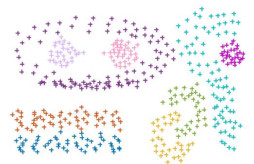
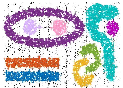
62 Single-node SGMM MR-SGMM Original Dataset s SGMM Core Points Regenerated Dataset Figure 5.5: Dataset SDS1: depictions of the original (clustered) dataset, SGMM core points and the regenerated dataset for the single-node SGMM (left column, with 269 core points) and MR-SGMM (right column, with 470 core points). Single-node SGMM MR-SGMM Original Dataset SGMM Core Points Regenerated Dataset Figure 5.6: Dataset SDS2: depictions of the original (clustered) dataset, SGMM core points and the regenerated dataset for the single-node SGMM (left column, with 358 core points) and MR-SGMM (right column, with 452 core points). 54

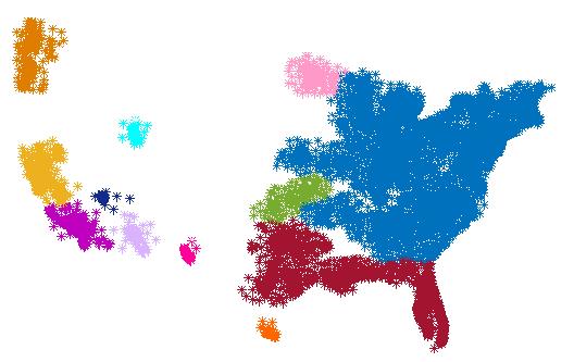
63 Single-node SGMM MR-SGMM Original Dataset SGMM Core Points Regenerated Dataset Figure 5.7: Dataset SDS3: depictions of the original (clustered) dataset, SGMM core points and the regenerated dataset for the single-node SGMM (left column, with 250 core points) and MR-SGMM (right column, with 417 core points). Single-node SGMM MR-SGMM Original Dataset SGMM Core Points Regenerated Dataset Figure 5.8: Dataset RDS1: depictions of the original (clustered) dataset, SGMM core points and the regenerated dataset for the single-node SGMM (left column, with 288 core points) and MR-S- GMM (right column, with 427 core points). 55

64 Single-node SGMM MR-SGMM Original Dataset SGMM Core Points Regenerated Dataset Figure 5.9: Dataset RDS2: depictions of the original (clustered) dataset, SGMM core points and the regenerated dataset for the single-node SGMM (left column, with 579 core points) and MR-S- GMM (right column, with 740 core points). 5.4 Figures of merit Section 5.3 showed a qualitative comparison between the single-node SGMM and MR-SGMM, indicating that MR-SGMM functions properly on a variety of datasets. However, a quantitative analysis is required to confirm these results. A common approach for examining data summarization results is to compare calculated clustering analysis measures for the original (clustered) and regenerated data. In the present research, MR-SGMM and single-node SGMM were applied to the input datasets to cluster the datasets using DBSCAN, summarize the datasets based on the SGMM core points and their variances, and finally to regenerate the datasets. Clustering analysis measures were calculated for the original (clustered) datasets and for the regenerated data, using both methods of single-node and MR-SGMM. Ideally, the difference between these clustering measures for the original data and its regenerated counterpart would approach zero to indicate quantitative similarity between regenerated and original data. 56