ΠΑΝΕΠΙΣΤΗΜΙΟ ΘΕΣΣΑΛΙΑΣ ΠΟΛΥΤΕΧΝΙΚΗ ΣΧΟΛΗ ΤΜΗΜΑ ΗΛΕΚΤΡΟΛΟΓΩΝ ΜΗΧΑΝΙΚΩΝ & ΜΗΧΑΝΙΚΩΝ ΥΠΟΛΟΓΙΣΤΩΝ

Transcription

1 ΠΑΝΕΠΙΣΤΗΜΙΟ ΘΕΣΣΑΛΙΑΣ ΠΟΛΥΤΕΧΝΙΚΗ ΣΧΟΛΗ ΤΜΗΜΑ ΗΛΕΚΤΡΟΛΟΓΩΝ ΜΗΧΑΝΙΚΩΝ & ΜΗΧΑΝΙΚΩΝ ΥΠΟΛΟΓΙΣΤΩΝ Implementation of a Distributed System for the Solution of MultiDomain / MultiPhysics Problems Ανάπτυξη Κατανεµηµένου Συστήµατος για Επίλυση Προβληµάτων Πολλαπλών - Χωρίων / Πολλαπλών - Φυσικών Μοντέλων ΔΙΠΛΩΜΑΤΙΚΗ ΕΡΓΑΣΙΑ ΚΩΝΣΤΑΝΤΙΝΟΣ Κ. ΧΑΛΚΙΑΣ Επιβλεποντες Καθηγητές: Παναγιώτα Τσοµπανοπούλου Επίκουρη Καθηγήτρια Εµµανουήλ Βάβαλης Καθηγητής Βόλος, Ιούλιος 2013

2

3 ΠΑΝΕΠΙΣΤΗΜΙΟ ΘΕΣΣΑΛΙΑΣ ΠΟΛΥΤΕΧΝΙΚΗ ΣΧΟΛΗ ΤΜΗΜΑ ΗΛΕΚΤΡΟΛΟΓΩΝ ΜΗΧΑΝΙΚΩΝ & ΜΗΧΑΝΙΚΩΝ ΥΠΟΛΟΓΙΣΤΩΝ Ανάπτυξη Κατανεµηµένου Συστήµατος για Επίλυση Προβληµάτων Πολλαπλών - Χωρίων / Πολλαπλών - Φυσικών Μοντέλων Διπλωµατική Εργασία ΚΩΝΣΤΑΝΤΙΝΟΣ Κ. ΧΑΛΚΙΑΣ Επιβλέποντες Καθηγητές: Παναγιώτα Τσοµπανοπούλου Επίκουρη Καθηγήτρια Π.Θ. Εµµανουήλ Βάβαλης Καθηγητής Π.Θ. Εγκρίθηκε από την διµελή εξεταστική επιτροπή την 5 Ιουλίου Π. Τσοµπανοπούλου Ε. Βάβαλης Επίκουρη Καθηγήτρια Καθηγητής

4

5 Διπλωµατική Εργασία για την απόκτηση του Διπλώµατος του Μηχανικού Η/Υ, Τηλεπικοινωνιών & Δικτύων του Πανεπιστηµίου Θεσσαλίας, στα πλαίσια του Προγράµµατος Προπτυχιακών Σπουδών του Τµήµατος Ηλεκτρολόγων Μηχανικών και Μηχανικών Υπολογιστών του Πανεπιστηµίου Θεσσαλίας.... ΚΩΝΣΤΑΝΤΙΝΟΣ ΧΑΛΚΙΑΣ Διπλωµατούχος Μηχανικός Η/Υ, Τηλ/νιών & Δικτύων 2013 All rights reserved

6 To my family and friends.

7 Ευχαριστίες Σε αυτό το σηµείο θα ήθελα να ευχαριστήσω όλους τους ανθρώπους που µε βοήθησαν και µε υποστήριξαν στα χρόνια σπουδών µου. Αρχικά θα ήθελα να ευχαριστήσω την επιβλέπουσα της διπλωµατικής µου εργασίας, Παναγιώτα Τσοµπανοπούλου για την εµπιστοσύνη που µου έδειξε να ασχοληθώ µε µία τόσο απαιτητική διπλωµατική εργασία. Η υποστήριξή της, η καθοδήγησή της και οι ουσιώδεις παρεµβάσεις της µε διευκόλυναν να επιτύχω την ολοκλήρωσή της. Το ενδιαφέρον της και οι συζητήσεις που είχαµε µου έδειξε ότι όχι µόνο είχαµε µια άριστη συνεργασία αλλά και ότι αναπτύξαµε µια ουσιαστική ανθρώπινη σχέση. Θα ήθελα επίσης να ευχαριστήσω τον δεύτερο επιβλέποντα της διπλωµατικής µου εργασίας κ. Εµµανουήλ Βάβαλη για τις συµβουλές του και την υποστήριξή του καθόλη τη διάρκεια των σπουδών µου. Ακόµη οφείλω ένα µεγάλο ευχαριστώ στους φίλους µου, την Αλεξία, τον Βασίλη, την Μαριάννα, τον Κώστα, την Αφροδίτη και την Χρυσή για την αγάπη τους και την υποστήριξή τους και την ανοχή τους στις ιδιοτροπίες µου όλα αυτά τα χρόνια σπουδών αλλά και κατά τη διάρκεια της εκπόνησης της διπλωµατικής µου εργασίας. Τέλος, τα εκπαιδευτικά µου επιτεύγµατα είναι το αποτέλεσµα της άνευ όρων αγάπης, υποστήριξης, ενθάρρυνσης, συµβουλής και καθοδήγησης που έχω από την οικογένειά µου. Ευχαριστώ τους γονείς µου, Ευγενία και Κυριαζή, που πάντα είναι δίπλα µου να µε στηρίζουν, να µε βοηθούν µε οποιοδήποτε τρόπο και να µου δίνουν δύναµη να συνεχίσω και να προσπαθώ για το καλύτερο δυνατό. Ακόµη θα ήθελα να ευχαριστήσω θερµά τα αδέρφια µου, Μάγδα και Περικλή, για την αγάπη τους και την κατανόησή τους. Κωστής, Βόλος, 2013

8 Περίληψη Η µοντελοποίηση και η προσοµοίωση σύνθετων φυσικών προβληµάτων περιλαµβάνει συχνά πολλά µέρη κυρίως γιατί 1. τα φυσικά προβλήµατα από µόνα τους αποτελούνται από πολλά επιµέρους υποπροβλήµατα διαφορετικής φύσης 2. οι παράλληλες υπολογιστικές στρατηγικές και προσεγγίσεις απαιτούν πολλά (σχεδών ανεξάρτητα) επιµέρους προβλήµατα, και 3. το υπάρχον λογισµό προσοµοίωσης έχει εφαρµογή µόνο σε απλά γεωµετρικά σχήµατα και µοντέλα φυσικής. Ο κύριος σκοπός αυτής της διπλωµατικής εργασίας είναι να προτείνει ένα περιβάλλον προσοµοίωσης για την επίλυση των προβληµάτων πολλαπών χωρίων / πολλαπλών φυσικών προβληµάτων µε τη µέθοδο της χαλάρωσης στις διεπαφές µεταξύ γειτονικών υποχωρίων του αρχικού προβλήµατος (Interface Relaxation). Το προτεινόµενο εργαλείο (IRTool) πρέπει να έχει αρκετές πολύ επιθυµητές ιδιότητες, όπως ευρεία εφαρµογή, αυξηµ ένη προσαρµ οστικότητα, υψηλή απόδοση, παραλληλισµό και επαναχρησιµοποίηση λογισµικού, µε την ενσωµάτωση µεθόδων σε διάφορους επιστηµονικούς τοµείς όπως η µαθηµατική ανάλυση, αριθµητική ανάλυση, oι επιστηµονικοί υπολογισµοί και οι κατανεµηµένοι υπολογισµοί.

9 Abstract The modeling and simulation of complex physical systems often involves many components because 1. the physical system itself has components of differing natures, 2. parallel computing strategies require many (somewhat independent) components, and 3. existing simulation software implies only to simpler geometrical shapes and physical situations. The main purpose of this thesis is to propose a simulation environment for solving MultiDomain / MultiPhysics problems using different relaxation methods to the interfaces between neighboring subdomains of the original problem (Interface Relaxation). The proposed tool (IRTool) should have several very desirable properties as, fast convergence, wide application, increased flexibility, high performance, parallelism and reuse of existing software, integration of the advances in various scientific fields such as mathematical analysis, numerical analysis, scientific computing and distributed computing.

10 Table of Contents List Of Acronyms 11 List of Figures 12 Chapter 1: Introduction General 16 Chapter 2: Related Works First Implementation of IR SciAgent 18 Chapter 3: Theoretical Background General Domain Decomposition & Interface Relaxation Interface Relaxation Methods The Geometric (GEO) Construction Based Method 24 Chapter 4: System Design & PDETool Matlab PDETool What does this Toolbox do? Who can use this toolbox? What Problems can I solve? In which areas can the Toolbox be used? How do I define a PDE Problem? How can I solve a PDE Problem? Can I use the Toolbox for Nonstandard problems? Who can I visualize my results? Are there any applications already implemented? IRToolbox (Interface Relaxation Toolbox) 29 10

11 4.2.1 Expanding Matlab s PDE Toolbox Architecture s Basic Idea & Functionality 29 Chapter 5: IRToolbox GUI Global Window File Menu Edit Menu Draw Menu Interface Relaxation Menu Subdomain Window Boundary Menu PDE Menu Mesh Menu 35 Chapter 6: IRTool Implementation General IRTool Initialization Geometry Decomposition Boundaries & Interfaces Interface Relaxation Graphical User Interface (GUI) 47 Chapter 7: User Guide / Numerical Experiments General Two - dimensional elliptic partial differential problem Uniform Problem - Solution Step By Step Non Uniform Problem - User Practice 53 Chapter 8: Conclusions Conclusions 55 11

12 Bibliography 56 Appendix 67 12

13 List Of Acronyms GEO AVE NEW ROB SCO SHO PDE IR PDEToolbox IRToolbox Geometric Construction Based Method A simple method of averaging the solution and its normal derivative along the interfaces. A scheme based on Newton s method to correct the interface values. An algorithm that uses Robin interface conditions for smoothing. A scheme that is based (but not formulated) on Schur complement approach. A method based on the concept of the shooting method for solving Ordinary Differential Equations (ODEs). Partial Differential Equation Interface Relaxation Partial Differential Equation Toolbox Interface Relaxation Toolbox 13

14 List of Figures Figure 2.1: The components of the SciAgent System 18 Figure 3.2.1: The Interface Relaxation mechanism 22 Figure 3.3.1: Cross section perpendicular to the interface where UL and UR have slopes SL and SR at the interface point I. Changing the values of UL and UR by a quantity m makes the slopes equal in magnitude. 24 Figure 5.1: IRTool Global Window 30 Figure 5.1.1: IRTool File Menu 31 Figure 5.1.2: IRTool Edit Menu 31 Figure 5.1.3: IRTool Options Menu 31 Figure 5.1.4: IRTool Draw Menu 31 Figure 5.1.5a: IRTool Interface Relaxation Menu 32 Figure 5.1.5b: IR Parameters pop - up window 32 Figure 5.2a: Global Window with drawn Geometry 33 Figure 5.2b: Subdomain Window for the first domain 33 Figure 5.2c: Subdomain Window for the second domain 33 Figure 5.2.1a: Boundary Menu 34 Figure 5.2.1b: Boundary Condition Window 34 Figure 5.2.1c: Interface Relaxation Condition 34 Figure 5.2.2a PDE Menu 35 Figure 5.2.2b: PDE Specification Window 35 Figure 5.2.3a: Mesh Menu 35 Figure 5.2.3b: Mesh Parameters Window 35 Figure 7.1: Matlab s Command Window 48 Figure 7.2: Geometry of the uniform problem 49 Figure 7.3: Object Dialog Window for geometry specification 49 Figure 7.4: Decomposition of the initial problem to subdomains 50 Figure 7.5: Boundary Mode of the subdomains 50 14

15 Figure 7.6: Boundary Condition Window for Uniform Problem 51 Figure 7.7: Interface Relaxation Conditions Window for Uniform Problem 51 Figure 7.8: PDE Specification Window for Uniform Problem 52 Figure 7.9: Mesh Parameters Window for Uniform Problem 52 Figure 7.10: IR Parameters Specification for uniform problem 53 Figure 7.11: Contour plot for the solution and plots for the interface relaxation of the uniform problem Figure 7.12: Contour plot for the solution and plots for the interface relaxation of the non uniform problem

16 Chapter 1: Introduction Chapter 1: Introduction 1.1 General For the numerical solution of large partial differential equations (PDE s) problems there are many techniques[1][2][11]. The first and most common approach is to discretize the geometrical domain using grids or meshes to create a large discrete problem. These grids or meshes are then partitioned to create a set of inter-connected discrete problems. This is simple Domain Decomposition (D.D. also known as sub-structuring) and the coupling between components (discrete problems) is rather tight as the mathematical model along interface points or elements is discretized into equations that involve details from both neighboring components. Moreover, domain decomposition methods solve a boundary value problem by splitting it into smaller boundary value problems on subdomains and iterating to coordinate the solution between adjacent subdomains. A coarse problem with one or few unknowns per subdomain is used to further coordinate solution between the subdomains globally. The problems on the subdomains are independent, which makes domain decomposition suitable for parallel computing. However domain decomposition methods are typically used as pre-conditioners, such as the conjugate gradient method. The second and oldest approach is Schwarz Splitting which decomposes the geometrical domain into components with small overlap[3]. In overlapping domain decomposition methods, the subdomains overlap by more than the interface. The mathematical models on each component can then be solved independently in some way and the Schwarz alternating method is applied iteratively to compute the global solution. Of course, some discretization method is applied to the solution process on each individual component. The overlapping creates a serious complication in the Schwarz method even when the global problem has a simple geometry. The method has become more feasible with the discovery of non-overlapping domain versions. The third and newest approach is Interface Relaxation (IR) where the geometrical domain is decomposed into subdomains, each with its own mathematical model. In these, non-overlapping methods, the subdomains intersect only on their interface. In primal methods, the continuity of the solution across subdomain interface is enforced by representing the value of the solution on all neighboring subdomains by the same unknown. Along the interfaces between subdomains one must satisfy interface conditions derived from the physical phenomena (e.g., continuity of mass or temperature, conservation of momentum). The models in each domain are solved in the inner loop of the interface relaxation iteration method to compute the global solution. The methods use one of a variety of smoothing formulas to reduce the error in satisfying the interface conditions. Finite element simulations of moderate size models require solving linear systems with millions of unknowns. Several hours per time step is an average sequential run time, therefore, parallel computing is a necessity. The goals of handling different physical problems, using parallel computers and reusing existing software all lead to the need for high flexibility and loose coupling between components in the computation. The approaches mentioned above have similar goals but are quite different in their generality and flexibility. The tight coupling of domain decomposition requires that neighboring components have a lot shared information about their discretizations. Further, this approach is quite awkward when the models are different on neighboring components. The mortar method creates specialized refinements of the models and meshes along the interfaces to accommodate changes in models across interfaces. overlapping Schwarz methods are similarly constraint to a single physical problem for neighboring subdomains. the non - overlapping Schwarz methods are restricted to a single mathematical model for neighboring subdomains. 16

17 Chapter 1: Introduction The interface relaxation approach imposes no coupling conditions, except those inherent in the mathematical models, and it provides maximum generality and flexibility. The interface relaxation method is the method that we are going to use in order to solve complex PDE problems. The IR methodology is an iterative procedure. First the initial problem is decomposed into smaller and simpler PDE subproblems, where there is no overlap between the neighboring subdomains. On all subdomain interface we use initial values, which we estimate. The next step is to solve each single PDE subproblem independently using the estimated values on the interfaces. If the solution that we compute is not the same as the real solution we improve the values on the interfaces using a relaxer. A relaxer is an interface relaxation method, such as GEO, ROB, AVE [12][13][14]. This procedure is progressed iteratively until satisfactory accuracy and convergence are achieved. The main purpose of this dissertation is to propose a simulation environment for solving multi-domain/multi-physics problems. More specifically we want to solve elliptic PDE problems that are coupled with both cartesian and general decompositions. The Graphical User Interface (GUI) is a simulation framework where we can draw a 2-D complicated domain and define boundary and interface conditions. We can also specify the partial differential equation, create, inspect and refine the mesh and compute the solution for the particular problem. This framework must have several very desirable properties like fast convergence, wide applicability, increased adaptivity, high efficiency, inherent parallelism and software reuse by integrating advances in different scientific areas like mathematical analysis, numerical analysis, approximation, scientific computing, distributed computing and agent computing. In the Second Chapter, we present previous related works. In the Third Chapter we provide a theoretical background about how Interface Relaxation can be used in order to solve complex PDE s problems. In the Forth Chapter a brief description of Matlab s PDETool is given. The Fifth Chapter introduces IRTool s Graphical User Interface. The PDE Toolbox is used as a base of the proposed simulating environment for the decomposition and solution with the use of various interface relaxation methods. In the Sixth Chapter we provide technical information for the implementation of our tool. In the Seventh Chapter a manual is given which provides any prospective user all the necessary guidance needed to compose the initial problem and afterwards decompose it and solve it with the Interface Relaxation Toolbox. The Eighth Chapter suggests guidelines for any future development and extension of the proposed implementation of the Interface Relaxation Toolbox. 17

18 Chapter 2: Related Works Chapter 2: Related Works 2.1 First Implementation of IR Given the fact that Methodology in Interface Relaxation is relatively new, it is easily assumable that there are only a few implementations that cover this area of research. A first but also naive of such a prototype implementation goes back to it was solely based on core TCP/IP routines to implement the collaboration among the co-workers. it did not use software parts technology but rather developed from scratch on local solvers and implemented just one relaxer. The second primitive implementation differs from the first one mainly on the fact that it exploited, based on plain KQML messages, the Agent approach to integrate the ELLPACK PSE. both were very unstable, were used through text based user interfaces, did not complied with standard technology and were very limited for our purposes [5][6][7][8][9]. Nevertheless, the later implementation have provided with a good starting point and it is presented next. 2.2 SciAgent Collaborative PDE Solvers: Theory and Practice[2], presented in 2000 an implementation of a collaborative PDE system, named SciAgent, for truly heterogeneous distributed computer systems. In particular the architecture and the main software components are described and the Agent Technology used is introduced. SciAgent implementation consists of a whole class of Interface Relaxation methods in an agent based framework that is implemented mainly using C and JAVA. This implementation is used for general two-dimensional decompositions of linear and nonlinear elliptic PDE problems. The SciAgents exploit the inherent parallelism in the interface relaxation methods using the Agents computing paradigm over a network of heterogenous workstations. The components of a SciAgent system are shown in Figure 2.1 below. Figure 2.1: The components of the SciAgent System Specifically, the SciAgents transform the physical problem into a network of local PDE solvers and interface relaxers. In the SciAgent prototype there are three types of agents: one PDECoordinator agent, several PDESolver and PDEMediator agents. The PDECoordinator, as it is Figured by its name, is responsible for the control of the entire application and coordinate the whole procedure, a PDEMediator arbitrates between the two solvers sharing a boundary between two domains, and a PDESolver is a wrapper for the legacy application and solves the local problem. 18

19 Chapter 2: Related Works When the PDECoordinator agent is started, reads a problem description file and writes the information into its model. The input file contains information about the number of solvers and mediators, the characteristics of the interfaces, the initial guesses on the interfaces, the interface relaxation methods and the names of the machines that will be used to solve the whole problem. The next step in the procedure is to create and configure the PDESolver and PDEMediator agents. The PDECoordinator uses their addresses to setup the communication between them. Then the coordinator waits for messages from the mediators, regarding the status of the convergence to the solution of the problem, or from the user. The messages from the user are to change the values of specific variables of the input file, such as convergence tolerance or to force the execution to stop. The PDESolver agent is responsible to solve the problem locally and path the input/ output files etc. In the first state, the PDESolver starts-up the Pelltool which compiles the.e file that describes the local PDE problem, and creates the executable that will be used later on by the ExecuteTool. Both Pelltool and ExecuteTool are parts of PELLPACK system. In the next state, the solver extracts the points on the interfaces from the file that contains the mesh/ grid points, and writes them into a file. Then the solver notifies the mediators that the files are ready. The PDESolver agent remains idle until being notified by the mediator that the list with all the points and their initial guesses are stored in a file at a specific location. Then the solver uses these files to run the ExecuteTool to solve the problem and then, the solver send a message to the mediators that new values are computed, and waits for their response. Depending on the message from the mediators, the solver will solve the problem again, remain idle waiting for the other solvers, or plot the local solution. The PDECoordinator is able to terminate the PDESolver by sending an appropriate message. The mediator agent, PDEMediator, is created and configured by the PDECo- ordinator agent. The mediator agent has a complete description of the interface, the relaxation method used, the solvers to collaborate with, the location of the input/ output files, the location of the legacy programs, the tolerance used to decide convergence, and the initial guess function. This information is provided by the coordinator agent. After being started, the mediator waits for the boundary points from the neighboring solvers. In the next stage, the mediator combines the two point lists and then uses the initial guess to compute values at these points. Afterwards, the mediator sends a message to the two solvers that the files with the points and their values are ready. The mediator remains idle, waiting for new values from the two solvers. When it receives new values it moves to the next stage, reads the new data and compares them with current data. Then the mediator agent uses the relaxation method to calculate the new values for the boundary conditions. If convergence is reached on this interface then the mediator sends messages to the solvers and informs the PDECoordinator about the local convergence so it will be able to decide on global convergence. A message from the coordinator is sent to the mediator and the PDEMediator will finish, in case of global convergence or wait for new data from the two solvers. SciAgents require strong interpolation support, procedure for estimating initial guesses, mechanisms for determining good values for relaxation parameters and criteria to control the iterative procedure. Interpolation is needed because grids/meshes do not necessarily match on the interface segment. Also the estimation of initial values on the interface is a very complex procedure, because the Neumman and the mixed boundary conditions are sensitive to their initial guesses and as the PDE problems get more complicated better initial guesses will be needed. 19

20 Chapter 3: Theoretical Background 3.1 General The various domain decomposition methods that have been recently developed for the efficient solution of elliptical differential equations can be easily classified into two categories - overlapping and non-overlapping [3]. Both approaches already have been used to effectively model large scale, industrial, ill-conditioned problems. Nevertheless it is believed that further theoretical and experimental analysis is required before such methods will become practical and useful tools for non - experts. Overlapping (Schwarz) schemes have received in the past a great deal of attention. Articles that review and compare various such schemes and survey the associated preconditioning strategies have already appeared in the literature. it is relatively recent that a number of studies have shown that non-overlapping schemes can compete well an d can possibly free the user from certain complications in their formulation and implementation. the comparison of the main characteristics of these two classes of methods and the existence of equivalent relations between them have already received a great deal of study. Interface relaxation methods takes us a step beyond non overlapping domain decomposition. In an effort to mimic the physics in the real world, they split a complicated partial differential equation (PDE) that acts on a large and / or complex domain into a set of PDE problems with different but simple operators acting on different and easy to solve subdomains. This Multi - PDE, Multi - Domain system is properly coupled using smoothing operations on the inter domain boundaries. From the interface relaxation viewpoint, the methods that can be used in order to solve a problem, consist of partitioning the domain on a set of non-overlapping subdomains and of imposing some boundary conditions on the interface boundaries defined by this partition. Then, using initial guesses on the interfaces, the set of the resulting PDE problems is solved. The solutions obtained do not satisfy the interface boundary conditions and interface relaxation is applied to obtain new interface boundary values, which satisfy the conditions better, and we solve the PDEs with these new values. We repeat the above steps until the desired convergence is acquired. For this dissertation we have collected most of the known interface relaxation methods and for the implementation of the IRTool we have used the GEO method. Specifically, we consider the methods listed below in alphabetical order with respect to their acronyms. These acronyms are used in the sequel to refer to associated methods. AVE A simple method of averaging the solution and its normal derivative along the interfaces. GEO A method based on a simple geometric contraction. NEW A scheme based on Newton s method to correct the interface values. ROB An algorithm that uses Robin interface conditions for smoothing. SCO A scheme that is based (but not formulated) on Schur complement approach. Chapter 3: Theoretical Background SHO A method based on the concept of the shooting method for solving Ordinary Differential Equations (ODEs). 20

21 Chapter 3: Theoretical Background SPO A method originated from the use of Steklov Poincare operator which involves alternating boundary condition types. 3.2 Domain Decomposition & Interface Relaxation The domain decomposition world consists of two parts, overlapping and non-overlapping. Overlapping, known also as Schwarz, methods were the first considered and have already proved themselves as very efficient numerical procedures enjoying certain very desirable convergence properties. Nevertheless, it has been also observed that they might have serious drawbacks which will prohibit their use for certain applications. For example, almost all of the many proposed domain decomposition methods for solving wave propagation models (that consist of the Helmoltz equation coupled with various absorbing or reflecting boundary conditions) are non-overlapping. Non overlapping methods exhibit certain advantages compared to overlapping ones. Specifically: They are not sensitive to jumps on the operator coefficients. Their convergence behavior and theoretical errors estimates remain the same even if the differential operator includes discontinuous coefficients provided that the jumps occur along the interface lines. They have smaller communication overhead in a parallel implementation on distributed memory multiprocessor systems. Their communication overhead is proportional to the length of the interface lines while it is proportional to the overlapping are in the case of overlapping methods. The bookkeeping is rather easy for the decomposition and manipulations of the associated data structures compared to the more complicated and costly bookkeeping of the overlapping methods. Interface relaxation is a step beyond non overlapping domain decomposition; it follows Southwell s relaxation of the 1930 but at the PDE instead of the linear algebra level - to formulate relaxation as iterated interface smoothing procedures. A complex physical phenomenon consists of a collection of simple parts with each one of them obeying a single physical law locally and adjusting its interface conditions with neighbors. Interface relaxation partitions the domain on a set of non overlapping subdomains, imposes some boundary conditions on the interface among subdomain lines. given an initial guess, it imitates the physics of the real world by solving the local problems exactly on each subdomain and relaxing boundary values to get better estimates of correct interface conditions. The procedure described above can be explained as an algorithm, as follows : 1. Guess solution values (and derivatives if needed) on all subdomain interfaces. 2. Solve all single PDEs exactly and independently on all the subdomain with these values as boundary conditions. 3. Compare and improve the values on all interfaces using a relaxer 4. Return to Step 2 until satisfactory accuracy is achieved. The simplest relaxers do some sort of smoothing of values on the interfaces and averaging is a good mental model for a relaxation formula. 21

22 Chapter 3: Theoretical Background Figure 3.2.1: The Interface Relaxation mechanism The illustrated Figure above shows the generic relaxation formula Gij (based on the current solutions Ui new and Uj new of the two local to the neighboring subdomains Ωi and Ωj ) calculates successive approximations bi,j New to the solution on the interface Γi,j between them. To formally describe this method we consider the differential problem (3.1) where D is an elliptic, non-linear in general, differential operator and B a condition operator defined on the boundary δω of an open domain Ω E R d, d=1,2,... This domain is partitioned into p open subdomains Ωi,i=1,...,p such that (3.2) For reasons related either to the physical characteristics of this problem or to the computing resources available, one would like to replace (3.1) with following system of loosely coupled differential problems (3.3) 22

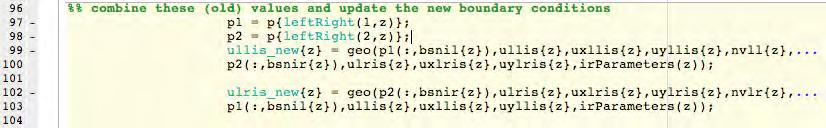
23 Chapter 3: Theoretical Background where i=1,...,p. These differential problems are coupled through the interface conditions Giju=0 and involve the restrictions Di and Bi of the global differential and boundary operators, D and B, respectively, on each subdomain with some of them possibly linear and some other nonlinear. The functions fi and ci are similar restrictions of the function f and c. The local interface operator Gij is associated with the interface relaxation method and different selections for the Gij s lead to different relaxation schemes. In this dissertation we consider interface relaxation methods that have the following characteristics. They first decompose the problem (3.1) at differential level and then discretize the resulting differential subproblems (3.3). They have the versatility to use the most appropriate discretization scheme for each subproblem. They do not overlap the subdomains Ωi using good relaxation parameters in Gi, they are fast enough so no preconditioning is needed. They simplify the geometry and physics of the computation by considering the subproblems (3.3) instead of the global differential problem (3.1). They can utilize software parts technology by reusing existing legacy software parts for solving the individual subproblems (3.3). They are general and robust. 3.3 Interface Relaxation Methods Due to the inherent abstraction, it is relatively easy to describe the various interface smoothing methods at both the conceptual and algorithmic level. For the purpose of this dissertation though, we will present only the GEO method which is used for the implementation of our tool. For simplicity in the presentation of algorithms, we consider only one way (along the x axis) partition of the domain. Therefore each subdomain can have at maximum two interface lines with the two neighbouring subdomains. The basic building block for our algorithm is the procedure u = solve_pde(ui,dui) which calculates the solution u of the local to a subdomain PDE problem with Dirichlet, Neumann or GEO boundary conditions on the interface using as the interface values ui and its gradient dui. The subscripts R and L denote left and right subdomains or interfaces respectively and ui denotes the solution of the problem associated with subdomain Ωi. 23

24 Chapter 3: Theoretical Background Figure 3.3.1: Cross section perpendicular to the interface where UL and UR have slopes SL and SR at the interface point I. Changing the values of UL and UR by a quantity m makes the slopes equal in magnitude The Geometric (GEO) Construction Based Method GEO estimates the new solution for each subdomain by solving a Dirichlet problem and is classified as an one step method. The values on the interfaces are obtained by adding to the old ones, a geometrical weighted combination of the normal boundary derivatives of the adjacent subdomains. Specifically, we assume in Figure that UL and UR are the solutions of the PDE problems associated with the left and right subdomains, respectively, of the interface point I. They are equal along interface I and we denote by SL and SR their slopes at I. As it can be easily seen geometrically, m is the correction needed to be added to UL and UR so as to match the normal derivatives I. To calculate m we consider the two triangles IAB and CDI whose heights are given by multiplying the corresponding tangent with the base of the triangle, or equivalently by multiplying the normal derivative with the base. The bases wl and wr are the widths assumed for the validity of the slope values; these can be arbitrary selected and play the role of the relaxation parameters. The new interface values are now given by adding the weighted average of the heights to the old interface values UL and UR. One can intuitively view this as grabbing the function U at the I and stretching it up by m until its derivative becomes continuous. numerical experiments show that the convergence rate does not seem to depend much on the widths wl and wr. In case that UL and UR are not equal on I we simply use their average. GEO is given algorithmically by 24

25 Chapter 4: System Design & PDETool Chapter 4: System Design & PDETool 4.1 Matlab PDETool What does this Toolbox do? The Partial Differential Equation (PDE) Toolbox [4] provides a powerful and flexible environment for the study and solution of partial differential equations in two space dimensions and time. The equations are discretized by the Finite Element Method (FEM). The objectives of the PDE Toolbox are to provide you with tools that: Define a PDE problem, i.e., define 2-D regions, boundary conditions, and PDE coefficients. Numerically solve the PDE problem, i.e., generate unstructured meshes, discretize the equations, and produce an approximation to the solution. Visualize the results Who can use this toolbox? The PDE Toolbox is designed for both beginners and advanced users. The minimal requirement is that you can formulate a PDE problem on paper (draw the domain, write the boundary conditions, and the PDE). Start MATLAB. At the MATLAB command line type: pdetool This invokes the graphical user interface (GUI), which is a self-contained graphical environment for PDE solving. For common applications you can use the specific physical terms rather than abstract coefficients. Using pdetool requires no knowledge of the mathematics behind the PDE, the numerical schemes, or MATLAB. Advanced applications are also possible by downloading the domain geometry, boundary conditions, and mesh description to the MATLAB workspace. From the command line (or M-files) you can call functions from the toolbox to do the hard work, e.g., generate meshes, discretize your problem, perform interpolation, plot data on unstructured grids, etc., while you retain full control over the global numerical algorithm What Problems can I solve? The basic equation of the PDE Toolbox is the PDE (c u)+au = f in Ω, which we shall refer to as the elliptic equation, regardless of whether its coefficients and boundary conditions make the PDE problem elliptic in the mathematical sense. Analogously, we shall use the terms parabolic equation and hyperbolic equation for equations with spatial operators like the one above, and first and second order time derivatives, respectively. Ω is a bounded domain in the plane. c, a, f, and the unknown u are scalar, complex valued functions defined on Ω. c can be a 2- by-2 matrix function on Ω. The toolbox can also handle the parabolic PDE 25

26 Chapter 4: System Design & PDETool the hyperbolic PDE and the eigen value problem where d is a complex valued function on Ω, and λ is an unknown eigenvalue. For the parabolic and hyperbolic PDE the coefficients c, a, f, and d can depend on time. A nonlinear solver is available for the nonlinear elliptic PDE (c(u) u) + a(u)u = f(u), where c, a, and f are functions of the unknown solution u. All solvers can handle the system case (c 11 u 1 ) (c 12 u 2 ) + a 11 u 1 + a 12 u 2 = f 1 (c 21 u 1 ) (c 22 u 2 )+a 21 u 1 +a 22 u 2 = f 2. You can work with systems of arbitrary dimension from the command line. For the elliptic problem, an adaptive mesh refinement algorithm is implemented. It can also be used in conjunction with the nonlinear solver. In addition, a fast solver for Poisson s equation on a rectangular grid is available.the following boundary conditions are defined for scalar u: Dirichlet: hu = r on the boundary Ω. Generalized Neumann: n (c u) + qu = g on Ω. n is the outward unit normal. g, q, h, and r are complex valued functions defined on Ω. (The eigenvalue problem is a homogeneous problem, i.e., g = 0, r = 0.) In the nonlinear case, the coefficients, g, q, h, and r can depend on u, and for the hyperbolic and parabolic PDE, the coefficients can depend on time. For the two-dimensional system case, Dirichlet boundary condition is h11u1 + h12u2 = r1 h 21 u + h 1 22 u 2 = r, 2 the generalized Neumann boundary condition is n (c 11 u 1 )+n (c 12 u 2 )+q 11 u 1 +q 12 u 2 = g 1 n (c 21 u 1 )+n (c 22 u 2 )+q 21 u 1 +q 22 u = g 2 2, 26

27 Chapter 4: System Design & PDETool and the mixed boundary condition is h 11 u + h u = r n (c 11 u 1 )+n (c 12 u 2 )+q 11 u 1 +q 12 u 2 = g 1 +h 11 µ n (c 21 u 1 )+n (c 22 u 2 )+q 21 u 1 +q 22 u 2 = g 2 +h 12 µ, where µ is computed such that the Dirichlet boundary condition is satisfied. Dirichlet boundary conditions are also called essential boundary conditions, and Neumann boundary conditions are also called natural boundary conditions In which areas can the Toolbox be used? The PDEs implemented in the toolbox are used as a mathematical model for a wide variety of phenomena in all branches of engineering and science. The following is by no means a complete list of examples: The elliptic and parabolic equations are used for modeling steady and unsteady heat transfer in solids flows in porous media and diffusion problems electrostatics of dielectric and conductive media potential flow The hyperbolic equation is used for transient and harmonic wave propagation in acoustics and electromagnetic transverse motions of membranes The eigenvalue problems are used for, e.g., determining natural vibration states in membranes and structural mechanics problems Last, but not least, the toolbox can be used for educational purposes as a complement to understanding the theory of the Finite Element Method How do I define a PDE Problem? The simplest way to define a PDE problem is using the graphical user interface (GUI), implemented in pdetool. There are three modes that correspond to different stages of defining a PDE problem: Draw mode, you create Ω, the geometry, using the constructive solid geometry (CSG) model paradigm. A set of solid objects (rectangle, circle, ellipse, and polygon) is provided. You can combine these objects using set formulas. In Boundary mode, you specify the boundary conditions. You can have different types of boundary conditions on different boundary segments. In PDE mode, you interactively specify the type of PDE and the coefficients c, a, f, and d. You can specify the coefficients for each subdomain independently. This may ease the specification of, e.g., various material properties in a PDE model. 27

28 Chapter 4: System Design & PDETool How can I solve a PDE Problem? Most problems can be solved from the graphical user interface. There are two major modes that help you solve a problem: In Mesh mode, you generate and plot meshes. You can control the parameters of the automated mesh generator. In Solve mode, you can invoke and control the nonlinear and adaptive solvers for elliptic problems. For parabolic and hyperbolic problems, you can specify the initial values, and the times for which the output should be generated. For the eigenvalue solver, you can specify the interval in which to search for eigenvalues. After solving a problem, you can return to the Mesh mode to further refine your mesh and then solve again. You can also employ the adaptive mesh refiner and solver. This option tries to find a mesh that fits the solution Can I use the Toolbox for Nonstandard problems? For advanced, nonstandard applications you can transfer the description of domains, boundary conditions etc. to your MATLAB workspace. From there you use the functions of the PDE Toolbox for managing data on unstructured meshes. You have full access to the mesh generators, FEM discretizations of the PDE and boundary conditions, interpolation functions, etc. You can design your own solvers or use FEM to solve subproblems of more complex algorithms Who can I visualize my results? From the graphical user interface you can use Plot mode, where you have a wide range of visualization possibilities. You can visualize both inside the pdetool GUI and in separate Figures. You can plot three different solution properties at the same time, using color, height, and vector field plots. Surface, mesh, contour, and arrow (quiver) plots are available. For surface plots, you can choose between interpolated and flat rendering schemes. The mesh may be hidden or exposed in all plot types. For parabolic and hyperbolic equations, you can even produce an animated movie of the solution s time-dependence. All visualization functions are also accessible from the command line Are there any applications already implemented? The PDE Toolbox is easy to use in the most common areas due to the application interfaces. Eight application interfaces are available, in addition to the generic scalar and system (vector valued u) cases: Structural Mechanics - Plane Stress Structural Mechanics - Plane Strain Electrostatics Magnetostatics AC Power Electromagnetics Conductive Media DC Heat Transfer Diffusion 28

29 Chapter 4: System Design & PDETool These interfaces have dialog boxes where the PDE coefficients, boundary conditions, and solution are explained in terms of physical entities. The application interfaces enable you to enter specific parameters, such as Young s modulus in the structural mechanics problems. Also, visualization of the relevant physical variables is provided. Several nontrivial examples are included in this manual. Many examples are solved both by using the GUI and in command-line mode. The toolbox contains a number of demonstration M-files. They illustrate some ways in which you can write your own applications. 4.2 IRToolbox (Interface Relaxation Toolbox) Expanding Matlab s PDE Toolbox The PDE Toolbox is written using MATLAB s open system philosophy. There are no blackbox functions, although some functions may not be easy to understand at first glance. The data structures and formats are documented. Anyone can examine the existing functions and create his / her own as needed Architecture s Basic Idea & Functionality The IRTool (Interface Relaxation Tool) is a Matlab Toolbox that solves MultiDomain MultiPhysics Problems. Firstly we studied PDETool which as mentioned before solves 2 - Dimensional PDE problems. Although PDETool can face multi-domain problems at the linear algebra level of study (domain decompositions techniques), it is not able to solve multidomain multiphysics problems with Interface Relaxation (IR) Methods. The common boundary between different domains of a PDE problem, named interfaces, can be treated as the physics demand in a high level of decomposition by the IR methodology. We embedded PDEtool in our toolbox, IRTool, in order to be able to define multiphysics / multidomain PDEs, set appropriate conditions on the global boundary, define/call proper methods on the interfaces, solve the global problem and visualize the solution of the entire PDE problem. Our work was quite difficult since we had to understand the MATLAB code, find out the proper data structures the MATLAB uses to store and compute a PDE problem and then use them properly in our toolbox to define and solve a composed PDE problem by making multiple PDETools communicating properly, which in PDETool case it does not allow us to create more than one design window. 29

30 Chapter 5: IRToolbox GUI Chapter 5: IRToolbox GUI 5.1 Global Window The PDE Toolbox which is implemented in Matlab provides a flexible environment for the study and solution of partial differential equations. Nevertheless, it does not handle with interface relaxation methods the common boundaries of a multi domain problem. This is the reason that inducts us to implement the IR Toolbox. The Interface Relaxation Toolbox provides a graphical user environment for the study and solution of partial differential equations with multiple domains / multiple physics as it considers at the same time the interface relaxation methodology. Therefore, the IRToolbox has some additional properties and capabilities. The basic need was that with the IRTool we can deal with the interface segments and solve the global problem by contemplating parameters such as interface relaxation method, initial guesses on the interface segments and tolerance for the convergence of the global solution. The Graphical User Interface (GUI) of IRTool is an extension of PDETool s GUI with some modifications that are implied by the IR methodology. IR has a pull-down menu bar that we can use to control the modeling. It conforms to common pull-down menu standards. Menu items followed by a right arrow lead to a submenu. Menu items followed by an ellipsis lead to a dialog box. Standalone menu items lead to direct action. Some menu items can be executed by using keyboard accelerators. IRTool also contains a toolbar with icon buttons for quick and easy access to some of the most important functions. The following sections describe the contents of IRTool menus, the dialog boxes associated with menu items and an illustrated example. To get started with the graphical environment we simply type in the Matlab prompt the command irtool. The GUI looks like the Figure below (Figure 5.1) and is the initial / global window of our implementation. Figure 5.1: IRTool Global Window 30

31 Chapter 5: IRToolbox GUI File Menu The pull-down menu has the following applications: New, Open, Save, Save As, Print, Exit. These applications deal with basic procedures that exist in many toolboxes of Matlab Edit Menu The Edit menu provides the applications below: Undo, Cut, Copy, Paste, Clear, Select All Options Menu Similarly, the Options menu is the same as the pull-down Options menu of the pdetool. Its applications are: Grid, Grid spacing, Snap, Axis Limits, Axis Equal, Turn off Toolbar Help, Zoom, Application and Refresh. Figure 5.1.1: IRTool File Menu Figure 5.1.2: IRTool Edit Menu Figure 5.1.3: IRTool Options Menu Draw Menu In the Draw Mode, we can draw the geometry on which we want to solve the PDE. As in PDE Toolbox, the IRTool provides four types of solid objects: polygons, rectangles, circles, and ellipses by the selecting the following options from the pulldown menu of the Draw menu: Rectangle/Square, Rectangle/square (centered), Ellipse/Circle, Ellipse/Circle (centered), Polygon. In order to rotate the selected objects we can use the Rotate choice from the same menu. The objects are used to create a Constructive Solid Geometry model (CSG model). Each solid object is assigned a unique label, and by the use of set algebra, the resulting geometry can be made up of a combination of unions, intersections, and set differences. By default, the resulting CSG model is the union of all solid objects. The only thing that we must take care when we draw the geometry is that the solid objects must not overlap each other if we want to solve the PDE problem using the interface relaxation methodology. Figure 5.1.4: IRTool Draw Menu 31

32 Chapter 5: IRToolbox GUI Interface Relaxation Menu Interface Relaxation Menu in the global window provides us with the following two choices A. Decompose Geometry Splits the initial geometry to the consisting subdomains. Each subdomain is redrawn to individual window - subdomain window - awaiting for further specification, i.e. boundary conditions, interface relaxation conditions e.t.c. B. Parameters Opens additional window for user entry. The user has to specify the number of iterations that the interface method will execute and the error tolerance (convergence). The window by default has the iteration number set to 20 and the error value set to 0.5e-6. C. Solve MultiPDE Starts the solution of all the subdomains & interfaces. D. Clear IR Parameters In case that we want to insert new boundary values,pde coefficients e.t.c. we have first to choose this menu in order the old parameters to be flashed out from our subdomains. Figure 5.1.5a: IRTool Interface Relaxation Menu Figure 5.1.5b: IR Parameters pop - up window 5.2 Subdomain Window Supposing that we have the initial / global geometry shown in Figure 5.2a, pressing the Decompose geometry from the Interface Relaxation menu, the current geometry splits in multiple windows -subdomain windows-. Every window now creates a unique handle for every subdomain as shown in Figures 5.2b and 5.2c respectively. 32

33 Chapter 5: IRToolbox GUI Figure 5.2a: Global Window with drawn Geometry Figure 5.2b: Subdomain Window for the first domain Figure 5.2c: Subdomain Window for the second domain Boundary Menu In the Boundary menu we have the following options:boundary mode, Specify Boundary Conditions, Show Edge Labels, Show Sub-domains Labels, Remove Sub-domain Border, Remove All Sub-domain Borders and Export Decomposed Geometry, Boundary Cond s, as shown in Figure 5.2.1a. 33

34 Chapter 5: IRToolbox GUI Figure 5.2.1a: Boundary Menu We can now define the boundary conditions for the outer boundaries but for the interfaces as well. We can enter the Boundary Mode by clicking the Ω icon, or by selecting Boundary Mode from the Boundary menu. The boundaries are indicated by colored lines with arrows. The boundary condition can also be a function of x and y, or simply a constant. By default, the boundary condition is of Dirichlet type: u = 0 on the boundary. If we double click on a boundary segment the boundary condition window pops up as shown in Figure 5.2.1b Figure 5.2.1b: Boundary Condition Window If we double click on an interface then the interface condition window pops up as presented in Figure 5.2.1c. In this window the user can insert the initial condition of the interface which can be a vector, a function or even another Matlab file which contains an expression that can be evaluated. The default interface relaxation method is GEO. There is also an option for a user define method. In this case the user has to create his / her own IR method. Figure 5.2.1c: Interface Relaxation Condition PDE Menu The PDE menu is exactly as it is in Matlab and has the following options as shown in Figure 5.2.2a: PDE Mode, Show Sub-domain Labels, PDE Specification and Export PDE Coefficients. The parameter d does not apply to the elliptic PDE. The coefficients a, c and f can be constants or 34

35 Chapter 5: IRToolbox GUI functions. In order to specify the PDE equation and its coefficients for each subdomain we have to choose PDE Specification and enter the desired values in the window as shown in Figure 5.2.2b. Figure 5.2.2a PDE Menu Figure 5.2.2b: PDE Specification Window Mesh Menu The Mesh menu has the following options: Mesh Mode, Initialize Mesh, Re- fine Mesh, Jiggle Mesh, Undo Mesh Change, Display Triangle Quality, Show Node Labels, Show Triangles Labels, Parameters and Export Mesh as is presented in the Figure 5.2.3a. Parameters for controlling the jiggling of the mesh, the refinement method, and other mesh generation parameters can be found in a dialog box that is opened by selecting Parameters from the Mesh menu. At this time, we must initialize the maximum edge number, as this refers to the hmax. Hmax is necessary in order to solve the PDE problem. This menu is the same as it is in PDE Toolbox and the window that appears looks like the Figure 5.2.3b. Figure 5.2.3a: Mesh Menu Figure 5.2.3b: Mesh Parameters Window 35

36 Chapter 6: IRTool Implementation Chapter 6: IRTool Implementation 6.1 General In this chapter we are going to give further information about the implementation of IRToolbox. Since PDETool as has already been mentioned is open source we had to alter some of it s files in order to achieve the desirable result. We also had to create a few new files also to implement IRToolbox. The created files with all the code that has been written can be found at the end of this thesis in the appendix. 6.2 IRTool Initialization One of the first changes that we had to make in Matlab s PDETool was its ability to open more than one window since only one at a time can be open. Since our primal problem has to be decomposed in many other, IRTool must support this functionality. As already presented in the previous chapter IRTool has a main / global window in which we draw the initial problem, and thereafter our toolbox decomposes it to each subproblems / subdomains. The files that were created are 1. irtool.m It contains the function irtool() which simply calls the pdetool() function. This function was created to avoid writing pdetool() in order to initialize our toolbox. So in order ti initialize our tool we have to type irtool() The file that we altered was 1. pdetool.m When pdetool is called with no input arguments it calls the pdetool( initialize ) which draws the initial window. Before the drawing of the window we inserted the following lines of code. It was also necessary to insert the global variable pde_fig which is used in almost every file which denotes at every given time the current IRTool window. 6.3 Geometry Decomposition Once the user has drawn the geometry that describes his / her problem, he / she can then choose Decompose Geometry from the Interface Relaxation menu of the main / global window. When the user chooses to decompose the initial / global geometry then the function pdetool( decomposegeometry ) is called. This function is an addition to pdetool.m file as another else - if statement for the kind of function that our toolbox wants to execute. The number of lines and the code of this block of code is presented bellow. 36

37 Chapter 6: IRTool Implementation In this if -else branch two other functions all called which are also inside the pdetool.m file. 1. pdetool( ir ) This function finds the boundaries and the interfaces that every subdomain has. This is a necessary step before the decomposition of the geometry, since PDETool would ignore the interface segments. In this part of the development we had to introduce another global variable - a cell array - called splitgometryincellarray which contains the decomposed geometry of every subdomain.the produced code is shown below 2. pdetool( split ) In this code block the subdomain windows are created, since the geometry of every subdomain is now known by the previous function. At this part becomes more obvious the importance of the global variable pde_fig and the few lines of code that we inserted in the beginning of pdetool.m 37

38 Chapter 6: IRTool Implementation In the above code block pdeinit.m is called which is actually responsible for the kind of the initialization that happens. In PDEToolbox if there is not an opened window, this functions calls pdetool.m to create one. If there is an active window and pdeinit.m is called then it clears the current window. We had to change this function so that our tool will not clear the initial geometry but open another window. In the following code inside pdeinit.m we added lines

39 Chapter 6: IRTool Implementation 6.4 Boundaries & Interfaces Once the user has decomposed his / her geometry can enter boundary mode. We had to make a few modifications in this part too in order for the interfaces to appear in this mode. If we had not make the changes presented below our toolbox would handle interfaces as common boundaries. The changes we made in some existing files and the new files we created are the following: Changes 1. pdetool('drawbounds') This function is called within pdetool( boundmode ). The decomposed geometry description matrix that PDETool creates for every subdomain contains information for all the line segments that consist a boundary / interface. The first row contains the type of segment, if it is a line,circle,ellipse segment. The next four lines contain information about the coordinates of each segment. The sixth and seventh lines contain information about the left and right hand region of each segment. This piece of information is vital for us. PDETool denotes the wide external region of a domain with zero. If both these lines are not both equal with zero means that is an interface. The additions / changes that we introduced are shown below. 39

40 Chapter 6: IRTool Implementation 2. pdetool( initbounds ) It is called within pdetool( drawbounds ) and packs and initializes the boundary and interface conditions. 3. pdetool(interfaceclk) It is another code block inside pdetool.m that makes us able to double click with the mouse on an interface in order to insert interface conditions. 40

41 Chapter 6: IRTool Implementation 4. pdetool( set_internal_bounds ) Its called from pdetool(interfaceclk) and is responsible for preparing the interface to acquire the input that the user enters - pack and unpack parameters-. 41

42 Chapter 6: IRTool Implementation New file created 1. irbddlg.m This function designs and handles the interface boundary condition window that appears when the user double clicks with his / her mouse on an interface line. The code implementation of this function can be found in the appendix. 6.5 Mesh Initialization One other change that we had to make in order our toolbox to work properly is the mesh production strategy. Once the initial geometry has been decomposed to component subdomains the mesh generation of each geometry changes. This is forced by the fact that since each subdomain is single on each window it does not have at the left / right hand region in the decomposed geometry matrix one or more segments with other neighboring subdomain / subdomains. So if we proceed to create the mesh for each subdomain, a wrong one will be produced. In order to achieve the correct mesh initialization we had to alter the function pdemgeom.m which is called from the function initmesh.m that starts the mesh creation. Specifically after the decomposition of each subdomain we search which line segments have a left / right hand region that is not the same with the internal region of the current subdomain. Once this region is found is set to zero. This change of values is not saved in the decomposed geometry matrix-is only used for the triangulation. The code block that has been added to pdemgeon.m is 42

43 Chapter 6: IRTool Implementation 6.6 Interface Relaxation The last stage of the development of our toolbox was the implementation of the interface relaxation method. At this stage appeared any other file modifications that we had to implement and also the creation of many new functions. Due to the fact that all the files that were created were extensive in code lines here we will present only the line codes of interfacerelaxation.m function as long as the functionality of all the functions that are called by it. The implementation of those functions can be found in the Appendix. Firstly we had to add a few lines of code in the pdetool.m function in order to make the menu Solve MultiPDE responsive and functional. Additionally we had to implement also the functionality of the pop up window for the user input of iteration number and error for the interface relaxation methodology. 43

44 Chapter 6: IRTool Implementation Once the user has finished entering all the necessary variables of his / her problem can start the solution of the problem by pressing the Solve MultiPDE choice from the Interface Relaxation Menu on the main / global window. This action calls the interfacerelaxation.m function which is presented below 44

45 Chapter 6: IRTool Implementation 45

46 Chapter 6: IRTool Implementation Inside the interfacerelaxation function the following functions are being called: 1. subdomaininfo.m Gathers all the specifications and variables that we inserted for each subdomain, such as IR parameters, IR initial condition, the line segments in which an interface exists e.t.c., 2. initmesh.m Builds an initial triangular PDE mesh 3. createmesh.m Creates a cartesian mesh 4. correctboundfile.m After the extraction of the interfaces initial conditions it replaces them with irleft or iright according to whether the current interface is in the left or right hand region of the domain under inspection 5. solvedomains.m Solves the domain in order to get the new value for every iteration 46

47 6. tri2cartmesh.m Computes uc and its derivatives (Uxc and Uyx) on the cartesian 7. interfinfo.m Given a mesh of a domain, find out information for a specific boundary segment. This information is valuable for the IR methodology. 8. interfvalues.m Computes the function and its derivatives on the interface points 9. geo.m computes the new values of u on the interface nodes of each domain relaxing the old values from both neighboring domains using the outward normal vector. Chapter 6: IRTool Implementation 6.7 Graphical User Interface (GUI) Last but not least we had to make some changes in the initial and the subdomain window layout. These changes concern if a menu button is available at any stage of the problem modeling procedure. The changes were made in the pdetool.m file and are inflicted in lines We present here only the code block for the Interface Relaxation menu which was not implemented in PDEToolbox. 47

48 Chapter 7: User Guide / Numerical Experiments Chapter 7: User Guide / Numerical Experiments 7.1 General! The purpose of this chapter is to demonstrate and verify the functionality of IRTool by experimentally examining its validity. For this dissertation we have implemented the GEO method for elliptic problems using IRTool we restricted our experiments to partitions in two or three subdomains. 7.2 Two - dimensional elliptic partial differential problem Uniform Problem - Solution Step By Step For this let us consider the following elliptic problem: Lu(x,y) 2 u(x,y)+γ 2 u(x,y)=f(x,y), (x,y) Ω u(x, y) = u b (x, y), (x, y) Ω, The true solution u(x,y) is u(x,y) = e y(x+4) x(x-1)(x-0.9)y(y-0.5). This PDE problem consists of a geometry that is decomposed into three domains with interfaces on x1 = 1/3 and x2 = 2/3, Hmax =0.05 and omega is 0.03 and 0.04 for the first and second interface respectively. In order to initialize IRTool we type irtool in Matlab s command window. Figure 7.1: Matlab s Command Window 48

49 Chapter 7: User Guide / Numerical Experiments Automatically IRTool enters Draw Mode. In this stage the user has to draw the physical problem. One can either use the Draw Menu or the buttons below the menu in order to determine what type of geometry his / her problem consists of. Figure 7.2: Geometry of the uniform problem In order to achieve maximum accuracy for our domains we can double click on any subdomain and manually insert the coordinates, height and width of each one. The window that appears is shown below Figure 7.3: Object Dialog Window for geometry specification Once the desired geometry is designed we choose Decompose Geometry form the initial / global window. This action leads to the decomposition of the initial geometry to subdomains. 49

50 Chapter 7: User Guide / Numerical Experiments Figure 7.4: Decomposition of the initial problem to subdomains There after it is time to enter boundary mode for each subdomain, so we choose Boundary Mode from the Boundary Menu for each subdomain. Figure 7.5: Boundary Mode of the subdomains In Boundary Mode by double click on each boundary or interface we can give the input according to our problem. The two Figures below show the user input for both boundaries and interface according to the initial description of the problem. 50

51 Chapter 7: User Guide / Numerical Experiments Figure 7.6: Boundary Condition Window for Uniform Problem Figure 7.7: Interface Relaxation Conditions Window for 1st Interface Figure 7.8 Interface Relaxations Conditions for 2nd Interface Afterwards we insert PDE Parameters for each domain from the PDE Menu. At this stage IRTool has entered PDE Mode. 51

52 Chapter 7: User Guide / Numerical Experiments Figure 7.8: PDE Specification Window for Uniform Problem Following the Menu from the main / global window we then must specify the hmax for the generation of the mesh in each subdomain. For our problem we use as input for mesh parameters as maximum edge size 0.05 (hmax =0.05) as shown in the Figure Figure 7.9: Mesh Parameters Window for Uniform Problem Before we proceed to the solution of our problem we have to specify the number of iterations and error value from the menu IR Parameters from the main / global window. 52

53 Chapter 7: User Guide / Numerical Experiments Figure 7.10: IR Parameters Specification for uniform problem The modeling of our problem is now complete. Lastly we have to choose Solve MultiPDE from the Interface Relaxation Menu in the main / global window. The Figure below shows the contour of the solution and the relaxation in each of the two interfaces. Figure 7.11: Contour plot for the solution and plots for the interface relaxation of the uniform problem during the 25th iteration Non Uniform Problem - User Practice The second PDE problem consists of a geometry that is decomposed into three domains with interfaces on x1 = 1/5 and x2 = 1/2. We use the same differential elliptic equation and true solution u(x,y), as we used in For further practice the reader can model the problem him / herself. Below is the Figure of the solution. 53

54 Chapter 7: User Guide / Numerical Experiments Figure 7.12: Contour plot for the solution and plots for the interface relaxation of the non uniform problem during the 29th iteration 54

55 Chapter 8: Conclusions 8.1 Conclusions We propose an implementation of IRToolbox for composite PDE problems by properly combining existing models and software components. Our approach enjoys the following approaches: Problem simplification. It dramatically simplifies the complexity of the physical problem by (1) considering subproblems that involve simpler local physical rules acting on simpler geometries, and (2) providing a convenient abstraction of the modeling and solution process while simultaneously providing a modeling practice that yields a closer representation of the physical world. Reduction in software development time. It drastically reduces the time to develop a simulation engine by permitting the heavy reuse of legacy scientific software. Numerical efficiency. It increases the efficiency of the overall numerical scheme by allowing one to reuse the most appropriate numerical method for each particular subproblem. This thesis focuses on the implementation of IRToolbox that consists one proposal for solving MultiDomain / MultiPhysics Problems. 55

56 Bibliography 1] A. Quarteroni, A. Valli. Domain decomposition methods for partial differential equations. Oxford University Press, [2] Panagiota Tsompanopoulou, Collaborative PDE Solvers: Theory and Practice. PhD Thesis, University of Crete, Department of Mathematics, [3] P.E. Bjorstad, O. Widlund, To overlap or not overlap: A note on a domain decomposition method for elliptic problems (Pages: ) [4] PDE Toolbox, Matlab, [5] H.S. McFaddin. An Object-based Problem Solving Environment for Collaborating PDE Solvers and Editors., PhD Thesis, Computer Science Department, Purdue University, [6] T.T. Drashansky, An agent-based approach to building multidisciplinary problem solving environments. PhD Thesis, Computer Science Department, Purdue University, [7] T.T. Drashansky, E.N. Houstis, N. Ramakrishnan, J.R. Rice, Networked Agents for Scientific Computing. ACM Communications, [8] S.Karin, S.Graham, The high performance computing continuum., ACM Communications, [9] T.Finin, Y.Labrou, J.Mayfield, KQML as an agent communication language. Cambridge, [10] S.McFaddin, J.R. Rice, RELAX: A software platform for PDE Interface Relaxation methods.csd-tr , [11] J.R. Rice, P.Tsompanopoulou, E.Vavalis, Interface relaxation methods for elliptic differential equations. Applied Numerical Mathematics 32 (2000) , Purdue University, Computer Science Department, [12] J.R. Rice, P.Tsompanopoulou, E.Vavalis, Fine Tuning interface relaxation methods for elliptic differential equations.technical Report CSD-TR , Purdue University, Computer Science Department, [13] Analysis of an Interface Relaxation Method for Composite Elliptic Differential Equations, P. Tsompanopoulou and E. Vavalis, Journal of Computational and Applied Mathematics, 226(2), (Apr. 2009), pp [14] An Experimental Study of Interface Relaxation Methods for Composite Elliptic Differential Equations, P. Tsompanopoulou and E. Vavalis, Applied Mathematical Modelling, 32, (Aug. 2008), pp

57 Appendix Initialization 1. irtool.m Boundary 1.irbddlg.m i 67

58 Appendix 68

59 Appendix 69

60 Appendix 70

61 Appendix 71

62 Appendix 72

63 Appendix 73

64 Appendix 74

65 Appendix 75

66 Appendix 76

67 Appendix 77

68 Appendix 78

69 Appendix 79

70 Appendix Interface Relaxation 1. subdomaininfo.m 80

71 2.initmesh.m Panagiota Tsompanopoulou All rights reserved 3.correctBoundFile.m i 67

72 Appendix 4.solveDomains.m 68

73 Appendix 69

74 Appendix 70

75 Appendix 71

76 Appendix 72

77 Appendix 5. tri2cartmesh.m Panagiota Tsompanopoulou All rights reserved 6.interfinfo.m Panagiota Tsompanopoulou All rights reserved 73

78 Appendix 7.interfvalues.m - Panagiota Tsompanopoulou All rights reserved 74