BAYESIAN SEGMENTATION OF THREE DIMENSIONAL IMAGES USING THE EM/MPM ALGORITHM. A Thesis. Submitted to the Faculty.

Transcription

1 BAYESIAN SEGMENTATION OF THREE DIMENSIONAL IMAGES USING THE EM/MPM ALGORITHM A Thesis Submitted to the Faculty of Purdue University by Lauren Christopher In Partial Fulfillment of the Requirements for the Degree of Doctor of Philosophy May 2003

2 - ii - In memory of Ann Whitman Christopher, my mother.

3 - iii - ACKNOWLEDGMENTS Thanks to Dr. Charles Meyer and Dr. Paul Carson of the Department of Radiology at the University of Michigan, Ann Arbor, Michigan, for the medical data and their explanations and assistance. Thanks also to my thesis committee, Dr. Delp, Dr. Bouman, Dr. Babbs, and Dr. Zoltowski, for their guidance. Thanks for the love and support of my husband, Dave Duffield, and for the love of my children Ann and Christina.

4 - iv - TABLE OF CONTENTS Page LIST OF FIGURES vi ABSTRACT ix 1 Introduction Overview and Problem Statement Literature Overview Summary of our Contributions Bayesian Approaches: EM/MPM, EM/MAP-ICM and EM/MAP-SA Algorithms Definitions Statistical Models of X, 2-D and 3-D Cliques, and Markov Random Fields Statistical Model of Y X, and Bayesian estimation of X Y MAP-ICM Algorithm MAP-SA Algorithm MPM Algorithm New Attenuation Compensation Expectation-Maximization EM Convergence Criteria Initialization Experimental Results MAP-ICM, MAP-SA, and MPM Algorithm Comparison EM/MAP-ICM Algorithm Summary EM/MAP-SA algorithm summary EM/MPM algorithm summary

5 - v Test Images Results Initialization Results Sensitivity Results Test Image Results, Noise with Attenuation Breast Ultrasound Results CT Results Natural Images and Video Results Summary and Future Research APPENDIX A.1 Ultrasound Data LIST OF REFERENCES VITA

6 - vi - LIST OF FIGURES Figure Page 2.1 The Bayesian Model Pixel Clique in 3D Ultrasound Source Image, Frame 45 and Results Effect of Gamma Test Image Results Result of Poor Initialization Class Simplification, MPM Algorithm Effect of β on Segmentation of 2D Images Effect of M on Segmentation of 2D Images Test Image with SNR=3 and Attenuation, Algorithms Comparison Number of Class Labels using MPM Variable Mean and Gamma Ultrasound Case 175T Comparison of 3D and 2D Segmentation, Variable Mean and Gamma Compensation for EM/MPM Case 173 Original and Segmentation Result Case 173, 3D data Visualization, Target Class Isolated Segmentation Error, Case Image Difficult Cases Clinician Assistance, Case Difficult Cases Using Assisted Manual Segmentation Case 109 assisted hand segmentation D CT Images: Original Image and Segmented Image, Convergence Reached at p = Frames of Volume CT Images: Original

7 - vii D CT Images: 2 Frames of 2D EM/MPM D CT Images: Center 2 of 7 Frame 3D EM/MPM Girl Image, 7 Class Labels House Image, 7 Class Labels Girl-Office, 7 Class Labels D vs. 2D Salesman, 7 Class Labels A.1 Case 175T A.2 Case 173T A.3 Case A.4 Case A.5 Case A.6 Case A.7 Case A.8 Case A.9 Case A.10 Case 109, two slices A.11 Case 117, two slices A.12 Case 118, two slices A.13 Case 118b A.14 Case 119, three slices A.15 Case A.16 Case 121, two slices A.17 Case A.18 Case A.19 Case A.20 Case A.21 Case A.22 Case A.23 Case 88, two slices

8 - viii - A.24 Case A.25 Case A.26 Case A.27 Case A.28 Case A.29 Case A.30 Case 95b, two hand segmentations A.31 Case A.32 Case

9 - ix - ABSTRACT Christopher, Lauren. Ph.D., Purdue University, May, Bayesian Segmentation of Three Dimensional Images Using the EM/MPM Algorithm. Major Professor: Edward J. Delp. Medical images such as ultrasound, Computed Tomography (CT) and Magnetic Resonance Imaging (MRI) are typically acquired in three-dimensional (3D) volumes. In addition to true volumetric imaging, sequentially acquired images can be used to form 3D volumes using registration techniques. However, noise and distortion adversely effects clinical interpretation. This is particularly true for medical images such as ultrasound, which have speckle noise caused by reflections and variations in attenuation throughout the tissue structures. A key clinical need is to isolate parts of the 3D volume for interpretation. This requires 3D segmentation to separate tissue types and highlight abnormalities. In practice, very experienced clinicians are needed to accurately diagnose a difficult ultrasound image. Any assistance to this process is beneficial, such as automatic or semi-automatic segmentation. Segmentation using Bayesian techniques on the 2D images are not cohesive when rendered and viewed as volumes. These methods are also not adequate for segmenting the difficult ultrasound cases. Therefore, new 3D Bayesian algorithms are needed. Most 3D Bayesian algorithms find the Maximum a posteriori (MAP) estimate with the iterated conditional mode (ICM) algorithm. This algorithm can be easily trapped in local minima, especially in noisy images. In contrast, the Minimization of Posterior Marginals (MPM) algorithm determines a more appropriate solution in a large range of cases. In addition, the MPM solution provides a robust estimate of the posterior marginal probability used to find an estimate of the Gaussian model statistics used in the Expectation-Maximization (EM) algorithm.

10 - x - In this thesis, a new algorithm is described which extends the combined EM and MPM framework to 3D by including pixels from neighboring frames in the Markov Random Field (MRF) clique. In addition, the adverse attenuation in ultrasound and other medical images is addressed with a new approach that includes a unique linear cost factor introduced in the optimization and a Gaussian posterior distribution with variable mean.

11 INTRODUCTION 1.1. Overview and Problem Statement Three-dimensional (3D) medical imaging has enjoyed wide application in the last decade due to advanced visualization techniques and improved computational cost. Ultrasound, Computed Tomography (CT) and Magnetic Resonance Imaging (MRI) data typically are acquired in 3D volumes. This is done by capturing successive 2D frames along a third axis, by moving the subject or the transducer. Recently an ultrasound volumetric image scan obtained by a single transducer array has been reported [1]. The application of Vibro-Acoustic imaging techniques has been shown in [2] to detect small (110 micron) microcalcification structures in breast ultrasound. However, the best application of 3D and 2D imaging can be hampered by noise and other image processing problems. These limitations are particularly true for ultrasound images, which have speckle noise caused by reflections of the sound wave and variations in attenuation through the tissue structures. An ultrasound image is composed by measuring the timing of (corresponding to the depth of) the sound wave echo signal. The image is built by the reflection of these waves from tissues and tissue boundaries. Images acquired in a time sequential manner can also be composed into volumes. The work in [3, 4, 5, 6] has allowed 3D volumes to be viewed from 2D image sequences. This work also includes solutions to the registration problem for multiple images. However, a major key to clinical interpretation of 3D images is segmentation. Today, much of the segmentation is done by hand in isolated 2D slices. Automatic or semi-automatic segmentation in 3D is an open research problem in medical image

12 - 2 - processing research. Years of experience are needed to provide a clinical interpretation of ultrasound images. Several major effects combine to cause difficulties. The characteristic speckle noise of ultrasound data is caused by the off-axis reflections of the sonic wave in variable density tissue. In addition, there is strong attenuation of the signal corresponding to the depth of the tissue to be imaged. This attenuation effect is further degraded as higher frequency ultrasound is used to obtain a better spatial resolution. Finally, the capture of ultrasound is prone to problems with the transducer/skin interface and the difficulty illuminating the object of interest. In this thesis we will address the noise and attenuation effects with an algorithm which has better performance than the current literature. We will use several 3D ultrasound volume sets obtained at the University of Michigan Department of Radiation, which has been compounded and registered by the algorithms in [3, 4, 6]. Ultrasound images are among the most difficult to segment. Standard segmentation techniques such as filtering, region growing, thresholding, and non-linear edge operations are minimally effective in ultrasound images because of the high noise and attenuation degradation. For CT and MRI images the attenuation and noise effects are less severe, however a statistical approach may be quite beneficial for these volumes as well. Segmenting ultrasound can be viewed as a texture segmentation problem. The preferred segmentation technique for these textured images is based on statistical modeling of the distribution of the pixels and the statistical character of the noise. Besag [7] and Geman and Geman [8] pioneered a statistical framework for image processing. The technique they proposed assumes a hidden model that is distorted by a statistical process to form the observed image. A key idea in the technique is the assumption of a statistical model for the hidden image. Bayes rule then can be used to separate the observed data described by a joint probability distribution into a conditional distribution and a marginal (prior) distribution. The hidden model is known as the prior distribution because a priori knowledge is used. A model is also

13 - 3 - needed for the process that distorts the data. A model of the hidden data and the model of the distortion process together are used to statistically infer the posterior distribution. The solution which maximizes this posterior distribution is known as the MAP (maximum a posteriori) estimate. Finding the MAP estimate analytically is not feasible, so iterative optimization algorithms are required to maximize this distribution (also called the objective function). A mathematical tutorial of three MAP segmentation algorithms is provided in Chapter 2. The first is Iterated Conditional Modes (MAP-ICM), which is a steepest descent maximization algorithm. The second is Simulated Annealing (MAP-SA) which contains a Monte-Carlo randomization. The third is Maximization of Posterior Marginals (MPM) which also uses the Monte-Carlo method, but has an important side benefit, discussed in Chapter 2. For all three algorithms, a Markov Random Field (MRF) is used as the prior model of the hidden image. This forces the constraint of a neighborhood system which models the spatial interaction of the underlying image and tissues, and provides the framework for convergence (to a local maximum). As is typical, the neighborhood system used in this thesis is defined by the nearest spatial locations. For 2D the system is the four rectilinear compass points, and for 3D we add the two pixels co-located in the adjacent slices (images). To find a Bayesian segmentation, we must also know or infer several statistical parameters. The model of the distortion contains unknown statistics, (the mean and variance of an assumed Gaussian model). As a group, we will call these hyperparameters. The method for determining these hyper-parameters varies. In our research, we estimate the hyper-parameters using Maximum Likelihood (ML) methods, specifically the Expectation-Maximization (EM) algorithm. In Chapter 2 we provide details of the EM algorithm. Additionally, the prior model needs the actual or estimated probability of the various segmentation classes (e.g. tumor, background, and tissue). One contribution of our research, to be described in Chapter 2, is to provide a new way of modeling the distortion and finding the associated statistics, as well as adapting the segmentation

14 - 4 - class probability to compensate for the distortion in ultrasound. In our research we form the problem as a joint estimation problem (hyper-parameter estimation and MAP estimation of the segmentation classes) and propose to solve the problem using an iterated approach. Specifically, we use EM finding the ML estimate of the hyperparameter estimation, and compare three MAP iterative optimization algorithms as the maximization part of EM. This creates a nested loop structure with the following two steps which are repeated until convergence: E-Step: Estimate the hyper-parameters using the results of a MAP segmentation, forming the outer loop. M-Step: Estimate the segmentation classes using one of three MAP algorithms, holding constant the hyper-parameters estimated in the E-Step, thus forming the inner loop Literature Overview Selected applications of 2D Bayesian techniques for texture segmentation are found in the following references. A multiscale segmentation technique is described in [9] which performs a MAP segmentation of the wavelet coefficients of the image, each coefficient taken in turn, and each result of the low frequency coefficients are passed as initializations for the higher frequency coefficients. A multiscale pyramid-filtered image segmentation is presented in [10]. In [11] an application of Bayesian segmentation to functional brain MRI images is described. The work in [12] uses a combined MAP-ICM and the Expectation-Maximization (EM) algorithm for segmenting brain MRI. Described in [13] is a multiscale application of MAP-ICM techniques to isolate lesions in breast ultrasound images. Some interesting recent papers [14, 15] use a combination of MAP and MPM, where MAP-ICM finds an initial segmentation, and then MPM is used to refine it. Multiresolution MPM algorithms [16, 17] find a segmentation at a lower resolution which is used as the initialization for the full

15 - 5 - resolution segmentation, this improves the result, particularly with noisy or high variance images. These techniques all describe a solution to the maximum a posteriori (MAP) segmentation problem in different ways. The hyper-parameter estimation is done either with a priori knowledge or with a variety of algorithms. The next set of papers describe Bayesian segmentation algorithms on 3D image data. A multi-resolution MAP-ICM segmentation for 3D data for in vivo cardiac ultrasound is shown in [18]. The hyper-parameters are estimated using textural (entropy, contrast, correlation) and acoustic (mean central frequency and integrated backscatter) features. In [19] a 3D MRF segmentation is performed on MRI images. Simulated annealing is used to converge to the best segmentation (in the MAP sense). Another 3D segmentation is described in [20] of Brain MR images with training to obtain the hyper-parameters, with the comparison of two algorithms, simulated annealing (SA) and Iterated Conditional Modes (ICM). A comparison of the MAP-SA, MAP-ICM, and MPM algorithms was described in [21] with the conclusion that MAP-ICM was considered the most robust with Signal to Noise Ratio (SNR) = 1. In contrast, in this research we show that MAP-ICM is trapped in local maxima for SNR < 1, whereas the MPM and MAP-SA algorithms perform well through SNR < 0.5. At SNR < 0.5, the MAP-SA algorithm produces a single segmentation class as the maximization, while the MPM continues to perform well until SNR = 0.4. We also note that the initialization may be responsible for the results shown in this paper. This thesis extends the work described in [17, 16], combining the EM algorithm for hyper-parameter estimation and the Maximization of Posterior Marginals (MPM) algorithm for the segmentation. The benefit of MPM as described in [22] is an improved localized solution to the segmentation when compared with the MAP-ICM estimate. MPM assigns a cost to the number of incorrectly classified pixels, rather than optimizing for an overall average. In addition, when MPM is used in the M-step, it can provide posterior marginal probability estimates for the EM hyper-parameters. The combined EM/MPM proof of convergence is given in [17]. We compare EM/MPM

16 - 6 - to two algorithms which combine EM with one of two MAP segmentations, ICM or SA. For MAP-ICM and MAP-SA a less accurate estimate of the posterior marginals is used in the EM update equations, as described in Chapter 2. As described in [18], there is an additional problem in ultrasound images. The attenuation across the (2D) image corresponding to the depth of the scan distorts the resulting image. A MAP estimation technique to estimate the distortion and obtain the segmentation in ultrasound was reported [23]. A recent paper [24] describes 3D segmentation of Brain Magnetic Resonance Images (MRI) using a MAP-MPM algorithm using a membrane spline function to address the MRI intensity bias field. This paper is the most similar to our work in the use of MPM as the M-Step, and the way the bias field estimation is done Summary of our Contributions Described in our recent papers [25, 26], we use several new ideas to address attenuation and noisy images. First we use a cost factor inside the MAP estimation (M-step), which has the effect of modifying the prior probabilities across the image, compensating for the attenuation (or bias). This method has the advantage of employing the optimization in the attenuation compensation. We combine this with a similar modification to the model of the posterior distribution which significantly improves the segmentation result and convergence. In this thesis we also show the application of this idea to MAP, and perform a quantitative comparison of the MAP vs. MPM segmentation for 32 test case volumes in Chapter 3. The importance of our research results is most dramatic in the ultrasound breast images. We are able to obtain a reasonably accurate segmentation on some very difficult images. The majority of the segmentation improvement comes from our new combined attenuation compensation approach. No other research to date has employed modifications to both the prior model statistics and the distortion (Gaussian) model statistics. Another important conclusion is the result of the comparison of the

17 - 7 - segmentation optimization strategies. We see EM/MPM as a superior solution for low signal to noise cases such as ultrasound. If clinician data is available a priori, an improved assisted segmentation result is shown using our algorithm. Chapter 2 describes the three 3D statistical approaches: the EM/MPM, EM/MAP- ICM and EM/MAP-SA algorithms, all with the use of the new attenuation compensation for ultrasound. Additionally the description of the hyper-parameter initialization strategy is given. Chapter 3 provides a comparison using test and real images of the three algorithms, with further experimental results shown with ultrasound, CT, natural images and video sequences. A summary of our research is provided in Chapter 4.

18 BAYESIAN APPROACHES: EM/MPM, EM/MAP-ICM AND EM/MAP-SA ALGORITHMS This chapter describes three Bayesian algorithms for segmenting image volumes: Expectation-Maximization / Maximization of Posterior Marginals (EM/MPM), Expectation- Maximization / MAP Iterated Conditional Modes (EM/MAP-ICM), and Expectation- Maximization / MAP Simulated Annealing (EM/MAP-SA). The EM algorithm is consistently used in these joint estimation technique, and is described in Section 2.8. We also describe our new extensions needed for attenuation compensation in Section 2.7. We begin the chapter with definitions and a statement of the Bayesian Maximum a posteriori (MAP) problem. The goal of Bayesian segmentation is to infer an underlying source image from a corrupted observed image, given a priori knowledge. In the case of medical imaging, we want to separate tissue types given a distorted observation. For this we use knowledge of the tissue structure and of the distortion that is typical of the image acquisition technology. To achieve this goal, we will use statistical methods to iteratively find the locally optimal segmentation, given a model of the data and optimization criteria Definitions In this thesis, the observed, gray-level image values in a 3D volume are modeled as a vector of continuous random variables, Y. A particular 3D volume is Y = y, where y is a 3D matrix containing the observed data pixels. The underlying true segmentation is denoted as X and is also a vector of random variables. Each pixel in X belongs to one of a set of discrete segmentation classes, or class labels, k {1, 2,, N}, where

19 - 9 - Fig The Bayesian Model N is the number of classes and is assumed to be known. X is therefore modeled as a vector of discrete random variables. A particular X = x, where x is a 3D vector of actual class labels. In our research, the probability mass function, p X (X = x), is the Bayesian prior probability distribution. We can model the observation process as shown in Figure 2.1. The prior data is passed through an additive noise process, and the output is the observed data. Our goal is to find an estimate of x, given the observed data y, we will denote this estimate as x. Let the set S be the set of all locations in a sampling grid in the 2D or 3D volume, where s represents a single pixel location, (x, y, z), in S. So, for example, Y s corresponds to a continuous random variable of observed data at a particular 2D or 3D location. The parameter vector, θ = (µ 1, σ1, 2 µ 2, σ2, 2, µ N, σn 2 ), contains the statistics, means and variances, of the mixture probability density function, f(y X). Here we assume conditionally independent random variables, and N is the number of classes, as described above. In addition, we assume the observed gray-level values, y given x, are independent and identically distributed (iid) Gaussian random variables (one of N Gaussian distributions) for each pixel in S. These assumptions are reasonable in most cases, however as we see for ultrasound, a modification is needed to the Gaussian model to better represent the observed images. Since the class labels, or segmentation, cannot be found analytically, three iterative algorithms will be used to estimate x. The parameters in θ are estimated using the

20 EM algorithm, while the MAP estimation algorithm is used to determine the estimate of x, ˆx. We shall denote these estimates as x MP M, x MAP SA or x MAP ICM. The p-th EM iteration determines the maximum likelihood estimate of θ, denoted ˆθ(p). These two steps are repeated until convergence is reached: E-Step: Estimate the Gaussian parameters ˆθ(p), given x(p), using the EM algorithm M-Step: Find a new x(p + 1), given ˆθ(p), using one of three MAP optimization strategies Statistical Models of X, 2-D and 3-D Cliques, and Markov Random Fields Since X is a vector of discrete random variables, a prior statistical model of X must be obtained which models the behavior of the image and is consistent with the use of Bayesian methods. The Markov Random Field (MRF) defined below is a well developed model [27, 8] incorporating the spatial dependency in images. The MRF is formed from a pixel clique C and a probability mass function. Our 2D pixel clique is defined mathematically as: and the 3D pixel clique as : C (x,y) = (X (x 1,y), X (x+1,y), X (x,y+1), X (x,y 1) ). (2.1) C (x,y,z) = (X (x 1,y,z), X (x+1,y,z), X (x,y+1,z), X (x,y 1,z), X (x,y,z+1), X (x,y,z 1) ). (2.2) These are shown in Figure 2.2. To differentiate between the two systems, we will define a pixel location (x, y, z) as 3s, and location (x, y) as 2s, correspondingly C 2s = C (x,y), and C 3s = C (x,y,z). Where both cliques are valid, we will just use s. The 2D and 3D boundary conditions are truncated, therefore, and a reduced pixel clique is used, for example, the corners have only two neighbors for 2D or four neighbors for 3D.

21 Fig Pixel Clique in 3D A clique, C, is defined as a symmetric neighborhood system of pixels. For every pixel s S, s is not in the clique, and if r is a neighbor of s, then s is a neighbor of r. This symmetry allows the Markov property to be used. The Markov property uses a Markov Chain made of M successive estimates of X, ˆx(1), ˆx(2)..., ˆx(M). The Markov property (Markov-1) states that each new estimate of X, denoted ˆx(t), is independent of any earlier estimates greater than 1 neighboring estimate: p(ˆx(t) x(t 1) = p(ˆx(t) ˆx(t 1), ˆx(t 2)...). The Markov property enables the separability of each estimate of x, allowing parallel, independent updating of the pixels s in S. The Markov Random Field (MRF) then is a class of stochastic processes where the conditional probability of neighboring sites has the clique symmetry defined in Equation 2.3. Also, any MRF random process is uniquely determined by these conditionals. If r is one of the clique locations with respect to s we have: P (X s = x s X r = x r, (r s)) = P (X s = x s X r = x r, X r C) s S. (2.3) By the Hammersley-Clifford theorem [8], if the probability mass function of X is of the form of a Gibbs distribution, then the system is a MRF. The Gibbs distribution is defined as: p X (x) = P (X = x) = 1 Z exp [r,s] C βt(x s, x r ) r C γ xr (2.4)

22 where: 0 x r = x s ; t(x s, x r ) = 1 x r x s. (2.5) In Equation 2.4, Z is a normalizing value, β is the weighting factor which, if larger, increases the amount of spatial interaction in the probability mass function. An important parameter in our research is γ xr, the cost factor for class x r = k used for modeling a non-uniform class label probability. This is important for attenuation compensation and for modeling the spatial probabilities of the class labels, as we will see in Section 2.7. Increasing γ xr for a class label k will decrease the proportion of class k in the solution. This is equivalent to modifying the relative prior probabilities of the class labels. The advantageous use of this is described in [25] and in Section Statistical Model of Y X, and Bayesian estimation of X Y We first assume that the random variables in the observed vector Y, conditioned on X, are independent. Second, any random variable Y s is assumed to be only dependent on the corresponding X s from the class label field. Thirdly we assume the distribution f Y X (y x) can be modeled with statistics vector, θ = (µ 1, σ1, 2 µ 2, σ2, 2, µ N, σn 2 ) where N =number of classes. In Equation 2.6, x s takes on the class value k {1, 2,, N}. In this research, we assumed that f Y X (y x) are independent, identically distributed (iid) Gaussian probability density functions. This gives a joint probability density function (also known as the likelihood function) of: f Y X (y x, θ) = s S { } 1 exp (y s µ xs ) 2 2πσ 2 xs 2σx 2 s (2.6) Now we use Bayes rule, combining Equations 2.4 and 2.6, to find the probability mass function p X Y (x y, θ):

23 p X Y (x y, θ) = f Y X(y x, θ)p X (x) f Y (y θ) = 1 Zf Y (y θ) s S 1 exp 2πσ 2 xs This posterior distribution, p X Y (y s µ xs ) 2 2σ 2 x s [r,s] C βt(x s, x r ) r C (2.7) γ xr = (x y, θ), is also a Gibbs distribution and a likelihood function. Our segmentation solution is the choice of x which maximizes this posterior distribution, p X Y = (x y, θ), this is the MAP estimate, x. This cannot be accomplished analytically, therefore we will use iterative optimization techniques. The function to be maximized is the posterior distribution. However, the exponential is a monotonically increasing function, so we can equivalently maximize the log p X Y and ignore the terms that do not depend on x, namely 1 Zf Y (y θ). Maximum a posteriori (MAP) optimization equation: x MAP = arg max x s S log σ x s (y s µ xs ) 2 2σ 2 x s [r,s] C βt(x s, x r ) r C This yields the γ xr (2.8) Three approaches can be used to construct this estimate. We define an objective function: U(x) = s S log σ x s (y s µ xs ) 2 2σ 2 x s [r,s] C βt(x s, x r ) r C γ xr (2.9) In the next three sections, we use this objective function U(x) to examine three maximization algorithms commonly used in the literature; MAP-SA [8], MAP-ICM [27], MPM [22], and a comparison of the three [21]. These three algorithms estimate x given the parameter vector θ. The estimation of θ is described in Section MAP-ICM Algorithm Besag [27] described a method of optimizing U(x) in Equation 2.9 by maximizing each term of the sum independently, allowable because the Markov property holds as

24 in Section 2.2. This is known as Iterated Conditional Modes (ICM). This corresponds to maximizing for each pixel (or voxel for 3D) of the s S, with a given x r, scanned in arbitrary order. We will define this pixel based objective function as u s : With: x s:map ICM = arg max x s S x r {u(x s x r, θ)} (2.10) u(x s x r, y s, θ) = log σ xs (y s µ xs ) 2 βt(x 2σx 2 s, x r ) γ xr (2.11) s [r,s] C r C A few iterations through the volume are required to converge the algorithm to a solution. This is a greedy algorithm, which successively chooses the class value x s = k which maximizes u. This algorithm is also known to become trapped in locally optimal solutions. This can be a significant problem for noisy images as we see in our tests. Once the algorithm converges, typically when the change in the objective function u is less than a threshold value, we then want to find θ given our segmentation result. There are many ways to find these parameters [12, 28]. We will use the Expectation- Maximization algorithm, of which the segmentation is the maximization or Mstep. For the EM update equations, we need an estimate of probability distribution of the underlying data p(x y), as is seen in Section 2.8. For MAP-ICM, there is no direct estimate for this distribution. Here we have used an idea similar to [22] in which we use the proportion of iterations that x s (t) = k as an estimate of the probability p Xs Y (k y, θ), where k is the class label assigned by the maximization of u(x s x r, y s, θ). The index t is defined as the iteration number t 1, 2,..., M, to M, the maximum. This estimate of the probability distribution is not theoretically robust for ICM, since the greedy strategy is not guaranteed to converge in distribution to p Xs Y (k y, θ), although in practice the estimate is reasonable. General MAP convergence is assured due to the Markov property and the ICM algorithm s choice of maximum solution at each spatial location and each iteration [27].

25 MAP-SA Algorithm The Simulated Annealing optimization problem is defined in [8]. Here the optimization of U(x) is performed using a Monte-Carlo technique. This algorithm exploits the equivalence of the Markov Random Field and the Gibbs distribution. As in [8], we use a Gibbs sampler to choose class label x s = k. Let us define a uniform, (0, 1], random variable ξ, and further define a conditional distribution given in Equation 2.12 containing the objective function. This equation includes the normalizing constant Z to form a valid distribution. Additionally we define an annealing temperature, T = f(t) = 3, where the f(t) defines the annealing schedule with respect to the log(1+t) iteration number t 1, 2,..., M, as suggested in [8]. π Xs Y (x s x r, y s, θ) = 1 { } 1 Z exp T u(x s x r, y s, θ) (2.12) The Gibbs sampler can be expressed as: if (ξ < π 1 ) then x s = class label 1 (2.13) if (π 1 < ξ < π 1 + π 2 ) then x s = class label 2 if (π 1 + π 2 < ξ < π 1 + π 2 + π 3 ) then x s = class label 3. This Gibbs sampler can be updated independently at each spatial location, due to the Markov property as in the ICM case. Each iteration at site s provides an estimate x smap SA. Each iteration decreases the annealing temperature, in our case from 4.3 to 0.76, as t increases from 1 to 50. Early in the annealing schedule, the x s is more likely to be replaced with a random choice of class, then at T = 1, x s is replaced by a particular class with probability equal to the posterior marginal distribution, and late in the annealing schedule, x s tends to remain in its previous state. For determining ˆθ in the EM equations, detailed in Section 2.8, we again use the proportion of iterations that x s = k as an estimate of the probability p Xs Y (k y, θ), where k is the class label of ˆXs optimization. This only converges in distribution for

26 T = 1. When T is varied, this proportion provides a better estimate of the marginal probability than in the ICM case, although it is not theoretically robust. Here again the general MAP convergence is assured by the construction of the Gibbs sampler, annealing schedule, and Markov property [8] MPM Algorithm In order to show the comparison between the MAP estimator and MPM, it has been shown [14] that if we model MAP using a cost factor where the cost is zero for the correct solution, and is one for an incorrect solution: C MAP (x, x) = 1 δ(x x) (2.14) then Equation 2.8 is equivalent to minimizing the expected value of C over x, with Ω =state space of x: arg min E {C MAP (x, x)} = C MAP (x, x) ( p X Y (x y, θ) ) dx (2.15) x x Ω MAP estimation assigns the same unit cost, independent of the number of erroneous pixels. This can lead to a globally optimal solution, which for high noise situations, will reduce the segmentation accuracy locally. In contrast, the MPM algorithm uses a cost function that is proportional to the number of pixels that are in error. Segmenting an image by the MPM algorithm, given some fixed θ, is performed by minimizing the expected value of misclassified pixels. This technique is shown in [16, 22, 14] to be equivalent to maximizing P (X s = x s Y = y), the posterior marginal distribution. Here we introduce the cost function: C MP M (x, x) = (1 δ(x s x s )) (2.16) s S we want to minimize the expected value of the cost, where S =number of pixels in the data set. Using the discrete form:

27 arg min E {C MP M (x, x)} = x x k C MP M(x, x) ( p X Y (x y, θ) ) = x k s S (1 δ(x s x s )) ( p X Y (x y, θ) ) = S ( s S {x:x s = x s } px Y (x y, θ) ) (2.17) since S is fixed, this function will be minimized if the second term is maximized. This brings us to the maximization of posterior marginals: x MP M = arg max x s S {x:x s=k} ( px Y (x y, θ) ) (2.18) and with respect to each pixel location s, these probabilities can be maximized independently. To find the optimal class labels, over all s, MPM maximizes each pixel with respect to: arg max x {x:x s =k} p X Y (x y, θ) = arg max p Xs Y (k y, θ). (2.19) x Where p Xs Y (k y, θ) is the posterior marginal distribution at a pixel location s, therefore we are Maximizing Posterior Marginals. No direct solution of Equation 2.19 is feasible since the probability of a single spatial sample given some 3D observation (X s Y ) is intractable. Therefore, an estimate is found using a Gibbs sampling iterative algorithm, similar to the MAP-SA algorithm. For MPM, the Gibbs sampler chooses class label x s = k by using the uniform random variable ξ, using the local posterior distribution of X s : p Xs Y (x y, θ) = 1 exp s S 2πσ 2 xs (y s µ xs ) 2 βt(x 2σx 2 s, x r ) s [r,s] C r C The Gibbs sampling becomes: γ xr (2.20) if (ξ < p 1 ) then x s = class label 1 (2.21) if (p 1 < ξ < p 1 + p 2 ) then x s = class label 2 if (p 1 + p 2 < ξ < p 1 + p 2 + p 3 ) then x s = class label 3.

28 Each iteration of the Gibbs sampler at site s is a valid estimate, x smp M. Separation of the product terms (sum terms inside exponential) is again possible using the Markov property. This algorithm is equivalent to MAP-SA with constant T = 1 annealing temperature. The Gibbs sampler is used to create a Markov Chain X(t), where the iteration number is t {1, 2,, M} and M is the number of MPM iterations. In the limit, the fraction of iterations which X(t) spend in class label k will converge in distribution to p Xs Y (k y, θ). However, here the proportion of iterations that x s = k forms a robust estimate of the posterior marginal probability p Xs Y (k y, θ). This theoretically robust sample probability is used again in the E-Step of EM, for determining ˆθ, as seen in Section 2.8. As shown in [17] the general convergence, using the EM/MPM algorithms, of the joint estimation of θ and x is proven New Attenuation Compensation This section describes the modifications for improved results when using any of the three statistical segmentation algorithms, although the best results are found with EM/MPM. As seen in Figure 2.3, and as reported in the literature [23], segmentation algorithms for ultrasound have the additional burden of finding the optimal solution across an image with a severe brightness variation. Partial compensation for this brightness variation is done at the hardware level, and our source image data includes this compensation. With traditional segmentation of ultrasound, we see in Figure 2.3(b), the attenuation causes the target and the background to be merged, both shown in black. We need to find a way to separate the target class from background and compensate for the attenuation in ultrasound. Our attenuation compensation has three interlocking ideas. First we compensate for the attenuation in ultrasound by modifying the Gaussian formulation in the posterior distribution in Equation 2.6. A function is defined, making each Gaussian mean a function of the spatial position as reported in our recent work [26]. For the ultrasound case we use a linear function fit to the data in a minimum mean squared

29 Fig Ultrasound Source Image, Frame 45 and Results (a) Ultrasound image with hand segmented data (b) EM/MPM Segmentation, no Compensation error (MMSE) sense. We have the following; µ xs = f(s) = ms + b (2.22) where s is the 3D spatial position, and m and b are vectors of the 3D slope and intercept. The MMSE estimates m and b from the data are defined as m and b, respectively, and the algorithm is defined in Section 2.8. Of course, other models of mean variation can be used. A membrane spline function for the mean [24] has been proposed for MRI data, using a MAP estimate of the spline parameters. By contrast, our algorithm embeds the function of the mean f(s) in the EM update equations, as described in Section 2.8. For ultrasound attenuation, we have found that a linear approximation in a single dimension (vertical) is appropriate. In this algorithm, the function is fit to each class mean separately. This is important in many medical images, as the attenuation is proportional to signal strength. This modification by itself is not adequate for many ultrasound cases. The research reported here combines the ideas in [25, 26] in a novel way for improved results. The second part of the algorithm is the use of γ xr, the cost factor for class x r = k.

30 Increasing γ xr for a class k will decrease the proportion of class k in the solution. This is equivalent to modifying the relative prior probabilities of the classes. In our case, we want to decrease the probability that the target class is chosen since the ultrasound image is suffering severe attenuation, due to the depth of the scan. A single function, independent of the data, which described the probability suppression has been used with some good results [25, 26]. In order to improve the repeatability across many cases, we added a dependence on the severity of the attenuation. We introduce a new connection, the inverse of the slope ( m ), between the probability suppression function and the Gaussian mean function; γ xr = g(s) = A { m s + C} (2.23) where A and C are constants, roughly chosen to balance with β, the spatial interaction parameter. As γ xr approaches β, the choice of x r = k is suppressed heavily, and as γ xr approaches zero, there will be no suppression of this choice of class. We also note here that a linear γ xr translates to an exponential variation of probability in Equation 2.7. Figure 2.4 shows the effect of γ xr on the (normalized) probability distribution with four class labels. In this case, γ 0 varies from zero at the top to 3 at the bottom of the image, and γ 1 varies to 2.5 at the bottom. As can be seen, when all γ xr = 0 at the top (leftmost on the graph), all of the class labels are equally probable, and they then diverge exponentially with depth. In ultrasound, we also introduce a boundary suppression factor, which sets γ xr near the image boundary to a value which will suppress false aberrations at the transducer/skin interface and at the edges of the image to which the scan is typically unreliable. As detailed in Section 2.8, the third idea combines the EM update equation of the mean with the MMSE equation, effectively finding the maximum likelihood estimates of m and b. As is known from the literature, EM performs better than MAP estimation for these mixture distributions. This is because EM has soft decisions, using probabilities for the samples which may belong to more than one of the Gaussians.

31 Fig Effect of Gamma This combination of ideas for attenuation compensation is robust with respect to the assumptions in our Markov Random field model. The parameter γ xr = γ k, which varies over the image, does not effect the symmetry of the neighborhood relationship because it is not dependent on x s, and it acts as a single pixel clique. This makes it a constant with respect to x s. Since the Markov property of Equation 2.24 is preserved, the proof of convergence remains assured. p X Y (x y, θ) = f Y X(y x, θ)p X (x) f Y (y θ) = 1 Zf Y (y θ) s S 1 exp 2πσ 2 xs (y s µ xs ) 2 2σ 2 x s [r,s] C βt(x s, x r ) r C (2.24) The variable mean model of the Gaussian distribution also does not effect the convergence, since it is only dependent on x s, and can be considered constant with respect to x r, and the neighborhood system is preserved. Since the model is a better fit to the data, the complexity is reduced, measured by the product of EM and MAP iterations (pm) needed for convergence. It is most dramatically seen for MPM and MAP-SA. γ xr

32 Expectation-Maximization Expectation-Maximization (EM) is a well known, robust, iterative algorithm used to obtain the Maximum-Likelihood estimates, in our case of the hyper-parameter vector θ. A description and practical applications of EM is found in [29]. EM iterates over two steps. After initialization, a maximization step (M-step) is performed, in our case finding the MAP estimate, ˆx. Then, the expectation (E-step) finds the maximum of the log-likelihood function (of the posterior distribution) over the choice of ˆθ(p), for the pth iteration of EM, holding constant the most recent ˆx from the M-step. The E-step is defined by Q: Q(θ, θ(p 1)) = E Y, θ(p 1) {log f(y x, θ)} + E Y, θ(p 1) {log p(x θ)} (2.25) In this algorithm, the probability of x given θ does not depend on θ, so the second term on the right of Equation 2.25 is zero. This Q function satisfies: Q( θ(p), θ(p 1)) Q(θ, θ(p 1)) (2.26) which is key to the proof of convergence to a locally optimal solution. A full treatment of the convergence of the combined EM/MPM algorithm is given in [17, 16]. An estimate of the probability mass function p Xs Y (k y, ˆθ(p 1)) is passed from the M-step (MAP-ICM, MAP-SA, or MPM) and is directly used in the EM update equations for µ k, σ k 2, shown below. MPM has the advantage over MAP-SA and MAP- ICM because it forms a robust estimate of p Xs Y (k y, ˆθ(p 1)) to be included in these update equations. µ k (p) = 1 N k (p) y s p Xs Y (k y, ˆθ(p 1)) (2.27) s S where: σ 2 k(p) = 1 N k (p) (y s µ k (p)) 2 p Xs Y (k y, ˆθ(p 1)) (2.28) s S N k (p) = s S p Xs Y (k y, θ(p 1)) (2.29)

33 From these update equations we developed a modification for attenuation is using µ k (p) = ms + b as the model for the mean, where s is the spatial position. A similar concept can be used for spline or other functions for the mean. In our experiments we will use a spatial variation only in the vertical dimension. We find estimates of m and b with the MMSE solution of the vector equations below. Let the 2 by N k (p) matrix A be A = 0 1 s y S y 1.. s y S y 1 (2.30) where S y is the total number of rows in the image, s y is the vertical row number corresponding to observed image pixel y s. The MMSE equation becomes: ( y s p Xs Y (k y, ˆθ(p ) 1)) m k (p) = ( A T A ) 1. A T b k (p). ( y s p Xs Y (k y, ˆθ(p ) 1)) (2.31) The final term in Equation 2.31 is a 1 by N k (p) vector. The remaining update equations use this new model for the mean. The variable mean model, µ k (p) = (m k (p)) s y + S y b k (p), is passed into the M-step and is used in the maximization EM Convergence Criteria The number of EM iterations can be fixed, but it is not an efficient stopping criterion. For example, ultrasound images require approximately 100 iterations to converge, while CT data converge in less than 50 iterations. A criterion which measures the changes in key parameters, stopping when a threshold has been reached has been implemented. We form the following measure for µ (if attenuation compensation is turned on, we use the mean at the center of the image: µ = m b ):

34 and similarly for σ: µ = 1 N [µ k (p) µ k (p 1)] 2 (2.32) N k=1 σ = 1 N [σ k (p) σ k (p 1)] 2 (2.33) N k=1 the last measure is the fraction of pixels in S which change from one class to another, where D k is the absolute value of the difference of pixels belonging to class k at iteration p and iteration p 1: D = s 2 S = N k=1 D k 2 S (2.34) These three values must be simultaneously lower than the thresholds. Typically, the thresholds are 0.01 for µ and σ, and for D. In addition, the algorithm will stop if a maximum iteration count is reached. As seen in the ultrasound images, the iterations can vary depending on the data and parameters Initialization The initialization of the algorithms is important since local minima solutions can be found which satisfy the optimization criteria. One can choose arbitrary starting points, or some estimates can be made of the data to start the algorithm. The method we used was based on the statistics of the data. We found an ensemble slope and intercept value for the contribution to the variable mean using the entire data set: m (p) b (p) = ( A T A ) 1 A T y s.. y s (2.35) for the MMSE solution. Then the ensemble σ based on this variable mean is found. We next define the range of the solution to ±3σ from the mean. This range is divided

35 evenly among the number of class labels. The b k and m k values are chosen using this procedure. The initial σ k s are obtained by dividing the ensemble σ by the number of class labels. Since all of the optimizations do not (necessarily) converge to a global optimum, starting the algorithm in the right place is essential. We found that in high noise cases, the spacing of the starting means must be rather large for a good result. We will demonstrate this with the test images. The number of classes (N) is determined experimentally in the ultrasound images to be four, the justification for which is detailed in Section 3.6. Experiments with the test images showed that with two simple rules, an overestimation of N could be automatically collapsed to the true number of classes. After each EM iteration, a class would be deleted if the number of pixels is lower than some threshold, or if the m k and b k are closer than a threshold. Choosing the relative weightings of the γ xr over each class was also determined experimentally in the ultrasound cases. We know that the abnormalities in most images were the second darkest regions. This was the class that received the attenuation described in Section 2.7. In other data volumes this set of parameters can be used to separate tissue types. For instance, in CT and MRI, a body or brain atlas of where to expect certain tissue types can be used to create a 3D probabilistic data set for γ xr, one for each class as in recent work to be published [30]. In a sense, our algorithm s suppression of the target class with the inverse of the Gaussian mean, and our further reduction of the probability at the border of the image is a kind of a priori atlas for breast ultrasound. So far we have described unassisted segmentation. The concept of an atlas can be used for assisted segmentation. Here, we provide a limited a priori atlas using the clinician data itself. As is seen in Section 3.6, the probability of the target class is enhanced or suppressed within a single 2D image from the clinician data, using the algorithm described above for the remaining images in the 3D dataset. This further improves the results, especially in the difficult cases.

36 EXPERIMENTAL RESULTS This chapter describes the results of several experiments. The first five sections compare the three segmentation algorithms, and shows that EM/MPM is the preferred algorithm for adverse noise conditions. In Sections 3.2 and 3.3, we use a 2D test image for the purposes of comparing MAP-ICM, MAP-SA and MPM, with variable noise levels. We then introduce severe attenuation to the 2D test case in Section 3.5. This attenuation models what we typically see in the ultrasound cases. In Section 3.6, we compare the three algorithms on 3D ultrasound data. Quantitative analysis based on limited clinician truth data in 32 cases (with a total of 40 truth images) is provided, with corresponding images in the Appendix. Results of assisted segmentation is shown using the ultrasound clinician data as a seed, or starting point, for a 2D probability atlas for the corresponding ultrasound image. Section 3.7 provides visual analysis of some of the parameter sensitivities set by the user using CT image data. The segmentation of natural images and video are examined in Section 3.8. The various algorithm parameters are summarized in Table 3.1 below for reference MAP-ICM, MAP-SA, and MPM Algorithm Comparison Here we describe how the algorithms are implemented, with general comments on convergence and algorithm complexity. The same EM program is used for all three optimization strategies. The choice between three MAP estimation algorithms is performed by a switch at the inner optimization loop EM/MAP-ICM Algorithm Summary

37 Table 3.1 Algorithm Parameters variable description reference ˆx segmentation estimate Equation 2.8 ˆθ estimate of Gaussian statistics vector Section 2.8 µ k Gaussian mean of class k Equation 2.27 m Slope of Gaussian variable mean Equation 2.31 b Intercept of Gaussian variable mean Equation 2.31 σ k Gaussian sigma of class k Equation 2.28 D Fraction of pixels changing class Equation 2.34 µ Magnitude of change in µ vector Equation 2.32 σ Magnitude of change in σ vector Equation 2.33 p EM iteration number t MAP iteration number M maximum MAP iteration β spatial interaction parameter Equation 2.7 γ class label probability Section 2.7 N number of class labels

38 Initialize ˆx MAP ICM with discrete random numbers uniformly distributed as 1. N 2. Chose a fixed ˆθ, or obtain it with the MMSE global initialization. 3. Scan through the 3D volume in raster order optimizing the objective function, u(x s x r, θ) (Equation 2.11), finding x MAP ICM, for M = 7 iterations. 4. Provide an estimate of the class label probability to the EM algorithm by counting the proportion of MAP iterations of each class label chosen by the algorithm. 5. Obtain a new ˆθ according to the MMSE criterion and the probability from step Repeat steps 3-5 for p = 10 EM iterations, terminating when the change in ˆθ is less than a threshold. For the M-step, or inner loop, the MAP-ICM algorithm typically converges in the fewest iterations, the objective function becomes quite stable with no change typically after 7 iterations. We also observed that this algorithm typically did not reach as optimal an objective function value with SNR < 1 for the test case or with the ultrasound cases, independent of starting points and EM computed values. This is because the algorithm is known to become trapped in local optima. The number of EM iterations for convergence is typically 1 3 (pm product) is roughly 70. of EM/MPM. Therefore the complexity EM/MAP-SA algorithm summary 1. Initialize ˆx MAP SA with discrete random numbers uniformly distributed as 1 N. 2. Chose a fixed ˆθ, or obtain it with the MMSE global initialization. 3. Scan through the 3D volume in raster order performing a Gibbs sampler as in Equation 2.13, with the T = 3 log(1+t) annealing schedule, finding x MAP SA, for M = 50 iterations.

39 Provide an estimate of the class label probability to the EM algorithm by counting the proportion of MAP iterations of each class label chosen by the algorithm. 5. Obtain a new ˆθ according to the MMSE criterion and the probability from step Repeat steps 3-5 for p = 10 EM iterations, terminating when the change in ˆθ is less than a threshold. For the M-Step in the SA algorithm, the annealing schedule determines a slower convergence. The iterations of this inner loop at M = 50, is much higher than ICM or MPM. However, the ending objective function often is more optimal because the algorithm is less likely to be trapped in local minima. Therefore, typically less than p = 10 EM iterations are required for convergence of the EM algorithm. Therefore the (pm product) complexity is roughly EM/MPM algorithm summary 1. Initialize ˆx MAP MP M with discrete random numbers uniformly distributed as 1. N 2. Chose a fixed ˆθ, or obtain it with the MMSE global initialization. 3. Scan through the 3D volume in raster order performing a Gibbs sampler as in Equation 2.21 (equivalent to T = 1 annealing schedule), finding x MAP MP M, for M = 9 iterations. 4. Provide an estimate of the class label probability to the EM algorithm by counting the proportion of MAP iterations of each class label chosen by the algorithm. 5. Obtain a new ˆθ according to the MMSE criterion and the probability from step 4.

40 Repeat steps 3-5 for p = 30 EM iterations, terminating when the change in ˆθ is less than a threshold. The resulting complexity (pm product) is between the other two methods at roughly Test Images Results A synthetic image, Figure 3.1, of an apple has been formed to test the algorithms. This synthetic image contains two gray levels, 64 and 33 (out of 255). Independent identically distributed (iid) zero mean Gaussian distributed noise is added to the image, at various power levels, σ. Since the signal in the two regions differs by 31, this value is the signal contribution. We add to this signal a common approximation to the Gaussian ([31], page 234). We use σ = 10 corresponding to SNR = 3, σ = 31 for SNR = 1 and σ = 62 for the SNR = 1 case. Any out of range [0,255] pixel values 2 are then clipped to remain in the range. The three MAP estimation algorithms are obtained from the same initial condition, consisting of 4 classes: at graylevel values 10, 90, 180, 250, all with initial σ = 4.5. The results show all but one of the estimates has correctly collapsed to 2 classes. The three algorithms perform equally well at SNR = 3, and we found similar results with no noise to slightly above SNR = 1. At this SNR, we observe that the ICM estimate is not fully converging to the optimum objective function, nor the correct segmentation. Table 3.2 gives a summary of the converged values of the algorithm, with the number of iterations as described in Section 3.1. The ideal result would be µ 1 = 33 and µ 2 = 64, with sigma tracking the additive noise. The measure of the objective function ū S, given in the Table, is the average (over the 3D volume) of the objective function at each pixel for the final M-step iteration In this case the lowest result is most optimal. ū S = 1 S u s (x s x r, y s, θ) (3.1) s

41 Fig Test Image Results (a) Test Image, SNR=3 (b) Test Image SNR=1 (c) Test Image SNR=0.5 (d) ICM Estimate (e) ICM Estimate (f) ICM Estimate (g) SA Estimate (h) SA Estimate (i) SA Estimate (j) MPM Estimate (k) MPM Estimate (l) MPM Estimate

42 The statistics of the results for SNR < 2 vary from the true means and variance due to the non-linear clipping in the experimental setup. This error manifests itself in higher mean values and lower variances than were in the synthetic image. This has little effect on the resulting segmentation. At SNR = 1 the MAP-SA algorithm is 2 converging to a different locally optimal solution, one in which there is only one class. With SNR = 0.47 all MAP estimates converge to a single class at a mean value of 64, which also has a ū S = 5.4. Lastly, this Table also presents the segmentation error (Segerror) as a percent of mis-classified pixels. This is formed by taking the difference of the two images, and counting the percentage of pixels in this difference. Our results, in contrast to a previous comparison [21], shows MPM preferred over SA and ICM methods of finding the MAP estimate of ˆx for noisy images. The previous work uses the non-bayesian maximum likelihood estimate of ˆθ as the initialization. We believe this initialization caused the difference in the results, as shown in Section Initialization Results Using the same noisy test images we can study the effect of initialization of several of the parameters. For example, initializing at grayscale values of µ 1 = 50 and µ 2 = 67 with actual SNR < 1 usually causes the estimate to converge to a very poor segmentation solution for all algorithms, as seen in Figure 3.2. We also studied the effect of starting the algorithms with various numbers of classes. As mentioned in Section 2.10, we will eliminate a class from the solution space if the number of pixels/voxels is less than 0.1% of the total. We also eliminate a class label by merging any classes that are simultaneously within 1 (out of 255) grayscale level of each other for m and b. Figure 3.3 shows the SNR = 0.75 test image, initialized at 10 classes, and converging to two classes in 5 EM iterations using EM/MPM.

43 Table 3.2 Data for Test Images Test Image EM/MAP-ICM EM/MAP-SA EM/MPM u S (SNR = 3) (SNR = 1) = n/a (SNR = 0.5) µ 1 = 32.6 µ 1 = 33 µ 2 = 63.5 µ 1 = 32.6 µ 1 = 32.6 µ 2 = 64 σ 1 = 10.0 µ 2 = 63.5 µ 2 = 63.5 σ 1 = 10 σ 2 = 10.0 σ 1 = 10.1 σ 1 = 10.0 σ 2 = 10 µ 1 = 33.9 σ 2 = 10.0 σ 2 = 10.0 Statistics (SNR = 3) (SNR = 1) (SNR = 0.5) µ 1 = 33 µ 2 = 64 σ 1 = 31 σ 2 = 31 µ 2 = 66.0 σ 1 = 24.6 σ 2 = 29.0 µ 1 = 33.9 µ 1 = 34.7 µ 2 = 63.8 σ 1 = 26.4 σ 2 = 29.6 µ 1 = 34.8 µ 2 = 63.8 σ 1 = 26.5 σ 2 = 29.6 µ 1 = 33 µ 2 = 77.6 µ 1 = 41.6 µ 1 = 43.8 µ 2 = 64 µ 3 = µ 2 = 65.0 µ 2 = 67.7 σ 1 = 62 σ 1 = 39.2 σ 1 = 44.5 σ 1 = 45.6 σ 2 = 62 σ 2 = 51.4 σ 2 = 52.3 σ 2 = 52.4 σ 3 = 27.3 (SNR = 3) 0.08% 0.06% 0.06% Segerror (SNR = 1) n/a 6.61% 0.50% 0.61% (SNR = 0.5) n/a 11.54% 1.04%

44 Fig Result of Poor Initialization (a) MPM at SNR=0.6 (b) MAP-ICM at SNR=0.6 (c) MAP-SA at SNR=0.5 Fig Class Simplification, MPM Algorithm (a) Img, SNR=0.75 (b) p=0, 10 classes (c) p=1, classes=8 (d) p=2, 7 classes (e) p=3, classes=5 (f) p=4, classes=3 (g) p=10, classes=2 (h) p=40, classes=2

45 Sensitivity Results Some interesting results can be seen using an ultrasound source image from a 3D volume and varying some of the MPM optimization parameters. The source image is a breast ultrasound containing a (2cm.) 3 carcinoma in the center of the upper part of the image, shown in Figure 3.4(a). This data was obtained from the University of Michigan, Department of Radiology using a GE Medical Systems Logiq 700 ultrasound scanner with a linear 1.25D array probe at 11MHz. The volumes were taken according to the experimental setup and the image registration described in [6]. The images were also sampled and compiled into 3D volumes [3, 6], at the University of Michigan. A detailed discussion of the structure of ultrasound images is given in Section 3.6. In Figure 3.4, the 2D EM/MPM segmentations (with no attenuation compensation) show the effect of changing β, the spatial interaction parameter, on the estimate x MP M. Here values of β = 2.5 and β = 3.2 were chosen to show the strong effect on these images. We hold constant the M-step (MAP) iterations at M = 3, number of classes at N = 4, and all γ k = 0. The Expectation-Maximization (EM) algorithm then converges to estimate the hyper-parameters, ˆθ. Interestingly, the larger the value of β increases the rate of convergence, in this example going from p = 325 to p = 78. As shown in Figure 3.4, the higher β has a more connected class label field, as is desired. However, it also has the very undesirable effect of merging the target class with (black) background class. A remedy for this problem will be shown in Section 2.7. Using the same conditions as above, with fixed β = 2.5, Figure 3.5 shows the small effect of varying the MPM iterations (M). Here, as may be expected, increasing the MPM iterations reduces the need for EM iterations. However the product of the two, and therefore the running time, is approximately constant. The following table summarizes the settings for Figures 3.4 and 3.5:

46 Fig Effect of β on Segmentation of 2D Images (a) Source with Manual Segmentation (b) Beta=2.5 (c) Beta=3.2 Fig Effect of M on Segmentation of 2D Images (a) M=3 (b) M=7

47 US image 45 N M γ β p D µ σ Fig.3.4b) Fig.3.4c) Fig.3.5a) Fig.3.5b) Test Image Results, Noise with Attenuation To best simulate actual ultrasound data we modified the noisy apple test images by taking the product of the pixel multiplied f(ψ) = 2 2ψ, where ψ is row number (vertical index, zero at the top of the image). This is more severe than a similar one used in [23] which does not approach zero, and our function seems to better fit our breast ultrasound images. We frequently see attenuation to black near the bottom of the image. Figure 3.6 shows the performance of the three MAP estimation algorithms with and without attenuation compensation, described in section2.7. For all MAP estimates the variable mean made substantial improvement, essentially eliminating the striped effect of a constant mean. The results of the variable mean shown also included the initialization described above in Section Here we see a result similar to the no attenuation case, with respect to the accuracy of the three MAP estimates. The EM/MPM again seems to make the best localized choices, EM/MAP-ICM is trapped in a local minima, and EM/MAP-SA at SNR < 1, with this attenuation, yields convergence to a single class solution Breast Ultrasound Results As in Section 3.4, the image in Figures 3.7(a) and 3.8(a) is a breast ultrasound containing a (2cm.) 3 carcinoma in the center of the upper part of the image. We would like to thank Dr. Paul Carson and Dr. Charles Meyer of the University of Michigan Department of Radiology and Dr. Charles Babbs of Purdue University Department of Basic Medical Sciences for helping us to understand the physiology of

48 Fig Test Image with SNR=3 and Attenuation, Algorithms Comparison (a) Test Image with SNR=3 and attenuation (b) MAP-ICM, no Variable (c) MAP-SA, no Varable Mean Mean (d) MPM, no Variable Mean (e) MAP-ICM, Variable Mean (f) MAP-SA, Variable Mean (g) MPM, Variable Mean

49 the breast and the physics of ultrasound images. We summarize here some of the key points when examining these breast ultrasound images. The ultrasound transducer is placed on the skin (using a surface gel for an air-free interface). The sound beam is focused and steered by an array of elements, and transmits a sound wave into the tissues, and the arrival times of the reflection signals are measured to generate a 2D image. The top of the image is therefore near the skin interface, and the bottom of the image is the deeper tissue where the signal undergoes more attenuation. The brightest areas at the top 1 10 of the image corresponds subcutaneous fat layers and tissue interfaces. Further down the image the interface of duct and tissue structures show as the brightest layers. In normal tissues, these structures are elongated and not dark. In Figures 3.7(a) and 3.8(a), the center 1 3 contains a tumor. Tumors are identified by clinicians first by their relative brightness. The darkest layers are typically fluid, such as in a cyst. Tumors are not totally black, as the interior of tumors typically have a low level of reflected signals and a different brightness (because they are denser) from normal tissues. A difference between cysts and tumors is also the presence or absence of shadows. A fluid filled cyst has smooth edges and will transmit much of the ultrasound wave into the structure below it hence there is typically no shadow around it. A tumor, on the other hand, has a rough surface which absorbs or scatters the wave at the edges of the tumor hence a strong shadow at the edges or beneath is quite common. Sometimes the area directly under a large tumor is brighter. Tumors and cysts both disturb the normally horizontal structure of the breast ducts and tissues, an abrupt change in this normally horizontal structure is an indicator. In some images, such as this one, the chest pectoral muscle is also visible as a dark band across the whole image seen here about 2 3 down the image. Fibroadenoma is also similar to tumor because it is a denser, but non-cancerous, breast tissue. The fibroadenoma tissue typically does not have the strong shadowing effect. In segmenting ultrasound images, one wants to retain as much of this key information as possible for further processing after segmentation or for examination by

50 Fig Number of Class Labels using MPM Variable Mean and Gamma (a) Case 175, segmentation by clincian (b) MPM, 2 classes (c) MPM, 3 classes (d) MPM, 4 classes (e) MPM, 5 classes (f) MPM, 6 classes

51 Table 3.3 Ultrasound Class Labels gray level class label description 0-black background, cyst interior, or shadow 1-dk. gray target class, may contain tumor or fibroadenoma 2-lt. gray ductal tissue 3-white tissue boundary, fat, or enhancement effect the clinician. Therefore we have chosen to segment into four classes. Class label 0 is the darkest, which can indicate cyst, background (heavily attenuated areas), pectoral muscle, or shadowing. Class label 1 is our target class and indicates tumor or fibroadenoma tissue. Class label 2 indicates normal ductal and breast tissues, and the brightest, class label 3 is the tissue interfaces and fat layers near the skin surface. A brighter region (known as enhancement effect) is sometimes seen under tumor, fibroadenoma and cysts. Because ultrasound images are much more complex than our test image, we observed that the class label reduction frequently does not happen. Experimentally varying the number of classes with the full algorithm as shown in Figure 3.7, we find more than four classes do not seem to add to the information, and with fewer than four classes we lose some of the keys to diagnosis described above. The four classes we used are summarized in Table 3.3. As shown in Figure 3.8(b), the previous work we reported in [25] with modifications to γ alone was an improvement, but still contained a significant amount of unwanted image classified together with the target class in the lower part of the image. The result of the combined γ and variable mean algorithms significantly improve the segmentation with a significantly reduced rate of convergence. The Figure 3.8 com-

52 parison shows the source image in (a), the 3D algorithm estimate with a priori γ variation (from 0 to γ 1max = 0.5) on the target class (class 1) in (b). The 3D algorithm combining variable mean and data-dependent γ variation (γ 1 = 1.2(0.3x + 0.2) and γ 0 = 1.2(0.16x + 0.3)) described in Section 2.7, is shown in (c). We show the difference image between the hand drawn outline of the tumor and the target class 1 of the EM/MPM segmentation (d). This difference is an error of 5.6% (proportion of white pixels). In the test image, we were able to achieve a good result with modeling the mean variation alone. In contrast, Figure 3.9(a) shows that the variable mean modification alone is not optimum for clinical images. Here the target class includes some of the chest wall, which should be background class. When we combine variable mean with γ probability suppression in of the target class in Figure 3.9(b), we now see the tumor tissue isolated from background. Figure 3.9(c) shows the benefit of 3D segmentation. The 3D algorithm provides a much cleaner segmentation due to the influence of additional pixels in the 3D neighborhood. In general, Case 175 was one of the more difficult to segment, due to the strong variation across the image. The operator can improve the results by reducing the depth of the scan. In Case 175, the scan includes some muscle and chest wall. We have processed 39 Ultrasound cases each with about 80 images. Several have shown results similar to the above. Some need improvement, which we believe can be achieved by a better choice of the gamma (prior probability) function, or some advantageous use of a shape parameter in the prior probability distribution as described in [32]. All of our experiments show significant progress from previous published approaches. Another example (Case 173) is shown in Figure Further Case 173 results are shown in Figure 3.11 which displays the 3D surface generated from the segmentation of the 3D data. The resulting segmentation was loaded back into the 3D software, and the class 1 (target) class was isolated and surface rendered. As is seen, a fairly large tumor was rendered, with good isolation.

53 Fig Ultrasound Case 175T1 (a) Case 175, segmentation by Clincian (b) 3D Segmentation, a priori Gamma (c) 3D Segmentation with Variable Mean and (d) Manual vs. Automatic Sementation. Difference data-dependent Gamma Image

54 Fig Comparison of 3D and 2D Segmentation, Variable Mean and Gamma Compensation for EM/MPM (a) 2D Segmentation with (b) 2D Variable Mean with (c) Full 3D with Variable Variable Mean Gamma Mean and Gamma Fig Case 173 Original and Segmentation Result (a) Source Image (b) Segmentation

55 Fig Case 173, 3D data Visualization, Target Class Isolated

56 Quantitative analysis of ultrasound images is difficult, since the variability of truth data is quite high. A careful statistical analysis of two clinicians was done on echocardiograms [33]. The task was to segment the 2D area of the heart through different phases of its beat, where time was the third dimension. The result of the inter-observer statistics showed a variability of 3.82 ± 1.44 mm. Their algorithm was considered a success if it found an edge closer than 8mm (mean plus 3σ) to the observers boundary edge, in their study this was about 17 pixels. On a large object, the difference in area (or % of pixels in error) is on the order of 2%. Our breast ultrasound images are 380x380 pixels over a 4cm region of interest in the breast. The target can be from 20 pixels to 300 pixels in one dimension (1mm per pixel). Our results are compared against a single clinician, and on breast ultrasounds which are considerably more difficult and variable. Our method of computing the error is to take the (absolute value) of the difference of the two images. An example is shown in Figure3.12, our error measure is taken as the percentage of pixels which are white in the difference image. Tables quantifies the difference of manually segmented images and each of the three MAP estimates. We provide the percentage of pixels in error, as in Figure 3.12(f). In the Tables we compare the manually segmented pixel proportion (which would be the maximum error if nothing was segmented) and the segmentation error as previously defined. The error percentage includes both false positive and false negative proportions. The first conclusion drawn is that the EM/MPM algorithm performs better than the EM/MAP-ICM quite consistently. Then we can also see that the EM/MPM is quite close in performance to the EM/MAP-SA, however EM/MPM had an improved convergence rate. Ten images from 8 cases resulted in a large difference in error compared to the manually segmented area percentage, and were considered quite successful (cases indicated in Tables with A ). Ten more images from 10 cases were marginally successful (cases indicated in Tables with B ). There were 21 images from 17 difficult cases (Remaining cases in Tables) which have a higher error than no segmentation, typically

57 Fig Segmentation Error, Case Image 45 (a) Manual Segmentation (b) MPM class 1 isolated (c) MPM, Difference Image (d) Manual Segmentation (e) MAP class 1 isolated (f) MAP, difference image

58 Table 3.4 Ultrasound Results 1-10 case(img)[manually segmented] EM/MPM EM/MAP-ICM EM/MAP-SA Case 175t1(img45)[15.4%] A 5.6% 7.5% n/a Case 173t1(img43)[15.4%] A 4.5% 5.7% n/a Case 101(img32)[4.9%] 6.9% 10.6% 6.7% Case 102(img35)[21.6%] B 20% 22% 20.4% Case 103(img60)[21.8%] A 18.8% 19.5% 18.9% Case 105(img39)[15.6%] B 14.6% 15% 14.4% Case 106(img39)[11.4%] B 10.6% 11.2% 11% Case 107(img46)[32.8%] A 21.8% 28.3% 22.9% Case 108(img52)[2.5%] 3.2% 4% 3.2% Case 109(img45)[23.9%] 24.5% 23.2% 23.4% because of false positives. These marginal and difficult cases fall into three categories, the first is where strong shadowing inside the tumor area causes the erroneous segmentation into the background class (class=0). The second category is where the tumor is correctly segmented, but non-tumor tissues are segmented as target class (false positive), and the third category is were the target is quite difficult to segment, even for the clinicians. Figure 3.13 provides three examples of difficult cases. So far we have only considered unassisted segmentation. If clinician information in the form of an initial manual segmentation is available a priori, we can further improve the results. Typically a clinician will draw a circle in a single slice of the 3D data indicating where the tumor is located. This can be used to estimate the probability distributions (γ 1 ) of the class label 1 across this reference image. We have chosen the following expression for γ 1 :

59 Table 3.5 Ultrasound Results case(img)[manually segmented] EM/MPM EM/MAP-ICM EM/MAP-SA Case 109(img50)[7.4%] 9% 10.7% 8.4% Case 117(img57)[7.9%] 9.6% 9.3% 8.7% Case 117(img77)[11.5%] 12% 12.6% 11.2% Case 118(img64)[19.1%] B 17.5% 18.5% n/a Case 118(img74)[2.9%] 3.4% 4.8% n/a Case 118b(img56)[17.2%] A 14.2% 16.8% 16.9% Case 119(img16)[2%] B 2% 5.2% 1.6% Case 119(img65)[0.8%] 1% 3.3% 0.9% Case 119(img87)[2.6%] 2.7% 5.1% 2.7% Case 120(img36)[6.7%] 7% 6.7% n/a

60 Table 3.6 Ultrasound Results case(img)[manually segmented] EM/MPM EM/MAP-ICM EM/MAP-SA Case 121(img12)[18.1%] A 15.7% 16.7% 16.2% Case 121(img43)[23.4%] A 19.9% 21.3% n/a Case 122(img54)[13.3%] B 13.0% 13.2% n/a Case 70(img35)[18.2%] A 14.7% 18.2% n/a Case 78(img41)[3.4%] 3.6% 4.0% n/a Case 81(img35)[12.9%] 13.1% 13.0% n/a Case 82(img60)[7.1%] 7.1% 8.1% n/a Case 87(img36)[12.2%] B 10.4% 11% n/a Case 88(img72)[3.2%] 4.6% 8% n/a Case 88(img47)[1.5%] 2.8% 5.9% n/a

61 Table 3.7 Ultrasound Results case(img)[manually segmented] EM/MPM EM/MAP-ICM EM/MAP-SA Case 89(img39)[2.9%] 8.2% 10.6% n/a Case 90(img47)[18.8%] B 18.1% 19.7% n/a Case 92(img48)[14.5%] 15.1% 16.4% n/a Case 93(img38)[1.6%] 3.4% 6.3% n/a Case 94(img32)[3.3%] 4.2% 5.3% n/a Case 95(img52)[31.6%] B 31.3% 31.6% n/a Case 95b(img79)[24.5] A 18.9% 19.9% n/a Case 95b(img83)[31%] A 22.6% 23.1% n/a Case 96(img49)[7.7%] B 7.7% 7.4% n/a Case 98(img37)[1.2%] 6.5% 8.8% n/a

62 Fig Difficult Cases (a) Case 102, Dark Interior (b) MPM Segmentation (c) Case 106, Difficult Case (d) MPM Segmentation (e) Case 108, Tumor Plus (f) MPM Segmentation

63 Fig Clinician Assistance, Case 107 (a) Case 107-img46 (b) Unassisted Segmentation (c) Assisted Segmentation (d) Case 107-img50 (e) Unassisted segmentation (f) Assisted Segmentation 2β for manuallysegmented target γ 1 = 2β elsewhere This enhances class label 1 probability in the manually drawn circle, and lowers it outside that circle, balanced with the spatial interaction parameter β. All other slices remain the same as the unassisted case. Quantitatively, the improvement in case 107 is that an EM/MPM error of 21.8% is decreased to an error of 14.1% for the reference image. Qualitatively the segmentation improves near this 3D slice, and the improvement propagates to several nearby slices, as seen in Figure 3.14.

64 We used this approach on some of the difficult cases in Figures 3.15 and Three cases improved dramatically. Case 102 improved from 20% error to 7.1%, case 106 improved from 10.6% error to 4.9%, and case 108 improved from 3.2% to 0.8% error. In case 109 we had two manually segmented images, img45 and img50. Img45 was used as the assistance reference slice, and we obtained mixed results. In img45, we improved the error from 24.5% to 10.6%, however in img50, which was not used in the assistance, the error increased from 9% to 11.7%. For future research, improvements can be found by incorporating more of the a priori knowledge used by the clinician in the segmentation. This can be done by adjusting the relative probabilities of the class labels, given the current segmentation of the image. For example, we know that a tumor can have a dark interior, which may be incorrectly segmented as shadow or background class. If we detect some target class labels in a particular region of the image, we can increase the relative class probability in the surrounding region to overcome the background class. In addition, we could use the knowledge that shadowing is indicative of a tumor above. In this case we could test for the background class label, and increase the probability of the target class above the shadow area. Both of these ideas are similar to using a kind of spatial atlas, however the in this case it is data adaptive. Post processing is another possibility for improvement. Some of these same rules could be used to improve the final result. In addition, a simple dilate/erode function used on the segmented image would improve the result by eliminating the small points of the target class CT Results For Computed Tomography (CT), the convergence is faster, since the noise level is significantly lower. Here we only consider the EM/MPM algorithm. We have no ground truth data for comparison. Since the CT data was not distorted by attenuation as is ultrasound, we did not use attenuation compensation. These images, also from

65 Fig Difficult Cases Using Assisted Manual Segmentation (a) Case 102 Clinician Input (b) Assisted EM/MPM segmentation (c) Difference on Target class (d) Case 106 Clinician Input (e) Assisted EM/MPM segmentation (f) Difference on Target class (g) Case 108 Clinician Input (h) Assisted EM/MPM seg- (i) Difference on Target class mentation

66 Fig Case 109 assisted hand segmentation (a) Case 109-img45 Clinician (b) Assisted EM/MPM segmentation Input (c) Difference on Target class (d) Case 109-img50 Clinician (e) Assisted EM/MPM segmentation (f) Difference on Target class Input

67 Fig D CT Images: Original Image and Segmented Image, Convergence Reached at p = 39 (a) CT Frame 26 (b) EM/MPM Segmentation, 5 classes the University of Michigan Department of Radiology, are an abdominal CT slice. The intestine is seen at the top of the image, and the kidneys at the bottom. These can be seen in Figure 3.17 with the convergence behavior summarized in the following table. 2D: CT images 25 and 26 N M γ β p D µ σ Fig. 3.17b) and 3.19a) Fig. 3.19b) There are two advantages to segmenting images in 3D. The first is the elimination of spurious noise that occurs in one frame, but not in the adjacent frames. The advantage is seen more strongly in ultrasound, where the segmentation contains misclassifications due to reflections and to interference of the sound wave. The second advantage is a more accurate 3D segmentation for rendering a volume image. In many cases, segmentation is followed by a classification scheme which uses a mea-

68 Fig Frames of Volume CT Images: Original (a) CT Frame 25, Original (b) CT Frame 26, Original sure of boundary smoothness. If the segmentation introduces a false irregular 3D boundary, this can corrupt the classification result. The main limitation to the maximum number of frames is computer memory. For large volumes and small memory footprint, disk swapping vastly increases the running time. In the CT examples below, we show the center 2 frames of 3D segmentations which have been optimized over the entire volume. The data for the 3D CT is shown in the table below, with iterations and convergence values are the same for the whole volume. The difference in the 2D and 3D images is seen in the uniformity of the segmentation, which will lead to a more accurate 3D rendering. 3D: CT images N M γ β p D µ σ Fig. 3.20a) Fig. 3.20b) An unpublished study [30] describes the application of a 3D probabilistic atlas to

69 Fig D CT Images: 2 Frames of 2D EM/MPM (a) CT Frame 25, 2D Segmentation (b) CT Frame 26, 2D segmentation Fig D CT Images: Center 2 of 7 Frame 3D EM/MPM (a) CT Frame 25, full 3D segmentation (b) CT Frame 26, full 3D segmentation

70 Fig Girl Image, 7 Class Labels (a) Original Image (b) EM/ICM Variable Mean (c) EM/MPM-Var. Mean separate tissues in CT images. It uses an algorithm similar to EM/MAP-ICM with a body atlas constructed from several patients which creates a spatial probability map of where to expect structures such as kidney tissue, liver or bone. This map incorporates these spatial probabilities in the optimization. In general, the MAP- ICM algorithm produces a segmentation that was more speckled than we see in this thesis with the MPM algorithm. Our results could improve their work Natural Images and Video Results The segmentation of natural images share many of the same problems as medical images. Both noise and variation of lighting can cause difficulties in segmentation. We tested a representative sample of images using our algorithms and improvements. The segmented pictures all use the Variable Mean, without Gamma compensation. The Girl and House images compare the commonly used MAP-ICM to the MPM approach, both with identical initialization and EM combination. Here we see that the MPM image is smoother, with a more homogeneous segmentation than the ICM. This is consistent with the results in the test images and with ultrasound. An example of a face image is provided in the Girl-Office image. Here we have

71 Fig House Image, 7 Class Labels (a) Original Image (b) EM/ICM (c) EM/MPM-Var. Mean obtained a good texture segmentation of the sweater, and good isolation of the face. For video, the use of 3D data is advantageous in improving the 3D smoothness of the segmentation, as seen in the stills from the salesman sequence.

72 Fig Girl-Office, 7 Class Labels (a) Girl-Office (b) EM/MPM - Variable Mean

73 Fig D vs. 2D Salesman, 7 Class Labels (a) Original Image (b) 3D EM/MPM-Var. Mean (c) 2D EM/MPM - Variable Mean

74 SUMMARY AND FUTURE RESEARCH This research introduces to 3D image segmentation the use of the EM/MPM algorithm. The Bayesian technique of maximizing posterior marginals here uses a six pixel 3D neighborhood and Markov Random Field model to minimize the expected value of the number of misclassified pixels. It was shown to improve the segmentation of several medical images. We also showed a dramatic effect in the use of a new attenuation compensation comprised of a data adaptive spatially varying γ, a variable mean in the Gaussian model, and new EM update equations with reflect this. We believe these results are unique, and two conference papers [25, 26] have been presented. We have described the mathematical basis for this Bayesian optimization in Chapter 2 and we have compared our EM/MPM method favorably to other Bayesian methods, EM/MAP-ICM and EM/MAP-SA. Using test images, we have shown the limitations of these methods. The test images have also modeled the effect we see in ultrasound images, and the difference in performance is seen dramatically at very low signal to noise ratios, with EM/MPM providing a good segmentation down to SNR as low as 0.4. Results show that ultrasound breast images which contained tumors can be segmented. The best results are found when using the full 3D algorithm with attenuation compensation. This eliminates much of the clutter which is common to ultrasound. Further improvements were shown using clinician assistance to guide the segmentation. There is still research to do, however, since some of the segmentations of dark tumor area is labeled with the background class label (false negative). Further improvement can be gained through the use of a priori knowledge about the expected shapes of tumors. This would be similar to [32] whose work uses probabilistic shape models to inform the Bayesian segmentation process, successfully segmenting verte-

75 bra in CT scans. The correspondence between tumor and shadowing is a possible correlation that could improve the segmentation. The performance of segmentation could be improved if we assume the probability of the target class is higher if a shadow shapes is identified in the image. The use of other distortion models could be explored in future research. Finally, post processing image operations such as dilation/erosion or shape-based region growing could improve the result. Breast ultrasound is one of the most difficult segmentation problems, since the variation of tissue density is not as strong as some other medical applications of ultrasound. Any medical application containing fluid filled areas, such as heart, bladder, prostate, or fetal imaging would be easier to segment. Our results and algorithm could be used to improve 3D segmentations in these applications. In CT data volumes, we have shown a smooth segmentation with EM/MPM. The results shown in [30] currently suffer some characteristic speckles because of the use of EM/MAP-ICM as the segmentation. Combining the idea of a CT probability atlas with EM/MPM could further improve their results, and is an area of future research opportunities. The application of the EM/MPM algorithm to MRI data, with a probability atlas, should also provide superior results. This application of the algorithm is a fruitful area for research.

76 APPENDIX

77 APPENDIX A.1. Ultrasound Data This Appendix shows the images (40 images from 32 cases), of the ultrasound target class with their associated clinician manually drawn segmentation. Due to space limits, the MAP-SA results are not included, since they are usually very similar to the MPM results. Each figure includes the manually segmented image first, then the EM/MPM result, then the difference image on the class label = 1 against the hand segmentation. The EM/MAP-ICM result with the difference image are also provided. As can be seen, the percentage data in the tables in Chapter 3 do not always fully capture the success (or failure) of the algorithm results.

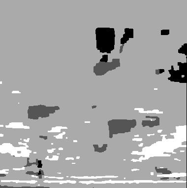
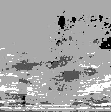
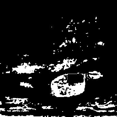
78 Fig. A.1. Case 175T1 (a) Hand Seg. (b) MPM Seg. (c) MPM Diff. (d) ICM Seg. (e) ICM Diff. Fig. A.2. Case 173T1 (a) Hand Seg. (b) MPM Seg. (c) MPM Diff. (d) ICM Seg. (e) ICM Diff. Fig. A.3. Case 101 (a) Hand Seg. (b) MPM Seg. (c) MPM Diff. (d) ICM Seg. (e) ICM Diff.

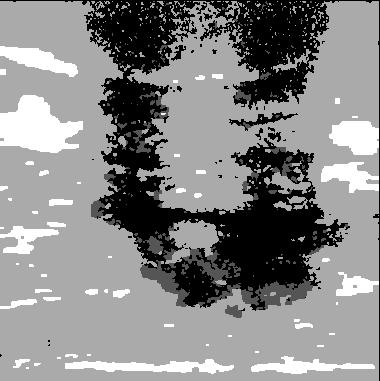
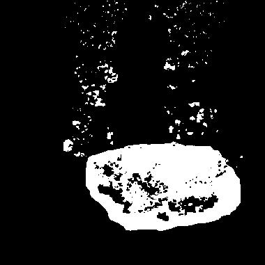
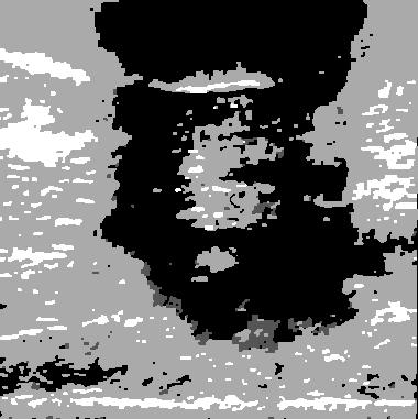
79 Fig. A.4. Case 102 (a) Hand Seg. (b) MPM Seg. (c) MPM Diff. (d) ICM Seg. (e) ICM Diff. Fig. A.5. Case 103 (a) Hand Seg. (b) MPM Seg. (c) MPM Diff. (d) ICM Seg. (e) ICM Diff. Fig. A.6. Case 105 (a) Hand Seg. (b) MPM Seg. (c) MPM Diff. (d) ICM Seg. (e) ICM Diff.

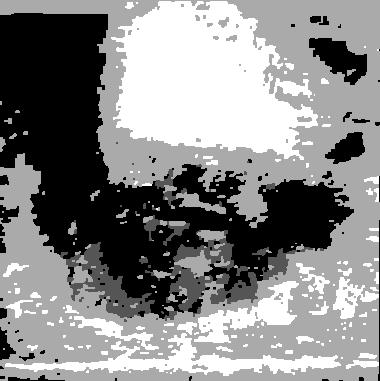
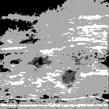
80 Fig. A.7. Case 106 (a) Hand Seg. (b) MPM Seg. (c) MPM Diff. (d) ICM Seg. (e) ICM Diff. Fig. A.8. Case 107 (a) Hand Seg. (b) MPM Seg. (c) MPM Diff. (d) ICM Seg. (e) ICM Diff. Fig. A.9. Case 108 (a) Hand Seg. (b) MPM Seg. (c) MPM Diff. (d) ICM Seg. (e) ICM Diff.

81 Fig. A.10. Case 109, two slices (a) Hand Seg. 45 (b) MPM Seg. - (c) MPM Diff. -(d) ICM Seg. -45 (e) ICM Diff (f) Hand Seg. 50 (g) MPM Seg. - (h) MPM Diff. - (i) ICM Seg. -50 (j) ICM Diff

82 Fig. A.11. Case 117, two slices (a) Hand Seg. 57 (b) MPM Seg. - (c) MPM Diff. -(d) ICM Seg. -57 (e) ICM Diff (f) Hand Seg. 77 (g) MPM Seg. - (h) MPM Diff. - (i) ICM Seg. -77 (j) ICM Diff

83 Fig. A.12. Case 118, two slices (a) Hand Seg. 64 (b) MPM Seg. - (c) MPM Diff. -(d) ICM Seg. -64 (e) ICM Diff (f) Hand Seg. 74 (g) MPM Seg. - (h) MPM Diff. - (i) ICM Seg. -74 (j) ICM Diff Fig. A.13. Case 118b (a) Hand Seg. (b) MPM Seg. (c) MPM Diff. (d) ICM Seg. (e) ICM Diff.

84 Fig. A.14. Case 119, three slices (a) Hand Seg. 16 (b) MPM Seg. - (c) MPM Diff. -(d) ICM Seg. -16 (e) ICM Diff (f) Hand Seg. 65 (g) MPM Seg. - (h) MPM Diff. - (i) ICM Seg. -65 (j) ICM Diff (k) Hand Seg. 74 (l) MPM Seg. -87 (m) MPM Diff. -(n) ICM Seg. -87 (o) ICM Diff Fig. A.15. Case 120 (a) Hand Seg. (b) MPM Seg. (c) MPM Diff. (d) ICM Seg. (e) ICM Diff.

85 Fig. A.16. Case 121, two slices (a) Hand Seg. 12 (b) MPM Seg. - (c) MPM Diff. -(d) ICM Seg. -12 (e) ICM Diff (f) Hand Seg. 43 (g) MPM Seg. - (h) MPM Diff. - (i) ICM Seg. -43 (j) ICM Diff

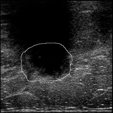
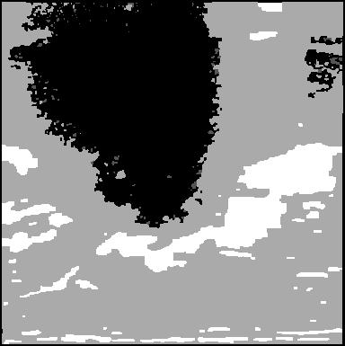
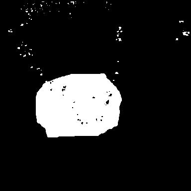
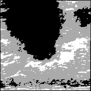
86 Fig. A.17. Case 70 (a) Hand Seg. (b) MPM Seg. (c) MPM Diff. Fig. A.18. Case 78 (a) Hand Seg. (b) MPM Seg. (c) MPM Diff. (d) ICM Seg. (e) ICM Diff. Fig. A.19. Case 81 (a) Hand Seg. (b) MPM Seg. (c) MPM Diff. (d) ICM Seg. (e) ICM Diff.

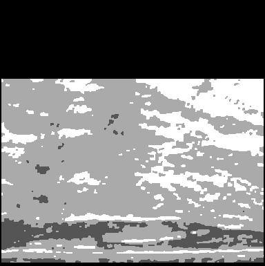
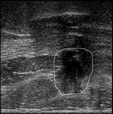
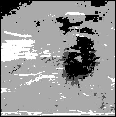
87 Fig. A.20. Case 82 (a) Hand Seg. (b) MPM Seg. (c) MPM Diff. (d) ICM Seg. (e) ICM Diff. Fig. A.21. Case 83 (a) Hand Seg. (b) MPM Seg. (c) MPM Diff. (d) ICM Seg. (e) ICM Diff. Fig. A.22. Case 87 (a) Hand Seg. (b) MPM Seg. (c) MPM Diff. (d) ICM Seg. (e) ICM Diff.

88 Fig. A.23. Case 88, two slices (a) Hand Seg. 47 (b) MPM Seg. - (c) MPM Diff. -(d) ICM Seg. -47 (e) ICM Diff (f) Hand Seg. 72 (g) MPM Seg. - (h) MPM Diff. - (i) ICM Seg. -72 (j) ICM Diff Fig. A.24. Case 89 (a) Hand Seg. (b) MPM Seg. (c) MPM Diff. (d) ICM Seg. (e) ICM Diff.

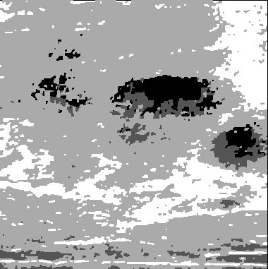
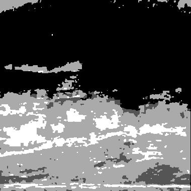
89 Fig. A.25. Case 90 (a) Hand Seg. (b) MPM Seg. (c) MPM Diff. (d) ICM Seg. (e) ICM Diff. Fig. A.26. Case 92 (a) Hand Seg. (b) MPM Seg. (c) MPM Diff. (d) ICM Seg. (e) ICM Diff. Fig. A.27. Case 93 (a) Hand Seg. (b) MPM Seg. (c) MPM Diff. (d) ICM Seg. (e) ICM Diff.

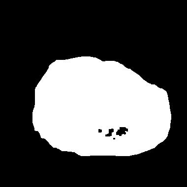
90 Fig. A.28. Case 94 (a) Hand Seg. (b) MPM Seg. (c) MPM Diff. (d) ICM Seg. (e) ICM Diff. Fig. A.29. Case 95 (a) Hand Seg. (b) MPM Seg. (c) MPM Diff.

91 Fig. A.30. Case 95b, two hand segmentations (a) Hand Seg. 1 (b) MPM Seg. (c) MPM Diff. -1 (d) ICM Seg. (e) ICM Diff. -47 (f) Hand Seg. 2 (g) MPM Seg. (h) MPM Diff. -2 (i) ICM Seg. (j) ICM Diff. -2 Fig. A.31. Case 96 (a) Hand Seg. (b) MPM Seg. (c) MPM Diff. (d) ICM Seg. (e) ICM Diff.

92 Fig. A.32. Case 98 (a) Hand Seg. (b) MPM Seg. (c) MPM Diff. (d) ICM Seg. (e) ICM Diff.