c 2007 Salvatore Joseph Candido

Transcription

1 c 2007 Salvatore Joseph Candido

2 MOTION PLANNING FOR BIPEDAL WALKING ROBOTS BY SALVATORE JOSEPH CANDIDO B.S., University of Illinois at Urbana-Champaign, 2005 THESIS Submitted in partial fulfillment of the requirements for the degree of Master of Science in Electrical and Computer Engineering in the Graduate College of the University of Illinois at Urbana-Champaign, 2007 Urbana, Illinois Adviser: Professor Seth Hutchinson

3 ABSTRACT In this thesis I consider the problem of motion planning for walking, bipedal robots, including humanoid robots. While a number of problems complicate planning for robots with a large number of degrees of freedom that possess many dynamic constraints, such as a bipedal system, a simplified framework can be used to find an approximate solution to some planning problems even though, in general, the motion planning problem is intractable. I discuss the difficulties in the motion planning problem for walking robots and summarize previous research addressing the problem. I propose a hierarchical planning framework and outline and discuss two algorithms within that framework. I present results from implementations of these algorithms in simulation environments and discuss the future research required to use this work to create robust and viable motion planning software to deploy on mechanical robotic systems. ii

4 ACKNOWLEDGMENTS I would like to acknowledge and thank my adviser, Professor Seth Hutchinson, for his guidance and sage counsel through every step of my graduate career. I would like to thank Professor Yong-Tae Kim for his collaboration and insight. Finally, I would like to thank my parents for their consistent encouragement and support through this and every other stage of my life. iii

5 TABLE OF CONTENTS LIST OF FIGURES vi 1 INTRODUCTION Path Planning Gait Generation A Combined Approach MODEL Robot Stability Motion Primitives Environment Problem Statement HIERARCHICAL PLANNING Global Plans Subgoal Plans Local Plans GREEDY HIERARCHICAL PLANNER Algorithm Global plan Subgoal plan Local plan Results Discussion DIJKSTRA HIERARCHICAL PLANNER Algorithm Global plan Subgoal plan Local plan Results CONCLUSION Summary Future Work iv

6 A APPENDIX A: SIMULATION ENVIRONMENT A.1 Software Implementation A.2 Robot A.3 Motion Primitives B APPENDIX B: SUPPLEMENTAL GHP RESULTS B.1 Map B.2 Map 2, Course B.3 Map 2, Course B.4 Map 2, Course B.5 Map 2, Course B.6 Map REFERENCES v

7 LIST OF FIGURES 1.1 Humanoid robots Passive walking robots Stable versus unstable locations for the ZMP-COP Comparison of different V s for a polygon in the plane Workspace, navigation map, and terrain discontinuity map for an example environment Workspace, skeleton of M nav, and global path overlayed on M d for an example environment Simulation results in workspace Simulation results in workspace Simulation results in workspace Global plan does not consider the number of subgoals Global plan gives maximum clearance on M nav but not M d (pictured) GHP failure on workspace Algorithm flow charts Maps used by the DHP on workspace 3 and the path through the graph Simulation results for DHP in workspace Maps used by the DHP on workspace 2 and the path through the graph Simulation results for DHP in workspace B.1 Maps for workspace B.2 Path for workspace B.3 Maps for workspace 2, course B.4 Path for workspace 2, course B.5 Maps for workspace 2, course B.6 Path for workspace 2, course B.7 Maps for workspace 2, course B.8 Path for workspace 2, course B.9 Maps for workspace 2, course B.10 Path for workspace 2, course B.11 Maps for workspace B.12 Path for workspace vi

8 1 INTRODUCTION Humanoid and other legged robots present an exciting new challenge to the discipline of robotics. Although robots such as Honda s Asimo [1], Kawada s HRP-2 Humanoid Robot [2] and Sony s QRIO [3] (Figure 1.1) are not yet widespread, the potential impact of anthropomorphic robots is enormous and requires study. While there are many clever robot designs that are successful for their respective tasks, no existing robot comes close to approaching the utility of a human across a wide range of tasks. The potential commercial and societal impact of humanoid robotics are large. Humanoids could fill voids in the labor market where workers cannot be attracted at a sufficient rate. As an example, scientists are working to develop robots to care for elderly and handicapped patients (e.g., [4, 5]). Also, humanoids could perform tasks that are dangerous for humans to perform. Research has been done on robots that will perform dangerous work on construction sites (e.g., [6]). Remotely operated humanoid robots could (a) Honda Asimo (b) Sony QRIO (c) Kawada s HRP-2 Figure 1.1: Humanoid robots 1

9 fight fires, disarm bombs, perform repairs in radioactive areas and assist the military in circumstances that, for a human, entail significant risk or loss of life. Research has been done to develop controllers for teleoperation of humanoid robots (e.g., [7]) that could be used in these hazardous environments. Humanoid robots conceivably have the potential to perform any task mundane or dangerous for humans. As we continuously demand a greater number and wider range of tasks to be automated, it seems as though there is a place for a general purpose, autonomous robot. However, why should we believe that an anthropomorphic robot is a good or the best blueprint by which to engineer a robot to fill this need? Although our narcissism may be partially driving our creation of the humanoid as the ultimate robot, a few simple reasons can be given to demonstrate the pragmatism of the humanoid. First, it may be easier for humans to adjust to and accept autonomous humanoid robots (and those mimicking other domesticated animals) because of the familiarity we have with those morphologies [8]. Second, the environments we have crafted for thousands of years are designed for human interaction and use. In order for a robot to fully take advantage of these environments, it should be able to mimic the actions and behaviors of humans. While the motivations of engineering legged robots are clear, two related but distinct problems complicate the design of control of movement for these robots. Analytical and computational problems are presented by both the robot s complex geometry and its nonlinear system dynamics. The first problem is typically addressed by the robotics path planning community. The control systems and computer science communities address the second problem using a variety of means. Both problems must be addressed and solved 2

10 in an interoperable manner in order to create humanoid robots capable of functioning in environments built and populated by humans. In the following two sections, I will discuss the difficulties of the two primary problems of walking robotics and summarize the work that has been done to address these difficulties. I will then discuss an approach using motion primitives that combines the work done on both problems. I will summarize the prior work done using motion primitives with walking robots. Finally, I discuss my approach within the motion primitives framework and outline the remainder of my thesis. 1.1 Path Planning The field of path planning is concerned with algorithms to automate the movement of robots, parts, or other geometric objects through arbitrary environments. The prototypical task is to move a robot in its workspace (environment) from one position and orientation to another desired position and orientation without the robot colliding with obstacles. Whether studying robots modeled as points on a plane, surface meshes comprised of millions of triangles, or pianos, motion planning has applications within and outside of robotics. Character animation, manufacturing, pharmaceutical design, exploration and mapping of unknown environments and high-level control of autonomous vehicles are just some of the problems impacted by the field of path planning. The most basic navigation problem is to move a robot modeled as a point in space through a two-dimensional environment with various forbidden (or obstacle) regions that the robot may not enter. The model is kinematic, meaning the only restriction is that the robot must move along a continuous path. This problem has been exhaustively studied and many solutions ex- 3

11 ist. Bug algorithms [9], navigation functions [10], cellular decompositions [11], and roadmaps such as the visibility graph [12,13] and Voronoi diagram [13,14] present complete algorithms that will guide the robot to its destination. These methods have been extended to robots of arbitrary shape. The most important distinction is that the robot is modeled as a point in an abstract configuration space rather than in the workspace. A configuration is a specification of every point on the robot and the configuration space is the set of all feasible configurations [13]. Essentially, planning is complicated by the fact that the robot s orientation and internal joint angles can be changed in addition to just the robot s position. A robot at one orientation may fit through a space where the robot would collide with an obstacle if it were at a different orientation. This adds additional dimensions of possibilities for a path planning algorithm to check, and presents a much higher level of complexity. Simple robots, such as point robots (or cylindrical robots) with orientation, rods, and polygonal robots, can make use of the aforementioned algorithms by various extensions and the computation of the Minkowski sums [15] of the robot with the workspace obstacles. The classic example of path planning is the piano mover s problem [16]: moving a piano through a house in such a way that the piano does not collide with other objects in the house (or the house itself). Only the geometry of the objects and not the forces acting on the piano, such as gravity, is considered. Extending the analogy, the piano would be assumed to have infinitely strong and infinitesimally small movers. Thus, the piano mover s problem is only concerned with moving a geometric shape along a trajectory that is continuous in space through an environment. Complete algorithms that are tractable exist only for special cases of the path planning problem. In the general case, Schwartz and Sharir [11] have 4

12 given an algorithm that has a doubly exponential time complexity with respect to the degrees of freedom of the robot. Canny [17] gave an improved algorithm that is singly exponential in time and showed the motion planning problem is PSPACE-complete. Even simplified problems such as finding threedimensional shortest paths in the presence of obstacles is NP-Hard [17]. This means the problem is solvable, but no algorithm is known to solve it in an amount of time that is a polynomial function of the input [18]. This means that as the problems become harder, it is believed that in practice we cannot solve them in an acceptable amount of time, regardless of the growth in computational power. Canny s algorithm in the general case is the best known complete solution to the general path planning problem. No known complete algorithm for this problem has a faster worst-case running time, so it provides an upper bound on the number of operations required to solve an instance of a path planning problem. The running time of Canny s algorithm is p m log p w O(m2 ) where p is the number of polynomials required to represent the robot s configuration space, w is the highest degree of any of those polynomials and m is the number of degrees of freedom of the robot. In addition to the dependence on the number of degrees of freedom of the robot, there is also a nonlinear dependence on the size of the environment. A typical bipedal robot has around 12 degrees of freedom in its legs, and a humanoid robot will typically have 28 or more degrees of freedom. This large number of actuators arranged in a bipedal form creates high dimensional, extremely complex configuration and state spaces. Additionally, humanoid robots are expected to function in large, 5

13 complex environments. In practice, this problem is well beyond the domain of classical path planning algorithms. Due to the underlying complexity of the path planning problem, as the configuration spaces grow, probabilistic, sample-based methods and other approximation or heuristic methods are more commonly used. The Probabilistic Roadmap (PRM) method [19] uses random sampling of the configuration space as a preprocessing step to build a roadmap in that configuration space. This creates a data structure that can be repeatedly queried to produce paths between arbitrary start and goal configurations. The Rapidly-exploring Random Tree (RRT) [20] expands throughout the robot s configuration space to find paths to the robot s desired destination. These algorithms have been shown to be probabilistically complete. Probabilistically complete algorithms satisfy the following criterion lim p f(k) = 0 (1.1) k where p f is the probability of failure given k samples when a solution exists. This means that as the number of samples goes to infinity, if a solution exists the probability of finding it goes to 1. RRT s have the additional advantage that they extend well to robots with nonholonomic constraints. Classical robot path planning algorithms ignore the constraint that a car may only move forwards and backwards and may not slide sideways into a narrow parking space along the side of a street. These classical algorithms would not return feasible plans in some cases and additional machinery would need to be added to generate a plan to parallel park a car. By forcing each iterative expansion of the RRT to obey the constraints of the system model, RRT s can plan feasible motions for cars, airplanes, differential drive robots, and a variety of other systems. 6

14 While sample-based methods are powerful tools, planning for walking robots has requirements that sample-based methods are not designed to meet. Walking robots have small ranges of stable gait trajectories. While their configuration spaces have high dimension, many configurations will cause the robot to fall over or damage itself. Sample-based methods, in contrast, are designed to be expansive in their search of the configuration space to make the guarantee of probabilistic completeness. Also, it is difficult to use these methods while attempting to optimize for one or a combination of criteria. Some criteria that may be desirable are minimizing energy consumed, minimizing time to reach a destination, and maximizing stability and robustness, which is equivalent to minimizing the chance of an accident. The expansive nature of sample-based methods precludes using a control that is optimal at every given point in the search. For example, if a sample-based algorithm that selects its samples randomly is run twice it will likely produce two different motions due to the random nature of the algorithm. If there is a cost criterion, most likely one of these motions will be superior to the other. In the case of a walking motion, it would be desirable to use the better motion repeatedly. This seems to imply that using a random sample-based method to plan each step would be computationally inefficient as well as costing the system more to implement the plan generated. Deterministic sampling schemes, while always generating the same motion for a given set of inputs, also do not, in general, produce optimal trajectories. Finally, perhaps the most difficult constraint is related to the aesthetics of movement. It may be desirable for the robot s motions to mimic human motion. For these reasons, sample-based methods, when relied upon solely, do not appear to be the solution for humanoid motion planning. 7

15 1.2 Gait Generation Due to the complexity of the path planning problem, researchers and engineers often concentrate on generating short movements, such as a single step, or repeating gaits in an environment free of obstacles. This problem of gait generation is the second core difficulty of motion planning for walking robots. Leaving aside the geometric aspects discussed in the previous section, the mechanical systems of a walking robot are not easily controlled. A walking robot has nonlinear system dynamics. This system of equations will have only a small range of trajectories that keep the robot from falling, a stability requirement, and the control inputs to the system will be bounded as the motors can only exert a torque up to some maximum amount. This mathematical model is generally difficult to analyze and may not even have an explicit, closed form solution. Even ignoring the geometry of the environment, gait generation methods must take into consideration collisions between links of the robot (self-collisions). Also, additional modeling difficulties come into play. The contact between the supporting foot of the robot and the ground is not a perfect joint. The support foot may slip at times when it should not move, and friction may make moving a support foot difficult. Also, the model must consider the impact force applied when the robot s foot first contacts the ground and frictional forces in the joint. Models must be carefully developed and experimentation is required when building mechanical systems. This problem of gait generation is not a straightforward one. A number of approaches are commonly taken. One approach is to develop a gait and design a controller to track a pattern of joint movements. Gaits are generated manually in some cases by a human designer s intuition or by using motion capture to directly mimic human motion [21]. Computer algorithms such as 8

16 neural networks, fuzzy logic, learning, and genetic algorithms can also be used to find gait trajectories for the robot [22,23]. While these methods rely heavily on carefully following a preset trajectory, a second approach relies heavily on feedback to stabilize the robot. Control policies based on the robot s zero moment point [24, 25] are common examples of this methodology. By looking at and controlling indicators of system behavior such as the center of mass, center of pressure, or zero moment point, controls are designed that produce (typically) statically stable gaits. Other interesting methods based on the tools of nonlinear control are virtual model control [26] and hybrid zero dynamics [27]. Both methods use artificial constraints enforced by controllers to simplify the system model to aid the production of a gait. While not being required to track a specific trajectory, these feedback methods, particularly zero moment point control, are largely energy inefficient. Energetic cost of transport (COT) is a measure of the efficiency of a mechanical system s conversion of energy to locomotion. Essentially, it is the amount of energy consumed divided by the weight and distance traveled [28]. For example, Honda s Asimo, which uses zero moment point control, has a COT of 3.2 that is approximately ten times the COT of a walking human (e.g., [29]). Efforts to make walking bipeds more energy efficient have found inspiration from passive walking devices. These are mechanical devices that walk down an incline without using motors or batteries. Given some initial kinetic energy, these passive walkers rely only on conservation of momentum and the potential energy released by moving down the incline to keep them in motion. They were first analyzed in [30]. An energy-efficient approach to biped locomotion derived from this work combines the principles of passive walking together with controlled feedback [31]. In [31], a nonlinear control is used that replicates the 9

17 (a) McGeer s planar walker [30] (b) 3D walker built by Collins et al. [33] (c) Collins walker with active control based on passivity principles [32] Figure 1.2: Passive walking robots principle of passive walking down an incline on arbitrary ground slope. These methods have been shown to be more efficient than strict trajectory tracking methods and it has been conjectured that this approach models the behavior of humans and animals (e.g., [32]). Some robots based on the principles of passive walking are shown in Figure 1.2. While progress has been made, it appears that the problem of gait generation will be difficult to extend to plan paths in the presence of obstacles or in complex environments. So far, gait generation methods have been demonstrated only in environments free of obstacles with flat or slowly-varying surfaces and environments with simple, repeating geometry, such as stairs. It is my conjecture that a fusion of both gait generation and path planning is useful for bipedal motion planning. Both path planning and gait generation methods have drawbacks. However, when combined in a coordinated manner they can amplify one another s successes while partially attenuating the other s deficiencies. 10

18 1.3 A Combined Approach As both the path planning and control problems are known to be difficult both analytically and computationally, some approaches to navigation for humanoid robots are based on a simplification of the humanoid motion planning model. One strategy that combines the benefits of both the gait generation and path planning approaches is the use of motion primitives. Motion primitives are control policies that when activated from a specific initial configuration take the system to a specific final configuration in a set amount of time. Essentially, they are patterns of motion that can be used in sequence to convert one or more preplanned steps into a path for the robot. Some approaches that use motion primitives for humanoid motion planning are described in [34,35]. While a motion primitive is actually composed of a complicated series of motions, motion planning algorithms can represent a motion primitive with only a few parameters. Also, the robot s controller needs only to store the controls necessary to execute the motion primitive. An algorithm can then sequence together motion primitives to form a path through the workspace and then pass the sequence to the robot s controller to execute the movements. By describing the movements of the robot as a set of motion primitives and using a set of heuristics to validate footstep locations, it has been demonstrated that planners can find paths through some cluttered environments [34]. Motion primitives can take the result of a gait generation method and then use it in a framework that can take into account obstacles and terrain, so long as the different gaits guarantee the robot will not fall and that the robot can switch between different gaits. Path planning for a humanoid robot on flat ground can be considered as a search for a sequence of feasible motion primitives rather than a search of 11

19 a high dimensional configuration space for a trajectory [34]. A search algorithm can, in many cases, quickly find a sequence of motions to take the robot to its destination. However, a search will require exponentially more checks as the number of motion primitives in that path increases. In environments with obstacles, stairs, inclines, and holes, the motions of humanoids are constrained by more than just placements of the robot on the plane. A large set of motion primitives is required to traverse these environments. An A* search or forward dynamic programming algorithm may take considerable time to compute a sequence of motion primitives or the problem may become computationally intractable. Some hierarchical planning approaches have been applied to control the growth of complexity and find an approximate solution to this problem [36 38]. My interest is to explore the design of hierarchical motion planning algorithms for bipedal, walking robots. Hierarchical algorithms build heuristics that allow a robot to use motion primitives in order to efficiently navigate complex workspaces. Using a finite number of motion primitives that move the robot by discrete intervals, this problem will always be one of search. However, the hierarchical methods place heuristics on that search, making an intractable search problem into one that can be approximated by an implementable, efficient algorithm. As with all heuristic methods, there is a trade of efficiency for completeness but the simulations presented in this thesis demonstrate that, in practice, the trade is acceptable in most cases. In this thesis, I propose two path-planning algorithms for bipedal robots. The first algorithm is the Greedy Hierarchical Planner (GHP), which finds a path between the robot s initial configuration and a set of goal configurations. I show simulation results for this algorithm using a simulated humanoid robot in simulated environments. The second algorithm is a refinement of the GHP 12

20 called the Dijkstra Hierarchical Planner (DHP). The DHP eliminates some of problems present in the first algorithm. I also show simulation results for this algorithm including on inputs where the GHP has failed or gives an undesirable result. This thesis proceeds as follows. In Chapter 2, I introduce the mathematical model being used and the assumptions being made throughout this thesis. Once the model is established, I then formally define the problem I am solving. In Chapter 3, I describe the conceptual framework being used to solve the problem. In Chapters 4 and 5, I present the GPH and DHP, two algorithmic realizations of this framework, and show simulation results. Finally, in Chapter 6, I discuss my results and some future directions for this research. 13

21 2 MODEL In this chapter I define the models that will be used throughout this thesis. I discuss the model of the robot, its environment, the movements of the robot, and the motion planner s interactions with all of these. I note the assumptions implicit in the model and then use this construction to precisely define the problem that I solve. 2.1 Robot The robot s shape s is an ordered list of all the joint positions of the internal degrees of freedom of the robot. The robot is assumed to be a collection of rigid links whose positions and orientations, relative to one another, are defined by the positions of the joints linking them together. The set A i denotes the set of points in the world occupied by the i th link. A configuration of the humanoid (or bipedal) robot is a complete specification of every point on the robot [13]. The location of a coordinate frame rigidly attached to the robot in an arbitrary but defined place is denoted by x SE(3). This coordinate frame specifies a transformation between a fixed world coordinate frame and a specific link of the robot. A configuration can then be parametrized with the following representation: q = (x,s) (2.1) 14

22 A configuration, q Q, encapsulates the shape of the robot and its position and orientation in the workspace. The notation Q refers to the configuration space, which is the set of all possible configurations. A parametrization of the configuration, when combined with a specification of the geometry of each link A i can be used to uniquely determine the coordinates of every point on the robot. This is done by utilizing a set of forward kinematic equations. The robot s state is the information necessary to characterize the dynamics of the robot. It consists of the robot s configuration and the first time derivative of the configuration. The derivative is specified by scalar values for position and each internal degree of freedom and a matrix belonging to the Lie Algebra of 3 3 skew symmetric matrices of SO(3) [39]. The union of A i s over all the robot s links gives A, the set of points in the world occupied by the robot. Typically, A is modeled in computer simulation as a set of triangles that when seamed together constitute an approximation to the boundary between points belonging to and outside of A. This is referred to as a mesh. This mesh can be displayed as a solid structure or used for collision detection with another mesh representing obstacle boundaries in the environment. Commonly, the configuration space of a bipedal robot is Q = SE(3) T m where T m is the m-dimensional torus. This refers to a robot with m revolute and no prismatic joints. This could corrospond to a robot built from m servo motors. In some bipedal locomotion literature, a configuration space of SO(3) T m is used. This is because obstacle-free environments are considered and the location of the robot with respect to a fixed world frame is not important. The robot s configuration is specified relative to one of the robot s links. In my work, it is essential to know not only the robot s shape and orientation 15

23 with respect to the gravity vector but also the robot s position with respect to the environment. A typical bipedal robot will have two legs and some form of a weighted torso. Often, links that act as ankles and feet will be included in the design to facilitate smooth, efficient walking. Actuators are placed at the knees, hips and ankles, although some underactuated systems exist that omit some or all of these motors (e.g., [40]). For robots typically classified as humanoid, the torso is attached to links that correspond to two arms and a head. Humanoids typically have at least 28 degrees of freedom, 12 of which are below the robot s waist. In the gait generation literature, the frame specifying the robot s position and orientation with respect to the environment x is often attached to the foot of the robot contacting the ground. Throughout my thesis, I will refer to this as the support foot. As the support foot changes with every step, planning and control occurs on a hybrid system whose switching events occur when either one of the robot s feet make or break contact with a support surface. When only one foot is in contact with the ground the mode of support is said to be single support. When both feet contact the ground the mode of support is said to be double support. In the humanoid motion planning and character animation literature, it more common for x to be attached to the robot s torso. It is often referred to as the root frame or the body-attached frame. Under this convention, while still a hybrid system depending on the current mode of support, only the equations of motion change as the support mode changes. The configuration varies continuously as opposed to the case when the body-attached frame jumps between feet when the support mode changes. I will adopt this latter convention in my thesis. 16

24 2.1.1 Stability With many types of robots (e.g., wheeled mobile robots), almost every configuration that does not cause a collision with the environment is a suitable placement of the robot. This is not necessarily the case with walking robots. With a walking robot, the primary issue is to avoid the robot falling. More interesting problems cannot be addressed without satisfying this basic objective. Unfortunately, there will be many configurations that do not induce a collision and are within the robot s joint limits that will not allow the robot to stand upright. When discussing stability for a walking robot, it is important to distinguish between postural stability and gait stability [41]. Postural stability refers to the ability of the robot to remain unmoving at a specific configuration. It is important to consider both the robot s location in the environment x and its internal shape s. Regardless of the location of the robot in the world, and so long as the support surface is at the same orientation, certain shapes of the robot will stand upright and others will fall. Gait stability, on the other hand, is associated with a controller moving the robot on a nominal trajectory in the shape space. Measures of gait stability correspond to measuring how well the controller is able to attenuate perturbations that push the state away from the nominal trajectory [41]. Postural stability deals with the robot s ability to maintain an unmoving configuration while gait stability deals with the robot s ability to maintain an unchanging gait motion. A natural way to characterize postural stability of a bipedal robot is to differentiate the states in which a robot can apply a control to stay upright from the states that will definitely cause the robot to fall. This has been discussed in [42] and is termed a viability condition. Let F Q be defined 17

25 as the set of configurations where the robot is considered to have fallen. For example, configurations where a link other than the robot s feet is in collision with the ground would be one way to choose F. Then, a state at time t 0 is considered viable if and only if there is a control that can be applied at that state so that the state at time t is not in F for all t t 0. Keeping the robot in the viable region of the state space is a necessary condition for motion planning. While an explicit characterization of states as viable or not would be extremely useful, in practice it is difficult to compute. One could attempt to approximate the set of viable states by finding equilibrium points and cyclic trajectories and then computing trajectories from various states to them. However, considering the dimension of the state space and the complexity of the system dynamics, the problem is computationally intractable. Instead, it is much more practical to look for subsets of the set of viable states that can be easily checked. One way to check if a robot can maintain its stance is by looking at the location of the robot s zero moment point (ZMP) or center of pressure (COP). The ZMP of the robot is related to inertial and gravitational forces while the center of pressure is related to the contact forces of the robot. The two points are necessarily coincident [43] and can be referred to as the ZMP-COP. With an elementary knowledge of static mechanics, it is known that every system of forces and moments can be replaced by an equipollent 1 resultant force system of a single force and moment acting on a specific point. The simplest resultant of a general system is one that reduces to a single force with a parallel moment [44]. The center of pressure is the point on the ground where the equipollent resultant force system of the contact forces on the robot s feet has zero tipping moment, the tipping moment being 1 Two different systems of forces are said to be equipollent if they make the same contributions to the equations of equilibrium; the sum of the forces and sum of the moments are both equal to zero in a static system [44]. 18

26 (a) Single support (b) Dual support Figure 2.1: Stable versus unstable locations for the ZMP-COP the component of the moment tangential to the supporting surface. The ZMP is defined as the same with respect to the equipollent resultant force system of the inertial and gravitational forces on the robot. If this ZMP-COP point is strictly within the region of support, the robot will not fall over. If the robot has both feet on the ground it is in dual support and the region of support is the area within the convex hull of the robot s feet. If only one foot is on the ground then it is in single support and the region of support is simply the area covered by that foot (see Figure 2.1). If the point leaves this area the forces acting on the robot will cause the robot to rotate around the ZMP-COP and the robot will tip and fall. For a detailed discussion of this subject see [42,43]. A walking robot is said to be in an equilibrium state when the following criteria are satisfied: 1. The moment (torque) around the robot s ZMP-COP is within the region of support for the robot. 2. The torque or force incident on every joint is less than or equal to the maximum torque or force that the robot s actuators can apply to that joint. 3. Every joint of the robot is within its feasible range. 4. The robot is contacting a support surface with at least one of its feet. 19

27 5. The robot s links are not in collision with one another. (An equivalent condition that the volume of A is the same as the sum of the volumes of A i for all i.) 6. The robot s links, excluding the foot contacts with the support surface, are not in collision with any surfaces or obstacles in the workspace. This ensures that the robot is in the free configuration space (Conditions 5-6) and can maintain its configuration indefinitely, so long as its actuators remain powered and it is not perturbed (Conditions 1-4). The second stability notion for a walking robot is gait stability. There are a number of methods of characterizing whether a controlled gait trajectory rejects disturbances and attenuates perturbations. A gait that is comprised of only equilibrium states is said to be statically stable [41]. In many cases this is a useful criterion, as the robot can stop at any time and will not fall over. Honda s Asimo relies heavily on zero moment point control to generate gaits, and all of its motions are statically stable [1]. While this may seem ideal for safety purposes, statically stable gaits are typically not energy efficient. Many gaits that are not statically stable are used for bipedal robots, largely in the research area of passive walking. In order for one of these gaits to be useful, the state trajectory of the robot must fall into a limit cycle so the same motion can be repeated, or it must reach an equilibrium position so the robot can stop. A gait that requires the ZMP- COP to leave the convex hull of the robot s region of support but is able to regulate the trajectory to a nominal trajectory in the presence of disturbances is referred to as dynamically stable [41]. In this thesis, I will not be concerned with the specifics of postural or gait stability. The main idea of this thesis revolves around motion planning with 20

28 a given set of gaits. It will be required only that the gaits encapsulated in the set of motion primitives exhibit dynamic stability with a sufficiently large basin of attraction to handle common disturbances and the final configuration of the robot is in an equilibrium state. However, it is important to keep these stability notions in mind when designing gaits and choosing a set of motion primitives. 2.2 Motion Primitives A motion primitive is a control policy that when activated at time t from a configuration with a specific initial shape, s(t) = s i, takes the system to a configuration with a corresponding specific final shape, s(t + τ) = s f, after τ seconds have elapsed. Essentially, a motion primitive encodes a repeatable pattern of motion that the robot can perform any time its shape is s i. For example a motion primitive might be the motion associated with a single step. The generation and use of motion primitives has been demonstrated in [25, 34, 35]. The planning algorithm requires only specific parameters of each motion primitive to compute the sequence of motion primitives to be used to navigate the environment. Thus, each primitive is parametrized by the following set: P = (x,s i,s f, c, τ,v) (2.2) The net displacement of the robot s root frame in SE(3) during execution of the motion primitive is x. The initial and final shapes the robot will take while executing the motion primitive are s i and s f. The cost of executing this primitive is c. The amount of time the robot takes to execute the motion primitive is τ. A bounding volume V contains the swept volume the robot moves through while executing this motion primitive. The cost typically encapsu- 21

29 lates a combination of time, energy, risk (potential instability), and general desirability of a given motion. The swept volume is the union of the set of all points on the robot at every instant of time during execution of the primitive. The bounding volume V is either the swept volume or a superset of the swept volume, and is used for fast collision checking. As the motion primitive produces a repeatable motion, the bounding volume can be precomputed and stored by the path planning algorithm. By placing the bounding volume at the location of the robot in the workspace, the path planning algorithm can quickly check for collisions with workspace obstacles without calculating any motions of the robot or recomputing the location of the robot s links while executing those motions. In practice, V could be the swept volume [45], an approximate bounding volume [46], a bounding box, or an axis-aligned bounding box. Each one of these has trade-offs between computational expense and precision of the approximation. A swept volume is difficult to construct and testing for collisions against polygonal meshes may require a lot of computational operations, but the collision checking is exact. In contrast, an axis-aligned bounding box is simple to construct and testing for collisions is trivial. However, in many cases, too many potential collisions are reported where the robot would actually be far from any obstacle because the bounding volume is an overly conservative approximation. Requiring V only to bound the swept volume, in practice, allows an approximation that is arbitrarily close to the actual swept volume, although a high degree of precision is often unnecessary. Figure 2.2 shows a planar example comparing these three options for choosing V. Use of motion primitives can be thought of as restricting the trajectories allowed in a continuous planning problem to turn it into a discrete problem 22

30 (a) Swept volume of polygon (b) Bounding volume containing the swept volume (c) Axis-aligned bounding box Figure 2.2: Comparison of different V s for a polygon in the plane with a finite action set. This defines a discrete transition function q f = f(q i, P) (2.3) where q f = (x f,s f ), q i = (x i,s i ) and x f = x i x where x SE(3) is a constant transformation that is a parameter of P. A sequence of motion primitives is denoted as γ = (P 1, P 2, P K ). By iteratively expressing the configuration using Equation (2.3) as each P i is applied after P i 1, the final configuration after applying the motion primitives of γ at q i can be found. Thus, the transition function can also be defined for sequences of motion primitives q f = f(q i, γ) (2.4) where x f = x i x 1 x 2 x K and x k is the x parameter of P k. The ideal set of motion primitives is one that allows the robot to move between any two configurations in the environment if a path that the robot could follow exists. Pragmatically, such a set of motion primitives is not available. As more motion primitives are provided to the robot, more paths through the environment can be found. Typically, the robot is supplied with motion primitives for walking and turning gaits. It should have primitives for stepping onto ledges and walking on inclines (if such behavior is desired). 23

31 Motion primitives that are small steps are useful for adjusting the location and orientation of the robot by small amounts. A motion primitive can be thought of as specifying a sequence of internal shape changes while its parametrization describes the motion of the robot in its ambient space. The configuration of the robot is changed through the application of motion primitives that are chosen by the planner. A motion primitive P when applied to the current configuration q produces a new configuration q. The robot s controller takes a motion primitive and executes the underlying motion on the robot. The system can then be thought of as a discrete model where at every stage a new motion primitive is applied to move the robot to a new configuration time τ later (where τ depends on the motion primitive chosen). In order to sequence motion primitives together to generate a composite motion, there must be some guarantees that the robot will be able to move along subsequent motion primitives. First, the final shape of one motion primitive must match the initial shape of the next motion primitive. Second, the robot must be able to switch between the two primitives in the state trajectory. One way to guarantee this is to require initial and final positions to be equilibrium positions for the robot (statically stable). However, this is only a sufficient condition. What is required is a guarantee that the robot can switch between subsequent motion primitives and the final motion primitive ends in an equilibrium for the robot. Given a set of motion primitives, the relationships encoding which motion primitives can transition to other motion primitives can be stored using a finite state machine that can be quickly accessed by a motion planning algorithm. There is a great deal of flexibility when choosing a set of motion primitives for the robot, but some factors are important to consider. The designer should 24

32 ensure that s f for every motion primitive matches an s i for at least one other motion primitive. Otherwise, some motion primitives could become terminal motions. Also, a set of motion primitives should be chosen so that the robot can always adjust its position by small amounts in all directions. This is important so the robot will not become stuck in certain configurations in the environment. Finally, motion primitives should be included in order to traverse all the geometry, such as stairs or ramps, the robot will encounter in the environment. This does not require complete knowledge of the environment in advance but instead only key information like the height of steps or the pitch of ramps. The details of the set of motion primitives I have chosen for the simulations shown in this thesis are given in Appendix A. 2.3 Environment A walking or humanoid robot operates in a workspace that is a subset of R 3. The floor is assumed to be mostly on a plane perpendicular to the gravity vector. Obstacles, ramps and holes in the floor may be sparsely scattered throughout the environment. Obstacles are assumed to have steep side walls. Basically, these assumptions correspond to typical indoor environments. The motion planning algorithm is assumed to have a three-dimensional polygonal map of the robot s workspace denoted as W R 3. Often, this will be stored as a triangle mesh of the environment for collision checking against a simulation model of the robot. It is assumed that information about the height of the floor (or obstacles sitting on the floor), height of the ceiling, and orientation of the floor can be easily extracted from this map. 25

33 2.4 Problem Statement The task of the motion planning algorithm is to find a sequence of motion primitives that, when applied, move the robot from a given initial configuration, q init, to a configuration in a desired goal region, Q goal Q. The set Q goal will correspond to the robot s body-attached frame being in some region in the workspace, B goal SE(3), and the robot being able to maintain that position. Thus, every q = (x,s) Q goal will have the properties that x B goal and s is at an equilibrium. Given q init, B goal, the model of the robot A, a set of motion primitives P, and a model of the environment W, the goal of the motion planner is to find a sequence of motion primitives γ that satisfies the following conditions: 1. f(q init, γ) Q goal. 2. The bounding volume V of P k is not in collision with any obstacles when placed at f(q init, γ). 3. For all P k in γ, s i of P k is the same as s f of P k 1 and s 1 = s init. 4. The foot contact orientation of s i and s f of P k match the support surface at q i and f(q i, P k ), respectively. Furthermore, the planner should seek to minimize the cost of the path, the sum of the costs of each primitive in the sequence. In the next chapter, I will discuss the general framework of the hierarchical planning algorithms I propose in this thesis that find paths that satisfy the problem statement given in this section. 26

34 3 HIERARCHICAL PLANNING This chapter describes the conceptual framework used by the specific planning algorithms proposed in the following chapters. I will describe the problems of planning with only a set of motion primitives and propose the outline of a solution. In Chapters 4 and 5, I describe two realizations of this framework in algorithmic form and the results of simulation implementations. A significant portion of the complexity of planning for walking robots comes from finding motions in a configure space with a large number of dimensions. The primary benefit of motion primitives is that the trajectories of the robot s internal degrees of freedom have already been planned in advance, possibly at great computational expense. Each motion primitive is parametrized, as in Equation 2.2, and planning can occur using a finite set of discrete actions in SE(3). This is a large computational savings over planning in the original configuration space of the robot. Furthermore, since the joint trajectories are computed in advance of planning and reused, more time and effort can be applied to ensure the quality of the motions. Essentially, instead of planning in the continuous configuration space with many dimensions, the problem becomes a search through sequences of motion primitives that move the bodyattached frame of the robot in a six-dimensional space. Care must be taken to ensure the robot will not collide with obstacles or reach an unstable position, but this can be largely decoupled from the planning problem. Although a pure search algorithm may work for short sequences, in general the problem is an intractable one and requires exponentially more operations each time the length of the sequence of motion primitives increments. Further- 27

35 more, as the number of available motion primitives increases, the branching factor of the search increases as well. One method to compute sequences of motion primitives in a feasible amount of time is to use a hierarchical planning algorithm. Hierarchical planning refers to planning occurring at different levels of precision by a series of component algorithms. Each algorithm takes the work of previous components and refines it until, at the lowest level, a sequence of motion primitives is specified. In this thesis, I propose hierarchical algorithms consisting of a global plan, subgoal (or waypoint) plan, and local plans. A decomposition of the three-dimensional workspace is encoded into a set of two-dimensional maps. The global planner builds a navigation map from knowledge of the environment and returns a path through the free space of this navigation map. The subgoal planner chooses appropriate cuts on this path between which to find local plans. The local planner transforms these segments of the global path into sequences of motion primitives that the robot can use to move from start to goal positions in the workspace. Essentially, the higher level layers of the algorithm build heuristics that guide a series of traditional searches that are small enough to compute quickly. I will now describe the components of these hierarchical algorithms. 3.1 Global Plans The task of the global planner is to find a candidate route through a twodimensional, simplified representation of the workspace between the point corresponding to q init and the area of the map corresponding to B goal. In order to do this, the planner makes assumptions that greatly simplify the model of the robot and environment, and creates a rough sketch of the path the robot will traverse. 28

36 Although planning with motion primitives is a discrete planning problem that occurs in SE(3), many points in SE(3) will (hopefully) never be reached. In almost all desired cases, the robot will remain upright, the body-attached frame will be translated within a range of distances from the ground and the body-attached frame will have approximately the same orientation except for rotation around the axis pointing up through the robot s body. Assuming the robot is at the correct height and orientation for all the support surfaces in the world, an approximation can be made and this level of planning can occur in SE(2). Therefore, the workspace will be compressed to a two-dimensional map containing free and obstacle regions and the robot will be modeled as a bounding area with position and orientation. Because the robot is assumed to have a variety of motion primitives allowing a large range of movements, we assume that motion primitives can be selected to move the robot s projected area a small amount in any direction. As discussed in Chapter 2, the motion planner is assumed to have a threedimensional polygonal map of the robot s workspace and information about the height of the floor (or obstacles sitting on the floor), height of the ceiling and orientation of the floor can be easily extracted from this map. Using this data the motion planner constructs a two-dimensional map to be used by the global planner, storing a binary value for each (x, y) R 2 corresponding to whether or not there is a workspace constraint on the robot s motion at (x, y). This map is constructed using the following observations. The robot can only move through regions where the free space between the ceiling and floor is larger than a constant that is related to the robot s height and the clearance that is desired above the robot. An occluded passage map is generated by checking the difference between ceiling and floor height 29

37 at every point and recording the points where there is not enough clearance for the robot to walk. Some obstacles have sufficient clearance above to allow the robot to stand on top of them, but are also tall enough compared to the neighboring geometry so that the robot has no motion primitives to place itself on top of those obstacles. If the maximum height difference between any point (x, y) and any other point belonging some defined neighborhood of (x, y) is greater than another constant, then the point is on the edge of a tall obstacle. The value of this constant should be chosen with respect to the capabilities of the robot and the set of motion primitives with which it is equipped. If an edge is tall with respect to its neighboring environment, then the robot will have no chance of stepping on top of it, and (x, y) is flagged in what is called the obstacle map as a constraint on motion. Also, if the change of orientation of the floor is greater than a different constant, the robot should not (for similar reasons) attempt to step over that discontinuity and these areas will also be flagged in the obstacle map. The global planner is provided with a map that has the constraints of both the occluded passage map and obstacle map. This map is called the navigation map and its obstacle region is the union of the obstacle regions of the obstacle map and the occluded passage map. The free workspace of this map is the set of candidate locations for a path for the robot. The navigation map reduces part of the structure of a three-dimensional workspace to a two-dimensional map with a minimal set of constraints. Let the set of points R(x, y) correspond to the area on the map occupied by the robot (plus clearance, if desired) when the projection of the robot s body-attached frame onto the map is at (x, y). Given an initial configuration q init, a set of desired goal configurations Q goal, and the obstacle region of the 30

38 navigation map M obst nav, the global planner finds a feasible path γ g through the free space of the global map: γ g : [0, 1] {(x, y) : R(x, y) M obst nav = } (3.1) Furthermore, the endpoints of the path should satisfy the following constraints: γ g (0) = (x init, y init ) (3.2) γ g (1) π R 2(Q goal ) (3.3) where (x init, y init ) R 2 is the projection of the robot s body-attached frame onto the two-dimensional space of the map while at the configuration q init. The point γ g (1) R 2 is required to be in the area π R 2(Q goal ) where π R 2 R 2 projects the configurations in the set Q goal onto the floor plane. This plan ignores much of the geometry of the original three-dimensional environment and an underconstrained route for the robot through the workspace. This global path will be passed to the subgoal planner. 3.2 Subgoal Plans The middle layer of the hierarchical plan serves to determine appropriate subgoals, cuts along the global path, that will allow the local planner to search for feasible sequences of motion primitives to approximate the global path. The local planner will then be used to search for a sequence of motion primitives to take the robot from one subgoal to the next. A subgoal is also referred to as a waypoint in certain contexts. At most places in the environment, the robot could use a number of different motion primitives and still successfully reach the goal. At positions where 31

39 the ground is flat and there are few or no obstacles in the robot s vicinity, plans can be fairly flexible as the robot does not have to take a specific route between two points. It is the critical junctions where the robot must perform a specific action at a specific point (e.g., step onto a ramp or step down off a ledge) that are difficult. In these cases, the robot must reach specific regions in the configuration space in order to continue to the goal. The subgoal planner attempts to identify these places along the global path to ensure the robot reaches these critical regions. While the global planner ignores geometry such as stairs, short ledges or changes in floor orientation, the subgoal planner must find all of these terrain discontinuities and account for them in the plan. The subgoal planner selects subgoals near these discontinuities in floor orientation or height so that the robot can invoke a motion primitive that handles the transition from one part of the workspace to another. The set of subgoals is chosen as the set of intersection points between the global path and the discontinuities in the floor surface. The individual subgoals are denoted as {a 1, a 2,, a j } where j is the number of subgoals and the ordering is based on the distance along the global path from the start of the path. The junction points cannot be selected as subgoals since they are edges of obstacles. Instead, we choose the set of points close to a i satisfying certain constraints as the candidate subgoals. Consider the example where a i corresponds to the edge of a stair on which the robot will step. In order to use the motion primitive to climb a stair, the robot must be closer than a distance k 1 and farther than k 2 to a i. Furthermore, the robot should have the proper orientation in the plane (facing in a direction approximately orthogonal to the edge). The region in SE(3) that satisfies these constraints with respect to a i is called the subgoal region and is denoted as B i. The region B i must be chosen 32

40 with respect to the motion primitive that will be used to cross the boundary between regions as B i is, in some sense, a safe area for using a specific motion primitive to traverse a specific boundary. Another important reason that subgoals are regions and not points is because, in the general case, the robot will not be able to move to an exact point but will only be able to reach a neighborhood. This is because using a finite set of motion primitives that produce fixed, discrete displacements limits the ability of the robot to reach specific points. An additional important function of the subgoal and global planners, in concert, is to ensure the distance between subgoals is not so long as to prevent the local planner from quickly computing sequences of motion primitives between the subgoals. The depth of the search tree in the local planner is related to the distance between subgoals, which is an important concern as the search size grows exponentially with the depth of the search tree. In summary, the subgoal planner generates an ordered list of subgoal regions corresponding to the intersections between the global path and obstacles in the terrain discontinuity map. This list of subgoal regions also specifies the motion primitive to be used at each subgoal region. This information is then passed to the local planner. 3.3 Local Plans It is neither feasible nor desirable to attempt to exactly follow the global path, as it is chosen with minimal constraints on motion. The task of the local planner is to obtain a sequence of motion primitives that replaces γ g between successive subgoals. Starting at the robot s current location, the goal of the local planner is to find a sequence of motion primitives such that after the final 33

41 motion primitive is applied the robot is left in the subgoal region for the next subgoal and the robot is in an equilibrium state. Furthermore, the sequence of motion primitives should obey constraints on ordering and avoid causing the robot to collide with the environment. It may be useful to think of the global and subgoal plans acting as a heuristic while the local plan simply searches the environment making use of that heuristic. The higher levels of planning are conducted in R 2 and SE(2) but the local plan is made in SE(3) with a discrete set of motion primitives that limit the movements of the robot. Local plans must be made in sequence as the initial position for a given local path depends on where in the subgoal region the previous local plan left the robot. The local planner must take several considerations into account. Let q k and q k+1 be the robot s configuration before and after the k th motion primitive is used. First, the motion primitive used at q k taking the robot to q k+1 should be one tailored for the orientation of the floor at both q k and q k+1. Next, motion primitives should not cause the robot to collide with any workspace obstacles. This can be ensured by testing to see whether V intersects any workspace obstacles for a particular P invoked at q k. The bounding volume, V, is precomputed and stored as polygonal mesh so collision checking against a polygonal environment can be done in real time. Using collision checking algorithms such as I-Collide [47], the planner can very quickly determine whether that motion primitive will produce a collision if used next in sequence. Finally, certain motion primitives cannot follow other motion primitives in sequence. It is required that s f for the preceding motion primitive is the same as s i for the following motion primitive. Also, it may be desirable to artificially prevent certain sequences. An example would be a turn in place to the left motion primitive should not follow a turn in place to the right 34

42 motion primitive as there would be no net change in configuration. These relationships can be stored in a state machine whose transitions represent the possible ordering of motion primitives. A number of different search algorithms suit this portion of the planning algorithm well. Breadth-first search [48] is the simplest algorithm but may take a significant amount of time if the branching factor is large. The branching factor is related not only to the number of motion primitives available but also to the number of possible transitions between motion primitives. For example, if there are one thousand motion primitives but each one can only be followed by two motion primitives then the branching factor will be two. In theory, the number of motion primitives provides nothing but an upper bound on the branching factor. Typically, however, the branching factor is similar in size to the number of motion primitives. In all cases, the branching factor of the algorithm is equal to the maximum degree of any state in the finite state machine representing the transitions between motion primitives. Improved search times may be found using best-first search or the A* algorithm [48]. The A* algorithm performs the search by cleverly choosing which branch of the search tree to expand. This choice is made by summing the cost of the path plus a heuristic that never overestimates the cost to the goal and sorting by this quantity. The cost plus heuristic that is smallest corresponds to the path through the search tree that the search algorithm thinks is most promising. That path is expanded. The A* algorithm guarantees an optimal path with respect to the cost of the sequence of motion primitives. We employ the A* algorithm to find a sequence of motion primitives starting at the robot s current configuration and ending with x B i. The local search we use is shown in Algorithm 3.1. The notation γ refers to an ordered sequence of motion primitives and W refers to the three-dimensional polygonal 35

43 Algorithm 3.1: Local Search Input: q i, B i, W Output: γ Q is a set of paths (γ); Q ; γ c ; while f(q i, γ c ) / B i do forall P FeasiblePrimitives (f(q i, γ c ), γ c, W) do Q Q {Append(γ c, P)}; γ c argmin h(x γ, y γ ) + C γ ; γ Q Q Q \ {γ c }; if Q = 0 then return failure; return γ c ; mesh modeling the environment. The transition function f(q, γ) is the transition function that specifies the new configuration if the motion primitives of γ are applied in succession to a robot with configuration q. The function FeasiblePrimitives (q, γ, W) gives all the motion primitives that can be used at q in the workspace model W where the path to get to q was γ. Those motion primitives must satisfy the previously discussed constraints. The function Append(γ, P) adds the motion primitive P to the end of γ. Each node of the A* search (corresponding to a sequence of motion primitives that makes up a partial path to B i ) is weighted according to the cost function C = h(x γ, y γ ) + C γ. The coordinates (x γ, y γ ) correspond to the projection of the robot s body-attached frame onto the two-dimensional map after executing the sequence of motion primitives γ from the initial point of the search. The value C γ is the cost of the sequence of motion primitives γ which is the sum of the costs c of all the motion primitives in the sequence. The function h(x, y) is the Euclidean distance between (x, y) and the closest point in the projection of B i on the plane. This is only one possible choice of heuristic. Sequences of motion primitives that are in collision with the envi- 36

44 ronment, that do not respect constraints of the environment, and that have motion primitives following one another that are not allowed are effectively trimmed from the search tree as the function FeasiblePrimitives (q, γ, W) excludes them from entering the search queue. The initial configuration for each local path is the final configuration of the previous local path (or the initial configuration of the robot in the case of the first call to the local planner). At the end of each sequence of motion primitives that enters B i, the motion primitive designed to deal with the obstacle associated with subgoal a i is appended to the sequence of motion primitives. In this way, searches that must find steps over or onto obstacles do not need to be considered at this stage of the algorithm. Although A* is generally more efficient than breadth-first search, an additional improvement can be made to improve the search by using the branch and bound technique [48]. Using branch and bound, A* will be carried out for a certain amount of time or to a certain depth of the search tree. If no solution is found, the path that minimizes the cost plus heuristic is taken and a new search tree is started from the end of that path. This method does not guarantee optimality, but can reduce search times significantly in some cases while using the A* principle to keep costs low. In some cases, the local planner may fail to find a sequence of motion primitives between two subgoals. This does not necessarily imply that no sequence of motion primitives exists that will take the robot from q init to a q Q goal. The only implication is that no feasible sequence of motion primitives, given the set of motion primitives being used, exists between the two subgoals. In the next two chapters, I will discuss algorithmic implementations of the conceptual framework discussed in this chapter. 37

45 4 GREEDY HIERARCHICAL PLANNER The algorithm described in this chapter takes as input the current configuration of the robot q init, a polygonal mesh representation of the robot, the parameterization of the set of the robot s motion primitives P, and a set of desired goal configurations Q goal, where for all q Q goal, x B goal. Using this input and operating under the conceptual framework of the previous chapter, the algorithm returns a sequence of motion primitives from P that will take the robot to a destination in Q goal or return failure. This chapter gives the specific algorithmic and implementational details of a hierarchical planning algorithm. 4.1 Algorithm As discussed in Chapter 3, the hierarchical planner is composed of a global planner, a subgoal planner, and a local planner. The global planner returns a path through the free space of the navigation map. The subgoal planner chooses appropriate cuts on the global path between which to find local plans. The local planner transforms these segments of the global path into sequences of motion primitives that can be used to move through the environment Global plan The motion planner is given as input a three-dimensional polygonal mesh modeling the robot s workspace. From this model, the height of the floor (or obstacles sitting on the floor), height of the ceiling and orientation of the 38

46 floor is extracted into a set of two-dimensional maps. This is called a 2.5- dimensional representation of the workspace [49] and can be used to simplify computation by providing pertinent information in an easily accessible data structure. The two-dimensional floor height map is referred to as M f, and M f (i, j) refers to the element of the grid M f, at location (i, j), which stores a rational number. Using the resolution of the grid and a knowledge of where the world coordinate frame projects onto a the grid, i and j can be converted to x and y, 1 the projection of the robot s body-attached frame on the support surface in the world frame in O(1) time. Thus, M f (i, j) stores the height of the support surface or an obstacle sitting on the floor at (x, y). Similarly, M c, M φ, and M ψ store the height of ceiling and the orientation of the support surface with respect to the gravity vector. The maps M φ and M ψ store the angle made between the support surfaces and the x and y axes, respectively. These maps store the structure of the environment relevant to the global planner. Table 4.1 summarizes the grid maps used by GHP and their functions. The robot can only move through regions where the free space between the ceiling and floor is larger than a constant k p that is related to the robot s height and the clearance that is desired above the robot. The occluded passage map M p is generated by checking that the difference between ceiling and floor height is greater than k p. Rather than storing a rational number at each (i, j), M p stores a Boolean 2 value corresponding to whether or not the robot could stand at (x, y). Some obstacles have sufficient clearance above to allow the robot to stand on top of them, but they are tall enough that the robot has no motion primi- 1 When I mention (i, j) in the world I will be referring to the (x, y) on the support surface corresponding to (i, j). 2 Note that a value of true (and a coloring of black in the figures) in the following maps corresponds to an obstructed or constrained region. 39

47 tives to place itself on top of that obstacle. If the maximum height difference between any point (x, y) and any other point belonging a fixed neighborhood of (x, y) is greater than the constant k o, then the point is on the edge of a tall obstacle. The value of k o is chosen with respect to the capabilities of the robot and the set of motion primitives with which it is equipped. For example, if using a set of motion primitives where the maximum height the robot can step onto an obstacle is one foot, k o should be chosen equal to a foot. If an edge is taller than k o with respect to its neighboring environment, then the robot will have no chance of stepping on top of it, and (x, y) is flagged in what is called the obstacle map M o as a constraint on motion. Also, if the change of Table 4.1: Grid maps described in this chapter Symbol Map Name Stores Used By* M c, M f Ceiling/floor Height information extracted from G,S height W M φ, M ψ Floor orientation Orientation information extracted G,S from W M o Obstacle Obstacles too tall (or the drop is too G far) for the robot to step over and orientations where it is too steep for the robot to walk M p Occluded Locations where there is not enough G passage clearance for the robot to walk M nav Navigation A subset of obstacles through which G the robot cannot navigate M skel Skeleton Approximate GVD of the free space G of M nav M bf Brushfire Brushfire expansion away from the G obstacles of M nav M wf Wavefront Wavefront expansion away from the G skeleton of M nav M plan Plan The global path G M d Terrain discontinuity Locations of workspace obstacles and all changes in floor orientation and height S *G Global Planner, S Subgoal Planner 40

48 (a) W (b) M nav (c) M d Figure 4.1: Workspace, navigation map, and terrain discontinuity map for an example environment orientation of the floor is greater than a different constant k f, the robot for similar reasons should not attempt to step over that discontinuity, and these areas will also be flagged in the navigation map. The navigation map M nav is computed by combining the occluded passage map and obstacle map. Figure 4.1 shows M nav for an example workspace. The free workspace of this map is the set of candidate locations for a path for the robot. Algorithm 4.1 gives an explicit prescription for computing M nav. The running time is O (w 2 ) where w corresponds to the maximum number of grid cells in either the i or j direction of the map. The function Neighbors(i, j) gives all the grid cells adjacent to (i, j). In my simulations, I used eight-point connectivity to define neighboring grid cells. Four-point connectivity can be used as well. To compute a candidate path, the robot is approximated by a circle of appropriate radius centered at the projection of the robot s body-attached frame on the navigation map. A discrete version of a classic motion-planning algorithm is applied on the navigation map. Since the shortest paths bring the robot close to obstacles, an undesirable behavior for a humanoid robot, we 41

49 use a maximum clearance planning method. The generalized Voronoi diagram (GVD) is the set of points where the distances to the two closest obstacles is the same [13]. (Points where distances to some number of closest obstacles are equal are also considered to be in the GVD.) The GVD is a roadmap as it is a deformation retract of R 2. I use a discrete approximation to the GVD called the skeleton. A brushfire expansion [13] is performed from all the obstacles in the grid and the grid cells where the expansion meets are marked as part of the skeleton (approximate GVD). This generates a navigation function [10] that allows the planning algorithm to compute a path that mostly follows the GVD from any (x init, y init ) to (x goal, y goal ) by gradient descent. The point (x init, y init ) is the projection of the robot s body-attached frame at q init onto M nav. The final point (x goal, y goal ) is chosen as the centroid of B goal projected onto M nav. We use a potential function identical to the one generated by the NF2 algorithm [50] at all grid cells through which the robot might move to build a discrete navigation function over M nav. The components of this algorithm are described in the following paragraphs. The skeleton is computed using Algorithm 4.2. The running time is O (w 3 ). Algorithm 4.2 outputs M skel, a grid storing a Boolean variable at each (i, j) Algorithm 4.1: Build the Navigation Map, M nav Input: M c, M f, M ψ, M φ Output: M nav forall (i, j) M nav do M p (i, j) ((M c M f ) < k p ) OR (M ψ > k f ) OR (M φ > k f ); M o (i, j) false; forall (i, j ) Neighbors(i, j) do if M f (i, j) M f (i, j ) > k o then M o (i, j) true M nav (i, j) M o (i, j) OR M p (i, j); 42

50 Algorithm 4.2: Build the Skeleton of the Navigation Map Input: M nav Output: M skel Brushfire expansion away from obstacles; forall (i, j) M nav do if M nav = true then M bf 1; else M bf 0; stable false; while stable = false do stable true; forall (i, j) M bf do if M bf (i, j) = 0 then stable false; if min M bf(i, j ) > 0 then (i,j ) Neigbors(i,j) M bf (i, j) 1 + min (i,j ) Neigbors(i,j) M bf (i, j ); Build the skeleton where the waves of the brushfire expansion collide; forall (i, j) M bf do forall (i, j ) Neighbors(i, j) do if M bf (i, j) = M bf (i, j ) then M skel = true; forall (i, j ), (i, j ) SymmetricNeighbors(i, j) do if M bf (i, j ) = M bf (i, j ) AND M bf (i, j) > M bf (i, j ) then M skel (i, j) = true that is true if (i, j) belongs to the skeleton or false otherwise. The grid M bf stores an integer at each (i, j) and can be thrown away once the brushfire expansion completes. The function SymmetricNeighbors(i, j) gives the neighboring cells of (i, j) in pairs corresponding to the symmetry around (i, j). Some examples around (i, j) would be the pairs (i + 1, j), (i 1, j) and (i + 1, j + 1), (i 1, j 1). Now that the approximate GVD of the free space of M nav is represented in M skel, we must connect (x init, y init ) and (x goal, y goal ) to the skeleton. A shortest path from both those points projected on M nav to the skeleton is chosen and added to M skel. This is done by Algorithm 4.3. A wavefront expansion [13] is performed away from the skeleton and gradient descent is then performed 43

51 Algorithm 4.3: Connect (x init, y init ) and (x goal, y goal ) to the skeleton Input: (i init, j init ), (i goal, j goal ), M skel Output: M skel Wavefront expansion away from skeleton; forall (i, j) M nav do if M skel = true then M wf 0; else M wf 2w; stable false; while stable = false do stable true; forall (i, j) M wf do if M wf (i, j) 1 + min (i,j ) Neigbors(i,j) M wf (i, j ) then stable false; M wf (i, j) 1 + min (i,j ) Neigbors(i,j) M wf (i, j ); Gradient descent to skeleton; (i, j) (i init, j init ); while M wf (i, j) > 0 do (i, j) = argmin (i,j ) Neigbors(i,j) M skel (i, j) true (i, j) (i goal, j goal ); while M wf (i, j) > 0 do (i, j) = argmin (i,j ) Neigbors(i,j) M skel (i, j) true M wf (i, j ); M wf (i, j ); on that function, stored in M wf, from both (x init, y init ) and (x goal, y goal ) to the skeleton. The paths of these descents are added to M skel. The coordinates (i init, j init ) and (i goal, j goal ) corrospond to (x init, y init ) and (x goal, y goal ) on the discretized map. M wf stores integer values and does not need to be stored after the algorithm completes. The algorithm is O (w 3 ). Paths from both (x init, y init ) and (x goal, y goal ) to the skeleton are guaranteed to exist as the skeleton is a roadmap if the free space has only one connected component. If (x init, y init ) and (x goal, y goal ) are in disconnected components of free space, no sequence of motion primitives between q init and Q goal will exist. Once this task completes, both the initial and goal positions belong 44

52 Algorithm 4.4: Find the global path Input: (i init, j init ), (i goal, j goal ), M skel Output: M plan Wavefront expansion on the skeleton; forall (i, j) M nav do M wf 2w; M wf (i goal, j goal ) 0; stable false; while stable = false do stable true; forall (i, j) M wf do if M skel (i, j) = true AND M wf (i, j) 1 + stable false; M wf (i, j) 1 + Gradient descent to goal; (i, j) (i init, j init ); counter 1; while M wf (i, j) > 0 do (i, j) = argmin (i,j ) Neigbors(i,j) M plan (i, j) counter; counter counter +1; min (i,j ) Neigbors(i,j) M wf (i, j ) then min M wf(i, j ); (i,j ) Neigbors(i,j) M wf (i, j ); to the skeleton. Another wavefront expansion can be performed away from (i goal, j goal ) on only points belonging to the skeleton. This establishes a potential function that is identical to the potentials generated by the NF2 algorithm at all grid cells through which the robot will move. Performing a gradient descent on this potential function gives an explicit global path. The procedure to do this is given in Algorithm 4.4. M plan is a grid that stores the global path. Each cell stores an integer value and the path is recorded on the grid as integers where 1 is on (i init, j init ) and n on (i goal, j goal ) and the numbers increment from 1 to n along the path. The algorithm is O (w 3 ). Due to the roadmap properties of the GVD (and skeleton approximation), the algorithm is guaranteed to find a path between (x init, y init ) and (x goal, y goal ) 45

53 (a) W (b) Skeleton (c) Path Figure 4.2: Workspace, skeleton of M nav, and global path overlayed on M d for an example environment in M nav if one exists. However, the robot may not be able follow this path by transforming it exactly into a feasible sequence of motion primitives. The grid array M plan storing the path found by the global planner through M nav is passed to the subgoal planner. Figure 4.2 shows the workspace, skeleton of M nav, and global path overlayed on M d for the example environment shown in Figure 4.1 on page Subgoal plan It is neither feasible nor desirable to attempt to exactly follow the global path because it is chosen with minimal constraints on motion. This middle layer of the hierarchical plan serves to find appropriate subgoals along the global path that will allow the local planner to search for feasible sequences of primitives to approximate the global path. The subgoal planner constructs a map called the terrain discontinuity map, denoted M d, the map that will be used to choose subgoals for the robot s path. Figure 4.1(c) shows M d for an example workspace. The terrain discontinuity map is constructed by a similar procedure to the navigation map choosing 46

54 Algorithm 4.5: Build the Terrain Discontinuity Map, M d Input: M c, M f, M ψ, M φ Output: M d forall (i, j) M nav do if M nav (i, j) = true then M d = true; else forall (i, j ) Neighbors(i, j) do if M f (i, j) M f (i, j ) > 0 then M d (i, j) true; if M φ (i, j) M φ (i, j ) > 0 then M d (i, j) true; if M ψ (i, j) M ψ (i, j ) > 0 then M d (i, j) true; k o = k f = 0. Any discontinuous change in floor height or orientation will be flagged. The robot cannot step on, but can step over, some of the edges in the terrain discontinuity map. Algorithm 4.5 shows how to construct M d with running time O (w 2 ). The planning algorithm should select subgoals near discontinuities in floor orientation or height so that the robot can invoke a motion primitive that handles the transition from one region to another. To find the subgoals, we search for the set of intersection points a i between the global path M plan and the obstacles of M d : a = {a 1, a 2,, a j } = M plan M d (4.1) These junction points cannot be selected as subgoals since they are edges of obstacles, and in general, the robot can only come within some small distance of an arbitrary point because the set of motion primitives is finite. Instead, we choose the set of points close to a i satisfying certain constraints as the candidate subgoals. The region in SE(2) that satisfies these constraints with respect to a i and the motion primitive to be used to cross the boundary be- 47

55 tween regions at a i is denoted as B i. The subgoal planner sends the subgoal candidate regions to the local planner Local plan The task of the local planner is to obtain a sequence of motion primitives that when applied to a robot at configuration q i produces a motion that takes the robot to q i+1 where x i+1 B i+1. The configuration q i and destination set B i+1 are inputs. The core idea is a search through the set of motion primitives available to the robot and the implementation is described in Section 3.3 and Algorithm 3.1. The local planner is first given, for subgoal a 1, B 1 as well as the robot s configuration. The local planner returns a path, γ, such that f(q init, γ) has x B 1 or failure. If the local planner succeeds, then the planner is given f(q init, γ) as initial condition and B 2 as a terminal set. This continues until the robot reaches the final B i. This final B i is B goal where any x B goal implies q goal Q goal. If any of the local searches fail, the hierarchical algorithm will also fail. This is a shortcoming of this algorithm that is addressed in the algorithm of the following chapter. 4.2 Results To verify the approach and algorithm, I use a simulated humanoid in a simulated environment. In this section, I present the results of GHP on a simulated robot in three different workspaces. The simulation environment is constructed with Crystal Space [51], an open source three-dimensional software development kit. The robot is designed as a 48

56 humanoid with twenty-eight degrees of freedom. It has access to twenty motion primitives including motion primitives for walking, walking with an angle, taking small steps, sidestepping, stepping on and off of ledges and walking on ramps. The transitions between motion primitives all occur at statically stable configurations which implies switching between gaits will be stable. For more details regarding the simulation environment, robot and motion primitives, consult Appendix A. The grid maps, global plans, and subgoal plans are typically computed in under 3 s. Most local plans are constructed in a few seconds with a few searches that take considerably more time. The planning times are largely dependent on the size and complexity of the workspace, as well as the robot s location in that workspace. Table 4.2 shows the time used to compute the plans presented in this chapter on a computer with an AMD Turion X2 processor and 1 GB of memory. The local plans are computed as needed as the robot moves toward the goal. Thus, the average time of local plans is reported as it is the average time the robot will pause after each subgoal if this planner is run in real time. For the plan constructed in what I refer to as workspace 1, M nav, M d, M skel and M plan have already been displayed in Figures 4.1 and 4.2. Figure 4.3 shows both a top view and perspective view of the robot s path through Table 4.2: Running times for global, subgoal and local planners on simulation results displayed in this chapter Workspace, Plan Global Subgoal Avg. of Local 1, ms ms ms 2, ms ms ms 2, ms ms ms 2, ms ms ms 2, ms ms ms 3, ms ms ms 49

57 Figure 4.3: Simulation results in workspace 1 workspace 1 using these maps. This path required 14 subgoals and a sequence of 123 motion primitives to move from q init to Q goal. Four plans are displayed in Figure 4.4 for an environment which I will refer to as workspace 2. Planning in this workspace tended to be more difficult due to the density of obstacles in the workspace and the narrow passages through which the robot was required to walk. The plans required 12 subgoals and 109 motion primitives, 13 subgoals and 103 motion primitives, 9 subgoals and 76 motion primitives, and 7 subgoals and 81 motion primitives, respectively. Workspace 3 is designed to show some of the shortcomings of GHP. This will be discussed more in the next section. Figure 4.5 shows a plan in workspace 3. This path used 18 subgoals and required a sequence of 80 motion primitives. 4.3 Discussion The results I have given present an approximation to A* search with a faster running time. While this algorithm is able to find paths in a reasonable amount of time, this hierarchical planner clearly still has a number of flaws. In this section, I will discuss some examples of workspaces that could introduce behavior that is not desirable. These examples are likely to exist as pieces of a larger workspace through which the robot may have to move and will create 50

58 (a) Plan 1, View 1 (b) Plan 1, View 2 (c) Plan 2, View 1 (d) Plan 2, View 2 (e) Plan 3, View 1 (f) Plan 3, View 2 (g) Plan 4, View 1 (h) Plan 4, View 2 Figure 4.4: Simulation results in workspace 2 51

59 Figure 4.5: Simulation results in workspace 3 difficulties should the robot need to cross them. This discussion will partially motivate an improved algorithm that is discussed in the following chapter. The main limitations of the algorithm stem from a single issue: there is no feedback mechanism from the lower to higher levels of the hierarchical plan. One problem arises due to the fact that when the global plan is chosen, no consideration is given to the subgoals that will be chosen along that path. Consider the fragments of M d and M nav, the terrain discontinuity and navigation maps, shown in Figure 4.6. These maps could be generated by an obstacle through the center of a hallway where on the top half (as portrayed in the figure) of the hallway there is a sequence of stairs on which the robot can walk, while on the bottom half there is only flat ground. If one considers M nav alone, paths through either corridor appear equally as good. However, if one considers M d, it is clear that (all else being equal) the lower corridor will be simpler to navigate than the upper corridor, which will require a number of subgoals, complicated motions to cross boundaries of the terrain discontinuity map and extra computation for the local planner. It is clear that the lower corridor should be chosen, but as the global planner only considers M nav, no consideration is given to these facts, and either path is equally as likely to be 52

60 (a) M nav (b) M d Figure 4.6: Global plan does not consider the number of subgoals chosen. This flaw is highlighted by the plan shown in Figure 4.5. Although a much simpler route exists, the robot needlessly walks over two sets of stairs. Rather than choosing corridors incorrectly, the path within a corridor itself could be poorly chosen. A maximum clearance path on the navigation map does not always turn into a maximum clearance path on the terrain discontinuity map. For example, consider the M d shown in Figure 4.7. The global path may intersect an obstacle in M d near an edge or corner causing problems for the robot. Assume that the map of Figure 4.7 was generated by a small ledge jutting out from the side of the corridor. In this case, the robot will end up walking precipitously close to the edge of the surface. A safer and simpler path exists just a few steps to the left but because the global plan is found on M nav, the subgoals are chosen close to the side of the ledge. Figure 4.7: Global plan gives maximum clearance on M nav but not M d (pictured) 53

61 (a) Skeleton of M nav (b) Global path on M d Figure 4.8: GHP failure on workspace 2 Another aspect of this problem involves the case where the global path intersects an obstacle in M d but does not cross the boundary into a different region of free space in M d. This case is difficult for the subgoal planner to take into account and is responsible for the failure shown in Figure 4.8, a global path planned in workspace 2. The global path follows the skeleton of M nav and, unfortunately, the skeleton intersects an obstacle of M d but does not cross it so the subgoal planner does not generate a feasible set of subgoals. Subgoals are always chosen close to where the global path, overlaid on M d, intersects obstacles in M d. In some cases (e.g., stepping onto a ledge), anywhere along the ledge would suffice. However, the subgoal planner chooses only a small region near where the global plan intersects the ledge. This puts additional constraints on the local planner as the goal region is smaller and also limits the set of candidate paths to the goal by requiring they move close to a certain point on the ledge, a completely artificial constraint. Finally, if the local planner fails at any point, the hierarchical algorithm has no mechanism by which to choose another route to the goal. Although a number of other paths may exist, any failure by the local planner triggers a failure of the whole algorithm. 54

62 In the following chapter I will present an improved algorithm that addresses all of these problems by introducing procedures for the subgoal and local planners to give feedback to the higher levels of the hierarchical planning algorithm. 55

63 5 DIJKSTRA HIERARCHICAL PLANNER In Section 4.3, I discussed some of the shortcomings of the algorithm described in the previous chapter. In this chapter, I propose an improved algorithm called the Dijkstra Hierarchical Planner (DHP) to address those flaws. A comparison of the flow of the two algorithms can be seen in Figure 5.1. The conceptual framework discussed in Chapter 3 remains the basis for this algorithm. However, rather than the global planner finding a path and the subgoal planner simply choosing cuts along that path, this algorithm has more interdependence between those components. The planner of the previous chapter passed the results of each component forward to the next component. Here, the global planner characterizes a set of paths to the goal. Then, the subgoal and local planners systematically test those options to find a route to the goal. The main idea is to introduce a mechanism by which feedback can be passed from the lower to higher levels of the hierarchical planner. In this chapter, I first will discuss the improved algorithm. I then will present some simulation results using this algorithm. Finally, I will discuss those results and some of the weak points of this algorithm. 5.1 Algorithm This section gives the specific details of DHP, a hierarchical planning algorithm designed to improve the algorithm of Section 4.1. Again, the algorithm has a global plan, subgoal plan and local plan components. The global planner builds a data structure that represents the free space and terrain discontinuities 56

64 (a) GHP (b) DHP Figure 5.1: Algorithm flow charts of the environment. The subgoal planner searches that data structure in order to determine a sequence of subgoals. A failed search from the local planner causes modification the data structure and triggers replanning at the subgoal level. Only when no route through the global plan s map structure remains will the hierarchical planner fail. Descriptions of the components follow Global plan The objective of the global planner is to create a workspace decomposition that separates the free space of the terrain discontinuity map M d into a set of regions and represents the ability of the robot to move between these regions in a graph structure. This workspace decomposition is used by the subgoal planner to find a route through the workspace and subgoals for the local planner to use as heuristics. 57

65 The first task of the global planner is to build M d, the terrain discontinuity map. This is done using the procedure of the previous chapter (Algorithm 4.5). Once M d is built, the planner partitions it into a set of disjoint regions. It would be desirable for all regions to be convex so planning within a region is simple. The individual regions of the decomposition are chosen as the maximal sets of adjacent grid cells in the free space of M d (where there is no terrain discontinuity). Because the free regions of M d are not necessarily convex, a trapezoidal decomposition [13] is performed on all regions that are not convex. Examples of this process can be seen in the simulation results (i.e., Figure 5.2 on page 63). The representation of the regions of M d is stored as a set of polygons. The union of this set of polygons covers the entire two-dimensional projection of the workspace. Since the robot and Q goal are always in the workspace, the regions onto which the robot s position and Q goal project are determined by checking those projections against all polygons. A connectivity graph, denoted G, is built from this representation. A vertex in G represents a region in the decomposition M d. Each vertex stores the polygon surrounding its region in the decomposition. An edge represents the robot s ability to move between adjacent regions of the graph using a given motion primitive. This means G is necessarily directed and multiple edges (directed in the same way) may exist between vertices. The connectivity graph is initialized with an edge between every two vertices that share a common border in the decomposition of M d. The set of motion primitives is then be checked to see if one or more motion primitives exist to transition from one region to another. If there is no such motion primitive, the edge is deleted, and the robot will not attempt to transition between these two regions in the workspace decomposition. If a motion primitive is 58

66 found to facilitate the transition, the edge is retained and augmented with a reference to the motion primitive used to transition into the adjacent region, the cost of performing this transition and the subgoal region, B i SE(3), to which the robot s configuration must belong to make the transition. Additional edges are added if more than one motion primitive can be used to move between two regions. For the edges representing transitions between regions that composed a larger region and that were split during trapezoidal decomposition, transitions do not correspond to a physical obstruction in the workspace. A large subgoal region is used, and a designation is given to the edge to mark that any motion primitive that could be used on the support surface containing this edge will be acceptable to make the transition between regions. Also, a transition cost of zero is given to this edge. Once this processing is complete, G is stored and passed to the subgoal planner Subgoal plan The task of the subgoal planner is to find a path through G between the vertex of G containing the projection of the current configuration q i and the vertex of G containing the project of the goal region, Q goal. The algorithm used by the subgoal planner is given by Algorithm 5.1. First, the subgoal planner must determine the regions of the workspace decomposition to which q i and Q goal belong. This is done by projecting the bodyattached frame of the robot at those configurations onto the two-dimensional map and searching through the regions stored in the vertices of G. From the vertex representing the region that contains the initial configuration of the robot, v init, Algorithm 5.1 performs a graph search. Algorithm 5.1 is a version 59

67 Algorithm 5.1: Subgoal Planner Input: G, q i, Q goal Output: B i or failure v init vertex of G containing projection of q i ; v goal vertex of G containing projection of Q goal ; Cost(v init ) = 0; forall v v init do Cost(v init ) = ; Run Dijkstra s Algorithm from v init to v goal, Q is a set of vertices; Q {v init }; while Q > 0 do v argmin v Q Cost(v ); Q Q {v}; if v = v goal then break; forall (v, e) Neighbors(v) do if Cost(v) + Cost(v, v, e) < Cost(v ) then Cost(v ) Cost(v) + Cost(v, v, e); v.path (v.path, e); Q Q {v }; Dijkstra fails or returns v goal with a sequence of edges, (e 1, e 2, e g ) leading from v init to v goal ; if Dijkstra fails then Return failure.; else Return B 1 stored on e 1 in v.path; of Dijkstra s algorithm [18] modified for the specific purpose of the subgoal planner. The cost of the edges, the cost of transitioning between regions, plus the Euclidean distance between the centroids of the regions corresponding to a path through G is used to measure the cost of a given path through the graph. In Algorithm 5.1, the function Cost(v) refers to the cost labeled on the vertex, v. The function Cost(v, v, e) refers to the cost to get from vertex v to v using the transition specified by e, the Euclidean distance between the centroids of v and v plus a penalty stored on on e. The cost penalties on the edges are used to penalize certain transitions that are not desirable. For example, a step 60

68 onto a tall ledge costs more than a step down off of a small ledge. Transitions between regions where the boundary is artificial, regions that were split to satisfy the convexity requirement, are given zero cost. More sophisticated cost functions could be used to measure the quality of paths through the graph but, in simulation, this simple one has given desirable results. In Algorithm 5.1, each vertice is augmented with a sequence of edges to traverse from v init to v before being placed in the queue. This is referred to as v.path. Once v = v goal, the loop terminates and v stores a path from v init to v goal. Once a path through G is found, (e 1, e 2, e l ), the subgoal planner passes the subgoal region of the edge corresponding to the next region transition, B 1 stored on e 1, to the local planner. The local planner attempts to turn the high level transition between vertices in G, specified by e 1, into a sequence of motion primitives that allows the robot to move to the next region. If no path through the graph can be found, the hierarchical algorithm has exhausted all avenues through which to find a path and the algorithm returns failure. If Q goal projects onto a subset of a region in the decomposition, a final subgoal is added once the robot enters the region marked as v goal. Similarly, if Q goal projects onto portions of two or more regions in the decomposition, Algorithm 5.1 can be modified to search for the shortest path to one of the vertices whose region in the decomposition contain a portion of the projection of Q goal Local plan The local planner is the same as in the previous chapter and uses the search prescribed in Algorithm 3.1 of Section 3.3. The difference with the previous chapter is how the output of this component is treated. If the planner succeeds in finding a path from q i to B i+1 and a sequence of motion primitives is 61

69 returned, then the subgoal planner is given f(q i, γ) as the initial condition. The subgoal planner then calculates a new sequence of subgoals that takes the robot to the goal. This continues until the robot reaches the final B i in which all q have x B goal. If the local planner is unable to find a sequence of motion primitives to reach the subgoal region, this failure is reported to the global planner. The connectivity graph of the workspace decomposition, G, is then augmented by removing the edge the local planner was attempting to traverse. This new connectivity graph is then passed to the subgoal planner and the subgoal planner attempts to replan a new route to the goal. This procedure continues until either the robot reaches the goal or no path remains in the connectivity graph. In the latter case, the hierarchical algorithm reports failure. 5.2 Results To show that DHP is able to plan routes in some cases where GHP fails or gives an undesirable result, the subgoal and local planners of DHP were simulated in some of the same environments as GHP with the same simulated robot. The data structures G were constructed in a principled manner as described by Section outside of the simulation environment. I found that the DHP was, in fact, able to improve upon the results of the GHP in some cases. Figure 5.2 shows M d, M d after the trapezoidal decomposition and the graph transitions chosen by DHP superimposed on M d. The resulting plan is shown in Figure 5.3. In Section 4.3 I pointed out that one of the drawbacks of GHP is that the planner only takes into account terrain features that the robot cannot traverse when choosing the path. The DHP result on this workspace shows the robot taking a route covering approximately the same distance, but 62

70 (a) M d (b) Cellular decomposition (c) Path Figure 5.2: Maps used by the DHP on workspace 3 and the path through the graph Figure 5.3: Simulation results for DHP in workspace 3 avoiding both sets of stairs crossed by the robot in the GHP result shown in Figure 4.5 on page 52. In the simulation run used to generate Figure 5.2, the subgoal plans took an average of ms and the local plans took an average of ms. Note that I again report average times as this corresponds to the average pause at subgoals if the robot is generating the local plans as needed. The plan required a sequence of 75 motion primitives to move the robot to the goal. Also, consider the example of Figure 4.8 on page 54 where GHP failed due to the global plan touching an obstacle region in M d, but not crossing it. Figure 5.4 shows M d after the trapezoidal decomposition and the graph 63

71 transitions chosen by DHP superimposed on M d for the same inputs given to GHP on the failed example. The resulting plan is shown in Figure 5.5. This gives at least one example of a DHP success on a workspace and input where GHP fails to find any path. The subgoal plans took an average of ms and the local plans took an average of ms. This plan required a sequence of 69 motion primitives to reach the goal. (a) Cellular decomposition (b) Path Figure 5.4: Maps used by the DHP on workspace 2 and the path through the graph Figure 5.5: Simulation results for DHP in workspace 2 64

72 6 CONCLUSION In this chapter, I will first summarize the contents of this thesis and my results. Then, I will discuss the future directions this research could take and the additional issues that need to be addressed before this work can be deployed on a standalone, autonomous system. 6.1 Summary In this thesis, I considered the problem of motion planning for walking, bipedal robots, including humanoid robots. While a number of problems complicate planning for robots with a large number of degrees of freedom possessing the dynamic constraints of a bipedal system, a simplified framework can be used to find an approximate solution to some planning problems even though, in general, the motion planning problem is intractable. I discussed the difficulties in the motion planning problem for walking robots and summarized previous research addressing the problem. I discussed the model of the robot, motion primitives and the robot s environment. I also discussed some practical concerns such as stability of the robot, switching between gaits, storing motion primitives and collision checking with motion primitives. After formulating the problem, I proposed a hierarchical planning framework for bipedal and humanoid robots. I outlined and discussed two algorithms within that framework. The Greedy Hierarchical Planner (GHP) is a simpler method that quickly computes a sequence of motion primitives that will take the robot through a 65

73 workspace. Although in most cases the approximations allow a path to be computed quickly and simply, the planner does have several modes of failure and sometimes delivers undesirable results. A more robust planning algorithm is the Dijkstra Hierarchical Planner (DHP). Although it requires more preprocessing and computation as the algorithm runs, in some cases it improves upon the failures of the GHP. I presented results from implementations of these algorithms in simulation environments. 6.2 Future Work One of the biggest assumptions implicit in this work is the model of motion primitives. While an open loop local plan is ideal for character animation, it is less than desirable for actual bipedal robots. Small disturbances in the displacements individual executions of motion primitives can have disastrous effects over a long span of primitives concluding in stepping up onto or down off of a ledge. These deficiencies could arise due to unmodeled dynamics, external disturbances, modeling and measurement errors, and noise in the system. It will be important to develop methods to cope with some of these deficiencies of the model of the physical system. One approach to deal with this is to take into account these deficiencies in the local planning phase of the algorithm. Guaranteeing bounds on the error or probabilistically ensuring success quantifies the risk to the robot hardware while allowing local plans to still be precomputed before each segment of the local path. Another approach is to integrate feedback into the local planning system. By having the robot replan its path after execution of each motion primitive (or every few motion primitives), the difference between the ideal execution and actual execution of previous motion primitives can be accounted 66

74 for in future actions. This has been partially explored so far in simulation. A third approach may involve designing robust motion primitives that have guarantees on how far they might deviate from the nominal trajectory and tolerances on the initial shape from which they begin. An important variable determining the quality of paths (or if paths can even be found) is the set of motion primitives. However, little work has been done to characterize what a desirable set of motion primitives would be with respect to the environment in which the robot is designed to operate. So far, the set of motion primitives has been chosen with respect to specific workspace features and on a trial and error basis. Perhaps sets of motion primitives could be characterized as deficient or redundant with respect to an environment. Another possibility would be to characterize how limiting a set of motion primitives is with respect the overall motions the robot is capable of performing. Analysis along these lines will be important for any robot employing the motion primitive concept as part of its movement strategy. Finally, in order for a bipedal robot to be completely autonomous it must be able to navigate more than just a few workspaces. A truly autonomous robot using a motion primitives framework will need to be able to adapt its set of motion primitives to new environments. Combining high-level planning, such as the work presented in this thesis, with systems that allow robots to adapt current motion primitives and learn new motion primitives will allow robots to function in the various environments we find all around us. 67

75 APPENDIX A: SIMULATION ENVIRONMENT This appendix describes and discusses the specific details of the simulation environment used to generate the results sections of Chapters 4 and 5. A.1 Software Implementation The algorithms were tested on a simulated humanoid robot built using Crystal Space [51]. Crystal Space is an open-source three-dimensional software development kit. All of the code was written in C++ within the Crystal Space framework. The program first builds the maps from a polygonal model of the virtual environment. Those maps are used to generate the high level and subgoal plans. From there, the Crystal Space simulation is run and the local planner code is used to generate a sequence of motion primitives. The local planner interacts with the simulated environment for collision checking, to generate the resulting state from applying a given motion primitive and to generate a visualization of the resulting motion of the robot. The three-dimensional models of the environments and robot were built using Blender [52], an open-source, computer-aided design program. The simulations were run on a Pentium 4 with 1 GB of memory and an AMD Turion 64 with 1 GB of memory. The algorithms ran quickly, nearly in real time. 68

76 A.2 Robot The simulation robot has 28 degrees of freedom and was designed to model a humanoid robot. The body-attached or root frame is located at the bottom of the robot s torso. All joints are revolute. Each leg has a ball and socket joint at the hip, single axis of rotation around the knee, and 2 degrees of freedom at the ankle. The torso has 2 degrees of freedom with respect to the lower body so it may lean forward and back and side to side. The head is attached to the torso with a ball and socket joint with limited range. Each arm has a ball and socket joint at the shoulder and one degree of actuation at the elbow. All joints have a limited range of motion. A.3 Motion Primitives Twenty motion primitives were used in these simulations. Motion primitives to walk, walk with an angle, sidestep, walk up a ramp, step up, step down and make small adjustments in position and orientation of the robot were used. Although, in general, motion primitives can be parametrized in a more complicated way, we used motion primitives whose effect on the position of the robot could be parametrized by { x, y, z, θ}, translations along the three coordinate axes and rotation around the z-axis. Table A.1 lists the motion primitives used along with their parameters. The motion primitive costs were occasionally experimentally varied. These costs were used to generate most of the simulation results shown in this thesis. 69

77 Table A.1: Motion primitive parameters Motion Primitive x y z θ c τ (ms) sidestep (right) sidestep (left) step with left leg step with right leg angled step (right) angled step (left) turn in place (right) turn in place (left) end walk stride (right leg) end walk stride (left leg) shuffle step step up step down short step with right leg short step with left leg short angled step (right) short angled step (left) step onto ramp walk on ramp step off ramp These motion primitives simply change the shape of the robot so that the walk motion ends with both feet on the ground. 70

78 APPENDIX B: SUPPLEMENTAL GHP RESULTS This appendix contains data from the simulation demonstrations displayed in Chapter 4. Videos showing the simulation results are available on request and can be procured by ing the author. B.1 Map 1 Figure B.1 shows M plan on M d and M skel on M n for the simulation in workspace 1. Figure B.2 shows the motion of the robot for this simulation at various angles. (a) M plan on M d (b) M skel on M n Figure B.1: Maps for workspace 1 71

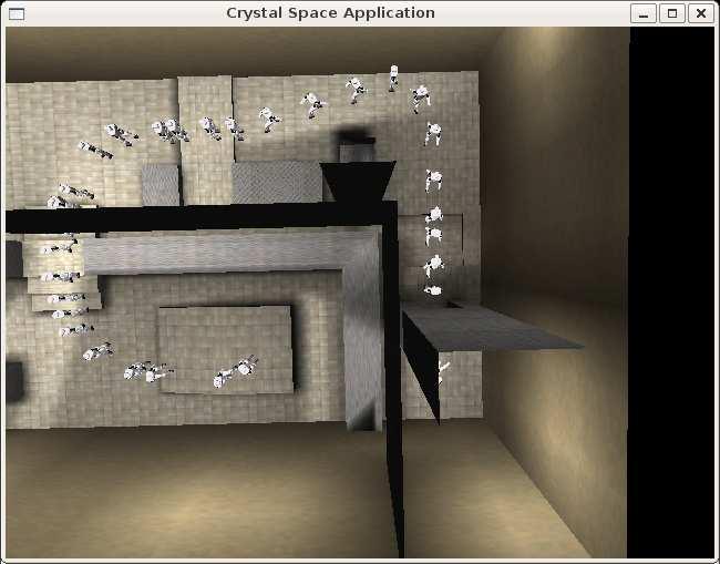
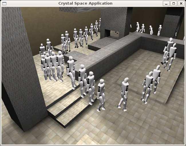
79 Figure B.2: Path for workspace 1 72

80 B.2 Map 2, Course 1 Figure B.3 shows M plan on M d and M skel on M n for the simulation of plan 1 in workspace 2. Figure B.4 shows the motion of the robot for this simulation at various angles. (a) M plan on M d (b) M skel on M n Figure B.3: Maps for workspace 2, course 1 Figure B.4: Path for workspace 2, course 1 73

81 B.3 Map 2, Course 2 Figure B.5 shows M plan on M d and M skel on M n for the simulation of plan 2 in workspace 2. Figure B.6 shows the motion of the robot for this simulation at various angles. (a) M plan on M d (b) M skel on M n Figure B.5: Maps for workspace 2, course 2 Figure B.6: Path for workspace 2, course 2 74

82 B.4 Map 2, Course 3 Figure B.7 shows M plan on M d and M skel on M n for the simulation of plan 3 in workspace 2. Figure B.8 shows the motion of the robot for this simulation at various angles. (a) M plan on M d (b) M skel on M n Figure B.7: Maps for workspace 2, course 3 Figure B.8: Path for workspace 2, course 3 75

83 B.5 Map 2, Course 4 Figure B.9 shows M plan on M d and M skel on M n for the simulation of plan 4 in workspace 2. Figure B.10 shows the motion of the robot for this simulation at various angles. (a) M plan on M d (b) M skel on M n Figure B.9: Maps for workspace 2, course 4 Figure B.10: Path for workspace 2, course 4 76

84 B.6 Map 3 Figure B.11 shows M plan on M d and M skel on M n for the simulation in workspace 3. Figure B.12 shows the motion of the robot for this simulation at various angles. (a) M plan on M d (b) M skel on M n Figure B.11: Maps for workspace 3 Figure B.12: Path for workspace 3 77